Investigating the nature of light scalar mesons with semileptonic decays of $\bm{D}$ mesons

Abstract

We study the semileptonic decays of $D_{s}^{+}$, $D^{+}$, and $D^{0}$ mesons into the light scalar mesons [$f_{0}(500)$, $K_{0}^{\ast}(800)$, $f_{0}(980)$, and $a_{0}(980)$] and the light vector mesons [$\rho(770)$, $\omega(782)$, $K^{\ast}(892)$, and $\phi(1020)$]. With the help of a chiral unitarity approach in coupled channels, we compute the branching fractions for scalar meson processes of the semileptonic $D$ decays in a simple way. Using current known values of the branching fractions, we make predictions for the branching fractions of the semileptonic decay modes with other scalar and vector mesons. Furthermore, we calculate the $\pi^{+}\pi^{-}$, $\pi\eta$, $\pi K$, and $K^{+}K^{-}$ invariant mass distributions in the semileptonic decays of $D$ mesons, which will help us clarify the nature of the light scalar mesons.

I Introduction

The recent experimental situation in hadron physics enables us to utilize huge amounts of data on heavy hadrons, which contain charm or bottom quark(s), for the investigation of hadron structures. Especially, decay properties of heavy mesons can shed more light on the nature of the light scalar mesons [$f_{0}(500)$, $K_{0}^{\ast}(800)$, $f_{0}(980)$, and $a_{0}(980)$], which has been a hot topic in hadron physics Agashe:2014kda . For instance, the decay $B_{s}^{0}\to J/\psi\pi^{+}\pi^{-}$ has been experimentally measured in Refs. Aaij:2011fx ; Li:2011pg ; Aaltonen:2011nk ; Abazov:2011hv ; LHCb:2012ae for the study of the $f_{0}(500)$ and $f_{0}(980)$ resonances, and they observed a pronounced peak for the $f_{0}(980)$ while no evident signal was found for the $f_{0}(500)$. Then a theoretical study Liang:2014tia followed the experiments and reproduced ratios of experimental branching fractions at a quantitative level, pointing out that $J/\psi+(s\bar{s})$ production in the $B_{s}^{0}$ decay and a hadronization of $s\bar{s}$ to $K\bar{K}$ are essential to understand the branching fractions of the $B_{s}^{0}$ decay into $J/\psi f_{0}(980)$. In the theoretical study, the final state interaction between two pseudoscalar mesons is calculated with the so-called chiral unitary approach Oller:1997ti ; Kaiser:1998fi ; Locher:1997gr ; Oller:1997ng ; Oller:1998hw ; Oller:1998zr ; Nieves:1999bx ; Pelaez:2006nj ; Albaladejo:2008qa , in which the light scalar mesons are obtained as dynamically generated resonances, and it is concluded that the $f_{0}(980)$ has a substantial fraction of the strange quarks. The same hadronization scheme has been employed in theoretical studies in Refs. MartinezTorres:2009uk ; Liang:2014tia ; Xie:2014tma ; Navarra:2015iea .

Figure 1: (a) Semileptonic decay of $D_{s}^{+}$ into $l^{+}\nu_{l}$ and a primary $s\bar{s}$ pair. (b) Semileptonic decay of $D_{s}^{+}$ into $l^{+}\nu_{l}$ and two pseudoscalar mesons $P$ with a hadronization.

In this paper, we consider the semileptonic decay of $D\to\text{hadron(s)}+l^{+}\nu_{l}$, extending a discussion for the semileptonic $B$ decays into $D_{s0}^{\ast}(2317)$ and $D_{0}^{\ast}(2400)$ resonances in Ref. Navarra:2015iea . The semileptonic $D$ decays have been experimentally investigated in, e.g., BES Ablikim:2006ah ; Ablikim:2006hw , FOCUS Link:2004gp ; Link:2005xe , BaBar Aubert:2008rs ; delAmoSanchez:2010fd , and CLEO Yelton:2009aa ; Ecklund:2009aa ; Martin:2011rd ; Yelton:2010js ; CLEO:2011ab . Here, in order to grasp how the semileptonic decay takes place, let us consider the $D_{s}^{+}$ meson. Since the constituent quark component of $D_{s}^{+}$ is $c\bar{s}$, we expect a Cabibbo favored semileptonic decay of $c\to s\,l^{+}\,\nu_{l}$ and hence the decay $D_{s}^{+}\to(s\bar{s})\,l^{+}\,\nu_{l}$ with $s\bar{s}$ being the vector meson $\phi(1020)$, which is depicted in Fig. 1(a). Actually this semileptonic decay mode has been observed in experiments, and its branching fraction to the total decay width is $\mathcal{B}[D_{s}^{+}\to\phi(1020)\,e^{+}\,\nu_{e}]=2.49\pm 0.14\%$ Agashe:2014kda (see Table 1, in which we list branching fractions for the semileptonic decays of $D_{s}^{+}$, $D^{+}$, and $D^{0}$ reported by the Particle Data Group). On the other hand, we cannot straightforwardly extend the discussion to the scalar meson productions in the final state of the semileptonic decays, since the structure of the scalar mesons, whether $q\bar{q}$ or some exotic one, is still controversial. In this study we consider the production of the $f_{0}(980)$ or $f_{0}(500)$ as dynamically generated resonances in the semileptonic $D_{s}^{+}$ decay, so we have to introduce an extra $\bar{q}q$ pair to make a hadronization as shown in Fig. 1(b). The introduction of an extra $\bar{q}q$ pair to make a hadronization has been performed in Refs. MartinezTorres:2009uk ; Liang:2014tia ; Xie:2014tma ; Navarra:2015iea . In this study we apply the same method of the hadronization to the semileptonic decays of $D$ mesons so as to investigate the nature of the light scalar mesons.

Table 1: Branching fractions for the semileptonic decays of $D_{s}^{+}$, $D^{+}$, and $D^{0}$ reported by the Particle Data Group Agashe:2014kda . In this Table we only show decay modes relevant to this study.

$D_{s}^{+}$
Mean life [s]	$(500\pm 7)\times 10^{-15}$
$\mathcal{B}[\phi(1020)e^{+}\nu_{e}]$	$(2.49\pm 0.14)\times 10^{-2}$
$\mathcal{B}[\omega(782)e^{+}\nu_{e}]$	$<2.0\times 10^{-3}$
$\mathcal{B}[K^{\ast}(892)^{0}e^{+}\nu_{e}]$	$(1.8\pm 0.7)\times 10^{-3}$
$\mathcal{B}[f_{0}(980)e^{+}\nu_{e},\,f_{0}(980)\to\pi^{+}\pi^{-}]$	$(2.00\pm 0.32)\times 10^{-3}$
$D^{+}$
Mean life [s]	$(1040\pm 7)\times 10^{-15}$
$\mathcal{B}[\bar{K}^{\ast}(892)^{0}e^{+}\nu_{e},\,\bar{K}^{\ast}(892)^{0}\to K^{-}\pi^{+}]$	$(3.68\pm 0.10)\times 10^{-2}$
$\mathcal{B}[(K^{-}\pi^{+})_{s\text{-wave}}e^{+}\nu_{e}]$	$(2.32\pm 0.10)\times 10^{-3}$
$\mathcal{B}[\bar{K}^{\ast}(892)^{0}\mu^{+}\nu_{\mu},\,\bar{K}^{\ast}(892)^{0}\to K^{-}\pi^{+}]$	$(3.52\pm 0.10)\times 10^{-2}$
$\mathcal{B}[\rho(770)^{0}e^{+}\nu_{e}]$	$(2.18^{+0.17}_{-0.25})\times 10^{-3}$
$\mathcal{B}[\rho(770)^{0}\mu^{+}\nu_{\mu}]$	$(2.4\pm 0.4)\times 10^{-3}$
$\mathcal{B}[\omega(782)e^{+}\nu_{e}]$	$(1.82\pm 0.19)\times 10^{-3}$
$\mathcal{B}[\phi(1020)e^{+}\nu_{e}]$	$<9\times 10^{-5}$
$D^{0}$
Mean life [s]	$(410.1\pm 1.5)\times 10^{-15}$
$\mathcal{B}[K^{\ast}(892)^{-}e^{+}\nu_{e}]$	$(2.16\pm 0.16)\times 10^{-2}$
$\mathcal{B}[K^{\ast}(892)^{-}\mu^{+}\nu_{\mu}]$	$(1.90\pm 0.24)\times 10^{-2}$
$\mathcal{B}[K^{-}\pi^{0}e^{+}\nu_{e}]$	$(1.6^{+1.3}_{-0.5})\times 10^{-2}$
$\mathcal{B}[\bar{K}^{0}\pi^{-}e^{+}\nu_{e}]$	$(2.7^{+0.9}_{-0.7})\times 10^{-2}$
$\mathcal{B}[\rho(770)^{-}e^{+}\nu_{e}]$	$(1.9\pm 0.4)\times 10^{-3}$

Utilizing the semileptonic decay of a heavy hadron provides us with two advantages when we investigate the internal structure of hadrons in the final state of the semileptonic decay. First, Cabibbo favored and suppressed processes enable us to specify flavors of quarks contained in final state hadrons. Second, the semileptonic decay of the heavy hadron to two light hadrons $+l^{+}\nu_{l}$ brings a suitable condition to measure effects of the final state interaction of the two light hadrons, since the leptons and hadrons in the final state interact with each other only weakly.

Theoretical work on the issues of the semileptonic $D$ decays is already available. In Ref. Bediaga:2003zh , using QCD sum rules, the $D_{s}^{+}$ and $D^{+}$ semileptonic decays into $f_{0}(980)$ are considered concluding that the importance of up and down quarks in the $f_{0}(980)$ is not negligible. In Ref. Ke:2009ed the $D_{s}^{+}\to f_{0}(980)e^{+}\nu_{e}$ reaction is analyzed from the point of view of the $f_{0}(980)$ being a $q\bar{q}$ state, concluding that $s\bar{s}$ component of the $f_{0}(980)$ may not be dominant. In Ref. Achasov:2012kk the $D_{s}^{+}\to\pi^{+}\pi^{-}e^{+}\nu_{e}$ reaction is studied concluding that it supports the dominant four quark nature of the $f_{0}(500)$ and $f_{0}(980)$. Similar conclusions about the four quark nature of the scalar mesons are reached in the work of Fariborz:2011xb ; Fariborz:2014mpa . Research along the same line is done in Ref. Wang:2009azc , looking for likely reasonable ratios that would help distinguish between the two and four quark structure of the scalar mesons.

Another line of research is done using light-cone sum rules to evaluate the form factors appearing in the process Meissner:2013hya . This line of research is applied in many related processes, rare decays like $B_{s}\to\pi^{+}\pi^{-}l^{+}l^{-}$ in Wang:2015paa , $B_{s}\to K^{(\ast)}l\bar{\nu}$ in Meissner:2013pba , $B^{0}_{(s)}\to J/\psi\pi^{+}\pi^{-}$ and $B_{s}\to\pi^{+}\pi^{-}\mu^{+}\mu^{-}$ decays in Wang:2015uea , or semileptonic decays Kang:2013jaa ; Doring:2013wka ; Shi:2015kha . In some cases the meson final state interaction is further implemented using the Omnes representation Meissner:2013hya ; Doring:2013wka , while in other cases Breit–Wigner or Flatte structures are implemented and parametrized to account for the resonances observed in the experiment.

In contrast to these pictures, in the present study we treat the scalar mesons as dynamically generated resonances from two pseudoscalar mesons in the so-called chiral unitary approach. Then we describe the semileptonic decays of $D$ mesons in an economical way for hadronization as done in Refs. MartinezTorres:2009uk ; Liang:2014tia ; Xie:2014tma ; Navarra:2015iea .

This paper is organized as follows. In Sec. II we formulate the semileptonic decay widths of $D_{s}^{+}$, $D^{+}$, and $D^{0}$ into the light scalar and vector mesons and give our model of the hadronization. We also calculate meson–meson scattering amplitudes to generate dynamically the scalar mesons. In Sec. III we show our numerical results of the semileptonic decay widths of $D_{s}^{+}$, $D^{+}$, and $D^{0}$. We predict branching fractions which are not reported by the Particle Data Group and show invariant mass distributions of the two pseudoscalar mesons from the scalar and vector mesons. Section IV is devoted to drawing the conclusion of this study.

II Formulation

Table 2: Semileptonic decay modes of $D_{s}^{+}$, $D^{+}$, and $D^{0}$ considered in this study. The lepton flavor $l$ is $e$ and $\mu$. We also specify Cabibbo favored/suppressed process for each decay mode; the semileptonic decay into two pseudoscalar mesons is judged with the discussions given in Sec. II.2.

$D_{s}^{+}$
$\phi(1020)\,l^{+}\,\nu_{l}$	favored
$K^{\ast}(892)^{0}\,l^{+}\,\nu_{l}$	suppressed
$\pi^{+}\pi^{-}\,l^{+}\,\nu_{l}$	favored
$K^{+}K^{-}\,l^{+}\,\nu_{l}$	favored
$\pi^{-}K^{+}\,l^{+}\,\nu_{l}$	suppressed
$D^{+}$
$\bar{K}^{\ast}(892)^{0}\,l^{+}\,\nu_{l}$	favored
$\rho(770)^{0}\,l^{+}\,\nu_{l}$	suppressed
$\omega(782)\,l^{+}\,\nu_{l}$	suppressed
$\pi^{+}\pi^{-}\,l^{+}\,\nu_{l}$	suppressed
$\pi^{0}\eta\,l^{+}\,\nu_{l}$	suppressed
$K^{+}K^{-}\,l^{+}\,\nu_{l}$	suppressed
$\pi^{+}K^{-}\,l^{+}\,\nu_{l}$	favored
$D^{0}$
$K^{\ast}(892)^{-}\,l^{+}\,\nu_{l}$	favored
$\rho(770)^{-}\,l^{+}\,\nu_{l}$	suppressed
$\pi^{-}\eta\,l^{+}\,\nu_{l}$	suppressed
$K^{0}K^{-}\,l^{+}\,\nu_{l}$	suppressed
$\pi^{-}\bar{K}^{0}\,l^{+}\,\nu_{l}$	favored

In this section we formulate the semileptonic decay widths of $D_{s}^{+}$, $D^{+}$, and $D^{0}$ into light scalar and vector mesons:

$$D_{s}^{+},\,D^{+},\,D^{0}\to\begin{cases}Sl^{+}\nu_{l},\quad S\to PP,\\ Vl^{+}\nu_{l},\end{cases}$$ (1)

where $S$, $V$, and $P$ represent the light scalar, vector, and pseudoscalar mesons, respectively, and the lepton flavor $l$ can be $e$ and $\mu$. Explicit decay modes are listed in Table 2. In order to formulate the decay width, we consider first the semileptonic decay amplitudes and widths in Section II.1 and next hadronizations into scalar and vector mesons in Section II.2. Scattering amplitudes of two pseudoscalar mesons are then constructed in the chiral unitary approach for the description of the scalar mesons in Section II.3. Throughout this study we assume isospin symmetry for light hadrons.

II.1 Amplitudes and widths of semileptonic $\bm{D}$ decays

In general, we can express the decay amplitude of $D\to\text{hadron(s)}+l^{+}\nu_{l}$, $T_{D}$, by using the propagator of the $W$ boson and its couplings to leptons and quarks, which can be replaced with the Fermi coupling constant $G_{\rm F}$. At this stage we do not fix the number of the final state hadrons. In a similar manner to the formulation in Ref. Navarra:2015iea , the explicit form of $T_{D}$ becomes

$$T_{D}=-i\frac{G_{\rm F}}{\sqrt{2}}L^{\alpha}Q_{\alpha}\times V_{\rm had}.$$ (2)

The factor $V_{\rm had}$ consists of the wave function of quarks inside the $D$ meson, the hadronization contribution in the final state, and the Cabibbo–Kobayashi–Maskawa matrix element for the transition from the charm to a light quark. The explicit form of $V_{\rm had}$ will be determined in the next subsection. The lepton and quark parts of the $W$ boson couplings are defined as.

$$L^{\alpha}\equiv\overline{u}_{\nu}\gamma^{\alpha}(1-\gamma_{5})v_{l},\quad Q_{\alpha}\equiv\overline{u}_{q}\gamma_{\alpha}(1-\gamma_{5})u_{c},$$ (3)

respectively, where $u_{\nu}$, $v_{l}$, $u_{q}$, and $u_{c}$ are the Dirac spinors corresponding to the neutrino, lepton $l^{+}$, light quark $q$, and charm quark, respectively.

Let us now calculate the squared amplitude for the semileptonic $D$ decay widths, in which we average (sum) the polarizations of the initial-state quarks (final state leptons and quarks). Therefore, in terms of the amplitude in Eq. (2), we can obtain the squared decay amplitude as

$$\frac{1}{2}\sum_{\rm pol}|T_{D}|^{2}=\frac{|G_{\rm F}V_{\rm had}|^{2}}{4}\sum_{\rm pol}|L^{\alpha}Q_{\alpha}|^{2}$$ (4)

where the factor $1/2$ comes from the average of the charm quark polarization in the initial state. We can further calculate the lepton and quark parts in the amplitude (3), by using the conventions of the Dirac spinors and traces of Dirac $\gamma$ matrices summarized in Appendix A, which lead to

$$\sum_{\rm pol}L^{\alpha}L^{\dagger\beta}= \text{tr}\left[\gamma^{\alpha}(1-\gamma_{5})\frac{\ooalign{\hfil/\hfil\crcr$p$}_{l}-m_{l}}{2m_{l}}(1+\gamma_{5})\gamma^{\beta}\frac{\ooalign{\hfil/\hfil\crcr$p$}_{\nu}+m_{\nu}}{2m_{\nu}}\right]$$ (9)

$$= 2\frac{p_{l}^{\alpha}p_{\nu}^{\beta}+p_{\nu}^{\alpha}p_{l}^{\beta}-p_{l}\cdot p_{\nu}g^{\alpha\beta}+i\epsilon^{\alpha\beta\rho\sigma}p_{l\rho}p_{\nu\sigma}}{m_{l}m_{\nu}},$$ (10)

where $p_{l}$ and $p_{\nu}$ ($m_{l}$ and $m_{\nu}$) are momenta (masses) of the lepton $l^{+}$ and neutrino, respectively, and

$$\sum_{\rm pol}Q_{\alpha}Q_{\beta}^{\dagger}= \text{tr}\left[\gamma_{\alpha}(1-\gamma_{5})\frac{\ooalign{\hfil/\hfil\crcr$p$}_{c}+m_{c}}{2m_{c}}(1+\gamma_{5})\gamma_{\beta}\frac{\ooalign{\hfil/\hfil\crcr$p$}_{q}+m_{q}}{2m_{q}}\right]$$ (15)

$$= 2\frac{p_{c\alpha}p_{q\beta}+p_{q\alpha}p_{c\beta}-p_{c}\cdot p_{q}g_{\alpha\beta}+i\epsilon_{\alpha\beta\rho\sigma}p_{c}^{\rho}p_{q}^{\sigma}}{m_{c}m_{q}},$$ (16)

with the momenta (masses) of the charm and light quarks, $p_{c}$ and $p_{q}$ ($m_{c}$ and $m_{q}$), respectively. Then with a straightforward calculation we have

$$\sum_{\rm pol}|L^{\alpha}Q_{\alpha}|^{2}=\frac{16(p_{l}\cdot p_{c})(p_{\nu}\cdot p_{q})}{m_{l}m_{\nu}m_{c}m_{q}}.$$ (17)

Now let us rewrite the momenta of quarks by using those of hadrons in the following manner:

$$\frac{p_{c}^{\mu}}{m_{c}}=\frac{p_{D}^{\mu}}{m_{D}},\quad\frac{p_{q}^{\mu}}{m_{q}}=\frac{p_{R}^{\mu}}{m_{R}},$$ (18)

where we have neglected the relative internal momenta of the quarks, which are typically small compared to the masses of quarks. Here $m_{D}$ and $m_{R}$ ($p_{D}$ and $p_{R}$) are the masses (momenta) of the $D$ and $R=S$, $V$ mesons, respectively. With these translations the square of $L^{\alpha}Q_{\alpha}$ with polarization summation becomes

$$\sum_{\rm pol}|L^{\alpha}Q_{\alpha}|^{2}=\frac{16(p_{l}\cdot p_{D})(p_{\nu}\cdot p_{R})}{m_{l}m_{\nu}m_{D}m_{R}}.$$ (19)

Therefore, we obtain the squared decay amplitude as:

$$\frac{1}{2}\sum_{\rm pol}|T_{D}|^{2}=\frac{4|G_{\rm F}V_{\rm had}|^{2}}{m_{l}m_{\nu}m_{D}m_{R}}(p_{l}\cdot p_{D})(p_{\nu}\cdot p_{R}).$$ (20)

With the above squared amplitude we can compute the decay width. We will be interested in two types of decays: three-body decays for vector mesons such as $D_{s}^{+}\to\phi(1020)\,e^{+}\,\nu_{e}$, and four-body decays for scalar mesons constructed from two pseudoscalar mesons such as $D_{s}^{+}\to\pi^{+}\pi^{-}\,e^{+}\,\nu_{e}$. As it will be seen, both decay types can be described by the amplitude $T_{D}$ with different assumptions for $V_{\rm had}$: $V_{\rm had}^{(v)}$ and $V_{\rm had}^{(s)}$ respectively.

The formula for the three-body decay is given by Agashe:2014kda :

$$\Gamma_{3}=\frac{m_{l}m_{\nu}}{128\pi^{5}m_{D}^{2}}\int dM_{\rm inv}^{(l\nu)}P_{\rm cm}\tilde{p}_{\nu}\int d\Omega\int d\tilde{\Omega}_{\nu}\frac{1}{2}\sum_{\rm pol}|T_{D}|^{2},$$ (21)

where $P_{\rm cm}$ is the momentum of the final state vector meson in the $D$ rest frame and $\tilde{p}_{\nu}$ is the momentum of the neutrino in the $l\nu$ rest frame, both of which are evaluated as

$$P_{\rm cm}=\frac{\lambda^{1/2}(m_{D}^{2},\,[M_{\rm inv}^{(l\nu)}]^{2},\,m_{V}^{2})}{2m_{D}},$$ (22)

$$\tilde{p}_{\nu}=\frac{\lambda^{1/2}([M_{\rm inv}^{(l\nu)}]^{2},\,m_{l}^{2},\,m_{\nu}^{2})}{2M_{\rm inv}^{(l\nu)}},$$ (23)

with the Källen function $\lambda(x,\,y,\,z)=x^{2}+y^{2}+z^{2}-2xy-2yz-2zx$ and the vector meson mass $m_{V}$. The tilde on characters for leptons indicates that they are evaluated in the $l\nu$ rest frame. The solid angles $\Omega$ and $\tilde{\Omega}_{\nu}$ are for the vector meson in the $D$ rest frame and for the neutrino in the $l\nu$ rest frame, respectively, and $M_{\rm inv}^{(l\nu)}$ is the $l\nu$ invariant mass. The integral range of $M_{\rm inv}^{(l\nu)}$ is $[m_{l}+m_{\nu},\,m_{D}-m_{V}]$. Substituting the squared amplitude with that in Eq. (20), we obtain

$$\Gamma_{3}= \frac{|G_{\rm F}|^{2}}{32\pi^{5}m_{D}^{3}m_{V}}\int dM_{\rm inv}^{(l\nu)}P_{\rm cm}\tilde{p}_{\nu}\int d\Omega\int d\tilde{\Omega}_{\nu}$$

$$\times\left|V_{\rm had}^{(v)}\right|^{2}(p_{l}\cdot p_{D})(p_{\nu}\cdot p_{V}).$$ (24)

In general, the hadronization part $V_{\rm had}$ may depend on the energy and scattering angles, and hence one cannot put it out of the integral. In this study, however, $V_{\rm had}^{(v)}$ will be simply constructed, so that this will not depend on $M_{\rm inv}^{(l\nu)}$ nor the angle, as we will see in the next subsection. Furthermore, the integral of the solid angle $\tilde{\Omega}_{\nu}$ is performed in the $l\nu$ rest frame as Navarra:2015iea

$$\int d\tilde{\Omega}_{\nu}(p_{l}\cdot p_{D})(p_{\nu}\cdot p_{V})$$

$$=\int d\tilde{\Omega}_{\nu}(\tilde{E}_{l}\tilde{E}_{D}+\tilde{\bm{p}}_{\nu}\cdot\tilde{\bm{p}}_{D})(\tilde{E}_{\nu}\tilde{E}_{V}-\tilde{\bm{p}}_{\nu}\cdot\tilde{\bm{p}}_{D})$$

$$=4\pi\tilde{E}_{l}\tilde{E}_{\nu}\tilde{E}_{D}\tilde{E}_{V}-\frac{4\pi}{3}|\tilde{\bm{p}}_{\nu}|^{2}|\tilde{\bm{p}}_{D}|^{2}$$

$$=\pi[M_{\rm inv}^{(l\nu)}]^{2}\left(\tilde{E}_{D}\tilde{E}_{V}-\frac{1}{3}|\tilde{\bm{p}}_{D}|^{2}\right),$$ (25)

where $\tilde{E}$ and $\tilde{\bm{p}}$ are the energies and momenta in the $l\nu$ rest frame. At the first equality we have used relations $\tilde{\bm{p}}_{l}=-\tilde{\bm{p}}_{\nu}$ and $\tilde{\bm{p}}_{V}=\tilde{\bm{p}}_{D}$, while at the third equality we have used relations obtained by neglecting masses of leptons:

$$\tilde{E}_{l}=\tilde{E}_{\nu}=|\tilde{\bm{p}}_{\nu}|=\frac{M_{\rm inv}^{(l\nu)}}{2}.$$ (26)

The energies and momentum of hadrons in the $l\nu$ rest frame can be exactly evaluated as

$$\tilde{E}_{D}=\frac{m_{D}^{2}+[M_{\rm inv}^{(l\nu)}]^{2}-m_{V}^{2}}{2M_{\rm inv}^{(l\nu)}},$$ (27)

$$\tilde{E}_{V}=\frac{m_{D}^{2}-[M_{\rm inv}^{(l\nu)}]^{2}-m_{V}^{2}}{2M_{\rm inv}^{(l\nu)}},$$ (28)

and $|\tilde{\bm{p}}_{D}|^{2}=\tilde{E}_{D}^{2}-m_{D}^{2}$. As a consequence, we have

$$\Gamma_{3}=\frac{\left|G_{\rm F}V_{\rm had}^{(v)}\right|^{2}}{8\pi^{3}m_{D}^{3}m_{V}} \int dM_{\rm inv}^{(l\nu)}P_{\rm cm}\tilde{p}_{\nu}[M_{\rm inv}^{(l\nu)}]^{2}$$

$$\times\left(\tilde{E}_{D}\tilde{E}_{V}-\frac{1}{3}|\tilde{\bm{p}}_{D}|^{2}\right),$$ (29)

where we have performed the integral of the solid angle $\Omega$.

In a similar way, we can evaluate the decay width for the four-body final state. The formula for the four-body decay is given by

$$\Gamma_{4}= \frac{m_{l}m_{\nu}}{2048\pi^{8}m_{D}^{2}}\int dM_{\rm inv}^{(hh)}\int dM_{\rm inv}^{(l\nu)}P_{\rm cm}^{\prime}\tilde{p}_{h}\tilde{p}_{\nu}$$

$$\times\int d\Omega^{\prime}\int d\tilde{\Omega}_{h}\int d\tilde{\Omega}_{\nu}\frac{1}{2}\sum_{\rm pol}|T_{D}|^{2},$$ (30)

where $M_{\rm inv}^{(hh)}$ is the invariant mass of the two-meson system ($hh$), $P_{\rm cm}^{\prime}$ is the center-of-mass momentum of the two-meson system in the $D$ rest frame and $\tilde{p}_{h}$ is the momentum of a meson in the $hh$ rest frame, both of which are evaluated as

$$P_{\rm cm}^{\prime}=\frac{\lambda^{1/2}(m_{D}^{2},\,[M_{\rm inv}^{(hh)}]^{2},\,[M_{\rm inv}^{(l\nu)}]^{2})}{2m_{D}},$$ (31)

$$\tilde{p}_{h}=\frac{\lambda^{1/2}([M_{\rm inv}^{(hh)}]^{2},\,m_{h}^{2},\,m_{h}^{\prime 2})}{2M_{\rm inv}^{(hh)}},$$ (32)

with the meson masses $m_{h}$ and $m_{h}^{\prime}$. The momentum of the neutrino in the $l\nu$ rest frame $\tilde{p}_{\nu}$ is given in Eq. (23). The solid angles $\Omega^{\prime}$ and $\tilde{\Omega}_{h}$ are for the two-meson system in the $D$ rest frame and for a meson in the $hh$ rest frame, respectively. The tilde on characters for mesons indicates that they are evaluated in the $hh$ rest frame. Since we are interested in the meson–meson invariant mass distributions for the semileptonic $D$ decay, we calculate the differential decay width $d\Gamma_{4}/dM_{\rm inv}^{(hh)}$. Then in a similar manner to the case of the three-body decay, we have

$$\frac{d\Gamma_{4}}{dM_{\rm inv}^{(hh)}}=\frac{\left|G_{\rm F}V_{\rm had}^{(s)}\right|^{2}}{32\pi^{5}m_{D}^{3}M_{\rm inv}^{(hh)}} \int dM_{\rm inv}^{(l\nu)}P_{\rm cm}^{\prime}\tilde{p}_{h}\tilde{p}_{\nu}[M_{\rm inv}^{(l\nu)}]^{2}$$

$$\times\left(\tilde{E}_{D}\tilde{E}_{S}-\frac{1}{3}|\tilde{\bm{p}}_{D}|^{2}\right),$$ (33)

where we have performed the integrals with respect to the solid angles $\Omega^{\prime}$ and $\tilde{\Omega}_{h}$. We mention that $V_{\rm had}^{(s)}$ will be simply constructed as well, so that this can be put out of the integral, as we will see in the next subsection. The two-meson invariant mass $M_{\rm inv}^{(hh)}$ can take a value within $[m_{h}+m_{h}^{\prime},\,m_{D}-m_{l}-m_{\nu}]$, while the integral range of $M_{\rm inv}^{(l\nu)}$ is $[m_{l}+m_{\nu},\,m_{D}-M_{\rm inv}^{(hh)}]$. The energies and momentum of hadrons in the parentheses can be exactly evaluated as

$$\tilde{E}_{D}=\frac{m_{D}^{2}+[M_{\rm inv}^{(l\nu)}]^{2}-[M_{\rm inv}^{(hh)}]^{2}}{2M_{\rm inv}^{(l\nu)}},$$ (34)

$$\tilde{E}_{S}=\frac{m_{D}^{2}-[M_{\rm inv}^{(l\nu)}]^{2}-[M_{\rm inv}^{(hh)}]^{2}}{2M_{\rm inv}^{(l\nu)}},$$ (35)

and $|\tilde{\bm{p}}_{D}|^{2}=\tilde{E}_{D}^{2}-m_{D}^{2}$.

II.2 Hadronizations

Figure 2: Diagrammatic representation of the direct plus rescattering processes for two pseudoscalar mesons. The solid and dashed lines denote quarks and pseudoscalar mesons, respectively. The shaded ellipses indicate the hadronization of a quark–antiquark pair into two pseudoscalar mesons, while the open circle indicates the rescattering of two pseudoscalar mesons.

Next we fix the mechanism for the appearance of the scalar and vector mesons in the final state of the semileptonic decay. We here note that, for the scalar and vector mesons in the final state, the hadronization processes should be different from each other according to their structure. For the scalar mesons, we employ the chiral unitary approach Oller:1997ti ; Kaiser:1998fi ; Locher:1997gr ; Oller:1997ng ; Oller:1998hw ; Oller:1998zr ; Nieves:1999bx ; Pelaez:2006nj ; Albaladejo:2008qa , in which the scalar mesons are dynamically generated from the interaction of two pseudoscalar mesons governed by the chiral Lagrangians. Therefore, in this picture the light quark–antiquark pair after the $W$ boson emission gets hadronized by adding an extra $\bar{q}q$ with the quantum number of the vacuum, $\bar{u}u+\bar{d}d+\bar{s}s$, which results in two pseudoscalar mesons in the final state [see Fig. 1(b)]. Then the scalar mesons are obtained as a consequence of the final state interaction of the two pseudoscalar mesons as diagrammatically shown in Fig. 2. For the vector mesons, on the other hand, hadronization with an extra $\bar{q}q$ is unnecessary since they are expected to consist genuinely of a light quark–antiquark pair [see Fig. 1(a)].

II.2.1 Scalar mesons

First we consider processes with the scalar mesons in the final state as the dynamically generated resonances. The basic idea of the hadronization with an extra $\bar{q}q$ with the quantum number of the vacuum has already shown in Refs. MartinezTorres:2009uk ; Liang:2014tia ; Xie:2014tma ; Navarra:2015iea . We start with the $q\bar{q}$ matrix $M$:

$$M=\left(\begin{array}[]{ccc}u\bar{u}&u\bar{d}&u\bar{s}\\ d\bar{u}&d\bar{d}&d\bar{s}\\ s\bar{u}&s\bar{d}&s\bar{s}\\ \end{array}\right).$$ (36)

One can easily check that this matrix has the property

$$M\cdot M=M(\bar{u}u+\bar{d}d+\bar{s}s).$$ (37)

With this property, a $q_{f}\bar{q}_{f^{\prime}}$ pair after the $W$ boson emission can be added by an extra $\bar{q}q$ to be

$$q_{f}\bar{q}_{f^{\prime}}\to(M\cdot M)_{ff^{\prime}},$$ (38)

where $f$ denotes the flavor of light quarks: $q_{1}=u$, $q_{2}=d$, and $q_{3}=s$. Next we rewrite the matrix $M$ in terms of the matrix $\phi$ for pseudoscalar mesons

$$\phi=\left(\begin{array}[]{ccc}\frac{1}{\sqrt{2}}\pi^{0}+\frac{1}{\sqrt{3}}\eta+\frac{1}{\sqrt{6}}\eta^{\prime}&\pi^{+}&K^{+}\\ \pi^{-}&-\frac{1}{\sqrt{2}}\pi^{0}+\frac{1}{\sqrt{3}}\eta+\frac{1}{\sqrt{6}}\eta^{\prime}&K^{0}\\ K^{-}&\bar{K}^{0}&-\frac{1}{\sqrt{3}}\eta+\sqrt{\frac{2}{3}}\eta^{\prime}\\ \end{array}\right),$$ (39)

where we have taken into account the $\eta$–$\eta^{\prime}$ mixing in a standard way Bramon:1992kr . In this scheme we can calculate the weight of each pair of pseudoscalar mesons in the hadronization. Namely, the $s\bar{s}$ pair gets hadronized as $s\bar{s}(\bar{u}u+\bar{d}d+\bar{s}s)\equiv(\phi\cdot\phi)_{33}$, where

$$(\phi\cdot\phi)_{33} =K^{-}K^{+}+\bar{K}^{0}K^{0}+\frac{1}{3}\eta\eta.$$ (40)

Here and in the following we omit the $\eta^{\prime}$ contribution since $\eta^{\prime}$ is irrelevant to the description of the scalar mesons due to its large mass. In similar manners, the $d\bar{s}$, $s\bar{d}$, $d\bar{d}$, $s\bar{u}$, and $d\bar{u}$ pairs get hadronized as

$$(\phi\cdot\phi)_{23}=\pi^{-}K^{+}-\frac{1}{\sqrt{2}}\pi^{0}K^{0},$$ (41)

$$(\phi\cdot\phi)_{32}= K^{-}\pi^{+}-\frac{1}{\sqrt{2}}\bar{K}^{0}\pi^{0},$$ (42)

$$(\phi\cdot\phi)_{22} =\pi^{-}\pi^{+}+\frac{1}{2}\pi^{0}\pi^{0}+\frac{1}{3}\eta\eta-\sqrt{\frac{2}{3}}\pi^{0}\eta+K^{0}\bar{K}^{0},$$ (43)

$$(\phi\cdot\phi)_{31}=\frac{1}{\sqrt{2}}\pi^{0}K^{-}+\pi^{-}\bar{K}^{0},$$ (44)

and

$$(\phi\cdot\phi)_{21}=\frac{2}{\sqrt{3}}\pi^{-}\eta+K^{0}K^{-},$$ (45)

respectively.

By using these weights, we can express the hadronization amplitude for the scalar mesons, $V_{\rm had}^{(s)}$, in terms of two pseudoscalar mesons. For instance, we want to reconstruct $f_{0}(500)$ and $f_{0}(980)$ from the $\pi^{+}\pi^{-}$ system in the $D_{s}^{+}\to\pi^{+}\pi^{-}\,l^{+}\,\nu_{l}$ decay. Because of the quark configuration in the parent particle $D_{s}^{+}$, in this decay the $\pi^{+}\pi^{-}$ system should be obtained from the hadronization of the $s\bar{s}$ pair and the rescattering process for two pseudoscalar mesons, as seen in Fig. 2, with the weight in Eq. (40). Therefore, for the $D_{s}^{+}\to\pi^{+}\pi^{-}\,l^{+}\,\nu_{l}$ decay mode we can express the hadronization amplitude with a prefactor $C$ and the Cabibbo–Kobayashi–Maskawa matrix elements $V_{cs}$ as

$$V_{\rm had}^{(s)}[D_{s}^{+},\,\pi^{+}\pi^{-}]=CV_{cs}\left(G_{K^{+}K^{-}}T_{K^{+}K^{-}\to\pi^{+}\pi^{-}}\phantom{\frac{1}{2}}\right.$$

$$\left.+G_{K^{0}\bar{K}^{0}}T_{K^{0}\bar{K}^{0}\to\pi^{+}\pi^{-}}+\frac{1}{3}\cdot 2\cdot\frac{1}{2}G_{\eta\eta}T_{\eta\eta\to\pi^{+}\pi^{-}}\right).$$ (46)

In this equation, the decay mode is abbreviated as $[D_{s}^{+},\,\pi^{+}\pi^{-}]$, and $G$ and $T$ are the loop function and scattering amplitude of two pseudoscalar mesons, respectively, whose formulation are given in Sec. II.3. We have introduced extra factors $2$ and $1/2$ for the identical particles $\eta\eta$. The former factor $2$ comes from the two ways of annihilating the $\eta\eta$ operator in Eq. (40) by the $|\eta\eta\rangle$ state as in the usual manner for effective Lagrangians, while the latter one $1/2$ is the symmetry factor for the $\eta\eta$ loop. The scalar mesons $f_{0}(500)$ and $f_{0}(980)$ appear in the rescattering process and exist in the scattering amplitude $T$ for two pseudoscalar mesons. It is important that this is a Cabibbo favored process with $V_{cs}$. Furthermore, since the $s\bar{s}$ pair is hadronized, this is sensitive to the component of the strange quark in the scalar mesons. In this study we assume that $C$ is a constant, and hence the hadronization amplitude $V_{\rm had}^{(s)}$ is a function only of the invariant mass of two pseudoscalar mesons. Here we emphasize that the prefactor $C$ should be common to all reactions for scalar meson productions, because in the hadronization the SU(3) flavor symmetry is reasonable, i.e., the light quark–antiquark pair $q_{f}\bar{q}_{f^{\prime}}$ hadronizes in the same way regardless of the quark flavor $f$. In this sense we obtain

$$V_{\rm had}^{(s)}[D_{s}^{+},\,K^{+}K^{-}]=CV_{cs}\left(1+G_{K^{+}K^{-}}T_{K^{+}K^{-}\to K^{+}K^{-}}\phantom{\frac{1}{2}}\right.$$

$$\left.+G_{K^{0}\bar{K}^{0}}T_{K^{0}\bar{K}^{0}\to K^{+}K^{-}}+\frac{1}{3}\cdot 2\cdot\frac{1}{2}G_{\eta\eta}T_{\eta\eta\to K^{+}K^{-}}\right),$$ (47)

for the $D_{s}^{+}\to K^{+}K^{-}\,l^{+}\,\nu_{l}$ decay. In this case we have to take into account the direct production of the two pseudoscalar mesons without rescattering (the first diagram in Fig. 2), which results in the unity in the parentheses. On the other hand, for the $D_{s}^{+}\to\pi^{-}K^{+}\,l^{+}\,\nu_{l}$ decay mode the $\pi^{-}K^{+}$ system should be obtained from the hadronization of $d\bar{s}$ and hence this is a Cabibbo suppressed decay mode. The hadronization amplitude is expressed as

$$V_{\rm had}^{(s)}[D_{s}^{+},\,\pi^{-}K^{+}]=CV_{cd}\left(1+G_{\pi^{-}K^{+}}T_{\pi^{-}K^{+}\to\pi^{-}K^{+}}\phantom{\frac{1}{\sqrt{2}}}\right.$$

$$\left.\quad\quad\quad\quad-\frac{1}{\sqrt{2}}G_{\pi^{0}K^{0}}T_{\pi^{0}K^{0}\to\pi^{-}K^{+}}\right).$$ (48)

In a similar manner we can construct every hadronization amplitude for the scalar meson. The resulting expressions are as follows:

$$V_{\rm had}^{(s)}[D^{+},\,\pi^{+}\pi^{-}]=CV_{cd}\left(1+G_{\pi^{+}\pi^{-}}T_{\pi^{+}\pi^{-}\to\pi^{+}\pi^{-}}\phantom{\frac{1}{2}}\right.$$

$$+\frac{1}{2}\cdot 2\cdot\frac{1}{2}G_{\pi^{0}\pi^{0}}T_{\pi^{0}\pi^{0}\to\pi^{+}\pi^{-}}+\frac{1}{3}\cdot 2\cdot\frac{1}{2}G_{\eta\eta}T_{\eta\eta\to\pi^{+}\pi^{-}}$$

$$\left.\!\!\!\!\!\!\phantom{\frac{1}{2}}+G_{K^{0}\bar{K}^{0}}T_{K^{0}\bar{K}^{0}\to\pi^{+}\pi^{-}}\right),$$ (49)

$$V_{\rm had}^{(s)}[D^{+},\,\pi^{0}\eta]=CV_{cd}\left(-\sqrt{\frac{2}{3}}-\sqrt{\frac{2}{3}}G_{\pi^{0}\eta}T_{\pi^{0}\eta\to\pi^{0}\eta}\right.$$

$$\left.\phantom{\sqrt{\frac{2}{3}}}\quad\quad\quad\quad+G_{K^{0}\bar{K}^{0}}T_{K^{0}\bar{K}^{0}\to\pi^{0}\eta}\right),$$ (50)

$$V_{\rm had}^{(s)}[D^{+},\,K^{+}K^{-}]=CV_{cd}\left(G_{\pi^{+}\pi^{-}}T_{\pi^{+}\pi^{-}\to K^{+}K^{-}}\phantom{\sqrt{\frac{1}{2}}}\right.$$

$$+\frac{1}{2}\cdot 2\cdot\frac{1}{2}G_{\pi^{0}\pi^{0}}T_{\pi^{0}\pi^{0}\to K^{+}K^{-}}+\frac{1}{3}\cdot 2\cdot\frac{1}{2}G_{\eta\eta}T_{\eta\eta\to K^{+}K^{-}}$$

$$\left.\!-\sqrt{\frac{2}{3}}G_{\pi^{0}\eta}T_{\pi^{0}\eta\to K^{+}K^{-}}+G_{K^{0}\bar{K}^{0}}T_{K^{0}\bar{K}^{0}\to K^{+}K^{-}}\right),$$ (51)

$$V_{\rm had}^{(s)}[D^{+},\,\pi^{+}K^{-}]=CV_{cs}\left(1+G_{\pi^{+}K^{-}}T_{\pi^{+}K^{-}\to\pi^{+}K^{-}}\phantom{\frac{1}{\sqrt{2}}}\right.$$

$$\left.\quad\quad\quad\quad-\frac{1}{\sqrt{2}}G_{\pi^{0}\bar{K}^{0}}T_{\pi^{0}\bar{K}^{0}\to\pi^{+}K^{-}}\right),$$ (52)

$$V_{\rm had}^{(s)}[D^{0},\,\pi^{-}\eta]=CV_{cd}\left(\frac{2}{\sqrt{3}}+\frac{2}{\sqrt{3}}G_{\pi^{-}\eta}T_{\pi^{-}\eta\to\pi^{-}\eta}\right.$$

$$\left.\phantom{\frac{2}{\sqrt{3}}}\quad\quad\quad\quad+G_{K^{0}K^{-}}T_{K^{0}K^{-}\to\pi^{-}\eta}\right),$$ (53)

$$V_{\rm had}^{(s)}[D^{0},\,K^{0}K^{-}]=CV_{cd}\left(1+\frac{2}{\sqrt{3}}G_{\pi^{-}\eta}T_{\pi^{-}\eta\to K^{0}K^{-}}\right.$$

$$\left.\phantom{\frac{2}{\sqrt{3}}}\quad\quad\quad\quad+G_{K^{0}K^{-}}T_{K^{0}K^{-}\to K^{0}K^{-}}\right),$$ (54)

$$V_{\rm had}^{(s)}[D^{0},\,\pi^{-}\bar{K}^{0}]=CV_{cs}\left(1+\frac{1}{\sqrt{2}}G_{\pi^{0}K^{-}}T_{\pi^{0}K^{-}\to\pi^{-}\bar{K}^{0}}\right.$$

$$\left.\phantom{\frac{1}{\sqrt{2}}}\quad\quad\quad\quad+G_{\pi^{-}\bar{K}^{0}}T_{\pi^{-}\bar{K}^{0}\to\pi^{-}\bar{K}^{0}}\right).$$ (55)

The hadronization amplitudes $V_{\rm had}^{(s)}[D_{s}^{+},\,\pi^{-}K^{+}]$, $V_{\rm had}^{(s)}[D^{+},\,\pi^{+}K^{-}]$, and $V_{\rm had}^{(s)}[D^{0},\,\pi^{-}\bar{K}^{0}]$ are further simplified by using the isospin symmetry as

$$V_{\rm had}^{(s)}[D_{s}^{+},\,\pi^{-}K^{+}]=CV_{cd}A_{\pi K},$$ (56)

$$V_{\rm had}^{(s)}[D^{+},\,\pi^{+}K^{-}]=V_{\rm had}^{(s)}[D^{0},\,\pi^{-}\bar{K}^{0}]=CV_{cs}A_{\pi K},$$ (57)

where $A_{\pi K}$ is a function of the invariant mass of two pseudoscalar mesons and is defined with the scattering amplitude in the isospin basis as

$$A_{\pi K}\equiv 1+G_{\pi K}T_{\pi K(I=1/2)\to\pi K(I=1/2)}.$$ (58)

In a similar manner, we simplify the hadronization amplitudes $V_{\rm had}^{(s)}[D^{+},\,\pi^{0}\eta]$, $V_{\rm had}^{(s)}[D^{0},\,\pi^{-}\eta]$, and $V_{\rm had}^{(s)}[D^{0},\,K^{0}K^{-}]$ as

$$V_{\rm had}^{(s)}[D^{+},\,\pi^{0}\eta]=-\frac{1}{\sqrt{2}}V_{\rm had}^{(s)}[D^{0},\,\pi^{-}\eta]=-\sqrt{\frac{2}{3}}CV_{cd}B_{\pi\eta},$$ (59)

$$V_{\rm had}^{(s)}[D^{0},\,K^{0}K^{-}]=CV_{cd}B_{K\bar{K}},$$ (60)

with

$$B_{\pi\eta}\equiv 1+G_{\pi\eta}T_{\pi\eta\to\pi\eta}-\frac{\sqrt{3}}{2}G_{K\bar{K}}T_{K\bar{K}(I=1)\to\pi\eta}.$$ (61)

$$B_{K\bar{K}}\equiv 1+G_{K\bar{K}}T_{K\bar{K}(I=1)\to K\bar{K}(I=1)}$$

$$-\frac{2}{\sqrt{3}}G_{\pi\eta}T_{\pi\eta\to K\bar{K}(I=1)}.$$ (62)

From the above expressions one can easily specify Cabibbo favored and suppressed processes for the semileptonic decays into two pseudoscalar mesons, which are listed in Table 2.

Finally we note that the use of a constant $C$ factor in our approach gets support from the work of Ref. Kang:2013jaa . The evaluation of the matrix elements in these processes is difficult and problematic. There are however some cases where the calculations can be kept under control. For the case of small recoil, namely when final pseudoscalars move slow, it can be explored in the heavy meson chiral perturbation theory Manohar:2000dt . Detailed calculations for the case of semileptonic decay are done in Kang:2013jaa . There one can see that for large values of the invariant mass of the lepton system the form factors can be calculated and the relevant ones in $s$ wave that we need here are smooth in the range of the invariant masses of the pairs of mesons that we use here. To be able to use this behaviour we should prove that in our case the invariant masses of the lepton pair are large, but indeed, it was shown in the study of the semileptonic $B$ decays Navarra:2015iea (and can be done also here) that the mass distribution of the lepton pair accumulates at the upper end of the phase space. There is also another limit, at large recoil, where an approach that combines both hard-scattering and low-energy interactions has been developed is also available Meissner:2013hya , but this is not the case here.

II.2.2 Vector mesons

Next we consider processes with the vector mesons in the final state. As we have already mentioned, hadronization with an extra $\bar{q}q$ is unnecessary for the vector mesons. As a consequence, we can formulate the hadronization amplitude for vector mesons, $V_{\rm had}^{(v)}$, in a very simple way.

In order to see this, we consider the semileptonic decay $D_{s}^{+}\to\phi(1020)\,l^{+}\,\nu_{l}$ as an example. The decay process is diagrammatically represented in Fig. 1(a), and the hadronization amplitude $V_{\rm had}^{(v)}$ can be expressed with a prefactor $C^{\prime}$ and the Cabibbo–Kobayashi–Maskawa matrix element $V_{cs}$ as

$$V_{\rm had}^{(v)}[D_{s}^{+},\,\phi]=C^{\prime}V_{cs},$$ (63)

where the decay mode is abbreviated as $[D_{s}^{+},\,\phi]$ in the equation. Here we emphasize that the prefactor $C^{\prime}$ should be common to all reactions for vector meson productions, as in the case of the scalar meson productions, because the SU(3) flavor symmetry is reasonable in the hadronization, i.e., the light quark–antiquark pair $q_{f}\bar{q}_{f^{\prime}}$ hadronizes in the same way regardless of the quark flavor $f$. We further assume that $C^{\prime}$ is a constant again. This formulation is straightforwardly applied to other vector meson productions and we obtain the hadronization amplitude for vector mesons:

$$V_{\rm had}^{(v)}[D_{s}^{+},\,K^{\ast 0}]=C^{\prime}V_{cd},$$ (64)

$$V_{\rm had}^{(v)}[D^{+},\,\bar{K}^{\ast 0}]=C^{\prime}V_{cs},$$ (65)

$$V_{\rm had}^{(v)}[D^{+},\,\rho^{0}]=-\frac{1}{\sqrt{2}}C^{\prime}V_{cd},$$ (66)

$$V_{\rm had}^{(v)}[D^{+},\,\omega]=\frac{1}{\sqrt{2}}C^{\prime}V_{cd},$$ (67)

$$V_{\rm had}^{(v)}[D^{0},\,K^{\ast-}]=-C^{\prime}V_{cs},$$ (68)

$$V_{\rm had}^{(v)}[D^{0},\,\rho^{-}]=C^{\prime}V_{cd},$$ (69)

where we have used $K^{\ast}$, $\rho$ and $\omega$ states in the isospin basis summarized in Appendix A. We note that these equations clearly indicate Cabibbo favored and suppressed processes with the Cabibbo–Kobayashi–Maskawa matrix elements $V_{cs}$ and $V_{cd}$, respectively.

II.3 Scattering amplitudes of two pseudoscalar mesons in chiral unitary approach

For the scattering amplitude of two pseudoscalar mesons, we employ the so-called chiral unitary approach Oller:1997ti ; Kaiser:1998fi ; Locher:1997gr ; Oller:1997ng ; Oller:1998hw ; Oller:1998zr ; Nieves:1999bx ; Pelaez:2006nj ; Albaladejo:2008qa , which we briefly explain in this subsection. In this approach we solve a coupled-channels Bethe–Salpeter equation in an algebraic form

$$T_{ij}(s)=V_{ij}(s)+\sum_{k}V_{ik}(s)G_{k}(s)T_{kj}(s),$$ (70)

where $i$, $j$, and $k$ are channel indices, $s$ is the Mandelstam variable of the scattering, $V$ is the interaction kernel, and $G$ is the two-body loop function. For the hadronization in the previous subsection we need three types of coupled-channels systems: the $(Q,\,S)=(0,\,0)$ system, for which we introduce six channels labeled by the indices $i=1$, $\ldots$, $6$ in the order $\pi^{+}\pi^{-}$, $\pi^{0}\pi^{0}$, $K^{+}K^{-}$, $K^{0}\bar{K}^{0}$, $\eta\eta$, and $\pi^{0}\eta$, the $K\bar{K}(I=1)$-$\pi\eta$ system, and the $\pi K(I=1/2)$-$\eta K$ system.

In this study the interaction kernel $V_{ij}=V_{ji}$ is taken as the simplest one, that is, the leading-order $s$-wave interaction obtained from the chiral perturbation theory. The interaction kernel for $(Q,\,S)=(0,\,0)$ is summarized as

$$\begin{split}&V_{11}=2V_{13}=2V_{14}=2\sqrt{2}V_{23}=2\sqrt{2}V_{24}\\ &=V_{33}=2V_{34}=V_{44}=-\frac{s}{2f^{2}},\\ &V_{12}=-\frac{s-m_{\pi}^{2}}{\sqrt{2}f^{2}},\\ &V_{15}=\frac{\sqrt{2}}{3}V_{22}=\sqrt{2}V_{25}=\frac{1}{\sqrt{2}}V_{66}=-\frac{m_{\pi}^{2}}{3\sqrt{2}f^{2}},\\ &V_{16}=V_{26}=V_{56}=0,\\ &V_{35}=V_{45}=-\frac{9s-2m_{\pi}^{2}-6m_{\eta}^{2}}{12\sqrt{2}f^{2}},\\ &V_{36}=-V_{46}=-\frac{9s-m_{\pi}^{2}-8m_{K}^{2}-3m_{\eta}^{2}}{12\sqrt{3}f^{2}},\\ &V_{55}=\frac{7m_{\pi}^{2}-16m_{K}^{2}}{18f^{2}},\end{split}$$ (71)

where $f$ is the pion decay constant. One must remember that in the chiral unitary approach when calculating $T=(1-VG)^{-1}V$ one uses the unitary normalization $(1/\sqrt{2})|\pi^{0}\pi^{0}\rangle$ and $(1/\sqrt{2})|\eta\eta\rangle$ for identical particles, which allows to use the general formula in coupled channels. At the end the good normalization of the external particles must be restored and these are the amplitudes that appear to Eq. (48) and following ones.

For the $K\bar{K}(I=1)$-$\pi\eta$ scattering, the interaction kernel can be written in terms of the interaction kernel for the $(Q,\,S)=(0,\,0)$ system shown above (see the isospin basis summarized in Appendix A):

$$V_{K\bar{K}(I=1)\to K\bar{K}(I=1)}=\frac{1}{2}\left(V_{33}-2V_{34}+V_{44}\right),$$ (72)

$$V_{K\bar{K}(I=1)\leftrightarrow\pi\eta}=-\frac{1}{\sqrt{2}}\left(V_{36}-V_{46}\right),$$ (73)

$$V_{\pi\eta\to\pi\eta}=V_{66}.$$ (74)

For the $\pi K(I=1/2)$-$\eta K$ scattering, the interaction kernel is expressed as

$$V_{\pi K(I=1/2)\to\pi K(I=1/2)}= \frac{1}{8sf^{2}}\left[-5s^{2}+2(m_{\pi}^{2}+m_{K}^{2})s\right.$$

$$\left.+3(m_{\pi}-m_{K})^{2}\right],$$ (75)

$$V_{\pi K(I=1/2)\leftrightarrow\eta K}= \frac{1}{24sf^{2}}\left[9s^{2}-(7m_{\pi}^{2}+2m_{K}^{2}+3m_{\eta}^{2})s\right.$$

$$\left.-9(m_{\pi}^{2}-m_{K}^{2})(m_{K}^{2}-m_{\eta}^{2})\right],$$ (76)

$$V_{\eta K\to\eta K}= \frac{1}{24sf^{2}}\left[9s^{2}+2(2m_{\pi}^{2}-9m_{K}^{2}-3m_{\eta}^{2})s\right.$$

$$\left.+9(m_{K}-m_{\eta})^{2}\right].$$ (77)

For the loop function $G$, on the other hand, we use the following expression:

$$G_{i}(s)\equiv i\int\frac{d^{4}q}{(2\pi)^{4}}\frac{1}{q^{2}-m_{i}^{2}+i0}\frac{1}{(P-q)^{2}-m_{i}^{\prime 2}+i0}.$$ (78)

where $P^{\mu}=(\sqrt{s},\,\bm{0})$ and $m_{i}$ and $m_{i}^{\prime}$ are masses of pseudoscalar mesons in channel $i$. In this study we employ a three-dimensional cut-off $q_{\rm max}$ as

$$G_{i}(s)=\int\frac{d^{3}q}{(2\pi)^{3}}\frac{\omega_{i}(\bm{q})+\omega_{i}^{\prime}(\bm{q})}{2\omega_{i}(\bm{q})\omega_{i}^{\prime}(\bm{q})}\frac{\theta(q_{\rm max}-|\bm{q}|)}{s-[\omega_{i}(\bm{q})+\omega_{i}^{\prime}(\bm{q})]^{2}+i0},$$ (79)

In this expression we have performed the $q^{0}$ integral and $\omega_{i}(\bm{q})\equiv\sqrt{m_{i}^{2}+\bm{q}^{2}}$ and $\omega_{i}^{\prime}(\bm{q})\equiv\sqrt{m_{i}^{\prime 2}+\bm{q}^{2}}$ are the on-shell energies.

In this framework, with a small number of free parameters we can reproduce experimental observables of meson–meson scatterings fairly well. In this study we take the model parameters of the chiral unitary approach as $f=93\text{ MeV}$ and $q_{\rm max}=600\text{ MeV}$, which dynamically generates resonance poles in the complex energy plane: $453-253i\text{ MeV}$ for $f_{0}(500)$, $982-5i\text{ MeV}$ for $f_{0}(980)$, and $721-236i\text{ MeV}$ for $K_{0}^{\ast}(800)$. The $a_{0}(980)$ appears as a cusp at the $K\bar{K}$ threshold.

III Numerical results

Now let us calculate the semileptonic decay widths of $D$ mesons into scalar and vector mesons. As we have formulated, we have only one model parameter for scalar and vector meson productions, respectively. Namely one can calculate the decay widths of the scalar meson productions with one common parameter $C$, and similarly $C^{\prime}$ for the vector meson productions.

First we consider the scalar meson production in Sec. III.1, and then move to the vector meson production in Sec. III.2. Finally in Sec. III.3 we compare the two contributions of the mass distributions from the scalar and vector mesons.

III.1 Production of scalar mesons

In order to calculate the branching fractions of the scalar meson productions, we first fix the prefactor constant $C$ so as to reproduce the experimental branching fraction which has the smallest experimental error for the process with the $s$-wave two pseudoscalar mesons, that is, $\mathcal{B}[D^{+}\to(\pi^{+}K^{-})_{s\text{-wave}}e^{+}\nu_{e}]=(2.32\pm 0.10)\times 10^{-3}$. By integrating the differential decay width, or mass distribution, $d\Gamma_{4}/dM_{\rm inv}^{(hh)}$ in an appropriate range, in the case of $\pi^{+}K^{-}$ [$m_{\pi}+m_{K}$, $1\text{ GeV}$], we find that $C=4.597$ can reproduce the branching fraction of $(\pi^{+}K^{-})_{s\text{-wave}}e^{+}\nu_{e}$.

Figure 3: Meson–meson invariant mass distributions for the semileptonic decay $D_{s}^{+}\to PPe^{+}\nu_{e}$ with $PP=\pi^{+}\pi^{-}$, $K^{+}K^{-}$, and $\pi^{-}K^{+}$ in $s$ wave. We multiply the $\pi^{-}K^{+}$ mass distribution, which is a Cabibbo suppressed process, by $10$.

Figure 4: Meson–meson invariant mass distributions for the semileptonic decay $D^{+}\to PPe^{+}\nu_{e}$ with $PP=\pi^{+}\pi^{-}$, $\pi^{0}\eta$, $K^{+}K^{-}$, and $\pi^{+}K^{-}$ in $s$ wave. We multiply the $\pi^{+}\pi^{-}$, $\pi^{0}\eta$, and $K^{+}K^{-}$ mass distributions, which are Cabibbo suppressed processes, by $10$.

Figure 5: Meson–meson invariant mass distributions for the semileptonic decay $D^{0}\to PPe^{+}\nu_{e}$ with $PP=\pi^{-}\eta$, $K^{0}K^{-}$, and $\pi^{-}\bar{K}^{0}$ in $s$ wave. We multiply the $\pi^{-}\eta$ and $K^{0}K^{-}$ mass distributions, which are Cabibbo suppressed processes, by $10$.

By using the common prefactor $C=4.597$, we can calculate the mass distributions of two pseudoscalar mesons in $s$ wave for all scalar meson modes, which are plotted in Figs. 3, 4, and 5 for $D_{s}^{+}$, $D^{+}$, and $D^{0}$ semileptonic decays, respectively. We show the mass distributions with the lepton flavor $l=e$; the contribution from $l=\mu$ is almost the same as that from $l=e$ in each meson–meson mode due to the small lepton masses. In each figure we multiply the mass distributions which are Cabibbo suppressed processes by $10$ so that we can easily compare the shape of the mass distributions. As one can see, the largest value of the mass distribution $d\Gamma_{4}/dM_{\rm inv}^{(hh)}$ is obtained in the $D_{s}^{+}\to\pi^{+}\pi^{-}e^{+}\nu_{e}$ process, in which we can see a clear $f_{0}(980)$ peak. It is interesting to note that in the $D_{s}^{+}\to\pi^{+}\pi^{-}e^{+}\nu_{e}$ process we find a clear $f_{0}(980)$ signal while the $f_{0}(500)$ contribution is negligible, which strongly indicates a substantial fraction of the strange quarks in the $f_{0}(980)$ meson, as we will discuss later. For the $D_{s}^{+}$ semileptonic decay we also observe a rapid enhancement of the $K^{+}K^{-}$ mass distribution at the threshold, as a tail of the $f_{0}(980)$ contribution, although its height is much smaller than the $\pi^{+}\pi^{-}$ peak. For the $D^{+}$ and $D^{0}$ semileptonic decays, we can see the $\pi^{+}K^{-}$ and $\pi^{-}\bar{K}^{0}$ as Cabibbo favored processes, respectively. We note that the $\pi^{+}K^{-}$ and $\pi^{-}\bar{K}^{0}$ mass distributions are almost the same due to isospin symmetry. It is interesting to see that the shape of the $\pi^{+}K^{-}$ and $\pi^{-}\bar{K}^{0}$ mass distributions is determined by, in addition to the $K_{0}^{\ast}(800)$ resonance, the kinetic factor of the squared decay amplitude. Namely, we have the matrix element of Eq. (20) that is roughly proportional to $|\bm{p}_{\nu}|^{2}$ and this momentum gets bigger the smaller the meson–meson invariant mass. This kinetic factor of the squared decay amplitude affects the $\pi^{+}\pi^{-}$ distribution in the $D^{+}$ semileptonic decay in a similar manner, and also provides more weight at low invariant masses for the shape for $\pi\eta$ in Figs. 4 and 5 than the $\pi^{0}\eta$ distributions in the $D^{0}\to\bar{K}^{0}\pi^{0}\eta$ decay evaluated in Ref. Xie:2014tma . The $\pi\eta$ mass distributions in Figs. 4 and 5 of the $D^{+}$ and $D^{0}$ decays show peaks corresponding to $a_{0}(980)$, but its peak is not high compared to the $f_{0}(980)$ peak in the $\pi^{+}\pi^{-}$ mass distribution of the $D_{s}^{+}$ decay since they are obtained in Cabibbo suppressed processes. The $D^{+}\to\pi^{+}\pi^{-}e^{+}\nu_{e}$ decay is Cabibbo suppressed and it has a large contribution from the $f_{0}(500)$ formation and a small one of the $f_{0}(980)$, similar to what is found in the $\bar{B}^{0}\to J/\psi\pi^{+}\pi^{-}$ decay in Ref. Liang:2014tia . A different way to account for the $PP$ distribution is by means of dispersion relations, as used in Ref. Kang:2013jaa in the semileptonic decay of $B$, where the $\pi^{+}\pi^{-}$ $s$-wave distribution has a shape similar to ours.

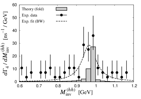
Figure 6: $\pi^{+}\pi^{-}$ invariant mass distribution for the semileptonic decay $D_{s}^{+}\to\pi^{+}\pi^{-}e^{+}\nu_{e}$. The theoretical calculation is folded with the size of experimental bins, $25\text{ MeV}$. The experimental data are taken from Ref. Ecklund:2009aa and are scaled so that the fitted Breit–Wigner distribution (dashed line) reproduces the branching fraction of $\mathcal{B}[D_{s}^{+}\to f_{0}(980)e^{+}\nu_{e},\,f_{0}(980)\to\pi^{+}\pi^{-}]=0.2\%$ by the Particle Data Group (see Table 1).

The theoretical $\pi^{+}\pi^{-}$ mass distribution of the semileptonic decay $D_{s}\to\pi^{+}\pi^{-}e^{+}\nu_{e}$ is compared with the experimental data Ecklund:2009aa in Fig. 6. We note that we plot the figure in unit of $\text{ns}^{-1}/\text{GeV}$, not in arbitrary units. The theoretical mass distribution is folded with $25\text{ MeV}$ spans since the experimental data are collected in bins of $25\text{ MeV}$. The experimental data, on the other hand, are scaled so that the fitted Breit–Wigner distribution reproduces the branching fraction of $\mathcal{B}[D_{s}^{+}\to f_{0}(980)e^{+}\nu_{e},\,f_{0}(980)\to\pi^{+}\pi^{-}]=0.2\%$ Agashe:2014kda . The mass and width of the Breit–Wigner distribution are fixed as $M=966\text{ MeV}$ and $\Gamma=89\text{ MeV}$, respectively, taken from Ref. Ecklund:2009aa . In Fig. 6 we can see a qualitative correspondence between the theoretical and experimental signals of $f_{0}(980)$. We emphasize that, both in experimental and theoretical results, the $\pi^{+}\pi^{-}$ mass distribution shows a clear $f_{0}(980)$ signal while the $f_{0}(500)$ contribution is negligible. This strongly indicates that the $f_{0}(980)$ has a substantial fraction of the strange quarks while the $f_{0}(500)$ has a negligible strange quark component. It is interesting to recall that the appearance of the $f_{0}(980)$ in the case one has a hadronized $s\bar{s}$ component at the end, and no signal of the $f_{0}(500)$, is also observed in $B_{s}^{0}$ and $B^{0}$ decays in Refs. Aaij:2011fx ; Li:2011pg ; Aaltonen:2011nk ; Abazov:2011hv ; LHCb:2012ae . The explanation of this feature along the lines used in the present work was given in Ref. Liang:2014tia . However, although the peak height of the $f_{0}(980)$ is very similar, the Breit–Wigner fit would provide larger branching fraction $\mathcal{B}[D_{s}^{+}\to f_{0}(980)e^{+}\nu_{e}]$ than the theoretical one. Actually, integrating the theoretical mass distribution in the range [$0.9\text{ GeV}$, $1.0\text{ GeV}$], we obtain the branching fraction $\mathcal{B}[D_{s}^{+}\to f_{0}(980)e^{+}\nu_{e};\,f_{0}(980)\to\pi^{+}\pi^{-}]=5.10\times 10^{-4}$, which is about four times smaller than the experimental value $2.00\times 10^{-3}$. Actually, in the experimental analysis of Ref. Ecklund:2009aa different sources of background are considered that make up for the lower mass region of the distribution. The width of the $f_{0}(980)$ extracted in the analysis of Ref. Ecklund:2009aa is $\Gamma=91^{+30}_{-22}\pm 3\text{ MeV}$, which is large compared to most experiments Agashe:2014kda , including the LHCb experiment of Aaij:2014emv , although the admitted uncertainties are also large. One should also take into account that, while a Breit–Wigner distribution for the $f_{0}(980)$ is used in the analysis of Ref. Ecklund:2009aa , the large coupling of the resonance to $K\bar{K}$ requires a Flatte form that brings down fast the $\pi^{+}\pi^{-}$ mass distribution above the $K\bar{K}$ threshold. Our normalization in Fig. 6 is done with the central value of the $\mathcal{B}[D^{+}\to(\pi^{+}K^{-})_{s\text{-wave}}e^{+}\nu_{e}]$ and no extra uncertainties from this branching fraction are considered. Yet, we find instructive to do an exercise, adding to our results a “background” of $10\text{ ns}^{-1}/\text{GeV}$ from different sources that our calculation does not take into account, and then our signal for the $f_{0}(980)$ has a good agreement with the peak of the experimental distribution.

As mentioned above, the value extracted in Ecklund:2009aa for the $f_{0}(980)$ signal is tied to the assumptions made, including parts of the background that lead to a very large width of the resonance, assuming a Breit–Wigner shape, etc. Actually, in a more recent paper Hietala:2015jqa the same CLEO data of Ecklund:2009aa are reanalyzed taking a band of $f_{0}(980)$ masses within $60\text{ MeV}$ of $980\text{ MeV}$ and assuming a Flatte form of the resonance and a rate for $\mathcal{B}[D_{s}^{+}\to f_{0}(980)e^{+}\nu_{e},\,f_{0}(980)\to\pi\pi]=(0.13\pm 0.02\pm 0.01)\%$ is obtained. This value is about a factor of two smaller than the one reported in Ecklund:2009aa and more in agreement with our results.

Figure 7: Differential decay width of the $D_{s}^{+}\to f_{0}(980)e^{+}\nu_{e}$ decay mode followed by $f_{0}(980)\to\pi^{+}\pi^{-}$, with $q^{2}=[M_{\rm inv}^{(l\nu)}]^{2}$. The experimental data are taken from Ref. Ecklund:2009aa . The experimental points should be rescaled dividing by about a factor of two if the absolute rate for the $f_{0}(980)$ production of the reanalysis of Ref. Hietala:2015jqa were used.

Next we consider the differential decay width with respect to the squared momentum transfer $q^{2}$, which coincides with the squared invariant mass of the lepton pair: $q^{2}=[M_{\rm inv}^{(l\nu)}]^{2}$. The differential decay width for the scalar meson production is expressed as

$$\frac{d\Gamma_{4}}{dq^{2}}=\frac{\left|G_{\rm F}\right|^{2}}{64\pi^{5}m_{D}^{3}} \int dM_{\rm inv}^{(hh)}\frac{\left|V_{\rm had}^{(s)}\right|^{2}P_{\rm cm}^{\prime}\tilde{p}_{h}\tilde{p}_{\nu}M_{\rm inv}^{(l\nu)}}{M_{\rm inv}^{(hh)}}$$

$$\times\left(\tilde{E}_{D}\tilde{E}_{S}-\frac{1}{3}|\tilde{\bm{p}}_{D}|^{2}\right).$$ (80)

This differential decay width was experimentally observed in Ref. Ecklund:2009aa for the $D_{s}^{+}\to f_{0}(980)e^{+}\nu_{e}$ decay mode followed by $f_{0}(980)\to\pi^{+}\pi^{-}$. In this study we compare our theoretical value for this decay mode with the experimental data in Fig. 7. The range of the integral for $M_{\rm inv}^{(hh)}$ is [$0.9\text{ GeV}$, $1.0\text{ GeV}$]. As one can see, we can to some extent reproduce the shape of the differential decay width $d\Gamma_{4}/dq^{2}$ in experiment, but the absolute value of the theoretical calculation is several times smaller than the experimental one. This can be, as we have explained, solved by introducing background contributions when extracting the amount of the $f_{0}(980)$ signal from experimental data. Actually, as we have commented before, the reanalysis of Hietala:2015jqa leads to absolute values of the rate for the $f_{0}(980)$ production about a factor of two smaller, and again if we scale the $q^{2}$ distribution of in Fig. 7 by the factor the agreement is much better.

Table 3: Branching fractions of semileptonic $D$ decays into two pseudoscalar mesons in $s$ wave. The branching fraction of the $D^{+}\to(\pi^{+}K^{-})_{s\text{-wave}}e^{+}\nu_{e}$ mode is used as an input.

$D_{s}^{+}$
Mode	Range of $M_{\rm inv}^{(hh)}$ [GeV]	$l=e$	$l=\mu$
$\pi^{+}\pi^{-}$	[0.9, 1.0]	$5.10\times 10^{-4}$	$4.71\times 10^{-4}$
$K^{+}K^{-}$	[$2m_{K}$, 1.2]	$1.42\times 10^{-4}$	$1.30\times 10^{-4}$
$\pi^{-}K^{+}$	[$m_{\pi}+m_{K}$, 1.0]	$8.11\times 10^{-5}$	$7.63\times 10^{-5}$
$D^{+}$
Mode	Range of $M_{\rm inv}^{(hh)}$ [GeV]	$l=e$	$l=\mu$
$\pi^{+}\pi^{-}$	[$2m_{\pi}$, 1.0]	$5.11\times 10^{-4}$	$4.85\times 10^{-4}$
$\pi^{0}\eta$	[$m_{\pi}+m_{\eta}$, 1.1]	$6.37\times 10^{-5}$	$5.86\times 10^{-5}$
$K^{+}K^{-}$	[$2m_{K}$, 1.2]	$2.24\times 10^{-6}$	$2.01\times 10^{-6}$
$\pi^{+}K^{-}$	[$m_{\pi}+m_{K}$, 1.0]	$2.32\times 10^{-3}$	$2.16\times 10^{-3}$
$D^{0}$
Mode	Range of $M_{\rm inv}^{(hh)}$ [GeV]	$l=e$	$l=\mu$
$\pi^{-}\eta$	[$m_{\pi}+m_{\eta}$, 1.1]	$4.93\times 10^{-5}$	$4.53\times 10^{-5}$
$K^{0}K^{-}$	[$2m_{K}$, 1.2]	$5.47\times 10^{-6}$	$4.88\times 10^{-6}$
$\pi^{-}\bar{K}^{0}$	[$m_{\pi}+m_{K}$, 1.0]	$8.99\times 10^{-4}$	$8.38\times 10^{-4}$

Moreover, integrating the mass distributions we calculate the branching fractions of the semileptonic $D$ mesons into two pseudoscalar mesons in $s$ wave, which are listed in Table 3. We note that the branching fraction $\mathcal{B}[D^{+}\to(\pi^{+}K^{-})_{s\text{-wave}}e^{+}\nu_{e}]=2.32\times 10^{-3}$ is used as an input to fix the common constant, $C=4.597$. Among the listed values, we can compare the theoretical and experimental values of the branching fraction $\mathcal{B}[D_{s}^{+}\to(K^{+}K^{-})_{s\text{-wave}}e^{+}\nu_{e}]$. Namely, in Ref. Aubert:2008rs this branching fraction is obtained as $(0.22^{+0.12}_{-0.08}\pm 0.03)\%$ of the total $D_{s}^{+}\to K^{+}K^{-}e^{+}\nu_{e}$, which is dominated by the $\phi(1020)$ vector meson. This indicates, together with the branching fraction $D_{s}^{+}\to\phi(1020)e^{+}\nu_{e}$, we can estimate $\mathcal{B}[D_{s}^{+}\to(K^{+}K^{-})_{s\text{-wave}}e^{+}\nu_{e}]=(5.5^{+3.1}_{-2.1})\times 10^{-5}$. Theoretically this is $1.42\times 10^{-4}$. Although our value overestimates the mean value of the experimental data, it is still in $3\sigma$ errors of the experimental value.

III.2 Production of vector mesons

Table 4: Branching fractions of semileptonic $D$ decays into vector mesons.

$D_{s}^{+}$
Mode	$l=e$	$l=\mu$
$\phi(1020)$	$2.12\times 10^{-2}$	$1.94\times 10^{-2}$
$K^{\ast}(892)^{0}$	$2.02\times 10^{-3}$	$1.89\times 10^{-3}$
$D^{+}$
Mode	$l=e$	$l=\mu$
$\bar{K}^{\ast}(892)^{0}$	$5.56\times 10^{-2}$	$5.12\times 10^{-2}$
$\rho(770)^{0}$	$2.54\times 10^{-3}$	$2.37\times 10^{-3}$
$\omega(782)$	$2.46\times 10^{-3}$	$2.29\times 10^{-3}$
$D^{0}$
Mode	$l=e$	$l=\mu$
$K^{\ast}(892)^{-}$	$2.15\times 10^{-2}$	$1.98\times 10^{-2}$
$\rho(770)^{-}$	$1.97\times 10^{-3}$	$1.84\times 10^{-3}$

Let us move to the vector meson productions in the semileptonic $D$ decays. For the vector mesons we fix the common prefactor $C^{\prime}$ so as to reproduce the 10 available experimental branching fractions listed in Table 1. From the best fit we obtain the value $C^{\prime}=1.563\text{ GeV}$, which gives $\chi^{2}/N_{\rm d.o.f.}=22.8/9\approx 2.53$. The theoretical values of the branching fractions are listed in Table 4 and are compared with the experimental data in Fig. 8, where we plot the ratio of the experimental to theoretical branching fractions. We calculate the experimental branching fraction of the $D^{+}\to\bar{K}(892)^{0}l^{+}\nu_{l}$ ($l=e$ and $\mu$) process by dividing the value in Table 1 by the branching fraction $\mathcal{B}[\bar{K}^{\ast}(892)^{0}\to K^{-}\pi^{+}]=2/3$, which is obtained with isospin symmetry. As one can see from Fig. 8, the experimental values are reproduced well solely by the model parameter $C^{\prime}$ with $\chi^{2}/N_{\rm d.o.f.}\approx 2.53$.

Figure 8: Ratio of the experimental to theoretical branching fractions for the semileptonic $D$ decays into vector mesons.

Figure 9: Differential decay width of the $D_{s}^{+}\to\phi(1020)e^{+}\nu_{e}$ decay mode followed by $\phi(1020)\to K^{+}K^{-}$, with $q^{2}=[M_{\rm inv}^{(l\nu)}]^{2}$. The experimental data are taken from Ref. Ecklund:2009aa . The theoretical value is multiplied by the branching fraction of the $\phi(1020)$ meson to $K^{+}K^{-}$, $\mathcal{B}[\phi(1020)\to K^{+}K^{-}]=48.9\%$ Agashe:2014kda .

Next for the $D_{s}^{+}\to\phi(1020)e^{+}\nu_{e}$ decay mode we consider the differential decay width with respect to the squared momentum transfer $q^{2}$, which coincides with the squared invariant mass of the lepton pair: $q^{2}=[M_{\rm inv}^{(l\nu)}]^{2}$. This differential decay width was already measured in an experiment Ecklund:2009aa for the $D_{s}^{+}\to\phi(1020)e^{+}\nu_{e}$ decay mode. In a similar manner to the previous case, the differential decay width for the vector meson production is expressed as

$$\frac{d\Gamma_{3}}{dq^{2}}=\frac{\left|G_{\rm F}V_{\rm had}^{(v)}\right|^{2}}{16\pi^{3}m_{D}^{3}m_{V}}P_{\rm cm}\tilde{p}_{\nu}M_{\rm inv}^{(l\nu)}\left(\tilde{E}_{D}\tilde{E}_{V}-\frac{1}{3}|\tilde{\bm{p}}_{D}|^{2}\right).$$ (81)

In Fig. 9 we compare our result for this reaction with the experimental one. As one can see, our theoretical result reproduces the experimental value of the differential decay width quantitatively well. This means that our method to calculate the semileptonic decays of $D$ mesons is good enough to describe the decays into vector mesons.

In this study we have not evaluated the $D^{+}\to\phi(1020)e^{+}\nu_{e}$ decay. This decay proceeds like the $D^{+}\to\omega(782)e^{+}\nu_{e}$ decay that we have evaluated and one has a $d\bar{d}$ at the end. Since the $\phi$ is $s\bar{s}$ then this is forbidden in our approach, at the tree level that we have considered for the vector production. Experimentally, this rate is $<9\times 10^{-5}$. This is an upper bound about $30$ times smaller than the rate of the omega production that we have evaluated. We do not want to go beyond, but can give some idea on how a finite rate could be obtained in our approach. For this one would have to hadronize the $d\bar{d}$ into a $K^{0}\bar{K}^{0}$, then have a loop for $K^{0}\bar{K}^{0}$ propagation in $p$-wave and finally have the $K^{0}\bar{K}^{0}$ couple to the $\phi$. Some technical details could be borrowed from the study of $\phi\to\pi\pi$ decay studied in Oller:1999ag but one can get an indication that the rate should be rather small by simply noting that the hadronization to meson–meson pairs has a reduction factor, as one can see by comparing for instance $f_{0}(500)$ production with $\rho$ production Bayar:2014qha . On the other hand, the coupling of $\phi$ to $K^{0}\bar{K}^{0}$ is intrinsically small, as one can see from the $1.5\text{ MeV}$ partial decay width of this channel [comparatively the $\Delta(1232)$ partial decay width to the $\pi N$ channel would be about $15\text{ MeV}$ for a pion with the same momentum as the kaon in the $\phi$ decay]. There are other factors to consider, but this can give us a feeling that the rate could be some orders of magnitude smaller than for omega production.

III.3 Comparison between scalar and vector meson contributions

Finally we compare the mass distributions of the two pseudoscalar mesons in $s$- and $p$-wave contributions. In the present approach the $s$-wave part comes from the rescattering of two pseudoscalar mesons including the scalar meson contribution, while the $p$-wave one from the decay of a vector meson. In this study we consider three decay modes: $D_{s}^{+}\to\pi^{+}\pi^{-}e^{+}\nu_{e}$, $D_{s}^{+}\to K^{+}K^{-}e^{+}\nu_{e}$, and $D^{+}\to\pi^{+}K^{-}e^{+}\nu_{e}$. The $D^{+}\to\pi^{+}\pi^{-}e^{+}\nu_{e}$ decay mode would have a large $p$-wave contribution from $\rho(770)$, but we do not consider this decay mode since it is a Cabibbo suppressed process.

First we consider the $D_{s}^{+}\to\pi^{+}\pi^{-}e^{+}\nu_{e}$ decay mode. This is a specially clean mode, since it does not have vector meson contributions and is dominated by the $s$-wave part. Namely, while the $\pi^{+}\pi^{-}$ can come from a scalar meson, the primary quark–antiquark pair in the semileptonic $D_{s}^{+}$ decay is $s\bar{s}$, which is isospin $I=0$ and hence the $\rho(770)$ cannot contribute to the $\pi^{+}\pi^{-}$ mass distribution. The primary $s\bar{s}$ can be $\phi(1020)$, but it decays dominantly to $K\bar{K}$ and the $\phi(1020)\to\pi^{+}\pi^{-}$ decay is negligible. This fact enables us to observe the scalar meson peak without a contamination from vector meson decays and discuss the quark configuration in the $f_{0}(980)$ resonance as in Sec. III.1.

Figure 10: $K^{+}K^{-}$ invariant mass distribution for the semileptonic decay $D_{s}^{+}\to K^{+}K^{-}e^{+}\nu_{e}$ both in $s$ and $p$ waves.

Next let us consider the $D_{s}^{+}\to K^{+}K^{-}e^{+}\nu_{e}$ decay mode. As we have seen, the $K^{+}K^{-}$ mass distribution in $s$ wave is a consequence of the $f_{0}(980)$ tail. However, its contribution should be largely contaminated by the $\phi(1020)\to K^{+}K^{-}$ in $p$ wave, which has a larger branching fraction than the $(K^{+}K^{-})_{s\text{-wave}}$ in the semileptonic decay. In order to see this, we calculate the $p$-wave $K^{+}K^{-}$ mass distribution for $D_{s}^{+}\to K^{+}K^{-}e^{+}\nu_{e}$, which can be formulated as

$$\frac{d\Gamma_{3}}{dM_{\rm inv}^{(hh)}}=-\frac{2m_{V}}{\pi}\text{Im }\frac{\Gamma_{3}\times\mathcal{B}[V\to hh]}{[M_{\rm inv}^{(hh)}]^{2}-m_{V}^{2}+im_{V}\Gamma_{V}(M_{\rm inv}^{(hh)})},$$ (82)

where $m_{V}$ is the vector meson mass and the energy dependent decay width $\Gamma_{V}(M_{\rm inv}^{(hh)})$ is defined as

$$\Gamma_{V}(M_{\rm inv}^{(hh)})\equiv\bar{\Gamma}_{V}\left(\frac{p^{\rm off}(M_{\rm inv}^{(hh)})}{p^{\rm on}}\right)^{3},$$ (83)

$$p^{\rm off}(M_{\rm inv}^{(hh)})\equiv\frac{\lambda^{1/2}([M_{\rm inv}^{(hh)}]^{2},\,m_{h}^{2},\,m_{h}^{\prime 2})}{2M_{\rm inv}^{(hh)}},$$ (84)

$$p^{\rm on}\equiv\frac{\lambda^{1/2}(m_{V}^{2},\,m_{h}^{2},\,m_{h}^{\prime 2})}{2m_{V}}.$$ (85)

For the $\phi(1020)$ meson we take $\bar{\Gamma}_{\phi}=4.27\text{ MeV}$ and $\mathcal{B}[\phi\to K^{+}K^{-}]=0.489$ Agashe:2014kda . The numerical result for the $(K^{+}K^{-})_{p\text{-wave}}$ mass distribution is shown in Fig. 10 together with the $(K^{+}K^{-})_{s\text{-wave}}$. From the figure, compared to the $(K^{+}K^{-})_{p\text{-wave}}$ contribution we cannot find any significant $(K^{+}K^{-})_{s\text{-wave}}$ contribution, which was already noted in the experimental mass distribution in Ref. Aubert:2008rs . Nevertheless, we emphasize that the $(K^{+}K^{-})_{s\text{-wave}}$ fraction of the semileptonic $D_{s}^{+}$ decay is large enough to be extracted Aubert:2008rs . Actually in Ref. Aubert:2008rs they extracted the $(K^{+}K^{-})_{s\text{-wave}}$ fraction by analysing the interference between the $s$- and $p$-wave contributions. This fact, and the qualitative reproduction of the branching fractions in our model, implies that the $f_{0}(980)$ resonance couples to the $K\bar{K}$ channel with a certain strength, which can be translated into the $K\bar{K}$ component in $f_{0}(980)$, in a similar manner to the $KD$ component in $D_{s0}^{\ast}(2317)$ Albaladejo:2015kea ; Navarra:2015iea , in terms of the compositeness Sekihara:2014kya . Anyway, in order to conclude the structure of the $f_{0}(980)$ more clearly, it is important to reduce the experimental errors on the $(K^{+}K^{-})_{s\text{-wave}}$.

Figure 11: $\pi^{+}K^{-}$ invariant mass distribution for the semileptonic decay $D^{+}\to\pi^{+}K^{-}e^{+}\nu_{e}$ both in $s$ and $p$ waves.

Finally we consider the $D^{+}\to\pi^{+}K^{-}e^{+}\nu_{e}$ decay mode. In this mode the $(\pi^{+}K^{-})_{s\text{-wave}}$ from the $K_{0}^{\ast}(800)$ and the $(\pi^{+}K^{-})_{p\text{-wave}}$ from the $K^{\ast}(892)$ are competing with each other. In a similar manner to the $D_{s}^{+}\to K^{+}K^{-}e^{+}\nu_{e}$ case, we calculate the mass distribution also for the $p$-wave $\pi^{+}K^{-}$ contribution $d\Gamma_{3}/dM_{\rm inv}^{(hh)}$ with $\bar{\Gamma}_{K^{\ast}}=49.1\text{ MeV}$ Agashe:2014kda , and the result is shown in Fig. 11. As one can see, thanks to the width of $\sim 50\text{ MeV}$ for the $K^{\ast}(892)$, the $s$-wave component can dominate the mass distribution below $0.8\text{ GeV}$. We note that we would obtain an almost similar result for the $D^{0}\to\pi^{-}\bar{K}^{0}e^{+}\nu_{e}$ decay mode due to isospin symmetry.

As to the theoretical uncertainties, we can play a bit with the cut-offs used to regularize the loops, such that the masses of the states do not change appreciably. This exercise has been done a number of times and given us the feeling that within our models the uncertainties are below $10\%$. For the case of scalar production where we have a range of invariant masses and rely upon a constant production vertex $C$, the changes with the invariant mass in the primary form factors, prior to the final state interaction of the mesons, as found in Kang:2013jaa , would add some extra uncertainty. In total it would be fair to accept about $20\%$ uncertainties in this case in the limited range of energies that we move.

IV Conclusion

In this study we have discussed the semileptonic decays of $D$ mesons into light scalar and vector mesons. For the scalar meson production, we have formulated the semileptonic decay as the combination of two parts. One is the weak decay of the charm quark and the emission of a lepton pair via the $W$ boson. The other is a simple hadronization of light $q\bar{q}$ pair plus an extra $\bar{q}q$ from vacuum into two pseudoscalar mesons after the $W$ boson emission, so as to generate the scalar mesons dynamically in the meson–meson final state interaction. The hadronization naturally gives the weight of each pair of pseudoscalar mesons in the decay process, which governs which scalar meson appears in the decay mode. For the vector mesons, on the other hand, we have not considered the hadronization with an extra $\bar{q}q$ and have directly used the light $q\bar{q}$ pair after the $W$ boson emission as a weight for the vector mesons, which are expected to be genuinely $q\bar{q}$ states. We note that we can specify flavors of quarks contained in the final state scalar and vector mesons by considering Cabibbo favored and suppressed processes. In addition, since the leptons interact only weakly, the semileptonic decay of the heavy meson to two light mesons $+l^{+}\nu_{l}$ brings a suitable condition to measure effects of the final state interaction of the two light mesons.

In our model of the semileptonic decay, the production yields of the scalar and vector mesons are respectively determined solely by constant prefactors $C$ and $C^{\prime}$ as model parameters. Fixing $C$ from the branching fraction of the $D^{+}\to(\pi^{+}K^{-})_{s\text{-wave}}e^{+}\nu_{e}$ decay, we have calculated branching fractions of scalar meson productions. We have qualitatively reproduced the experimental value of the branching fractions of $D_{s}^{+}\to(\pi^{+}\pi^{-})_{s\text{-wave}}e^{+}\nu_{e}$ and $(K^{+}K^{-})_{s\text{-wave}}e^{+}\nu_{e}$ decay modes. Some deviations of these branching fractions compared to the experimental values can be explained by taking into account the background of the mass distribution for the $\pi^{+}\pi^{-}$ case and by the large experimental error for the $K^{+}K^{-}$ case. For the vector mesons, we have determined the constant $C^{\prime}$ so as to fit our numerical values to the available experimental values of the branching fractions, and we have reproduced the experimental values at a quantitative level. We also compared the mass distributions of the two pseudoscalar mesons in $s$- and $p$-wave contributions, which come from decays of the scalar and vector mesons, respectively.

We have found that the Cabibbo favored decay mode $D_{s}^{+}\to f_{0}(980)l^{+}\nu_{l}$ followed by $f_{0}(980)\to\pi^{+}\pi^{-}$ and $K^{+}K^{-}$ is of special interest. For the $f_{0}(980)\to\pi^{+}\pi^{-}$ mode, we have found that there is no $p$-wave contamination from $\rho(770)$ decay and hence it should be dominated by the $s$-wave part. Then, we have confirmed the experimental fact that the $\pi^{+}\pi^{-}$ mass distribution shows a clear $f_{0}(980)$ signal while the $f_{0}(500)$ contribution is negligible. This strongly indicates that the $f_{0}(980)$ has a substantial fraction of the strange quarks while the $f_{0}(500)$ has a negligible strange quark component. For the $f_{0}(980)\to K^{+}K^{-}$ mode, on the other hand, the $(K^{+}K^{-})_{s\text{-wave}}$ contribution is highly contaminated by the $\phi(1020)\to K^{+}K^{-}$ decay in $p$ wave. Nevertheless, the $(K^{+}K^{-})_{s\text{-wave}}$ fraction of the semileptonic $D_{s}^{+}$ decay is large enough to be extracted experimentally, which implies that the $f_{0}(980)$ resonance couples to the $K\bar{K}$ channel with a certain strength and hence implies a certain amount of the $K\bar{K}$ component in $f_{0}(980)$.

Appendix A Conventions

In this Appendix we summarize conventions used in this study.

A.1 Metric and Lorentz indices

In this article the metric in four-dimensional Minkowski space is $g^{\mu\nu}=g_{\mu\nu}=\text{diag}(1,\,-1,\,-1,\,-1)$ and the Einstein summation convention is used unless explicitly mentioned. The scalar product of two vectors $a^{\mu}$ and $b^{\mu}$ is represented as $a\cdot b=a_{\mu}b^{\mu}=a^{0}b^{0}-\bm{a}\cdot\bm{b}$.

A.2 Dirac spinors and matrices

As the positive and negative energy solutions of the Dirac equation, we express the Dirac spinors respectively as $u(\bm{p},\,s)$ and $v(\bm{p},\,s)$, where $\bm{p}$ is three-momentum of the field and $s$ represents its spin. The Dirac spinors are normalized as follows:

$$\overline{u}(\bm{p},\,s)u(\bm{p},\,s^{\prime})=\delta_{ss^{\prime}},\quad\overline{v}(\bm{p},\,s)v(\bm{p},\,s^{\prime})=-\delta_{ss^{\prime}},$$ (86)

with $\overline{u}\equiv u^{\dagger}\gamma^{0}$ and $\overline{v}\equiv v^{\dagger}\gamma^{0}$, and hence we have

$$\begin{split}&\sum_{s}u(\bm{p},\,s)\overline{u}(\bm{p},\,s)=\frac{\ooalign{\hfil/\hfil\crcr$p$}+m}{2m},\\ &\sum_{s}v(\bm{p},\,s)\overline{v}(\bm{p},\,s)=\frac{\ooalign{\hfil/\hfil\crcr$p$}-m}{2m},\end{split}$$ (87)

where $m$ is the mass of the field, $\ooalign{\hfil/\hfil\crcr$p$}\equiv\gamma^{\mu}p_{\mu}$ with $\gamma^{\mu}$ being the Dirac $\gamma$ matrices, and $p^{\mu}\equiv\left(\sqrt{\bm{p}^{2}+m^{2}},\,\bm{p}\right)$ is the on-shell four-momentum of the solution.

The identities for the Dirac matrices used in this study are summarized as follows:

$$\gamma^{0}(\gamma^{\mu})^{\dagger}\gamma^{0}=\gamma^{\mu},\quad(\gamma_{5})^{\dagger}=\gamma_{5},$$ (88)

$$\text{tr}\left[\gamma^{\mu}\gamma^{\nu}\gamma^{\rho}\gamma^{\sigma}\right]=4(g^{\mu\nu}g^{\rho\sigma}-g^{\mu\rho}g^{\nu\sigma}+g^{\mu\sigma}g^{\nu\rho}),$$ (89)

$$\text{tr}\left[\gamma_{5}\gamma^{\mu}\gamma^{\nu}\gamma^{\rho}\gamma^{\sigma}\right]=-4i\epsilon^{\mu\nu\rho\sigma},$$ (90)

$$\text{tr}\left[\gamma^{\mu}\gamma^{\nu}\gamma^{\rho}\right]=\text{tr}\left[\gamma_{5}\gamma^{\mu}\gamma^{\nu}\gamma^{\rho}\right]=0,$$ (91)

where $\gamma_{5}\equiv i\gamma^{0}\gamma^{1}\gamma^{2}\gamma^{3}$ and $\epsilon^{\mu\nu\rho\sigma}$ is the Levi-Civita symbol with the normalization $\epsilon^{0123}=1$. The Levi-Civita symbol satisfies the following identity

$$\epsilon^{\alpha\beta\mu\nu}\epsilon_{\alpha\beta\rho\sigma}=-2(g^{\mu}_{\rho}g^{\nu}_{\sigma}-g^{\mu}_{\sigma}g^{\nu}_{\rho}).$$ (92)

A.3 Isospin basis

In terms of the isospin states $|I,\,I_{3}\rangle$, the phase convention for pseudoscalar mesons is given by

$$|\pi^{+}\rangle=-|1,\,1\rangle,\quad|K^{-}\rangle=-|1/2,\,-1/2\rangle,$$ (93)

while other pseudoscalar mesons are represented without phase factors. As a result, we can translate the physical two-pseudoscalar meson states into the isospin basis, which we specify as $(I,\,I_{3})$, as

$$|K\bar{K}(0,\,0)\rangle=-\frac{1}{\sqrt{2}}|K^{+}K^{-}\rangle-\frac{1}{\sqrt{2}}|K^{0}\bar{K}^{0}\rangle,$$ (94)

$$|\eta\eta(0,\,0)\rangle=|\eta\eta\rangle,$$ (95)

$$|K\bar{K}(1,\,0)\rangle=-\frac{1}{\sqrt{2}}|K^{+}K^{-}\rangle+\frac{1}{\sqrt{2}}|K^{0}\bar{K}^{0}\rangle,$$ (96)

$$|K\bar{K}(1,\,-1)\rangle=-|K^{0}K^{-}\rangle,$$ (97)

$$|\pi\eta(1,\,0)\rangle=|\pi^{0}\eta\rangle,$$ (98)

$$|\pi\eta(1,\,-1)\rangle=|\pi^{-}\eta\rangle,$$ (99)

$$|\pi K(1/2,\,-1/2)\rangle=\frac{1}{\sqrt{3}}|\pi^{0}K^{0}\rangle-\sqrt{\frac{2}{3}}|\pi^{-}K^{+}\rangle,$$ (100)

$$|\pi\bar{K}(1/2,\,1/2)\rangle=\sqrt{\frac{2}{3}}|\pi^{+}K^{-}\rangle-\frac{1}{\sqrt{3}}|\pi^{0}\bar{K}^{0}\rangle,$$ (101)

$$|\pi\bar{K}(1/2,\,-1/2)\rangle=-\frac{1}{\sqrt{3}}|\pi^{0}K^{-}\rangle-\sqrt{\frac{2}{3}}|\pi^{-}\bar{K}^{0}\rangle,$$ (102)

Furthermore, the vector meson states are represented in terms of quarks as

$$|\rho^{0}\rangle=\frac{1}{\sqrt{2}}|u\bar{u}\rangle-\frac{1}{\sqrt{2}}|d\bar{d}\rangle,\quad|\rho^{-}\rangle=|d\bar{u}\rangle,$$ (103)

$$|\omega\rangle=\frac{1}{\sqrt{2}}|u\bar{u}\rangle+\frac{1}{\sqrt{2}}|d\bar{d}\rangle,$$ (104)

$$|K^{\ast 0}\rangle=|d\bar{s}\rangle,\quad|\bar{K}^{\ast 0}\rangle=|s\bar{d}\rangle,\quad|\bar{K}^{\ast-}\rangle=-|s\bar{u}\rangle.$$ (105)

A.4 Feynman rules

The $W\nu l$ coupling is expressed as

$$-iV_{W\nu l}^{\mu}=i\frac{g_{\rm W}}{\sqrt{2}}\gamma^{\mu}\frac{1-\gamma_{5}}{2},$$ (106)

with $g_{\rm W}$ being the coupling constant of the weak interaction, and the $Wcq$ coupling as

$$-iV_{Wcq}^{\mu}=i\frac{g_{\rm W}V_{cq}}{\sqrt{2}}\gamma^{\mu}\frac{1-\gamma_{5}}{2},$$ (107)

where $V_{cq}$ is the Cabibbo–Kobayashi–Maskawa matrix elements for the transition from the charm to light quark $q$. The $W$ boson propagator with four-momentum $p^{\mu}$ is written as

$$iP_{W}^{\mu\nu}(p)=\frac{-ig^{\mu\nu}}{p^{2}-M_{W}^{2}+i0},$$ (108)

with the mass of the $W$ boson $M_{W}$. The coupling constant $g_{\rm W}$ and the mass of the $W$ boson $M_{W}$ are related to the Fermi coupling constant $G_{\rm F}$ as

$$G_{\rm F}=\frac{g_{\rm W}^{2}}{4\sqrt{2}M_{W}^{2}}.$$ (109)

A.5 Physical constants

In this article we use the following values for physical constants. The Fermi coupling constant: $G_{\rm F}\approx 1.166\times 10^{-5}\text{ GeV}^{-2}$. The Cabibbo–Kobayashi–Maskawa matrix elements: $|V_{cs}|\approx 0.986$ and $|V_{cd}|\approx 0.225$. The masses of heavy mesons: $m_{D_{s}^{+}}=1968.30\text{ MeV}$, $m_{D^{+}}=1869.61\text{ MeV}$, and $m_{D^{0}}=1864.84\text{ MeV}$. Isospin symmetric masses are used for the light mesons: $m_{\pi}=138.04\text{ MeV}$, $m_{K}=495.67\text{ MeV}$, and $m_{\eta}=547.85\text{ MeV}$ for the pseudoscalar mesons, and $m_{\rho}=775.19\text{ MeV}$, $m_{\omega}=782.65\text{ MeV}$, $m_{K^{\ast}}=893.74\text{ MeV}$, and $m_{\phi}=1019.46\text{ MeV}$ for the vector mesons. The masses of the leptons: $m_{e}=0.511\text{ MeV}$, $m_{\mu}=105.66\text{ MeV}$, and $m_{\nu_{e}}=m_{\nu_{\mu}}=0\text{ MeV}$.

References

- (1) K. A. Olive et al. [Particle Data Group Collaboration], Chin. Phys. C 38, 090001 (2014).
- (2) R. Aaij et al. [LHCb Collaboration], Phys. Lett. B 698, 115 (2011).
- (3) J. Li et al. [Belle Collaboration], Phys. Rev. Lett. 106, 121802 (2011).
- (4) T. Aaltonen et al. [CDF Collaboration], Phys. Rev. D 84, 052012 (2011).
- (5) V. M. Abazov et al. [D0 Collaboration], Phys. Rev. D 85, 011103 (2012).
- (6) R. Aaij et al. [LHCb Collaboration], Phys. Rev. D 86, 052006 (2012).
- (7) W. H. Liang and E. Oset, Phys. Lett. B 737, 70 (2014).
- (8) J. A. Oller and E. Oset, Nucl. Phys. A 620, 438 (1997) [Erratum-ibid. A 652, 407 (1999)].
- (9) N. Kaiser, Eur. Phys. J. A 3, 307 (1998).
- (10) M. P. Locher, V. E. Markushin and H. Q. Zheng, Eur. Phys. J. C 4, 317 (1998).
- (11) J. A. Oller, E. Oset and J. R. Pelaez, Phys. Rev. Lett. 80, 3452 (1998).
- (12) J. A. Oller, E. Oset and J. R. Pelaez, Phys. Rev. D 59, 074001 (1999) [Erratum-ibid. D 60, 099906 (1999)] [Erratum-ibid. D 75, 099903 (2007)].
- (13) J. A. Oller and E. Oset, Phys. Rev. D 60, 074023 (1999).
- (14) J. Nieves and E. Ruiz Arriola, Nucl. Phys. A 679, 57 (2000).
- (15) J. R. Pelaez and G. Rios, Phys. Rev. Lett. 97, 242002 (2006).
- (16) M. Albaladejo and J. A. Oller, Phys. Rev. Lett. 101, 252002 (2008).
- (17) A. Martinez Torres, L. S. Geng, L. R. Dai, B. X. Sun, E. Oset and B. S. Zou, Phys. Lett. B 680, 310 (2009).
- (18) J. J. Xie, L. R. Dai and E. Oset, Phys. Lett. B 742, 363 (2015).
- (19) F. S. Navarra, M. Nielsen, E. Oset and T. Sekihara, Phys. Rev. D 92, no. 1, 014031 (2015).
- (20) M. Ablikim et al. [BES Collaboration], Eur. Phys. J. C 47, 31 (2006).
- (21) M. Ablikim et al. [BES Collaboration], Eur. Phys. J. C 47, 39 (2006).
- (22) J. M. Link et al. [FOCUS Collaboration], Phys. Lett. B 598, 33 (2004).
- (23) J. M. Link et al. [FOCUS Collaboration], Phys. Lett. B 637, 32 (2006).
- (24) B. Aubert et al. [BaBar Collaboration], Phys. Rev. D 78, 051101 (2008).
- (25) P. del Amo Sanchez et al. [BaBar Collaboration], Phys. Rev. D 83, 072001 (2011).
- (26) J. Yelton et al. [CLEO Collaboration], Phys. Rev. D 80, 052007 (2009).
- (27) K. M. Ecklund et al. [CLEO Collaboration], Phys. Rev. D 80, 052009 (2009).
- (28) L. Martin et al. [CLEO Collaboration], Phys. Rev. D 84, 012005 (2011).
- (29) J. Yelton et al. [CLEO Collaboration], Phys. Rev. D 84, 032001 (2011)
- (30) S. Dobbs et al. [CLEO Collaboration], Phys. Rev. Lett. 110, no. 13, 131802 (2013).
- (31) I. Bediaga, F. S. Navarra and M. Nielsen, Phys. Lett. B 579, 59 (2004).
- (32) H. W. Ke, X. Q. Li and Z. T. Wei, Phys. Rev. D 80, 074030 (2009).
- (33) N. N. Achasov and A. V. Kiselev, Phys. Rev. D 86, 114010 (2012).
- (34) A. H. Fariborz, R. Jora, J. Schechter and M. Naeem Shahid, Phys. Rev. D 84, 094024 (2011).
- (35) A. H. Fariborz, R. Jora, J. Schechter and M. N. Shahid, Int. J. Mod. Phys. A 30, no. 02, 1550012 (2015).
- (36) W. Wang and C. D. Lu, Phys. Rev. D 82, 034016 (2010).
- (37) U. G. Meissner and W. Wang, Phys. Lett. B 730, 336 (2014).
- (38) W. Wang and R. L. Zhu, Phys. Lett. B 743, 467 (2015).
- (39) U. G. Meissner and W. Wang, JHEP 1401, 107 (2014).
- (40) W. F. Wang, H. n. Li, W. Wang and C. D. Lu, Phys. Rev. D 91, no. 9, 094024 (2015).
- (41) X. W. Kang, B. Kubis, C. Hanhart and U. G. Meissner, Phys. Rev. D 89, 053015 (2014).
- (42) M. Doring, U. G. Meissner and W. Wang, JHEP 1310, 011 (2013).
- (43) Y. J. Shi and W. Wang, arXiv:1507.07692 [hep-ph].
- (44) A. Bramon, A. Grau and G. Pancheri, Phys. Lett. B 283, 416 (1992).
- (45) A. V. Manohar and M. B. Wise, “Heavy quark physics,” Camb. Monogr. Part. Phys. Nucl. Phys. Cosmol. 10, 1 (2000).
- (46) R. Aaij et al. [LHCb Collaboration], Phys. Rev. D 89, no. 9, 092006 (2014).
- (47) J. Hietala, D. Cronin-Hennessy, T. Pedlar and I. Shipsey, Phys. Rev. D 92, no. 1, 012009 (2015).
- (48) J. A. Oller, E. Oset and J. R. Pelaez, Phys. Rev. D 62, 114017 (2000).
- (49) M. Bayar, W. H. Liang and E. Oset, Phys. Rev. D 90, no. 11, 114004 (2014).
- (50) M. Albaladejo, M. Nielsen and E. Oset, Phys. Lett. B 746, 305 (2015).
- (51) T. Sekihara, T. Hyodo and D. Jido, PTEP 2015, no. 6, 063D04.