A Bayesian Approach for Online Classifier Ensemble

Abstract

We propose a Bayesian approach for recursively estimating the classifier weights in online learning of a classifier ensemble. In contrast with past methods, such as stochastic gradient descent or online boosting, our approach estimates the weights by recursively updating its posterior distribution. For a specified class of loss functions, we show that it is possible to formulate a suitably defined likelihood function and hence use the posterior distribution as an approximation to the global empirical loss minimizer. If the stream of training data is sampled from a stationary process, we can also show that our approach admits a superior rate of convergence to the expected loss minimizer than is possible with standard stochastic gradient descent. In experiments with real-world datasets, our formulation often performs better than state-of-the-art stochastic gradient descent and online boosting algorithms.

Keywords: Online learning, classifier ensembles, Bayesian methods.

1 Introduction

The basic idea of classifier ensembles is to enhance the performance of individual classifiers by combining them. In the offline setting, a popular approach to obtain the ensemble weights is to minimize the training error, or a surrogate risk function that approximates the training error. Solving this optimization problem usually calls for various sorts of gradient descent methods. For example, the most successful and popular ensemble technique, boosting, can be viewed in such a way (Freund and Schapire, 1995; Mason et al., 1999; Friedman, 2001; Telgarsky, 2012). Given the success of these ensemble techniques in a variety of batch learning tasks, it is natural to consider extending this idea to the online setting, where the labeled sample pairs $\{\mathbf{x}_{t},y_{t}\}_{t=1}^{T}$ are presented to and processed by the algorithm sequentially, one at a time.

Indeed, online versions of ensemble methods have been proposed from a spectrum of perspectives. Some of these works focus on close approximation of offline ensemble schemes, such as boosting (Oza and Russell, 2001; Pelossof et al., 2009). Other methods are based on stochastic gradient descent (Babenko et al., 2009b; Leistner et al., 2009; Grbovic and Vucetic, 2011). Recently, Chen et al. (2012) formulated a smoothed boosting algorithm based on the analysis of regret from offline benchmarks. Despite their success in many applications (Grabner and Bischof, 2006; Babenko et al., 2009a), however, there are some common drawbacks of these online ensemble methods, including the lack of a universal framework for theoretical analysis and comparison, and the ad hoc tuning of learning parameters such as step size.

In this work, we propose an online ensemble classification method that is not based on boosting or gradient descent. The main idea is to recursively estimate a posterior distribution of the ensemble weights in a Bayesian manner. We show that, for a given class of loss functions, we can define a likelihood function on the ensemble weights and, with an appropriately formulated prior distribution, we can generate a posterior mean that closely approximates the empirical loss minimizer. If the stream of training data is sampled from a stationary process, this posterior mean converges to the expected loss minimizer.

Let us briefly explain the rationale for this scheme, which shall be contrasted from the usual Bayesian setup where the likelihood is chosen to describe closely the generating process of the training data. In our framework, we view Bayesian updating as a loss minimization procedure: it provides an approximation to the minimizer of a well-defined risk function. More precisely, this risk minimization interpretation comes from the exploitation of two results in statistical asymptotic theory. First is that, under mild regularity conditions, a Bayesian posterior distribution tends to peak at the maximum likelihood estimate (MLE) of the same likelihood function, as a consequence of the so-called Laplace method (MacKay, 2003). Second, MLE can be viewed as a risk minimizer, where the risk is defined precisely as the expected negative log-likelihood. Therefore, given a user-defined loss function, one can choose a suitable log-likelihood as a pure artifact, and apply a corresponding Bayesian update to minimize the risk. We will develop the theoretical foundation that justifies the above rationale.

Our proposed online ensemble classifier learning scheme is straightforward, but powerful in two respects. First, whenever our scheme is applicable, it can approximate the global optimal solution, in contrast with local methods such as stochastic gradient descent (SGD). Second, assuming the training data is sampled from a stationary process, our proposed scheme possesses a rate of convergence to the expected loss minimizer that is at least as fast as standard SGD. In fact, our rate is faster unless the SGD step size is chosen optimally, which cannot be done a priori in the online setting. Furthermore, we also found that our method performs better in experiments with finite datasets compared with the averaging schemes in SGD (Polyak and Juditsky, 1992; Schmidt et al., 2013) that have the same optimal theoretical convergence rate as our method.

In addition to providing a theoretical analysis of our formulation, we also tested our approach on real-world datasets and compared with individual classifiers, a baseline stochastic gradient descent method for learning classifier ensembles, and their averaging variants, as well as state-of-the-art online boosting methods. We found that our scheme consistently achieves superior performance over the baselines and often performs better than state-of-the-art online boosting algorithms, further demonstrating the validity of our theoretical analysis.

In summary, our contributions are:

1. We propose a Bayesian approach to estimate the classifier weights with closed-form updates for online learning of classifier ensembles.

2. We provide theoretical analyses of both the convergence guarantee and the bound on prediction error.

3. We compare the asymptotic convergence rate of the proposed framework versus previous gradient descent frameworks thereby demonstrating the advantage of the proposed framework.

This paper is organized as follows. We first briefly discuss the related works. We then state in detail our approach and provide theoretical guarantees in Section 3. A specific example for solving the online ensemble problem is provided in Section 4, and numerical experiments are reported in Section 5. We discuss the use of other loss functions for online ensemble learning in Section 6 and conclude our paper in Section 7 with future work. Some technical proofs are left to the Appendix.

2 Related work

There is considerable past work on online ensemble learning. Many past works have focused on online learning with concept drift (Wang et al., 2003; Kolter and Maloof, 2005, 2007; Minku, 2011), where dynamic strategies of pruning and rebuilding ensemble members are usually considered. Given the technical difficulty, theoretical analysis for concept drift seems to be underdeveloped. Kolter and Maloof (2005) proved error bounds for their proposed method, which appears to be the first such theoretical analysis, yet such analysis is not easily generalized to other methods in this category. Other works, such as Schapire (2001), and Cesa-Bianchi and Lugosi (2003), obtained performance bounds from the perspective of iterative games.

Our work is more closely related to methods that operate in a stationary environment, most notably some online boosting methods. One of the first methods was proposed by Oza and Russell (2001), who showed asymptotic convergence to batch boosting under certain conditions. However, the convergence result only holds for some simple “lossless” weak classifiers (Oza, 2001), such as Naïve Bayes. Other variants of online boosting have been proposed, such as methods that employ feature selection (Grabner and Bischof, 2006; Liu and Yu, 2007), semi-supervised learning (Grabner et al., 2008), multiple instance learning (Babenko et al., 2009a), and multi-class learning (Saffari et al., 2010). However, most of these works consider the design and update of weak classifiers beyond that of Oza (2001) and, thus, do not bear the convergence guarantee therein. Other methods employ the gradient descent framework, such as Online GradientBoost (Leistner et al., 2009), Online Stochastic Boosting (Babenko et al., 2009b) and Incremental Boosting (Grbovic and Vucetic, 2011). There are convergence results given for many of these, which provide a basis for comparison with our framework. In fact, we show that our method compares favorably to gradient descent in terms of asymptotic convergence rate.

Other recent online boosting methods (Chen et al., 2012; Beygelzimer et al., 2015) generalize the weak learning assumption to online learning, and can offer theoretical guarantees on the error rate of the learned strong classifier if certain performance assumptions are satisfied for the weak learners. Our work differs from these approaches, in that our formulation and theoretical analysis focuses on the classes of loss functions, rather than imposing assumptions on the set of weak learners. In particular, we show that the ensemble weights in our algorithm converge asymptotically at an optimal rate to the minimizer of the expected loss.

Our proposed optimization scheme is related to two other lines of work. First is the so-called model-based method for global optimization (Zlochin et al., 2004; Rubinstein and Kroese, 2004; Hu et al., 2007). This method iteratively generates an approximately optimal solution as the summary statistic for an evolving probability distribution. It is primarily designed for deterministic optimization, in contrast to the stochastic optimization setting that we consider. Second, our approach is, at least superficially, related to Bayesian model averaging (BMA) (Hoeting et al., 1999). While BMA is motivated from a model selection viewpoint and aims to combine several candidate models for better description of the data, our approach does not impose any model but instead targets at loss minimization.

The present work builds on an earlier conference paper (Bai et al., 2014). We make several generalizations here. First, we remove a restrictive, non-standard requirement on the loss function (which enforces the loss function to satisfy certain integral equality; Assumption 2 in Bai et al., 2014). Second, we conduct experiments that compare our formulation with two variants of the SGD baseline in Bai et al. (2014), where the ensemble weights are estimated via two averaging schemes of SGD, namely Polyak-Juditsky averaging (Polyak and Juditsky, 1992) and Stochastic Averaging Gradient (Schmidt et al., 2013). Third, we evaluate two additional loss functions for ensemble learning and compare them with the loss function proposed in Bai et al. (2014).

3 Bayesian Recursive Ensemble

We denote the input feature by $\mathbf{x}$ and its classification label by $y$ ($1$ or $-1$). We assume that we are given $m$ binary weak classifiers $\{c_{i}(\mathbf{x})\}_{i=1}^{m}$, and our goal is to find the best ensemble weights $\boldsymbol{\lambda}=(\lambda_{1},\ldots,\lambda_{m})$, where $\lambda_{i}\geq 0$, to construct an ensemble classifier. For now, we do not impose a particular form of ensemble method (we defer this until Section 4), although one example form is $\sum_{i}\lambda_{i}c_{i}(\mathbf{x})$. We focus on online learning, where training data $(\mathbf{x},y)$ comes in sequentially, one at a time at $t=1,2,3,\ldots$.

3.1 Loss Minimization Formulation

We formulate the online ensemble learning problem as a stochastic loss minimization problem. We first introduce a loss function at the weak classifier level. Given a training pair $(\mathbf{x},y)$ and an arbitrary weak classifier $h$, we denote $g:=g(h(\mathbf{x}),y)$ as a non-negative loss function. Popular choices of $g$ include the logistic loss function, hinge loss, ramp loss, zero-one loss, etc. If $h$ is one of the given weak classifiers $c_{i}$, we will denote $g(c_{i}(\mathbf{x}),y)$ as $g_{i}(\mathbf{x},y)$, or simply $g_{i}$ for ease of notation. Furthermore, we define $g_{i}^{t}:=g(c_{i}^{t}(\mathbf{x}^{t}),y^{t})$ where $(\mathbf{x}^{t},y^{t})$ is the training sample and $c_{i}^{t}$ the updated $i$-th weak classifier at time $t$. To simplify notation, we use $\mathbf{g}:=(g_{1},\ldots,g_{m})$ to denote the vector of losses for the weak classifiers, $\mathbf{g}^{t}:=(g_{1}^{t},\ldots,g_{m}^{t})$ to denote the losses at time $t$, and $\mathbf{g}^{1:T}:=(\mathbf{g}^{1},\ldots,\mathbf{g}^{T})$ to denote the losses up to time $T$.

With the above notation, we let $\ell(\bm{\lambda};\mathbf{g}^{t})$ be some ensemble loss function at time $t$, which depends on the ensemble weights and the individual loss of each weak classifier. Then, ideally, the optimal ensemble weight vector $\bm{\lambda}^{*}$ should minimize the expected loss $E[\ell(\bm{\lambda},\bm{g})]$, where the expectation is taken with respect to the underlying distribution of the training data $p(\mathbf{x},y)$. Since this data distribution is unknown, we use the empirical loss as a surrogate:

$$L_{T}(\boldsymbol{\lambda};\mathbf{g}^{1:T})=\ell_{0}(\boldsymbol{\lambda})+\sum_{t=1}^{T}\ell(\boldsymbol{\lambda};\mathbf{g}^{t})$$ (1)

where $\ell_{0}(\bm{\lambda})$ can be regarded as an initial loss and can be omitted.

We make a set of assumptions on $L_{T}$ that are adapted from Chen (1985):

Assumption 1 (Regularity Conditions)

Assume that for each $T$, there exists a $\boldsymbol{\lambda}_{T}^{*}$ that minimizes (1), and

1. “local optimality”: for each $T$, $\nabla L_{T}(\bm{\lambda}_{T}^{*};\mathbf{g}^{1:T})=0$ and $\nabla^{2}L_{T}(\bm{\lambda}_{T}^{*};\mathbf{g}^{1:T})$ is positive definite,

2. “steepness”: the minimum eigenvalue of $\nabla^{2}L_{T}(\bm{\lambda}_{T}^{*};\mathbf{g}^{1:T})$ approaches $\infty$ as $T\to\infty$,

3. “smoothness”: For any $\epsilon>0$, there exists a positive integer $N$ and $\delta>0$ such that for any $T>N$ and $\bm{\theta}\in H_{\delta}(\bm{\lambda}_{T}^{*})=\{\bm{\theta}:\|\bm{\theta}-\bm{\lambda}_{T}^{*}\|_{2}\leq\delta\}$, $\nabla^{2}L_{T}(\bm{\theta};\mathbf{g}^{1:T})$ exists and satisfies

   $$I-A(\epsilon)\leq\nabla^{2}L_{T}(\bm{\theta};\mathbf{g}^{1:T})\left(\nabla^{2}L_{T}(\bm{\lambda}_{T}^{*};\mathbf{g}^{1:T})\right)^{-1}\leq I+A(\epsilon)$$

   for some positive semidefinite symmetric matrix $A(\epsilon)$ whose largest eigenvalue tends to 0 as $\epsilon\to 0$, and the inequalities above are matrix inequalities,

4. “concentration”: for any $\delta>0$, there exists a positive integer $N$ and constants $c,p>0$ such that for any $T>N$ and $\theta\not\in H_{\delta}(\bm{\lambda}_{T}^{*})$, we have

   $$L_{T}(\bm{\theta};\mathbf{g}^{1:T})-L_{T}(\bm{\lambda}_{T}^{*};\mathbf{g}^{1:T})<$$

   $$c\left((\bm{\theta}-\bm{\lambda}_{T}^{*})^{\prime}\nabla^{2}L_{T}(\bm{\lambda}_{T}^{*};\mathbf{g}^{1:T})(\bm{\theta}-\bm{\lambda}_{T}^{*})\right)^{p},$$

5. “integrability”:

   $$\int e^{-L_{T}(\bm{\lambda};\mathbf{g}^{1:T})}d\bm{\lambda}<\infty.$$

In the situation where $\ell$ is separable in terms of each component of $\bm{\lambda}$, i.e. $\ell(\bm{\lambda};\mathbf{g})=\sum_{i=1}^{m}r_{i}(\lambda_{i};\mathbf{g})$ and $\ell_{0}(\bm{\lambda})=\sum_{i=1}^{m}s_{i}(\lambda_{i})$ for some twice differentiable functions $r_{i}(\cdot;\mathbf{g})$ and $s_{i}(\cdot)$, the assumptions above will depend only on $f_{i}(\lambda;\mathbf{g}^{1:T}):=\sum_{t=1}^{T}r_{i}(\lambda;\mathbf{g}^{t})+s_{i}(\lambda)$ for each $i$. For example, Condition 3 in Assumption 1 reduces to merely checking uniform continuity of each $f_{i}^{\prime\prime}(\cdot;\mathbf{g}^{1:T})$.

Condition 1 in Assumption 1 can be interpreted as the standard first and second order conditions for the optimality of $\bm{\lambda}_{T}^{*}$, whereas Condition 3 in essence requires continuity of the Hessian matrix. Conditions 2 and 4 are needed for the use of the Laplace method (MacKay, 2003), which, as we will show later, stipulates that the posterior distribution peaks near the optimal solution $\bm{\lambda}_{T}^{*}$ of empirical loss (1).

3.2 A Bayesian Approach

We state our procedure in Algorithm 1. We define $p(\mathbf{g}|\bm{\lambda})=e^{-\ell(\bm{\lambda};\mathbf{g})}$ and $p(\bm{\lambda})=e^{-\ell_{0}(\bm{\lambda})}$.

Algorithm 1 Bayesian Ensemble

  Input: streaming samples $\{(\mathbf{x}^{t},y^{t})\}_{t=1}^{T}$

     online weak classifiers $\{c_{i}^{t}(\mathbf{x})\}_{i=1}^{m}$

     the functions $p(\mathbf{g}|\bm{\lambda})$ and $p(\bm{\lambda})$

  Initialize: hyper-parameters for $p(\mathbf{g}|\bm{\lambda})$ and $p(\bm{\lambda})$

  for $t=1$ to $T$ do

     

• $\forall i$, compute $g_{i}^{t}=g(c_{i}^{t}(\mathbf{x}^{t}),y^{t})$

• update for the “posterior distribution” of $\bm{\lambda}:$

  $p(\bm{\lambda}|\mathbf{g}^{1:t})\propto p(\mathbf{g}^{t}|\bm{\lambda})p(\bm{\lambda}|\mathbf{g}^{1:t-1})\propto\prod\limits_{s=1}^{t}p(\mathbf{g}^{s}|\bm{\lambda})p(\bm{\lambda})$

• update the weak classifiers using $(\mathbf{x}^{t},y^{t})$

  end for

Algorithm 1 requires some further explanation:

1. Our updated estimate for $\bm{\lambda}$ at each step is the “posterior mean” for $\bm{\lambda}$, given by

   $$\frac{\int\bm{\lambda}\prod\limits_{s=1}^{t}p(\mathbf{g}^{s}|\bm{\lambda})p(\bm{\lambda})d\bm{\lambda}}{\int\prod\limits_{s=1}^{t}p(\mathbf{g}^{s}|\bm{\lambda})p(\bm{\lambda})d\bm{\lambda}}$$

2. When the loss function $\ell$ satisfies

   $$\int e^{-\ell(\bm{\lambda};\mathbf{w})}d\mathbf{w}=1$$ (2)

   and $\ell_{0}$ satisfies

   $$\int e^{-\ell_{0}(\mathbf{w})}d\mathbf{w}=1$$

   then $p(\mathbf{g}|\bm{\lambda})$ is a valid likelihood function and $p(\bm{\lambda})$ a valid prior distribution, so that $p(\bm{\lambda}|\mathbf{g}^{1:t})$ as depicted in Algorithm 1 is indeed a posterior distribution for $\bm{\lambda}$ (i.e. the quote-and-quote around “posterior distribution” in the algorithm can be removed). In this context, a good choice of $p(\bm{\lambda})=e^{-\ell_{0}(\bm{\lambda})}$, e.g. as a conjugate prior for the likelihood $p(\mathbf{g}|\bm{\lambda})=e^{-\ell(\bm{\lambda};\mathbf{g})}$, can greatly facilitate the computational effort at each step. On the other hand, we also mention that such a likelihood interpretation is not a necessary requirement for Algorithm 1 to work, since its convergence analysis relies on the Laplace method, which is non-probabilistic in nature.

Algorithm 1 offers the desirable properties characterized by the following theorem.

Theorem 1

Under Assumption 1, the sequence of random vectors $\bm{\lambda}_{T}$ with distributions $p_{\scriptscriptstyle T}(\bm{\lambda}|\mathbf{g}^{1:T})$ in Algorithm 1 satisfies the asymptotic normality property

$$\left(\nabla^{2}L_{T}(\bm{\lambda}_{T}^{*};\mathbf{g}^{1:T})\right)^{1/2}(\bm{\lambda}_{T}-\bm{\lambda}_{T}^{*})\stackrel{{\scriptstyle d}}{{\to}}N(0,1)$$ (3)

where $\bm{\lambda}_{T}$ is interpreted as a random variable with distribution $p_{\scriptscriptstyle T}(\bm{\lambda}|\mathbf{g}^{1:T})$, and $\stackrel{{\scriptstyle d}}{{\to}}$ denotes convergence in distribution. Furthermore, under the uniform integrability condition $\sup_{\scriptscriptstyle T}E_{\bm{\lambda}_{T}|\mathbf{g}^{1:T}}\|\bm{\lambda}_{T}-\bm{\lambda}_{T}^{*}\|_{1}^{1+\epsilon}<\infty$ for some $\epsilon>0$, we have

$$|E_{\bm{\lambda}_{T}|\mathbf{g}^{1:T}}[\bm{\lambda}_{T}]-\bm{\lambda}_{T}^{*}|=o\left(\frac{1}{\sigma_{T}^{1/2}}\right)$$ (4)

where $E_{\bm{\lambda}_{T}|\mathbf{g}^{1:T}}[\cdot]$ denotes the posterior mean and $\sigma_{T}$ is the minimum eigenvalue of the matrix $\nabla^{2}L_{T}(\bm{\lambda}_{T}^{*};\mathbf{g}^{1:T})$.

Proof  Let

$$\tilde{L}_{T}(\bm{\lambda};\mathbf{g}^{1:T})=L_{T}(\bm{\lambda};\mathbf{g}^{1:T})+\log\int e^{-L_{T}(\bm{\lambda};\mathbf{g}^{1:T})}d\bm{\lambda}$$

which is well-defined by Condition 5 in Assumption 1. Note that $e^{-\tilde{L}_{T}(\bm{\lambda};\mathbf{g}^{1:T})}$ is a valid probability density in $\bm{\lambda}$ by definition. Moreover, Conditions 1–4 in Assumption 1 all hold when $L_{T}$ is replaced by $\tilde{L}_{T}$ (since they all depend only on the gradient of $L_{T}(\bm{\lambda};\mathbf{g}^{1:T})$ with respect to $\bm{\lambda}$ or the difference $L_{T}(\bm{\lambda}_{1};\mathbf{g}^{1:T})-L_{T}(\bm{\lambda}_{2};\mathbf{g}^{1:T})$).

The convergence in (3) then follows from Theorem 2.1 in Chen (1985) applied to the sequence of densities $e^{-\tilde{L}_{T}(\bm{\lambda};\mathbf{g}^{1:T})}$ for $T=1,2,\dots$. Condition 1 in Assumption 1 is equivalent to conditions (P1) and (P2) therein, while Conditions 2 and 3 in Assumption 1 correspond to (C1) and (C2) in Chen (1985). Condition 4 is equivalent to (C3.1), which then implies (C3) there to invoke its Theorem 2.1 to conclude (3).

To show the bound (4) we take the expectation on (3) to get

$$\left(\nabla^{2}L_{T}(\bm{\lambda}_{T}^{*};\mathbf{g}^{1:T})\right)^{\frac{1}{2}}(E_{\bm{\lambda}_{T}|\mathbf{g}^{1:T}}[\bm{\lambda}_{T}]-\bm{\lambda}_{T}^{*})\to 0,$$ (5)

which is valid because of the uniform integrability condition $\sup_{T}E_{\bm{\lambda}_{T}|\mathbf{g}^{1:T}}\|\bm{\lambda}_{T}-\bm{\lambda}_{T}^{*}\|_{1}^{1+\epsilon}<\infty$ (Durrett, 2010). Therefore, $E_{\bm{\lambda}_{T}|\mathbf{g}^{1:T}}[\bm{\lambda}_{T}]-\bm{\lambda}_{T}^{*}=\left(\nabla^{2}L(\bm{\lambda}_{T}^{*};\mathbf{g}^{1:T})\right)^{-\frac{1}{2}}\mathbf{w}_{T}$ where $\mathbf{w}_{T}=o(1)$ by (5). But then

$$\left\|\left(\nabla^{2}L_{T}(\bm{\lambda}_{T}^{*};\mathbf{g}^{1:T})\right)^{-\frac{1}{2}}\mathbf{w}_{T}\right\|_{1}$$

$$\leq \left\|\left(\nabla^{2}L_{T}(\bm{\lambda}_{T}^{*};\mathbf{g}^{1:T})\right)^{-\frac{1}{2}}\right\|_{1}\|\mathbf{w}_{T}\|_{1}$$

$$\leq \frac{C}{\sigma_{T}^{1/2}}\|\mathbf{w}_{T}\|_{1}=o\left(\frac{1}{\sigma_{T}^{1/2}}\right)$$

where $\|\cdot\|_{1}$ when applied to matrix is the induced $L_{1}$-norm. This shows (4).  

The idea behind (3) comes from classical Bayesian asymptotics and is an application of the so-called Laplace method (MacKay, 2003). Theorem 1 states that given the loss structure satisfying Assumption 1, the posterior distribution of $\bm{\lambda}$ under our update scheme provides an approximation to the minimizer $\bm{\lambda}_{T}^{*}$ of the cumulative loss at time $T$, as $T$ increases, by tending to a normal distribution peaked at $\bm{\lambda}_{T}^{*}$ with shrinking variance ($\bm{\lambda}_{T}^{*}$ here can be interpreted as the maximum a posterior (MAP) estimate). The bound (4) states that this posterior distribution can be summarized using the posterior mean to give a point estimate of $\bm{\lambda}_{T}^{*}$. Moreover, note that $\bm{\lambda}_{T}^{*}$ is the global, not merely local, minimizer of the cumulative loss. This approximation of global optimum highlights a key advantage of the proposed Bayesian scheme over other methods such as stochastic gradient descent (SGD), which only find a local optimum.

The next theorem states another benefit of our Bayesian scheme over standard SGD. Suppose that SGD does indeed converge to the global optimum. Even so, it turns out that our proposed Bayesian scheme converges faster than standard SGD under the assumption of i.i.d. training samples.

Theorem 2

Suppose Assumption 1 holds. Assume also that $\mathbf{g}^{t}$ are i.i.d., with $E[\ell(\bm{\lambda};\mathbf{g})]<\infty$ and $E[\ell(\bm{\lambda};\mathbf{g})^{2}]<\infty$. The Bayesian posterior mean produced by Alg. 1 converges to $\text{argmin}_{\bm{\lambda}}E[\ell(\bm{\lambda};\mathbf{g})]$ strictly faster than standard SGD (supposing it converges to the global minimum), given by

$$\bm{\lambda}_{T+1}\leftarrow\bm{\lambda}_{T}-\epsilon_{\scriptscriptstyle T}K\nabla\ell(\bm{\lambda}_{T};\mathbf{g}^{T})$$ (6)

in terms of the asymptotic variance, except when the step size $\epsilon_{\scriptscriptstyle T}$ and the matrix $K$ is chosen optimally.

In Theorem 2, by asymptotic variance we mean the following: both the sequence of posterior means and the update sequence from SGD possess versions of the central limit theorem, in the form $\sqrt{T}(\bm{\lambda}_{T}-\bm{\lambda}^{*})\stackrel{{\scriptstyle d}}{{\to}}N(0,\Sigma)$ where $\bm{\lambda}^{*}=\text{argmin}_{\bm{\lambda}}E[\ell(\bm{\lambda};\mathbf{g})]$. Our comparison is on the asymptotic covariance matrix $\Sigma$ with respect to matrix inequality: for two update schemes with corresponding asymptotic covariance matrices $\Sigma_{1}$ and $\Sigma_{2}$, Scheme 1 converges faster than Scheme 2 if $\Sigma_{2}-\Sigma_{1}$ is positive definite.

Proof  The proof follows by combining (4) with established central limit theorems for sample average approximation (Pasupathy and Kim, 2011) and stochastic gradient descent (SGD) algorithms. First, let $z(\bm{\lambda}):=E[\ell(\bm{\lambda};\mathbf{g})]$, and $\bm{\lambda}^{*}:=\text{argmin}_{\bm{\lambda}}z(\bm{\lambda})$. Note that the quantity $\bm{\lambda}_{T}^{*}$ is the minimizer of $\frac{1}{T}\sum_{t=1}^{T}\ell(\bm{\lambda};\mathbf{g}^{t})+\frac{\ell_{0}(\bm{\lambda})}{T}$. Then, together with the fact that $\frac{\ell_{0}(\bm{\lambda})}{T}$ is asymptotically negligible, Theorem 5.9 in Pasupathy and Kim (2011) stipulates that $\sqrt{T}(\bm{\lambda}_{T}^{*}-\bm{\lambda}^{*})\stackrel{{\scriptstyle d}}{{\to}}N(0,\Sigma)$, where

$$\Sigma=(\nabla^{2}z(\bm{\lambda}))^{-1}Var(\nabla\ell(\bm{\lambda};\mathbf{g}))(\nabla^{2}z(\bm{\lambda}))^{-1}$$ (7)

and $Var(\cdot)$ denotes the covariance matrix.

Now since $\nabla^{2}L_{T}(\bm{\lambda}_{T}^{*};\mathbf{g}^{1:T})=\sum_{t=1}^{T}(\nabla^{2}\ell(\bm{\lambda}_{T}^{*};\mathbf{g}^{t}))$ and $\frac{1}{T}\sum_{t=1}^{T}(\nabla^{2}\ell(\bm{\lambda}_{T}^{*};\mathbf{g}^{t}))\to E[\nabla^{2}\ell(\bm{\lambda}^{*};\mathbf{g})]$ by the law of large numbers (Durrett, 2010), we have $\nabla^{2}L_{T}(\bm{\lambda}_{T}^{*};\mathbf{g}^{1:T})=\Theta(T)$. Then the bound in (4) implies that $|E_{\bm{\lambda}_{T}|\mathbf{g}^{1:T}}[\bm{\lambda}_{T}]-\bm{\lambda}_{T}^{*}|=o\left(\frac{1}{\sqrt{T}}\right)$. In other words, the difference between the posterior mean and $\bm{\lambda}_{T}^{*}$ is of smaller scale than $1/\sqrt{T}$. By Slutsky Theorem (Serfling, 2009), this implies that $\sqrt{T}(E_{\bm{\lambda}_{T}|\mathbf{g}^{1:T}}[\bm{\lambda}_{T}]-\bm{\lambda}^{*})\stackrel{{\scriptstyle d}}{{\to}}N(0,\Sigma)$ also.

On the other hand, for SGD (6), it is known (e.g. Asmussen and Glynn, 2007) that the optimal step size parameter value is $\epsilon_{\scriptscriptstyle T}=1/T$ and $K=\nabla^{2}z(\bm{\lambda})$, in which case the central limit theorem for the update $\bm{\lambda}_{T}$ will be given by $\sqrt{T}(\bm{\lambda}_{T}-\bm{\lambda}^{*})\stackrel{{\scriptstyle d}}{{\to}}N(0,\Sigma)$ where $\Sigma$ is exactly (7). For other choices of step size, either the convergence rate is slower than order $1/\sqrt{T}$ or the asymptotic variance, denoted by $\tilde{\Sigma}$, is such that $\tilde{\Sigma}-\Sigma$ is positive definite. Therefore, by comparing the asymptotic variance, the posterior mean always has a faster convergence unless the step size in SGD is chosen optimally.  

To give some intuition from a statistical viewpoint, Theorem 2 arises from two layers of approximation of our posterior mean to $\bm{\lambda}^{*}$. First, thanks to (4), the difference between posterior mean and the minimizer of cumulative loss $\bm{\lambda}_{T}^{*}$ (which can be interpreted as the MAP) decreases at a rate faster than $1/\sqrt{T}$. Second, $\bm{\lambda}_{T}^{*}$ converges to $\bm{\lambda}^{*}$ at a rate of order $1/\sqrt{T}$ with the optimal multiplicative constant. This is equivalent to the observation that the MAP, much like the maximum likelihood estimator (MLE), is asymptotically efficient as a statistical estimator.

Putting things in perspective, compared with local methods such as SGD, we have made an apparently stronger set of assumptions (i.e. Assumption 1), which pays off by allowing for stronger theoretical guarantees (Theorems 1 and 2). In the next section we describe an example where a meaningful loss function precisely fits into our framework.

4 A Specific Example

We now discuss in depth a simple and natural choice of loss function and its corresponding likelihood function and prior, which are also used in our experiments in Section 5. Consider

$$\ell(\bm{\lambda};\mathbf{g})=\theta\sum_{i=1}^{m}\lambda_{i}g_{i}-\sum_{i=1}^{m}\log\lambda_{i}$$ (8)

The motivation for (8) is straightforward: it is the sum of individual losses each weighted by $\lambda_{i}$. The extra term $\log\lambda_{i}$ prevents $\lambda_{i}$ from approaching zero, the trivial minimizer for the first term. The parameter $\theta$ specifies the trade-off between the importance of the first and the second term. This loss function satisfies Assumption 1. In particular, the Hessian of $L_{T}$ turns out to not depend on $g^{1:T}$, therefore all conditions of Assumption 1 can be verified easily.

Using the discussion in Section 3.2, we choose the exponential likelihood (note that in this definition we add an extra constant term $m\log\theta$ on (8), which does not affect the minimization in any way)

$$p(\mathbf{g}|\bm{\lambda})=\prod_{i=1}^{m}(\theta\lambda_{i})e^{-\theta\lambda_{i}g_{i}}\ .$$ (9)

To facilitate computation, we employ the Gamma prior:

$$p(\bm{\lambda})\propto\prod_{i=1}^{m}\lambda_{i}^{\alpha-1}e^{-\beta\lambda_{i}}$$ (10)

where $\alpha$ and $\beta$ are the hyper shape and rate parameters. Correspondingly, we pick $\ell_{0}(\bm{\lambda})=\beta\sum_{i=1}^{m}\lambda_{i}-(\alpha-1)\sum_{i=1}^{m}\log\lambda_{i}$. To be concrete, the cumulative loss in (1) (disregarding the constant terms) is

$$\beta\sum_{i=1}^{m}\lambda_{i}-(\alpha-1)\sum_{i=1}^{m}\log\lambda_{i}+\sum_{t=1}^{T}\left(\theta\sum_{i=1}^{m}\lambda_{i}g_{i}^{t}-\sum_{i=1}^{m}\log\lambda_{i}\right).$$

Now, under conjugacy of (9) and (10), the posterior distribution of $\bm{\lambda}$ after $t$ steps is given by the Gamma distribution

$$p(\bm{\lambda}|\mathbf{g}^{1:t})\propto\prod_{i=1}^{m}(\lambda_{i})^{\alpha+t-1}e^{-(\beta+\theta\sum_{s=1}^{t}g_{i}^{s})\lambda_{i}}\ .$$

Therefore the posterior mean for each $\lambda_{i}$ is

$$\frac{\alpha+t}{\beta+\theta\sum_{s=1}^{t}g_{i}^{s}}\ .$$ (11)

We use the following prediction rule at each step:

$$y=\left\{\begin{array}[]{rcl}1&\mbox{if}\ \sum\limits_{i=1}^{m}\lambda_{i}g_{i}(\mathbf{x},1)\leq\sum\limits_{i=1}^{m}\lambda_{i}g_{i}(\mathbf{x},-1)\\ -1&\mbox{otherwise}\end{array}\right.\\$$ (12)

where each $\lambda_{i}$ is the posterior mean given by (11). For this setup, Algorithm 1 can be cast as Algorithm 2 below, which is to be implemented in Section 5.

Algorithm 2 Closed-form Bayesian Ensemble

  Input: streaming samples $\{(\mathbf{x}^{t},y^{t})\}_{t=1}^{T}$

     online weak classifiers $\{c_{i}^{t}(\mathbf{x})\}_{i=1}^{m}$

  Initialize: parameters $\theta$ for likelihood (9) and parameters $\alpha,\beta$ for prior (10)

  for $t=1$ to $T$ do

     

• $\forall i$, compute $g_{i}^{t}=g(c_{i}^{t}(\mathbf{x}^{t}),y^{t})$, where $g$ is logistic loss function

• update the posterior mean of $\bm{\lambda}$ by (11)

• update the weak classifiers according to the particular choice of online weak classifier

• make prediction by (12) for the next incoming sample

  end for

The following bound provides further understanding of the loss function (8) and the prediction rule (12), by relating their use with a guarantee on the prediction error:

Theorem 3

Suppose that $\mathbf{g}^{t}$ are i.i.d., so that $\bm{\lambda}_{T}^{*}$ converges to $\bm{\lambda}^{*}:=\text{argmin}_{\bm{\lambda}}E[\ell(\bm{\lambda};\mathbf{g})]$ for $\ell$ defined in (8). The prediction error using rule (12) with $\bm{\lambda}^{*}$ is bounded by

$$P_{(\mathbf{x},y)}(\text{error})\leq m^{\frac{1}{p}}\left(E_{(\mathbf{x},y)}\left[\left(\sum_{i=1}^{m}\frac{g_{i}(\mathbf{x},-y)}{E[g_{i}(\mathbf{x},y)]}\right)^{\frac{-1}{p-1}}\right]\right)^{\frac{p-1}{p}}$$ (13)

for any $p>1$.

To make sense of this result, note that the quantity $\frac{1}{E[g_{i}(\mathbf{x},y)]}g_{i}(\mathbf{x},-y)$ can be interpreted as a performance indicator of each weak classifier, i.e. the larger it is, the better the weaker classifier is, since a good classifier should have a small loss $E[g_{i}(\mathbf{x},y)]$ and correspondingly a large $g_{i}(\mathbf{x},-y)$. As long as there exist some good weak classifiers among the $m$ choices, $\sum_{i=1}^{m}\frac{g_{i}(\mathbf{x},-y)}{E[g_{i}(\mathbf{x},y)]}$ will be large, which leads to a small error bound in (13).

Proof  Suppose $\bm{\lambda}$ is used in the strong classifier (12). Denote $I(\cdot)$ as the indicator function. Consider

$$E_{(}\mathbf{x},y)\left[\sum_{i=1}^{m}\lambda_{i}g_{i}(\mathbf{x},y)\right]$$

$$= \int\Bigg{(}\sum_{i=1}^{m}\lambda_{i}g_{i}(\mathbf{x},1)P(y=1|\mathbf{x}){}+\sum_{i=1}^{m}\lambda_{i}g_{i}(\mathbf{x},-1)P(y=-1|\mathbf{x})\Bigg{)}dP(\mathbf{x})$$

$$\geq \int\Bigg{(}I(\sum_{i=1}^{m}\lambda_{i}g_{i}(\mathbf{x},1)>\sum_{i=1}^{m}\lambda_{i}g_{i}(\mathbf{x},-1))\cdot\sum_{i=1}^{m}\lambda_{i}g_{i}(\mathbf{x},1)P(y=1|\mathbf{x}){}$$

$${}+I(\sum_{i=1}^{m}\lambda_{i}g_{i}(\mathbf{x},1)<\sum_{i=1}^{m}\lambda_{i}g_{i}(\mathbf{x},-1))\cdot\sum_{i=1}^{m}\lambda_{i}g_{i}(\mathbf{x},-1)P(y=-1|\mathbf{x})\Bigg{)}dP(\mathbf{x})$$

$$\geq \int\Bigg{(}I(\sum_{i=1}^{m}\lambda_{i}g_{i}(\mathbf{x},1)>\sum_{i=1}^{m}\lambda_{i}g_{i}(\mathbf{x},-1))\cdot\sum_{i=1}^{m}\lambda_{i}g_{i}(\mathbf{x},-1)P(y=1|\mathbf{x}){}$$

$${}+I(\sum_{i=1}^{m}\lambda_{i}g_{i}(\mathbf{x},1)<\sum_{i=1}^{m}\lambda_{i}g_{i}(\mathbf{x},-1))\cdot\sum_{i=1}^{m}\lambda_{i}g_{i}(\mathbf{x},1)P(y=-1|\mathbf{x})\Bigg{)}dP(\mathbf{x})$$

$$= E_{(\mathbf{x},y)}\left[I(\text{error})\sum_{i=1}^{m}\lambda_{i}g_{i}(\mathbf{x},-y)\right]$$

$$\geq P(\text{error})^{p}\left(E_{(\mathbf{x},y)}\left[\left(\sum_{i=1}^{m}\lambda_{i}g_{i}(\mathbf{x},-y)\right)^{\frac{-1}{p-1}}\right]\right)^{-(p-1)}$$

the last inequality holds by reverse Holder inequality (Hardy et al., 1952). So

$$P(\text{error}) \leq \left(E_{(\mathbf{x},y)}\left[\sum_{i=1}^{m}\lambda_{i}g_{i}(\mathbf{x},y)\right]\right)^{\frac{1}{p}}$$

$$\cdot\left(E_{(\mathbf{x},y)}\left[\left(\sum_{i=1}^{m}\lambda_{i}g_{i}(\mathbf{x},-y)\right)^{\frac{-1}{p-1}}\right]\right)^{\frac{p-1}{p}}$$

and the result (13) follows by plugging in $\lambda_{i}=\frac{1}{\theta E_{(\mathbf{x},y)}[g_{i}(\mathbf{x},y)]}$ for each $i$, the minimizer of $E[\ell(\bm{\lambda};\mathbf{g})]$, which can be solved directly when $\ell$ is in the form (8).  

Finally, in correspondence to Theorem 2, the standard SGD for (8) is written as

$$\lambda_{i}^{t+1}=\lambda_{i}^{t}-\frac{\gamma}{t}\left(\theta g_{i}^{t}-\frac{1}{\lambda_{i}^{t}}\right)$$ (14)

where $\gamma$ is a parameter that controls the step size. The following result is a consequence of Theorem 2 (we give another proof here that reveals more specific details).

Theorem 4

Suppose that $\mathbf{g}^{t}$ are i.i.d., and $0<E_{(\mathbf{x},y)}[g_{i}(\mathbf{x},y)]<\infty$ and $Var_{(\mathbf{x},y)}(g_{i}(\mathbf{x},y))<\infty$. For each $\lambda_{i}$, the posterior mean given by (11) always has a rate of convergence at least as fast as the SGD update (14) in terms of asymptotic variance. In fact, it is strictly better in all situations except when the step size parameter $\gamma$ in (14) is set optimally a priori.

Proof  Since for each $i$, $g_{i}^{t}$ are i.i.d., the sample mean $(1/T)\sum_{t=1}^{T}\mathbf{g}_{i}^{t}$ follows a central limit theorem. It can be argued using the delta method (Serfling, 2009) that the posterior mean (11) satisfies

$$\sqrt{T}\left(\frac{\alpha+T}{\beta+\theta\sum_{t=1}^{T}g_{i}^{t}}-\frac{1}{\theta E[g_{i}(\mathbf{x},y)]}\right)$$ (15)

$$\longrightarrow N\left(0,\frac{Var(g_{i}(\mathbf{x},y))}{\theta^{2}(E[g_{i}(\mathbf{x},y)])^{4}}\right)$$

For the stochastic gradient descent scheme (14), it would be useful to cast the objective function as $z_{i}(\lambda_{i})=E[\theta\lambda_{i}g_{i}-\log\lambda_{i}]$. Let $\lambda_{i}^{*}=\text{argmin}_{\lambda}z_{i}(\lambda)$ which can be directly solved as $\frac{1}{\theta E[g_{i}]}$. Then $z_{i}^{\prime\prime}(\lambda_{i}^{*})=\frac{1}{{\lambda_{i}^{*}}^{2}}=\theta^{2}(E[g_{i}(\mathbf{x},y)])^{2}$. If the step size $\gamma>\frac{1}{2z^{\prime\prime}(\lambda_{i}^{*})}$, the update scheme (14) will generate $\lambda_{i}^{T}$ that satisfies the following central limit theorem (Asmussen and Glynn, 2007; Kushner and Yin, 2003)

$$\sqrt{T}(\lambda_{i}^{T}-\lambda_{i}^{*})\stackrel{{\scriptstyle d}}{{\rightarrow}}N(0,\sigma_{i}^{2})$$ (16)

where

$$\sigma_{i}^{2}=\int_{0}^{\infty}e^{(1-2\gamma z_{i}^{\prime\prime}(\lambda_{i}^{*}))s}\gamma^{2}Var\left(\theta g_{i}(\mathbf{x},y)-\frac{1}{\lambda_{i}^{*}}\right)ds$$ (17)

and $\theta g_{i}(\mathbf{x},y)-\frac{1}{\lambda_{i}^{*}}$ is the unbiased estimate of the gradient at the point $\lambda_{i}^{*}$. On the other hand, $\lambda_{i}^{T}-\lambda_{i}^{*}=\omega_{p}(\frac{1}{\sqrt{T}})$ if $\gamma\leq\frac{1}{2z^{\prime\prime}(\lambda_{i}^{*})}$, i.e. the convergence is slower than (16) asymptotically and so we can disregard this case (Asmussen and Glynn, 2007). Now substitute $\lambda_{i}^{*}=\frac{1}{\theta E[g_{i}]}$ into (17) to obtain

$$\sigma_{i}^{2} = \theta^{2}\gamma^{2}Var(g_{i}(\mathbf{x},y))\int_{0}^{\infty}e^{(1-2\gamma/\lambda_{i}^{*})s}ds$$

$$= \frac{\theta^{2}\gamma^{2}Var(g_{i}(\mathbf{x},y))}{2\gamma/\lambda_{i}^{*}-1}=\frac{\theta^{2}\gamma^{2}Var(g_{i}(\mathbf{x},y))}{2\gamma\theta^{2}(E[g_{i}(\mathbf{x},y)])^{2}-1}$$

and let $\gamma=\tilde{\gamma}/\theta^{2}$, we get

$$\sigma_{i}^{2}=\frac{\tilde{\gamma}^{2}Var(g_{i}(\mathbf{x},y))}{\theta^{2}(2\tilde{\gamma}(E[g_{i}(\mathbf{x},y)])^{2}-1)}$$ (18)

if $\tilde{\gamma}>\frac{\theta^{2}}{2z^{\prime\prime}(\lambda_{i}^{*})}=\frac{1}{2(E[g_{i}(\mathbf{x},y)])^{2}}$.

We are now ready to compare the asymptotic variance in (15) and (18), and show that for all $\tilde{\gamma}$, the one in (15) is smaller. Note that this is equivalent to showing that

$$\frac{Var(g_{i}(\mathbf{x},y))}{\theta^{2}(E[g_{i}(\mathbf{x},y)])^{4}}\leq\frac{\tilde{\gamma}^{2}Var(g_{i}(\mathbf{x},y))}{\theta^{2}(2\tilde{\gamma}(E[g_{i}(\mathbf{x},y)])^{2}-1)}$$

Eliminating the common factors, we have

$$\frac{1}{(E[g_{i}(\mathbf{x},y)])^{2}}\leq\frac{\tilde{\gamma}^{2}}{2\tilde{\gamma}-1/(E[g_{i}(\mathbf{x},y)])^{2}}$$

and by re-arranging the terms, we have

$$(E[g_{i}(\mathbf{x},y)])^{2}\left(\tilde{\gamma}-\frac{1}{(E[g_{i}(\mathbf{x},y)])^{2}}\right)^{2}\geq 0$$

which is always true. Equality holds iff $\tilde{\gamma}=\frac{1}{(E[g_{i}(\mathbf{x},y)])^{2}}$, which corresponds to $\gamma=\frac{1}{\theta^{2}(E[g_{i}(\mathbf{x},y)])^{2}}$. Therefore, the asymptotic variance in (15) is always smaller than (18), unless the step size $\gamma$ is chosen optimally.  

5 Experiments

We report two sets of binary classification experiments in the online learning setting. In the first set of experiments, we evaluate our scheme’s performance vs. five baseline methods: a single baseline classifier, a uniform voting ensemble, and three SGD based online ensemble learning methods. In the second set of experiments, we compare with three leading online boosting methods: GradientBoost (Leistner et al., 2009), Smooth-Boost (Chen et al., 2012), and the online boosting method of Oza and Russell (2001) .

In all experiments, we follow the experimental setup in Chen et al. (2012). Data arrives as a sequence of examples $(\mathbf{x}_{1},y_{1}),...,(\mathbf{x}_{T},y_{T})$. At each step $t$ the online learner predicts the class label for $\mathbf{x}_{t}$, then the true label $y_{t}$ is revealed and used to update the classifier online. We report the averaged error rate for each evaluated method over five trials of different random orderings of each dataset. The experiments are conducted for two different choices of weak classifiers: Perceptron and Naïve Bayes.

In all experiments, we choose the loss function $g$ of our method to be the ramp loss, and set the hyperparameters of our method as $\alpha=\beta=1$ and $\theta=0.1$. From the expression of the posterior mean (11), the prediction rule (12) is unrelated to the values of $\alpha$, $\beta$ and $\theta$ in the longterm. We have observed that the classification performance of our method is not very sensitive with respect to changes in the settings of these parameters. However, the stochastic gradient descent baseline (SGD) (14) is sensitive to the setting of $\theta$, and since $\theta=0.1$ works best for SGD we also use $\theta=0.1$ for our method.

5.1 Comparison with Baseline Methods

In the experimental evaluation, we compare our online ensemble method with five baseline methods:

1. a single weak classifier (Perceptron or Naïve Bayes),

2. a uniform ensemble of weak classifiers (Voting),

3. an ensemble of weak classifiers where the ensemble weights are estimated via standard stochastic gradient descent (SGD),

4. a variant of (3.) where the ensemble weights are estimated via Polyak averaging (Polyak and Juditsky, 1992) (SGD-avg), and

5. another variant of (3.) where the ensemble weights are estimated via the Stochastic Average Gradient method of Schmidt et al. (2013) (SAG).

We use ten binary classification benchmark datasets obtained from the LIBSVM repository. Each dataset is split into training and testing sets for each random trial, where a training set contains no more than $10\%$ of the total amount of data available for that particular benchmark. For each experimental trial, the ordering of items in the testing sequence is selected at random, and each online classifier ensemble learning method is presented with the same testing data sequence for that trial.

In each experimental trial, for all ensemble learning methods, we utilize a set of 100 pre-trained weak classifiers that are kept static during the online learning process. The training set is used in learning these 100 weak classifiers. The same weak classifiers are then shared by all of the ensemble methods, including our method. In order to make weak classifiers divergent, each weak classifier uses a randomly sampled subset of data features as input for both training and testing. The first baseline (single classifier) is learned using all the features.

For all of the benchmarks we observed that the error rate varies with different orderings of the dataset. Therefore, following Chen et al. (2012), we report the average error rate over five random trials of different orders of each sequence. In fact, while the error rate may vary according to different orderings of a dataset, it was observed throughout all our experiments that the ranking of performance among different methods is usually consistent.

Table 1: Experiments of online classifier ensemble using pre-trained Perceptrons as weak classifiers and keeping them fixed online. Mean error rate over five random trials is shown in the table. We compare with five baseline methods: a single Perceptron classifier (Perceptron), a uniform ensemble scheme of weak classifiers (Voting), an ensemble scheme using SGD for estimating the ensemble weights (SGD), an ensemble scheme using the Polyak averaging scheme of SGD (Polyak and Juditsky, 1992) to estimate the ensemble weights (SGD-avg), and an ensemble scheme using the Stochastic Average Gradient (Schmidt et al., 2013) to estimate the ensemble weights (SAG). Our method attains the top performance for all testing sequences.

Dataset	# Examples	Perceptron	Voting	SGD	SGD-avg	SAG	Ours
Heart	270	0.258	0.268	0.265	0.266	0.245	0.239
Breast-Cancer	683	0.068	0.056	0.056	0.055	0.055	0.050
Australian	693	0.204	0.193	0.186	0.187	0.171	0.166
Diabetes	768	0.389	0.373	0.371	0.372	0.364	0.363
German	1000	0.388	0.324	0.321	0.323	0.315	0.309
Splice	3175	0.410	0.349	0.335	0.338	0.301	0.299
Mushrooms	8124	0.058	0.034	0.034	0.034	0.031	0.030
Ionosphere	351	0.297	0.247	0.240	0.241	0.240	0.236
Sonar	208	0.404	0.379	0.376	0.379	0.370	0.369
SVMguide3	1284	0.382	0.301	0.299	0.299	0.292	0.289

Table 2: Experiments of online classifier ensemble using pre-trained Naïve Bayes as weak classifiers and keeping them fixed online. Mean error rate over five random trials is shown in the table. We compare with five baseline methods: a single Naïve Bayes classifier (Naïve Bayes), a uniform ensemble scheme of weak classifiers (Voting), an ensemble scheme using SGD for estimating the ensemble weights (SGD), an ensemble scheme using the Polyak averaging scheme of SGD (Polyak and Juditsky, 1992) to estimate the ensemble weights (SGD-avg), and an ensemble scheme using the Stochastic Average Gradient (Schmidt et al., 2013) to estimate the ensemble weights (SAG). Our method attains the top performance for all testing sequences.

dataset	# Examples	Naïve Bayes	Voting	SGD	SGD-avg	SAG	Ours
Heart	270	0.232	0.207	0.214	0.215	0.206	0.202
Breast-Cancer	683	0.065	0.049	0.050	0.049	0.048	0.044
Australian	693	0.204	0.201	0.200	0.200	0.187	0.184
Diabetes	768	0.259	0.258	0.256	0.256	0.254	0.253
German	1000	0.343	0.338	0.338	0.338	0.320	0.315
Splice	3175	0.155	0.156	0.155	0.155	0.152	0.152
Mushrooms	8124	0.037	0.066	0.064	0.064	0.046	0.031
Ionosphere	351	0.199	0.196	0.195	0.195	0.193	0.192
Sonar	208	0.338	0.337	0.337	0.337	0.337	0.336
SVMguide3	1284	0.315	0.316	0.304	0.316	0.236	0.215

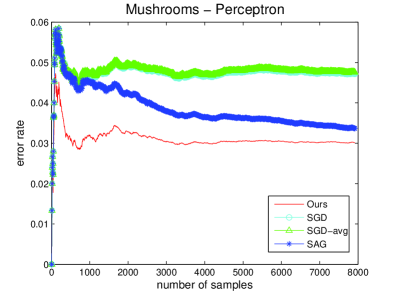
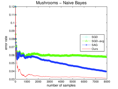
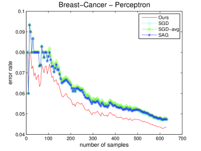
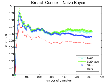
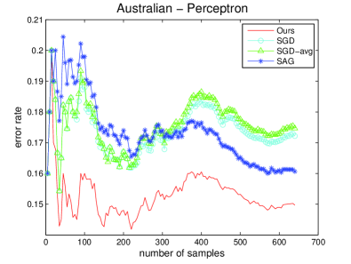
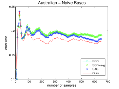
Figure 1: Plots of the error rate as online learning progresses for three benchmark datasets: Mushrooms, Breast-Cancer, and Australian. (Plots for other benchmarks datasets are provided in the supporting material.) The red curve in each graph shows the error rate for our method, as a function of the number samples processed in the online learning of ensemble weights. The cyan curves are results from SGD baseline, the green curves are results from the Polyak averaging baseline SGD-avg (Polyak and Juditsky, 1992), and the blue curves are results from the Stochastic Average Gradient baseline SAG (Schmidt et al., 2013).

Classification error rates for this experiment are shown in Tables 1 and 2. Our proposed method consistently performs the best for all datasets. Its superior performance against Voting is consistent with the asymptotic convergence analysis in Theorem 1. Its superior performance against the SGD baseline is consistent with the convergence rate analysis in Theorem 4. Polyak averaging (SGD-avg) does not improve the performance of basic SGD in general; this is consistent with the analysis in Xu (2011) which showed that, despite its optimal asymptotic convergence rate, a huge number of samples may be needed for Polyak averaging to reach its asymptotic region for a randomly chosen step size. SAG (Schmidt et al., 2013) is a close runner-up to our approach, but it has two limitations: 1) it requires knowing the length of the testing sequence a priori, and 2) as noted in Schmidt et al. (2013), the step size suggested in the theoretical analysis does not usually give the best result in practice, and thus the authors suggest a larger step size instead. In our experiments, we also found that the improvement of Schmidt et al. (2013) over the SGD baseline relies on tuning the step size to a value that is greater than that given in the theory. The performance of SAG reported here has taken advantage of these two points.

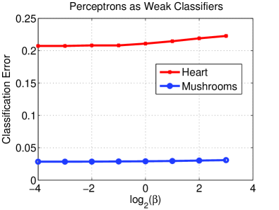
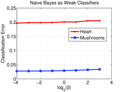
Figure 2: Experiments to evaluate different settings of $\beta$ for our online classifier ensemble method, using pre-trained Perceptrons and Naïve Bayes as weak classifiers. The mean error rate is computed over five random trials for the “Heart” and “Mushrooms” datasets. These results are consistent with all other benchmarks tested.

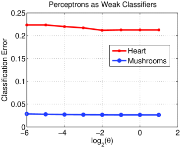
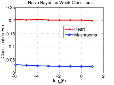
Figure 3: Experiments to evaluate different settings of $\theta$ for our online classifier ensemble method, using pre-trained Perceptrons and Naïve Bayes as weak classifiers. The mean error rate is computed over five random trials for the “Heart” and “Mushrooms” datasets. These results are consistent with all other benchmarks tested.

Fig. 1 shows plots of the convergence of online learning for three of the benchmark datasets. Plots for the other benchmark datasets are provided in the supplementary material. Each plot reports the classification error curves of our method, the SGD baseline, Polyak averaging SGD-avg (Polyak and Juditsky, 1992), and Stochastic Average Gradient SAG (Schmidt et al., 2013). Overall, for all methods, the error rate generally tends to decrease as the online learning process considers more and more samples. As is evident in the graphs, our method tends to attain lowest error rates overall, throughout each training sequence, for the compared methods for these benchmarks. Ideally, as an algorithm converges, the rate of cumulative error should tend to decrease as more samples are processed, approaching the minimal error rate that is achievable for the given set of pre-trained weak classifiers. Yet given the finite size of training sample set, and the randomness caused by different orderings of the sequences, we may not see the ideal monotonic curves. But in general, the trend of curves obtained by our method is consistent with the convergence analysis of Theorem 1. The online learning algorithm that converges faster should result in curves that go down more quickly in general. Again, given finite samples and different orderings, there is variance, but still, consistent with Theorem 2, the consistently better performance of our formulation vs. the compared methods is evident.

Fig 2 and Fig. 3 show plots for studying the sensitivity of parameter settings of our method. It is clear from the expression of the posterior mean (11) that the numerator containing $\alpha$ will be cancelled out in the prediction rule (12), therefore we just need to study the effect of $\beta$ and $\theta$. We select a short sequence, “Heart” and a long sequence, “Mushrooms” as two representative datasets. We plot the classification error rates of our method under different settings of $\beta$ (Fig. 2) and $\theta$ (Fig. 3), averaged over five random trials. It can be observed that the performance of our method is not very sensitive with respect to the changes in the settings of $\beta$ and $\theta$ even for a short sequence like “Heart” (270 samples). And the performance is more stable to the settings of these parameters for longer sequence like “Mushrooms” (8124 samples). This observation is consistent with the asymptotic property of our prediction rule (12). We observed similar behavior for all the other benchmark datasets we tested.

5.2 Comparison with Online Boosting Methods

We further compare our method with a single Perceptron/Naïve Bayes classifier that is updated online, and three representative online boosting methods reported in Chen et al. (2012): OzaBoost is the method proposed by Oza and Russell (2001), OGBoost is the online GradientBoost method proposed by Leistner et al. (2009), and OSBoost is the online Smooth-Boost method proposed by Chen et al. (2012). Ours-r is our proposed Bayesian ensemble method for online updated weak classifiers. All methods are trained and compared following the setup of Chen et al. (2012), where for each experimental trial, a set of 100 weak classifiers are initialized and updated online.

We use ten binary classification benchmark datasets that are also used by Chen et al. (2012). We discard the “Ijcnn1” and “Web Page” datasets from the tables of Chen et al. (2012), because they are highly biased with portions of positive samples around $0.09$ and $0.03$ respectively, and even a naïve “always negative” classifier attains comparably top performance.

Table 3: Experiments of online classifier ensemble using online Perceptrons as weak classifiers that are updated online. Mean error rate over five trials is shown in the table. We compare with a single online Perceptron classifier (Perceptron) and three representative online boosting methods reported in Chen et al. (2012). OzaBoost is the method proposed by Oza and Russell (2001), OGBoost is the online GradientBoost method proposed by Leistner et al. (2009), and OSBoost is the online Smooth-Boost method proposed by Chen et al. (2012). Our method (Ours-R) attains the top performance for most of the testing sequences.

dataset	# examples	Perceptron	OzaBoost	OGBoost	OSBoost	Ours-r
Heart	270	0.2489	0.2356	0.2267	0.2356	0.2134
Breast-Cancer	683	0.0592	0.0501	0.0445	0.0466	0.0419
Australian	693	0.2099	0.2012	0.1962	0.1872	0.1655
Diabetes	768	0.3216	0.3169	0.3313	0.3185	0.3098
German	1000	0.3256	0.3364	0.3142	0.3148	0.3105
Splice	3175	0.2717	0.2759	0.2625	0.2605	0.2584
Mushrooms	8124	0.0148	0.0080	0.0068	0.0060	0.0062
Adult	48842	0.2093	0.2045	0.2080	0.1994	0.1682
Cod-RNA	488565	0.2096	0.2170	0.2241	0.2075	0.1934
Covertype	581012	0.3437	0.3449	0.3482	0.3334	0.3115

Table 4: Experiments of online classifier ensemble using online Naïve Bayes as weak classifiers that are updated online. Mean error rate over five trials is shown in the table. We compare with a single online Naïve Bayes classifier (Naïve Bayes) and three representative online boosting methods reported in Chen et al. (2012). OzaBoost is the method proposed by Oza and Russell (2001), OGBoost is the online GradientBoost method proposed by Leistner et al. (2009), and OSBoost is the online Smooth-Boost method proposed by Chen et al. (2012). Our method (Ours-R) attains the top performance for 7 out of 10 testing sequences. For “Cod-RNA” our implementation of the Naïve Bayes baseline was unable to duplicate the reported result; ours gave 0.2555 instead.

dataset	# examples	Naive Bayes	OzaBoost	OGBoost	OSBoost	Ours-r
Heart	270	0.1904	0.2570	0.3037	0.2059	0.1755
Breast-Cancer	683	0.0474	0.0635	0.1004	0.0489	0.0408
Australian	693	0.1751	0.2133	0.2826	0.1849	0.1611
Diabetes	768	0.2664	0.3091	0.3292	0.2622	0.2467
German	1000	0.2988	0.3206	0.3598	0.2730	0.2667
Splice	3175	0.2520	0.1563	0.1863	0.1370	0.1344
Mushrooms	8124	0.0076	0.0049	0.0229	0.0029	0.0054
Adult	48842	0.2001	0.1912	0.1878	0.1581	0.1658
Cod-RNA	488565	0.2206$*$	0.0796	0.0568	0.0581	0.2552
Covertype	581012	0.3518	0.3293	0.3732	0.3634	0.3269

The error rates for this experiment are shown in Tables 3 and 4. As can be seen, our method outperforms competing methods using the Perceptron weak classifier in nearly all the benchmarks tested. Moreover, our method performs among the best for the Naïve Bayes weak classifier. It is worth noting that our method is the only one that outperforms the single classifier baseline in all benchmark datasets, which further confirms the effectiveness of the proposed ensemble scheme.

We also note that despite our best efforts to align both the weak classifier construction and experimental setup with competing methods (Chen et al., 2012; Chen, 2013), there are inevitably differences in weak classifier construction. Firstly, given that our method only focuses on optimizing the ensemble weights, each incoming sample is treated equally in the update of all weak classifiers, while all three online boosting methods adopt more sophisticated weighted update schemes for the weak classifiers, where the sample weight is dynamically adjusted during each round of update. Secondly, in order to make weak classifiers different from each other, our weak classifiers use only a subset of input features, while weak classifiers of competing methods use all features and are updated differently. As a result, the weak classifiers used by our method are actually weaker than in competing methods. Nevertheless, our method often compares favorably.

6 Additional Loss Functions for Online Ensemble Learning

We discuss other loss functions that fit into our Bayesian online ensemble learning framework. Note that the loss function (8) given in Section 4 is very simple, to the extent that the surrogate empirical loss (1) at each step can be directly minimized in closed-form. To demonstrate the flexibility of our framework, the empirical losses in the two examples we give below cannot be minimized directly, but they are still effectively solvable using our approach.

1. Consider the loss function

   $$\ell(\bm{\lambda};\mathbf{g}) = \sum\limits_{i=1}^{m}(1-\lambda_{i})\log g_{i}+\theta\sum\limits_{i=1}^{m}g_{i}$$ (19)

   $$+ \sum\limits_{i=1}^{m}\log\Gamma(\lambda_{i})-(\log\theta)\sum\limits_{i=1}^{m}\lambda_{i}$$

   where $\theta>0$ is a fixed parameter. The corresponding likelihood is given by the following product of Gamma distributions

   $$p(\mathbf{g}|\bm{\lambda})=\prod_{i=1}^{m}\frac{\theta^{\lambda_{i}}}{\Gamma(\lambda_{i})}g_{i}^{\lambda_{i}-1}e^{-\theta g_{i}}$$ (20)

   A conjugate prior for $\bm{\lambda}$ is available, in the form

   $$p(\bm{\lambda})\propto\prod_{i=1}^{m}\frac{a^{\lambda_{i}-1}\theta^{c\lambda_{i}}}{\Gamma(\lambda_{i})^{b}}$$

   where $a,b,c>0$ are hyperparameters. The posterior distribution of $\bm{\lambda}$ after $t$ steps is given by the Gamma distribution

   $$p(\bm{\lambda}|\mathbf{g}^{1:t})\propto\prod_{i=1}^{m}\frac{(a\prod\limits_{s=1}^{t}g_{i}^{s})^{\lambda_{i}-1}\theta^{(c+t)\lambda_{i}}}{\Gamma(\lambda_{i})^{(b+t)}}$$ (21)

   Note that given posterior (21), the posterior mean for each $\lambda_{i}$ is not available in closed-form, but it can be computed using standard numerical integration procedures, such as those provided in the Matlab Mathematics Toolbox (it only involves one-dimensional procedures because of the independence among the $\bm{\lambda}$). The corresponding prediction rule at each step is given by

   $$y=\left\{\begin{array}[]{rcl}1&\text{if}\ \sum\limits_{i=1}^{m}(1-\lambda_{i})\log\frac{g_{i}(\mathbf{x},1)}{g_{i}(\mathbf{x},-1)}+\theta\sum\limits_{i=1}^{m}(g_{i}(\mathbf{x},1)-g_{i}(\mathbf{x},-1))\leq 0\\ -1&\text{otherwise}\end{array}\right.\\$$

   Note that the likelihood function (20) of $g$ is a Gamma distribution, which has support $(0,\infty)$. For computational convenience, instead of choosing the ramp loss for $g$ as in Section 4, we can choose $g$ to be the logistic function.

2. We can extend the ensemble weights to include two correlated parameters for each weight, i.e., $\lambda_{i}=(\alpha_{i},\beta_{i})$. In this case, we may define the loss function as

   $$\ell(\bm{\alpha},\bm{\beta};\mathbf{g}) = \sum\limits_{i=1}^{m}\beta_{i}g_{i}+\sum\limits_{i=1}^{m}(1-\alpha_{i})\log g_{i}$$ (22)

   $$+ \sum\limits_{i=1}^{m}\log\Gamma(\alpha_{i})-\sum\limits_{i=1}^{m}\alpha_{i}\log\beta_{i}$$

   with the corresponding Gamma likelihood

   $$p(\mathbf{g}|\bm{\alpha},\bm{\beta})=\prod_{i=1}^{m}\frac{\beta_{i}^{\alpha_{i}}}{\Gamma(\alpha_{i})}g^{\alpha_{i}-1}e^{-\beta_{i}g_{i}}$$ (23)

   A conjugate prior is available for $\bm{\alpha}$ and $\bm{\beta}$ jointly

   $$p(\bm{\alpha},\bm{\beta})\propto\prod_{i=1}^{m}\frac{p^{\alpha_{i}-1}e^{-q\beta_{i}}}{\Gamma(\alpha_{i})^{r}\beta_{i}^{-\alpha_{i}s}}$$

   where $p,q,r,s$ are hyperparameters. The posterior distribution of $\bm{\alpha}$ and $\bm{\beta}$ after $t$ steps is given by the Gamma distribution

   $$p(\bm{\alpha},\bm{\beta}|\mathbf{g}^{1:t})\propto\prod_{i=1}^{m}\frac{(p\prod\limits_{s=1}^{t}g_{i}^{s})^{\alpha_{i}-1}e^{-(q+\sum_{s=1}^{t}g_{i}^{s})\beta_{i}}}{\Gamma(\alpha_{i})^{(r+t)}\beta_{i}^{-\alpha_{i}(s+t)}}$$ (24)

   Again, the posterior mean for (24) is not available in closed-form and we can approximate it using numerical methods. The corresponding prediction rule at each step is given by

   $$y=\left\{\begin{array}[]{rcl}1&\mbox{if}\ \sum\limits_{i=1}^{m}(1-\alpha_{i})\log\frac{g_{i}(\mathbf{x},1)}{g_{i}(\mathbf{x},-1)}+\sum\limits_{i=1}^{m}\beta_{i}(g_{i}(\mathbf{x},1)-g_{i}(\mathbf{x},-1))\leq 0\\ -1&\mbox{otherwise}\end{array}\right.\\$$

Note that both of these two loss functions satisfy Assumption 1. Similar as the example proposed in Section 4, the Hessian of $L_{T}$ turns out to not depend on $g^{1:T}$, therefore all conditions of Assumption 1 can be verified easily. As a result, applying Algorithm 1 on these two loss functions for solving the online ensemble learning problem also possesses the convergence properties given by Theorems 1 and 2.

We follow the experimental setup of Section 5.1 to compare our proposed loss (8) with the additional losses (19) and (22) discussed here, using pre-trained Perceptron and Naïve Bayes as weak classifiers. The loss function $g$ for weak classifier $c$ is chosen as a logistic function of $y\cdot c(x)$. According to the posterior update rules given in (21) and (24), hyper parameters $b,c$ and $r,s$ will keep increasing as online learning proceeds. However, we observe in practice that the numerical integration of posterior means based on posterior distributions (21) and (24) will not converge if the values of hyper parameters $b,c,r,s$ are too large. In our experiments, we set upper bounds for these parameters. In particular, we set the upper bound for $b$ and $c$ as $1000$, the upper bound for $r$ and $s$ as $200.5$ and $200$ respectively (Since $s$ should be strictly less than $r$, we use the following initialization: $s=1$, $r=1.5$, as suggested by Fink, 1997).

Averaged classification error rate over five trials for this experiment is shown in Table 5. Note that the result in this table should not be directly compared with those reported in Tables 1 and 2, given the loss function $g$ for weak classifiers is chosen differently. We observe that loss (22) works slightly better than loss (19), which is reasonable given more parameters in the formula of (22). This advantage also leads to a superior performance to loss (8) proposed in Section 4 for shorter sequences, such as “Heart”, “Ionosphere” and “Sonar”. However, for longer sequences, loss (8) still has some advantage because of the closed-form posterior mean.

Table 5: Experiments of online classifier ensemble using pre-trained Perceptrons/Naïve Bayes as weak classifiers and keeping them fixed online. Mean error rate over five random trials is shown in the table. We compare our method using the proposed loss function (8) with alternative losses defined by (19) and (22). In general, the loss function (8) that enables closed-form posterior mean performs the best.

		Perceptron weak learner			Naïve Bayes weak learner
dataset	# examples	loss (8)	loss (19)	loss (22)	loss (8)	loss (19)	loss (22)
Heart	270	0.203	0.208	0.198	0.197	0.204	0.196
Breast-Cancer	683	0.065	0.070	0.068	0.045	0.050	0.046
Australian	693	0.183	0.207	0.200	0.191	0.209	0.203
Diabetes	768	0.301	0.307	0.300	0.285	0.287	0.284
German	1000	0.338	0.347	0.348	0.292	0.292	0.293
Splice	3175	0.390	0.418	0.418	0.144	0.150	0.150
Mushrooms	8124	0.028	0.032	0.031	0.025	0.047	0.046
Ionosphere	351	0.293	0.295	0.259	0.171	0.172	0.171
Sonar	208	0.385	0.391	0.380	0.301	0.302	0.303
SVMguide3	1284	0.265	0.278	0.276	0.222	0.226	0.225

7 Conclusion

We proposed a Bayesian approach for online estimation of the weights of a classifier ensemble. This approach was based on an empirical risk minimization property of the posterior distribution, and involved suitably choosing the likelihood function based on a user-defined choice of loss function. We developed the theoretical foundation, and identified the class of loss functions, for which the update sequence generated by our approach converged to the stationary risk minimizer. We demonstrated that, unlike standard SGD, the convergence guarantee was global and that the rate was optimal in a well-defined asymptotic sense. Moreover, experiments on real-world datasets demonstrated that our approach compared favorably to state-of-the-art SGD methods and online boosting methods. In future work, we will study further generalization of the scope of loss functions, and the extension of our framework to non-stationary environments.

References

- Asmussen and Glynn (2007) S. Asmussen and P. W. Glynn. Stochastic simulation: Algorithms and analysis. Springer, 2007.
- Babenko et al. (2009a) B. Babenko, M. H. Yang, and S. Belongie. Visual tracking with online multiple instance learning. In Proc. IEEE Conf. on Computer Vision and Pattern Recognition (CVPR), pages 983–990, 2009a.
- Babenko et al. (2009b) B. Babenko, M. H. Yang, and S. Belongie. A family of online boosting algorithms. In ICCV Workshops, pages 1346–1353, 2009b.
- Bai et al. (2014) Qinxun Bai, Henry Lam, and Stan Sclaroff. A bayesian framework for online classifier ensemble. In Proc. International Conf. on Machine Learning (ICML), 2014.
- Cesa-Bianchi and Lugosi (2003) N. Cesa-Bianchi and G. Lugosi. Potential-based algorithms in on-line prediction and game theory. Machine Learning, pages 239–261, 2003.
- Chen (1985) C. F. Chen. On asymptotic normality of limiting density functions with bayesian implications. Journal of the Royal Statistical Society, pages 540–546, 1985.
- Chen (2013) S. T. Chen. personal communication, 2013.
- Chen et al. (2012) S. T. Chen, H. T. Lin, and C. J. Lu. An online boosting algorithm with theoretical justifications. In Proc. International Conf. on Machine Learning (ICML), pages 1007–1014, 2012.
- Durrett (2010) R. Durrett. Probability Theory and Examples. Cambridge Series in Statistical and Probabilistic Mathematics, 4th edition, 2010.
- Fink (1997) Daniel Fink. A compendium of conjugate priors. 1997.
- Freund and Schapire (1995) Y. Freund and R. E. Schapire. A desicion-theoretic generalization of on-line learning and an application to boosting. In Computational learning theory, pages 23–37, 1995.
- Friedman (2001) J. H. Friedman. Greedy function approximation: a gradient boosting machine. Annals of Statistics, pages 1189–1232, 2001.
- Grabner and Bischof (2006) H. Grabner and H. Bischof. On-line boosting and vision. In Proc. IEEE Conf. on Computer Vision and Pattern Recognition (CVPR), pages 260–267, 2006.
- Grabner et al. (2008) H. Grabner, C. Leistner, and H. Bischof. Semi-supervised on-line boosting for robust tracking. In Proc. European Conf. on Computer Vision (ECCV), pages 234–247. 2008.
- Grbovic and Vucetic (2011) M. Grbovic and S. Vucetic. Tracking concept change with incremental boosting by minimization of the evolving exponential loss. In Machine Learning and Knowledge Discovery in Databases, pages 516–532. 2011.
- Hardy et al. (1952) G. H. Hardy, J. E. Littlewood, and G. Pólya. Inequalities. Cambridge university press, 1952.
- Hoeting et al. (1999) J. A. Hoeting, D. Madigan, A. E. Raftery, and C. T. Volinsky. Bayesian model averaging: a tutorial. Statistical science, pages 382–401, 1999.
- Hu et al. (2007) Jiaqiao Hu, Michael C Fu, and Steven I Marcus. A model reference adaptive search method for global optimization. Operations Research, 55(3):549–568, 2007.
- Kolter and Maloof (2007) J. Z. Kolter and M. A. Maloof. Dynamic weighted majority: An ensemble method for drifting concepts. Journal of Machine Learning Research, pages 2755–2790, 2007.
- Kolter and Maloof (2005) J.Z. Kolter and M.A. Maloof. Using additive expert ensembles to cope with concept drift. In Proc. International Conf. on Machine Learning (ICML), pages 449–456, 2005.
- Kushner and Yin (2003) H. J. Kushner and G. Yin. Stochastic approximation and recursive algorithms and applications. Springer, 2003.
- Leistner et al. (2009) C. Leistner, A. Saffari, P. M Roth, and H. Bischof. On robustness of on-line boosting-a competitive study. In ICCV Workshops, pages 1362–1369, 2009.
- Liu and Yu (2007) X. Liu and T. Yu. Gradient feature selection for online boosting. In Proc. IEEE International Conf. on Computer Vision (ICCV), pages 1–8, 2007.
- MacKay (2003) David JC MacKay. Information theory, inference and learning algorithms. Cambridge university press, 2003.
- Mason et al. (1999) L. Mason, J. Baxter, P. Bartlett, and M. Frean. Boosting algorithms as gradient descent in function space. In NIPS, 1999.
- Minku (2011) L.L. Minku. Online ensemble learning in the presence of concept drift. PhD thesis, University of Birmingham, 2011.
- Oza (2001) N. C. Oza. Online ensemble learning. PhD thesis, University of California, Berkeley, 2001.
- Oza and Russell (2001) N. C. Oza and S. Russell. Online bagging and boosting. In AISTATS, pages 105–112, 2001.
- Pasupathy and Kim (2011) R. Pasupathy and S. Kim. The stochastic root-finding problem: overview, solutions, and open questions. ACM Trans. on Modeling and Computer Simulation, 21(3):19, 2011.
- Pelossof et al. (2009) R. Pelossof, M. Jones, I. Vovsha, and C. Rudin. Online coordinate boosting. In ICCV Workshops, pages 1354–1361, 2009.
- Polyak and Juditsky (1992) Boris T Polyak and Anatoli B Juditsky. Acceleration of stochastic approximation by averaging. SIAM Journal on Control and Optimization, 30(4):838–855, 1992.
- Rubinstein and Kroese (2004) Reuven Y Rubinstein and Dirk P Kroese. The cross-entropy method: a unified approach to combinatorial optimization, Monte-Carlo simulation and machine learning. Springer, 2004.
- Saffari et al. (2010) A. Saffari, M. Godec, T. Pock, C. Leistner, and H. Bischof. Online multi-class lpboost. In Proc. IEEE Conf. on Computer Vision and Pattern Recognition (CVPR), pages 3570–3577, 2010.
- Schapire (2001) Robert E Schapire. Drifting games. Machine Learning, pages 265–291, 2001.
- Schmidt et al. (2013) Mark Schmidt, Nicolas Le Roux, and Francis Bach. Minimizing finite sums with the stochastic average gradient. arXiv preprint arXiv:1309.2388, 2013.
- Serfling (2009) R. J. Serfling. Approximation theorems of mathematical statistics. Wiley. com, 2009.
- Telgarsky (2012) M. Telgarsky. A primal-dual convergence analysis of boosting. Journal of Machine Learning Research, pages 561–606, 2012.
- Wang et al. (2003) H. Wang, W. Fan, P.S. Yu, and J. Han. Mining concept-drifting data streams using ensemble classifiers. In Proc. ACM SIGKDD Conf. on Knowledge Discovery and Data Mining (KDD), pages 226–235, 2003.
- Xu (2011) Wei Xu. Towards optimal one pass large scale learning with averaged stochastic gradient descent. arXiv preprint arXiv:1107.2490, 2011.
- Zlochin et al. (2004) Mark Zlochin, Mauro Birattari, Nicolas Meuleau, and Marco Dorigo. Model-based search for combinatorial optimization: A critical survey. Annals of Operations Research, 131(1-4):373–395, 2004.