The Ising Spin Glass in dimension four

Abstract

The critical behaviors of the bimodal and Gaussian Ising spin glass (ISG) models in dimension four are studied through extensive numerical simulations, and from an analysis of high temperature series expansion (HTSE) data of Klein et al. (1991). The simulations include standard finite size scaling measurements, thermodynamic limit regime measurements, and analyses which provide estimates of critical exponents without any consideration of the critical temperature. The higher order HTSE series for the bimodal model provide accurate estimates of the critical temperature and critical exponents. These estimates are independent of and fully consistent with the simulation values. Comparisons between ISG models in dimension four show that the critical exponents and the critical constants for dimensionless observables depend on the form of the interaction distribution of the model.

I Introduction

Renormalization Group Theory (RGT) for thermodynamic phase transitions wilson:75 and the Edwards-Anderson model for Ising Spin Glasses (ISGs) edwards:75 were introduced almost simultaneously forty years ago. Ever since it has been tacitly assumed as self-evident that the standard RGT universality rules should apply to ISGs. As far as we know there is no rigorous theoretical proof that this ISG hypothesis holds, though confirmations have been reported a number of times based on numerical data bhatt:88 ; katzgraber:06 ; hasenbusch:08 ; jorg:08 . The universality principle states that for all systems within a universality class the critical exponents are strictly identical and do not depend on the microscopic parameters of the model. All ISG models in a given dimension are supposed to be in the same universality class, on the assumption that the form of the interaction distribution is an irrelevant microscopic parameter.

Thus in the family of simple ferromagnets, within a universality class of models having space dimension $d$ and spin dimensionality $n$, all models have identical critical properties corresponding to an isolated fixed point in the renormalisation group flow. However, diluted ferromagnets of given $d,n$ have a different (dilution independent) set of critical exponents, with values which correspond to a separate isolated fixed point ballesteros:98 ; calabrese:03 . For a few special cases of spin models in dimension two (discussed for instance in Ref. cardy:87 ) the critical behavior is more complicated and corresponds to a line of fixed points rather than an isolated fixed point; critical parameters vary continuously according to motion along the line, produced by a marginal operator. From the empirical ISG data below there appear for the moment to be two possible scenarios : two classes of ISGs (such as models with continuous distributions and those with discrete distributions) or alternatively ISG exponents which vary continuously with a parameter such as the kurtosis of the interaction distribution. In any case it has been stated by authoritative authors that “classical tools of RGT analysis are not suitable for spin glasses” parisi:01 ; castellana:11 ; angelini:13 although no explicit theoretical predictions have been made so far concerning the important question of universality.

Here we combine numerical simulation and high temperature series expansion (HTSE) data on the bimodal and Gaussian ISGs in dimension four so as to obtain accurate and reliable values for the critical parameters in this model. We discuss a number of different methods for exploiting numerical data, and show that for each model these are consistent. Comparisons between these and other estimates on ISG models in the same dimension but with different interaction distributions show that the critical exponents and the critical constants for dimensionless parameters depend on the form of the interaction distribution.

II Numerical techniques

The Hamiltonian is as usual

$$\mathcal{H}=-\sum_{ij}J_{ij}S_{i}S_{j}$$ (1)

with the near neighbor symmetric distributions normalized to $\langle J_{ij}^{2}\rangle=1$. The Ising spins live on simple hyper-cubic lattices with periodic boundary conditions. We have studied the bimodal model with a $\pm J$ interaction distribution and the Gaussian interaction distribution model. We will compare with published measurements on these and other $4$d ISGs. We will use the inverse temperature $\beta=\langle J_{ij}^{2}\rangle^{1/2}/T=1/T$, with the normalization above, or alternatively $w=\tanh^{2}(\beta)$, to signify the temperature. The spin overlap parameter is defined by

$$q=\frac{1}{N}\left\langle\sum_{i}S_{i}^{A}S_{i}^{B}\right\rangle$$ (2)

where $A$ and $B$ indicate two copies of the same system and $N$ is the number of sites.

The simulations were carried out using the exchange Monte Carlo method for equilibration using so called multi-spin coding, on $2^{14}$ (up to $L=7$) or $2^{13}$ (for larger $L$) individual samples at each size. An exchange was attempted after every sweep with a success rate of at least 30%. At least 40 temperatures were used forming a geometric progression reaching down to $\beta_{\max}=0.55$ for the bimodal model and $\beta_{\max}=0.60$ for the Gaussian model. This ensures that our data span the critical temperature region which is essential for the FSS fits. Near the critical temperature the $\beta$ step length was at most $0.03$. The various systems were deemed to have reached equilibrium when the sample average susceptibility for the lowest temperature showed no trend between runs. For example, for $L=12$ this means about $200000$ sweep-exchange steps.

After equilibration, at least $200000$ measurements were made for each sample for all sizes, taking place after every sweep-exchange step. Data were registered for the energy $E(\beta,L)$, the correlation length $\xi(\beta,L)$, and for the spin overlap moments. In addition the correlations $\langle E(\beta,L),U(\beta,L)\rangle$ between the energy and observables $U(\beta,L)$ were also registered so that thermodynamic derivatives could be evaluated using the relation $\partial U(\beta,L)/\partial\beta=\langle U(\beta,L)\,E(\beta,L)\rangle-\langle U(\beta,L)\rangle\langle E(\beta,L)\rangle$ where $E(\beta,L)$ is the energy ferrenberg:91 . Bootstrap analyses of the errors in the derivatives as well as in the observables $U(\beta,L)$ themselves were carried out.

III Finite size scaling

Figure 1: (Color online) The $4$d bimodal ISG. FSS for the correlation length ratio $\xi(\beta,L)/L$ at fixed inverse temperatures $\beta=0.5100$, $0.5075$, $0.5050$, $0.5025$, $0.5000$,$0.4975$ from top to bottom, against $1/L^{1.2}$. Red squares : present data, black circles : read from Ref. banos:12 . Dashed line : critical behavior.

Figure 2: (Color online) The $4$d bimodal ISG. FSS for the Binder cumulant $g(\beta,L)$ at fixed inverse temperatures $\beta=0.5100$, $0.5075$, $0.5050$, $0.5025$, $0.5000$, $0.4975$ from top to bottom, against $1/L^{1.2}$. Red squares : present data, black circles : read from Ref. banos:12 . Dashed line : critical behavior.

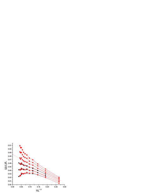
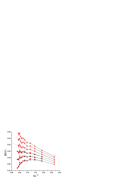
ISG simulations are much more demanding numerically than are those on, say, pure ferromagnet transitions with no interaction disorder. The traditional approach to criticality in ISGs has been to study the temperature and size dependence of dimensionless observables, principally the Binder cumulant $g(\beta,L)$ and the correlation length ratio $\xi(\beta,L)/L$, in the near-transition region and to estimate the critical temperature and exponents through finite size scaling (FSS) relations after taking means over large numbers of samples. Finite size corrections to scaling must be allowed for explicitly which can be delicate as the range of sizes $L$ is generally small. On this FSS approach the estimated values for the critical exponents are very sensitive to the critical inverse temperature $\beta_{c}$ estimates. Here we first obtain estimates for $\beta_{c}$ and the critical parameters using FSS.

The data for standard dimensionless observables, the Binder cumulant

$$g(\beta,L)=\frac{1}{2}\left(3-\frac{[\langle q^{4}\rangle]}{[\langle q^{2}\rangle]^{2}}\right)$$ (3)

and the correlation length ratio $\xi(\beta,L)/L$ are shown in Figs. 1 and 2 as functions of size at fixed temperatures near $\beta_{c}$. We show data from the present simulations together with data taken from the appropriate figures in Ref. banos:12 . The standard FSS expression for a dimensionless observable $U=U(\beta,L)$, valid in the critical region is

$$U=U_{c}+AL^{-\omega}+B(\beta-\beta_{c})L^{1/\nu}\left(1+CL^{-\omega}+\cdots\right)$$ (4)

where $U_{c}=U(\beta_{c},\infty)$. We plot $g(\beta,L)$ and $\xi(\beta,L)/L$ against $1/L^{\omega}$ with $\omega=1.2$. The choice of this value, close to the estimate $\omega=1.04(10)$ of Ref. banos:12 , will be explained below. By inspection there is good point by point consistency between the present data and those of Ref. banos:12 where the statistical accuracy was much higher, but where the temperatures studied did not quite span the critical temperature. The consistency between the two data sets implies that full equilibrium has been reached. The data in Figs. 1 and 2 for fixed $\beta$ should tend to straight lines at criticality, curving upwards and downwards respectively at large $L$ for $\beta$ higher and lower than $\beta_{c}$; one can estimate $\beta_{c}=0.505(1)$ from this criterion. The value is marginally higher than the estimate $\beta_{c}=0.5023(6)$ of Ref. banos:12 . Data we have obtained on other dimensionless parameters lead to very similar estimates for $\beta_{c}$ lundow:14 .

It is important to consider the value of the irrelevant scaling field thermal correction exponent $\theta$ or equivalently the finite size correction exponent $\omega=\theta/\nu$. The first term in the RGT $\epsilon$-expansion for the ISG leading irrelevant operator is $\theta(d)=(6-d)$ dedominicis ; bray , so $\theta(3)\approx 3$, $\theta(4)\approx 2$, $\theta(5)\approx 1$ (see ballesteros:97 for the analogous site percolation $\epsilon$-expansion). These values are only indicative as they are obtained from the leading terms of a series which (like the ${\epsilon}$-expansion series for the other exponents in ISGs) has never been summed. However, the values are qualitatively consistent with the observed $\theta(d)$ and $\omega(d)=\theta(d)/\nu(d)$ values for $d=3$, $4$ and $5$. FSS estimates in $3$d are $\omega=1.12(10)$ and $\nu=2.56(4)$ baity:13 so $\theta(3)=\omega\nu\approx 3$. HTSE estimates for various ISG models in $4$d are $\theta(4)\approx 1.5$ and in $5$d, $\theta(5)\approx 1.0$ daboul:04 ; klein:91 . Simulation estimates in $4$d and $5$d are consistent with these values banos:12 ; lundow:14 ; lundow . Potentially there can also be an analytic correction with exponent ballesteros:99 $\omega_{a}\approx\gamma/\nu>2$ in $4$d. If an analytic contribution is indeed present in $4$d in addition to the leading conformal correction, the effective exponent of the combined correction will be slightly increased.

The relative strengths of the leading conformal correction and the analytic correction will depend on the observable so the effective exponent for the combination can be expected to vary somewhat from observable to observable within a narrow range of values.

The leading irrelevant scaling field correction is by definition the correction of this type which has the smallest exponent $\theta$. From the overall agreement between the $\epsilon$-expansion and observed values, one can be fully confident that the leading irrelevant operator correction in $4$d is $\omega(4)\approx 1.5$, and hence no hypothetical correction term with a much smaller exponent (which if it existed would modify the behavior at very large $L$) can exist. Extrapolations of observed FSS data to infinite $L$ using a correction exponent $\omega\approx 1.3$ are valid, which justifies the natural straight line extrapolations at $\beta_{c}$ in Figs. 1 and 2. Similarly valid fits to the ThL data in Figs. 6 and 7 are made with a leading correction term having an exponent $\theta\approx 1.5$. No hypothetical small exponent correction term producing ”reentrant” behavior exists.

For each dimensionless observable $U(\beta,L)$, extrapolation to infinite $L$ at $\beta_{c}$ gives an estimate for a critical parameter $U(\beta_{c},\infty)$ characteristic of the universality class. For the bimodal ISG in dimension four these data show $g(\beta_{c},\infty)=0.525(5)$ and $(\xi/L)(\beta_{c},\infty)=0.485(5)$.

With the FSS rule Eq. (4) for a dimensionless observable $U(\beta,L)$ the critical exponent $\nu$ can be estimated in principle from $[dU(\beta,L)/d\beta)]_{\beta_{c}}=BL^{1/\nu}$. To obtain these $\nu$ estimates, the fits are multi-parameter as they involve simultaneous estimates for $\beta_{c}$, $\omega$, and the parameters $A$, $B$ and $C$ as well as $\nu$. Nevertheless in practice reasonably precise values for $\nu$ can be obtained. From analyses of data sets such as those shown in Figs. 1 and 2 on a number of different dimensionless observables, a global estimate for the bimodal model is $\nu=1.13(1)$ lundow:14 .

IV Thermodynamic derivative peak analysis

Figure 3: (Color online) The $4$d bimodal ISG. Thermodynamic derivative peak $D_{\max}=[\partial U(\beta,L)/\partial\beta]_{\max}$ data for dimensionless observables $U=W_{q},h,g$ (black squares, blue circles, red triangles). The peak location $\beta_{\max}(L)$ against the inverse peak height $1/D_{\max}(L)$.

Figure 4: (Color online) The $4$d bimodal ISG. The Binder cumulant derivative peak height maximum $[\partial g(\beta,L)/\partial\beta]_{\max}$ normalized by $L$, against $L$ (log-log scaling).

Figure 5: (Color online) The $4$d bimodal ISG. The effective susceptibility exponent $\gamma(\tau,L)$ with $\beta_{c}=0.505$. Sizes $L=14$ to $5$ from left to right. The red continuous curve is calculated from the tabulated HTSE terms in Ref. daboul:04 . The green continuous curve is an overall fit.

Figure 6: (Color online) The $4$d bimodal ISG. The effective correlation length exponent $\nu(\tau,L)$ with $\beta_{c}=0.505$. Sizes $L=14$ to $4$ from left to right. The green continuous curve is an overall fit. The red arrow is the exact bimodal high temperature limit $\nu(\tau=1)=(d-1/3)\beta_{c}^{2}$.

Figure 7: (Color online) The $4$d bimodal ISG. The ratio $\chi(\beta,L)/(\xi(\beta,L)/\beta)^{2}$ as function of $\xi(\beta,L)/\beta$ (log-log scaling). Sizes $L=6,8,10,12,14$ from left to right. The green continuous curve is an overall fit.

Near criticality in a ferromagnet for dimensionless observables $U(\beta,L)$ the heights of the peaks $D_{\max}(U,L)$ of the thermodynamic derivatives $D(U,L)=\partial U(\beta,L)/\partial\beta$ scale for large $L$ as ferrenberg:91 ; weigel:09

$$[\partial U(\beta,L)/\partial\beta]_{\max}\propto L^{1/\nu}\left(1+aL^{-\omega/\nu}+\cdots\right)$$ (5)

The temperature location of the derivative peak $\beta_{\max}(U,L)$ similarly scales as

$$\beta_{c}-\beta_{\max}(U,L)\propto L^{-1/\nu}(1+bL^{-\omega/\nu}+\cdots)$$ (6)

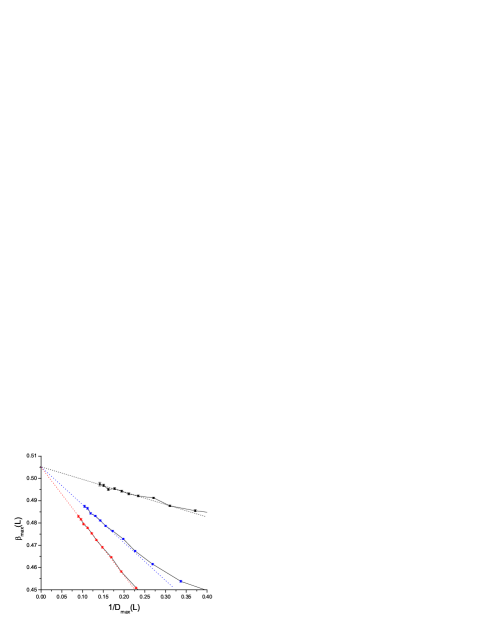
As both $\beta_{c}-\beta_{\max}(U,L)$ and $1/D_{\max}(U,L)$ vary as $L^{-1/\nu}$ at large $L$, a plot of the peak locations against the inverse peak heights tends linearly to $\beta_{c}$ at large $L$. These estimates of $\beta_{c}$ are independent of the FSS estimates. The observables used for $U(\beta,L)$ ferrenberg:91 can be for instance the Binder cumulant $g(\beta,L)$ or the logarithm of the finite size susceptibility $\ln(\chi(\beta,L))$.

For an ISG just the same thermodynamic differential peak methodology can be used as in the ferromagnet. As far as we are aware this analysis has not been used previously in the ISG context. In Fig. 3 we show data for peak height locations $\beta_{\max}(U,L)$ against the inverse peak height $1/D_{\max}(U,L)$ for the derivatives $\partial U(\beta,L)/\partial\beta$ with dimensionless observables $U(\beta,L)$, the Binder cumulant $g(\beta,L)$, together with $W_{q}(\beta,L)$ and $h(\beta,L)$ defined by

$$W_{q}(\beta,L)=\frac{1}{\pi-2}\left(\pi\frac{[\langle|q|\rangle]^{2}}{[\langle q^{2}\rangle]}-2\right)$$ (7)

and

$$h(\beta,L)=\frac{1}{\sqrt{\pi}-\sqrt{8}}\left(\sqrt{\pi}\frac{[\langle|q^{3}|\rangle]}{[\langle q^{2}\rangle]^{3/2}}-\sqrt{8}\right)$$ (8)

where the coefficients have been chosen so that the parameters go from 0 at high temperature to 1 at low temperature. In Fig. 3 the linear extrapolations of the three sets of data points lead consistently to $\beta_{c}=0.505(1)$, in full agreement with the FSS data.

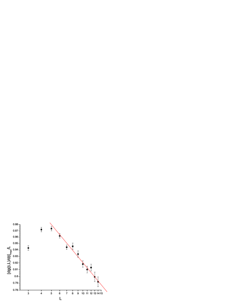
From the thermodynamic derivatives, ”The critical exponent $\nu$ can be estimated without any consideration of the critical coupling $\beta_{c}$” ferrenberg:91 . As the exponent $\nu$ is close to $1$ in $4$d, we choose to plot data for the normalised Binder cumulant derivative $\ln(D_{\max}(L)/L)$ against $\ln(L)$, Fig. 4. Corrections to scaling are visible for small $L$, but for $L>4$ the slope is $-0.0890(5)$, which corresponds to $\nu=1.13(1)$, in full agreement with the FSS estimate above.

V Thermodynamic limit derivatives

Analyses using the standard RGT scaling variable $t=1-T/T_{c}=1-\beta_{c}/\beta$, either in ferromagnets or in spin glasses, are restricted to the critical region and the FSS regime $L\ll\xi(\beta,\infty)$, because $t$ tends to diverge at high temperatures so scaling corrections automatically proliferate outside the critical regime. This is unnecessary. A natural scaling variable, which has been used for the scaling of the susceptibility in ferromagnets for more than 50 years, is $\tau=1-\beta/\beta_{c}$ fisher:67 ; wegner:72 ; gartenhaus:88 ; butera:02 . The Wegner thermodynamic limit (ThL) susceptibility scaling expression wegner:72 , which is expressed in terms of $\tau$ and is valid from criticality to infinite temperature,is

$$\chi(\tau,\infty)=C_{\chi}\tau^{-\gamma}\left(1+a_{\chi}\tau^{\theta}+b_{\chi}\tau+\cdots\right)$$ (9)

At criticality $\tau$ becomes identical to $t$ and tends to $1$ at infinite temperature, so the corrections in the Wegner expression are well behaved for the entire paramagnetic temperature range. The first correction term in the equation is the leading confluent correction and the second an analytic correction. There is a closure condition as $\chi(\tau=1)\equiv 1$. In ISGs as the interaction energy is $\langle J^{2}\rangle$, not $\langle J\rangle$, and the appropriate scaling variable is $\tau=1-(\beta/\beta_{c})^{2}$ or $\tau_{w}=1-(\tanh(\beta)/\tanh(\beta_{c}))^{2}$. This is the scaling variable which was used from the beginning in ISG HTSE work fisch:77 ; singh:86 ; klein:91 ; daboul:04 ; campbell:06 but curiously not in most analyses of numerical simulations. The Wegner expression for the susceptibility wegner:72 carries over, with the appropriate definition for $\tau$.

It has been pointed out that in Ising ferromagnets the ThL expression for the second moment correlation length $\xi(\tau)$ analogous to the Wegner expression for the susceptibility is campbell:06 ; campbell:08 ; butera:02 ; lundow

$$\xi(\tau)=C_{\xi}\beta^{1/2}\tau^{-\nu}\left(1+a_{\xi}\tau^{\theta}+\cdots\right)$$ (10)

The factor $\beta^{1/2}$ arises because the generic infinite temperature limit behavior is $\xi(\tau)/\beta^{1/2}\to 1$.

In ISGs the factor $\beta^{1/2}$ becomes $\beta$, again because $\langle J^{2}\rangle$ replaces $\langle J\rangle$ campbell:06 , so

$$\xi(\tau)=C_{\xi}\beta\tau^{-\nu}\left(1+a_{\xi}\tau^{\theta}+\cdots\right)$$ (11)

with the ISG $\tau$. Following a well-established protocol kouvel:64 ; butera:02 one can define a temperature dependent effective exponent for the susceptibility

$$\gamma(\tau)=-\partial\ln(\chi(\tau))/\partial\ln(\tau)$$ (12)

and for the second moment correlation length

$$\nu(\tau)=-\partial\ln(\xi(\tau)/\beta)/\partial\ln(\tau)$$ (13)

which tend to the critical $\gamma$ and $\nu$ respectively at criticality, and to $2d\beta_{c}^{2}$ and $(d-K/3)\beta_{c}^{2}$ respectively in the high temperature $\tau=1$ limit, where $K$ is the kurtosis of the interaction distribution. ($K=1$ in the bimodal case and $K=3$ for the Gaussian).

For data in the ThL regime, the Wegner expression with two correction terms Eq. (9) translates exactly into

$$\gamma(\tau)=\gamma-\frac{a_{\chi}\theta\tau^{\theta}+b_{\chi}y\tau^{y}}{1+a_{\chi}\tau^{\theta}+b_{\chi}\tau^{y}}$$ (14)

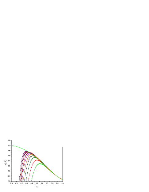
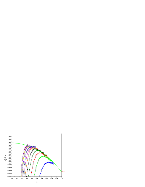
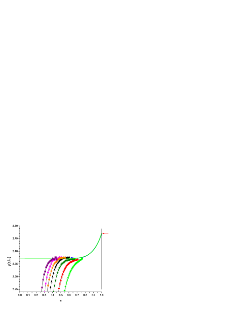
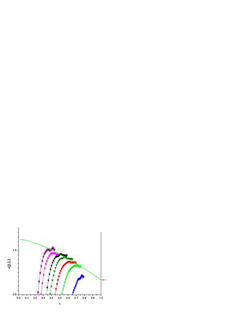
where the second term is an effective subleading correction. There is an equivalent relation for $\nu(\tau)$. Fixing $\beta_{c}=0.505$, the $\gamma(\tau)$ and $\nu(\tau)$ plots for all the different sizes $L$ are shown in Fig. 5 and Fig. 6. In Fig. 5 the effective $\gamma(\beta)$ evaluated from an explicit sum of the first 15 terms in the HTSE series of Ref. daboul:04 is also shown.

The fit curves are adjusted to those data which are in the ThL regime, and the fit is then extrapolated to criticality to obtain estimates for the critical $\gamma$ and $\nu$. Just as for $\omega$ in the FSS regime, $\theta$ is the lowest correction exponent and so a further hypothetical correction term with a much lower exponent which could modify the form of the fit curve between the ThL data and criticality can be ruled out. The $\gamma(\tau)$ and $\nu(\tau)$ plots are however rather sensitive to the exact value of $\beta_{c}$.

The fits shown correspond to an ISG temperature dependent susceptibility effectively fitted by

$$\chi(\beta)=0.634\tau^{-2.70}\left(1+0.38\tau^{1.5}+0.22\tau^{3}-0.022\tau^{8}\right)$$ (15)

and a second moment correlation length

$$\xi(\beta)=0.914\beta\tau^{-1.12}\left(1+0.055\tau^{1.5}+0.042\tau^{3}\right)$$ (16)

so with estimated critical exponents $\gamma=2.70$, $\nu=1.12$, $\theta=1.5$, with a leading correction term and further higher order terms.

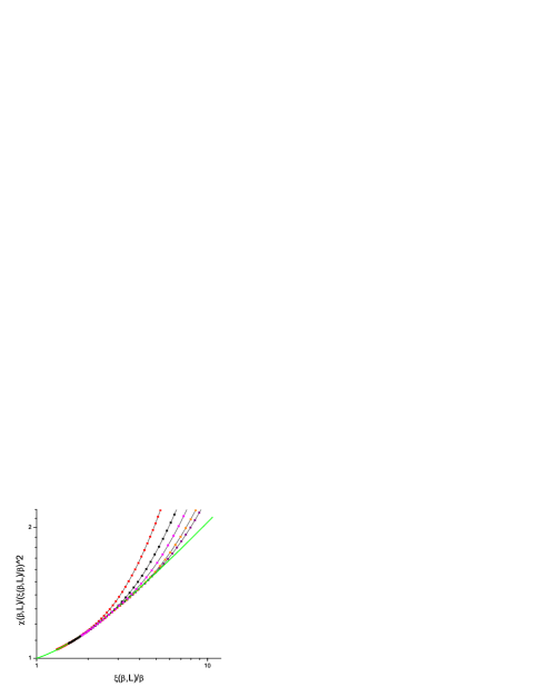
The ratio

$$\frac{\gamma(\tau,L)}{\nu(\tau,L)}=\frac{\partial\ln\chi(\beta^{2},L)/\partial\ln\tau}{\partial\ln(\xi(\beta^{2},L)/\beta)/\partial\ln\tau}=2-\eta(\beta,L)$$ (17)

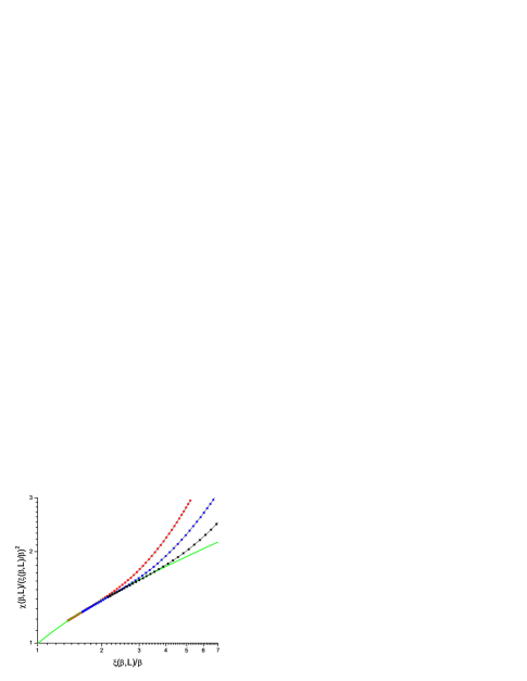
does not involve $\beta_{c}$, so $\eta(\beta,L)$ can be measured without any knowledge of $\beta_{c}$. Then the $\eta(\beta,L)$ as functions of $\beta/\xi(\beta,L)$ can be extrapolated to $\beta/\xi(\beta,L)=0$ for infinite $L$ to estimate the critical value of $\eta$ without involving $\beta_{c}$. Alternatively we plot, see Fig. 7, $y=\chi(\beta,L)/(\xi(\beta,L)/\beta)^{2}$ against $x=\xi(\beta,L)/\beta$. At infinite temperature $y=x=1$, and towards criticality for the ThL regime data $y\propto\tau^{(2-\eta)\nu-2\nu}=\tau^{-\nu\eta}$ and $x\propto\tau^{-\nu}$. Hence the slope of $\ln(y)$ against $\ln(x)$ tends to $-\eta$ as criticality is approached. The fit and limiting slope can be estimated without specifying an explicit value of $\beta_{c}$. A satisfactory fit curve with a single effective correction term is $y=Cx^{-\eta}(1+(C^{-1}-1)x^{-\theta})$ with $\eta$, $\theta$ and $C$ adjustable parameters. The values in the fit shown are $\eta=-0.415(10)$, $\theta=1.3$, and $C=0.78$.

The critical exponents estimated without any knowledge of $\beta_{c}$ are therefore $\nu=1.13(1)$ from the thermodynamic derivative result Fig. 4 and $\eta=-0.415(10)$, and so $\gamma=\nu(2-\eta)=2.73(3)$ combining these values. The values are in excellent agreement with the estimates from the extrapolated ThL derivatives of Fig. 5 and Fig. 6 which validates the $\beta_{c}$ estimate and the overall methodology.

VI High temperature series expansion

Figure 8: (Color online) The $4$d bimodal ISG. The HTSE ratio series $R(n+1)$ for the higher order susceptibilities $\Gamma_{4}$ (red squares) and $\Gamma_{3}$ (blue circles). Green curves : fits. Arrow : critical point.

In the HTSE approach, series of exact terms are evaluated, which are summed to obtain the temperature dependence of the susceptibility. In ISGs the series for the spin glass susceptibility is

$$\chi(w)=1+a(1)w+a(2)w^{2}+a(3)w^{3}+\cdots$$ (18)

where $w=\tanh^{2}(\beta)$ singh:86 ; klein:91 , or the same equation with $w$ replaced by $\beta^{2}$ daboul:04 . The terms $a(n)$ are exact. The number of terms which can be calculated is limited by practical considerations, and up to now $n=15$ has been an upper limit in ISGs. The series have been analysed by Dlog-Padé, M1 and M2 techniques singh:86 ; klein:91 ; daboul:04 which are not particularly transparent for a non-specialist. An alternative classical approach is the ratio method domb:56 ; fisher:67 ; butera:02 . For a model where the temperature dependence of the thermodynamic limit (infinite size) susceptibility is wegner:72

$$\chi(w)=C_{\chi}\tau^{-\gamma}\left(1+a_{\chi}\tau^{\theta}+\cdots\right)$$ (19)

with $\tau=1-w/w_{c}$, the corresponding HTSE terms are butera:02

$$a(n)=\frac{Cn^{\gamma-1}}{\Gamma(\gamma)w_{c}^{n}}\left(1+\frac{\Gamma(\gamma)}{\Gamma(\gamma-\theta)}\frac{a_{\chi}}{n^{\theta}}+\cdots\right)$$ (20)

The ratios between successive terms are

$$R(n+1)=\frac{a(n+1)}{a(n)}=\\ =\frac{1}{w_{c}}\left(1+\frac{\gamma-1}{n+1}\right)\left(1-\frac{\Gamma(\gamma)}{\Gamma(\gamma-\theta)}\frac{\theta a_{\chi}}{(n+1)^{\theta+1}}\right)$$ (21)

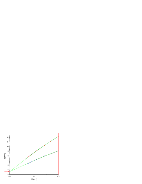
In favorable cases the ratio series $R(n+1)$ plotted as a function of $1/(n+1)$ can be extrapolated to infinite $n$ to estimate the critical temperature from the intercept, $1/w_{c}$, the critical exponent $\gamma$ from the initial slope $\partial R(n+1)/\partial(1/(n+1))=(\gamma-1)/w_{c}$, and the conformal correction exponent $\theta$ from the leading non-linear term. Unfortunately there can be parasitic oscillating terms in the ratios, arising from anti-ferromagnetic poles butera:02 , particularly in simple hypercubic lattices. It turns out that in the ISGs the parasitic terms in the susceptibility series become rather strong when the dimension drops. Explicit lists of terms for $\Gamma_{2}$ in dimension $d=4$ and below were tabulated in Ref. singh:86 .

For the simple hypercubic bimodal ISGs in general dimension Klein et al. klein:91 tabulated the terms to order 15 not only for the ISG susceptibility $\chi(w)$ series (called $\Gamma_{2}$ in their nomenclature) but also for the higher order susceptibilities $\Gamma_{3}$ and $\Gamma_{4}$ which they define. These susceptibilities have critical exponents $\gamma_{3}=(3\gamma+d\nu)/2$ and $\gamma_{4}=2\gamma+d\nu$ respectively klein:91 ; butera:02 . Unfortunately the parasitic terms are so strong in the $4$d $\Gamma_{2}$ susceptibility series that the ratios cannot be readily exploited so as to make accurate estimates of the critical parameters. This explains why the error bars quoted in Ref. daboul:04 for $\beta_{c}^{2}$ and $\gamma$ in $4$d are rather large. However, we have summed the tabulations of klein:91 for $\Gamma_{3}$ and $\Gamma_{4}$ to obtain the $a_{3}(n)$ and $a_{4}(n)$ for these series, and have found that for these higher order susceptibilities the ratios behave very regularly in dimension $4$ (and above), as can be seen in Fig. 8. Expression 21 can be applied to these ratios and reliable extrapolations can be made through which one can estimate $w_{c},\gamma(3),\gamma(4)$ and $\theta$. Optimal fits excluding the small $n$ values are

$$R(n+1)=4.60\left(1+\frac{5.3}{(n+1)}-\frac{4.0}{(n+1)^{2.35}}\right)$$ (22)

for $\Gamma_{3}$, and

$$R(n+1)=4.60\left(1+\frac{9.15}{(n+1)}-\frac{9.0}{(n+1)^{2.4}}\right)$$ (23)

for $\Gamma_{4}$. The joint intercept $1/w_{c}=1/\tanh^{2}(\beta_{c})=4.60(2)$ corresponds to $\beta_{c}=0.505(2)$, and the initial slopes correspond to $\gamma_{3}=(3\gamma+d\nu)/2=6.30(10)$ and $\gamma_{4}=2\gamma+d\nu=10.15(10)$. The leading correction terms have an exponent $\theta\approx 1.4$, and prefactors with negative sign. By inspection any hypothesis of another term (which would then be the true conformal correction to scaling) having a much lower exponent and with a prefactor of the opposite sign can once again be ruled out. There are no statistical errors as all points are exact; systematic errors arising from the extrapolation are small.

The exponents estimated above from the simulations and so quite independently from the HTSE data correspond to $\gamma_{3}=(3\gamma+4\nu)/2=6.3(1)$ and $\gamma_{4}=2\gamma+4\nu=9.92(15)$, and so are fully consistent with the HTSE values.

VII Gaussian interaction model

We will present equivalent data for the hypercubic ISG model with Gaussian interactions in dimension four. All the discussions above apply equally well to the Gaussian data. Corrections for the Gaussian model are in general much weaker than for the bimodal model. Unfortunately no HTSE higher order susceptibility data are available for the Gaussian model.

Figure 9: (Color online) The $4$d Gaussian ISG. FSS for the correlation length ratio $\xi(\beta,L)/L$ at fixed inverse temperatures $\beta=0.5625$, $0.5600$, $0.5575$, $0.5550$, $0.5525$, $0.5500$ from top to bottom, against $1/L^{1.3}$. Dashed line : critical behavior.

Figure 10: (Color online) The $4$d Gaussian ISG. FSS for the Binder cumulant $g(\beta,L)$ at fixed inverse temperatures $\beta=0.5625$, $0.5600$, $0.5575$, $0.5550$, $0.5525$, $0.5500$ from top to bottom, against $1/L^{1.3}$. Dashed line : critical behavior.

Figure 11: (Color online) The $4$d Gaussian ISG. Thermodynamic derivative peak $D_{\max}=[\partial U(\beta,L)/\partial\beta]_{\max}$ data for dimensionless observables $U=W_{q},h,g$ (black squares, blue circles, red triangles). The peak location $\beta_{\max}(L)$ against the inverse peak height $1/D_{\max}(L)$.

Figure 12: (Color online) The $4$d Gaussian ISG. The Binder cumulant derivative peak height maximum $[\partial g(\beta,L)/\partial\beta]_{\max}$ normalized by $L$, against $L$ (log-log scaling).

Figure 13: (Color online) The $4$d Gaussian ISG. The ratio $\chi(\beta,L)/(\xi(\beta,L)/\beta)^{2}$ as function of $\xi(\beta,L)/\beta$ (log-log scaling). Sizes $L=6,8,12$ from left to right.

Figure 14: (Color online) The $4$d Gaussian ISG. The effective exponent $\gamma(\tau)$ with $\beta_{c}=0.5555$. Sizes $L=12,10,9,8,7,6,5$ from left to right. The blue continuous curve is calculated from the tabulated HTSE terms in Ref. daboul:04 . The red arrow is the exact high temperature limit $\gamma(\tau=1)=2d\beta_{c}^{2}$.

Figure 15: (Color online) The $4$d Gaussian ISG. The effective exponent $\nu(\tau)$ with $\beta_{c}=0.5555$. Sizes $L=12,10,8,7,6,5,4$ from left to right. The red arrow is the exact Gaussian high temperature limit $\nu(\tau=1)=(d-1)\beta_{c}^{2}$.

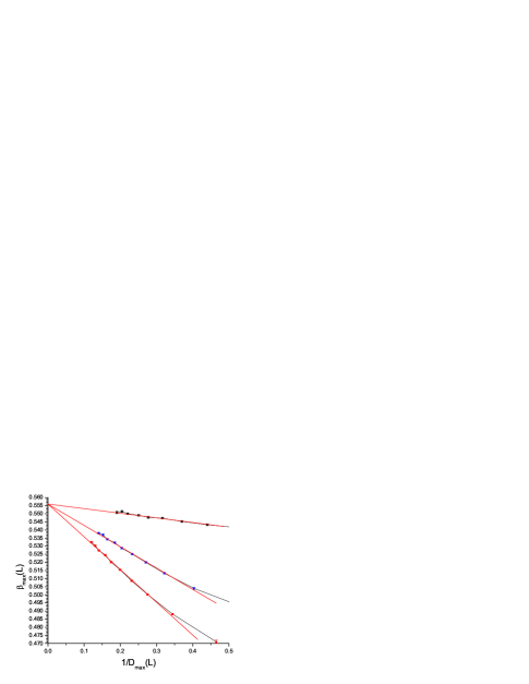
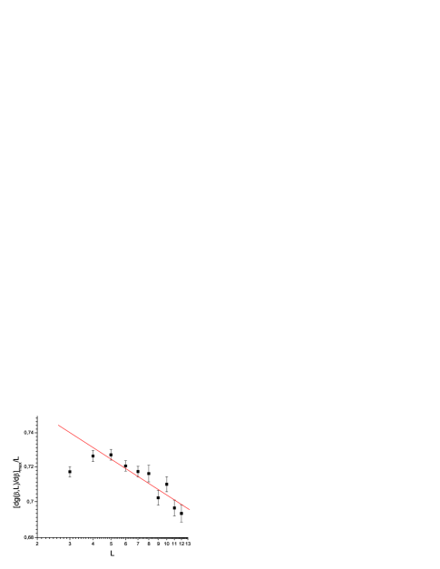
The $4$d Gaussian critical inverse temperature from both the FSS data, Figs. 9 and 10, and the thermodynamic derivative peak locations Fig. 11, is estimated to be $\beta_{c}=0.5555(10)$ or $T_{c}=1.800(3)$. This value is fully consistent with previous FSS estimates from Binder parameter and correlation length ratio measurements $0.555(3)$ parisi:96 ; ney:98 and 0.554(3)jorg:08 .

The Gaussian critical parameters for the normalised second moment correlation length $\xi(\beta,L)/L$ and the Binder cumulant $g(\beta,L)$ from Figs. 9 and 10 are $(\xi/L)_{c}=0.458(5)$ and $g_{c}=0.485(5)$ respectively. The value for the Binder cumulant is close to the estimate $g_{c}=0.470(5)$ given in Ref. jorg:08 .

The exponent $\nu$ estimated directly form the Binder cumulant thermodynamic derivative peak heights, Fig. 12, is $1.030(5)$. This value is fully consistent with the estimate $\nu=1.02(2)$ given in Ref. jorg:08 .

The plot of $\ln(y)$ against $\ln(x)$ with $y=\chi(\beta,L)/(\xi(\beta,L)/\beta)^{2}$ and $x=\xi(\beta,L)/\beta$, Fig. 13, is fitted with a single effective correction :

$$y(x)=1.2x^{0.305}\left(1-0.17x^{-1.4}\right)$$ (24)

corresponding to a critical exponent $\eta=-0.305(10)$. This value is again fully consistent with but more accurate than the estimate $\eta=-0.275(25)$ given by jorg:08 .

The fit to the ThL effective $\gamma(\tau)$ with a fixed $\beta_{c}=0.5555$, Fig. 14, corresponds to

$$\chi=1.01\tau^{-2.37}\left(1-0.010\tau^{10}\right)$$ (25)

so with a critical exponent $\gamma=2.37(2)$ and only a very weak high order correction term. The prefactor for the usual leading correction term appears to be accidentally very close to zero. A similar conclusion was reached from the FSS analysis of the $4$d Gaussian model in jorg:08 . The fit to the ThL effective $\nu(\tau)$ with fixed $\beta_{c}=0.5555$, Fig. 15, corresponds to

$$\xi(\beta)=0.934\tau^{-1.025}\beta\left(1+0.070\tau^{1.5}\right)$$ (26)

so a critical exponent $\nu=1.025(3)$ and a correction term with a similar exponent to the exponent of the bimodal model leading correction.

The critical constants and exponents for a $4$d diluted bimodal model Ref. jorg:08 were estimated to be $g(\beta_{c},\infty)=0.472(2)$, $(\xi/L)(\beta_{c},\infty)\approx 0.440$, $\gamma=2.33(6)$, and $\nu=1.025(15)$. Each of the diluted bimodal critical values is similar to that for the $4$d Gaussian model, but the diluted bimodal model and the standard bimodal model studied above have quite different critical properties.

VIII Conclusion

We compare in Table 1 the bimodal and Gaussian interaction distribution model estimates for each of the critical parameters and critical exponents studied above. For all the parameters and exponents the estimates for the two models are quite different, with in each case differences of the order of 10%.

Table 1: Values of the $4$d bimodal and Gaussian critical parameters and exponents.

Parameter	Bimodal	Gaussian
$\beta_{c}$	$0.505(1)$	$0.5555(10)$
$g(\beta_{c},\infty)$	$0.525(5)$	$0.485(5)$
$(\xi/L)(\beta_{c},\infty)$	$0.485(5)$	$0.458(5)$
$\gamma$	$2.70(3)$	$2.37(2)$
$\nu$	$1.113(1)$	$1.030(5)$
$\eta$	$0.42(2)$	$0.305(10)$

We conclude that in $4$d ISGs the critical exponents, like the values of the critical ordering parameters, depend on the form of the interaction distribution. ISGs in dimension four with different interaction distributions are clearly not in the same universality class.

IX Acknowledgements

The simulations were performed on resources provided by the Swedish National Infrastructure for Computing (SNIC) at High Performance Computing Center North (HPC2N) and at Chalmers Centre for Computational Science and Engineering (C3SE).

References

- (1) K.G. Wilson, Rev. Mod. Phys. 47, 773 (1975).
- (2) S. F. Edwards and P. W. Anderson, J. Phys. F: Met. Phys. 5, 965 (1975).
- (3) R. N. Bhatt and A. P. Young, Phys. Rev. B 37, 3707 (1988).
- (4) H. G. Katzgraber, M. Korner, and A. P. Young, Phys. Rev. B 73, 224432 (2006).
- (5) M. Hasenbusch, A. Pelissetto, and E. Vicari, Phys. Rev. B 78, 214205 (2008).
- (6) T. Jörg and H. G. Katzgraber, Phys. Rev. B 77, 214426 (2008).
- (7) H. G. Ballesteros, L. A. Fernández, V. Martín-Mayor, A. Muñoz Sudupe, G. Parisi, and J.J. Ruiz-Lorenzo, Phys. Rev. B 58, 2740 (1998).
- (8) P. Calabrese, V. Martín-Mayor, A. Pelissetto, and E. Vicari, Phys. Rev. E 68, 036136 (2003).
- (9) J. L. Cardy, J.Phys. A Math. Gen., 20, L891 (1987).
- (10) G. Parisi, R. Petronzio, and F. Rosati, Eur. Phys. J. B 21, 605 (2001).
- (11) M. Castellana, Eur. Phys. Lett. 95, 47014 (2011).
- (12) M. C. Angelini, G. Parisi, and F. Ricci-Tersenghi, Phys. Rev. B 87, 134201 (2013).
- (13) H. G. Ballesteros, L. A. Fernández, V. Martín-Mayor, A. Muñoz Sudupe, Phys. Letts. B 400, 346 (1997).
- (14) A. M. Ferrenberg and D. P. Landau, Phys. Rev. B 41, 5081 (1991).
- (15) R. A. Baños, L. A. Fernandez, V. Martin-Mayor, and A. P. Young, Phys. Rev. B 86, 134416 (2012).
- (16) P. H. Lundow and I. A. Campbell, arXiv:1402.1991.
- (17) C. de Dominicis, private communication (2004).
- (18) A. J. Bray, private communication (2004).
- (19) M. Baity-Jesi et al., Phys. Rev. B 88, 224416 (2013).
- (20) L. Klein, J. Adler, A. Aharony, A. B. Harris, Y. Meir, Phys. Rev. B 43, 11249 (1991).
- (21) D. Daboul, I. Chang and A. Aharony, Eur. Phys. J. B 41, 231 (2004).
- (22) P. H. Lundow and I. A. Campbell, unpublished.
- (23) M. Weigel and W. Janke, Phys. Rev. Lett. 102, 100601 (2009).
- (24) M. E. Fisher and R. J. Burford, Phys. Rev. 156,583 (1967).
- (25) F. Wegner, Phys. Rev. B 5, 4529 (1972).
- (26) S. Gartenhaus and W. S. McCullough, Phys. Rev. B 88, 11688 (1988).
- (27) P. Butera and M. Comi, Phys. Rev. B 65,144431 (2002).
- (28) R. Fisch and A. B. Harris, Phys. Rev. Lett. 38, 785 (1977).
- (29) R. R. P. Singh and S. Chakravarty, Phys. Rev. Lett. 57, 245 (1986).
- (30) I. A. Campbell, K. Hukushima, and H. Takayama, Phys. Rev. Lett. 97, 117202 (2006).
- (31) I. A. Campbell and P. Butera, Phys. Rev. B 78, 024435 (2008).
- (32) J. Kouvel and M. E. Fisher, Phys. Rev. A 136, 1626 (1964).
- (33) C. Domb and M. F. Sykes, Proc. Phys. Soc. A235, 247 (1956).
- (34) G. Parisi, F. Ricci-Tersenghi, and J. J. Ruiz-Lorenzo, J. Phys. A 29, 7943 (1996).
- (35) M. Ney-Nifle, Phys. Rev. B 57, 492 (1998).
- (36) H. G. Ballesteros, L. A. Fernández, V. Martín-Mayor, A. Muñoz Sudupe, G. Parisi, and J. J. Ruiz-Lorenzo, J. Phys. A 32, 1 (1999).
- (37) E. Gardner, J. Phys. 45, 1755 (1984).