3D Model Atmospheres for Extremely Low-Mass White Dwarfs
Abstract
We present an extended grid of mean three-dimensional (3D) spectra for low-mass, pure-hydrogen atmosphere DA white dwarfs (WDs). We use CO5BOLD radiation-hydrodynamics 3D simulations covering = 6000–11,500 K and = 5–6.5 ( in cm s-2) to derive analytical functions to convert spectroscopically determined 1D temperatures and surface gravities to 3D atmospheric parameters. Along with the previously published 3D models, the 1D to 3D corrections are now available for essentially all known convective DA WDs (i.e., = 5–9). For low-mass WDs, the correction in temperature is relatively small (a few per cent at the most), but the surface gravities measured from the 3D models are lower by as much as 0.35 dex. We revisit the spectroscopic analysis of the extremely low-mass (ELM) WDs, and demonstrate that the 3D models largely resolve the discrepancies seen in the radius and mass measurements for relatively cool ELM WDs in eclipsing double WD and WD + milli-second pulsar binary systems. We also use the 3D corrections to revise the boundaries of the ZZ Ceti instability strip, including the recently found ELM pulsators.
Subject headings:
convection – hydrodynamics – white dwarfs1. INTRODUCTION
Recent three dimensional (3D) radiation hydrodynamical simulations of the Sun and main-sequence stars have led to significant improvements in our knowledge of stellar atmospheres and spectroscopic abundance measurements (e.g. Asplund et al. 2009; Caffau et al. 2011; Scott et al. 2015a, b). The major differences between the 1D and 3D model atmospheres result from the insufficient description of convection by the mixing length theory (Böhm-Vitense 1958, MLT) that is used in the 1D models.
Convection becomes important in hydrogen-atmosphere (DA) white dwarfs (WDs) below about 15,000 K. Spectroscopic analyzes of large samples of WDs with 1D model atmospheres show the so-called “high problem” (Bergeron et al. 1990; Eisenstein et al. 2006; Kepler et al. 2007; Gianninas et al. 2011; Kleinman et al. 2013), where the spectroscopically determined masses of WDs cooler than 13,000 K are systematically higher than their hotter counterparts by as much as 20%. There is no known evolution effect or observational bias that should lead to such a change in mass for the cooler WDs, and a larger average mass is not observed for cool WDs with parallax measurements. In a series of papers, Tremblay et al. (2011, 2013a, 2013b, 2013c) presented the first 3D model atmosphere calculations for DA WDs using the CO5BOLD radiation-hydrodynamics code (Freytag et al. 2012). The predicted Balmer line profiles are significantly different in the 3D models, and the “high problem” essentially disappears in the spectroscopic analyzes based on the 3D models. The previously published model grid covers the effective temperature range of 6000-15,000 K and the surface gravity range of = 7–9. To study the effects of 3D models on the physical parameters of the extremely low-mass (ELM) WDs with , here we extend our 3D model atmosphere grid down to = 5.
ELM WDs are helium-core remnants and almost always found in short period binary systems. The ELM Survey (Brown et al. 2010; Kilic et al. 2010a; Gianninas et al. 2014a, and references therein) has discovered binaries with periods as short as 12–20 min (Brown et al. 2011; Kilic et al. 2014). Improving the constraints on the ELM WD physical parameters, including the spectroscopic mass and gravitational wave strain, is important for future gravitational wave missions in the milli-Hertz frequency range. In addition, all of the known eclipsing and/or tidally distorted double WD systems involve low-mass WDs. Studying the mass-radius relation for these systems, Gianninas et al. (2014a) and Kaplan et al. (2014) find that the 1D spectroscopic analysis underestimates the radius (or overestimates the surface gravity) for ELM WDs cooler than about 10,000 K. NLTT 11748 is an excellent example, where the eclipses constrain the radius and surface gravity to = 0.0423–0.0433 R☉ and = 6.32–6.38 (Kaplan et al. 2014), while the 1D spectroscopic analysis predicts = 6.83 (Gianninas et al. 2014a). Therefore, the “high problem” seems to impact all convective DA WDs, including ELM WDs.
We outline the details of our 3D model calculations in Section 2, and present the 1D to 3D atmospheric parameter correction functions for the extended range of in Section 3. We discuss the astrophysical implications, including the revised parameters for the ELM Survey sample, radius constraints from the eclipsing and tidally distorted systems as well as ELM WD + milli-second pulsar binaries, and the ZZ Ceti instability strip in Section 4. We conclude in Section 5.
2. 3D MODEL ATMOSPHERES
We have carried out 30 simulations of pure-hydrogen ELM WD atmospheres with CO5BOLD (Freytag et al. 2012). These 3D simulations in the range provide a direct extension to the grid presented in Tremblay et al. (2013c) for . The calculations also complement the CIFIST grid of CO5BOLD simulations for stars and giants (Ludwig et al. 2009b; Caffau et al. 2011) with . Figure 1 illustrates the new ELM WD 3D simulations in a HR-type diagram. Properties of the individual models, such as (derived from the temporally and spatially averaged emergent stellar flux), , box dimensions, and computation time, can be found in Table 1.

| (K) | (cm s-2) | (cm) | (cm) | (s) | (s) | |||
| 5977 | 5.00 | 7.56 | 8.38 | 6.58 | 2.96 | 4.00 | 1 | .17 |
| 6958 | 5.00 | 7.71 | 8.46 | 6.08 | 2.99 | 4.00 | 1 | .03 |
| 7513 | 5.00 | 7.62 | 8.33 | 5.64 | 2.99 | 4.00 | 0 | .92 |
| 8501 | 5.00 | 8.36 | 8.64 | 7.77 | 3.06 | 3.30 | 0 | .94 |
| 9001 | 5.00 | 8.38 | 8.64 | 5.46 | 3.00 | 3.30 | 1 | .19 |
| 9499 | 5.00 | 8.49 | 8.68 | 8.29 | 3.01 | 3.30 | 1 | .54 |
| 6044 | 5.50 | 7.04 | 7.66 | 6.98 | 2.97 | 3.50 | 0 | .75 |
| 6915 | 5.50 | 7.20 | 7.73 | 6.58 | 3.01 | 3.50 | 0 | .62 |
| 7967 | 5.50 | 7.37 | 7.98 | 6.57 | 3.02 | 3.50 | 0 | .47 |
| 8996 | 5.50 | 7.93 | 8.18 | 7.47 | 3.02 | 2.90 | 0 | .46 |
| 9499 | 5.50 | 7.93 | 8.18 | 6.12 | 3.00 | 2.90 | 0 | .67 |
| 9998 | 5.50 | 8.00 | 8.22 | 6.75 | 3.01 | 2.90 | 0 | .91 |
| 10500 | 5.50 | 8.06 | 8.29 | 7.23 | 3.01 | 2.90 | 1 | .40 |
| 5958 | 6.00 | 6.66 | 7.20 | 7.21 | 2.99 | 3.00 | 0 | .38 |
| 6971 | 6.00 | 6.78 | 7.28 | 6.99 | 3.02 | 3.00 | 0 | .21 |
| 7962 | 6.00 | 6.89 | 7.34 | 6.82 | 2.99 | 3.00 | 0 | .09 |
| 8963 | 6.00 | 7.00 | 7.42 | 5.76 | 2.96 | 3.00 | 0 | .08 |
| 9491 | 6.00 | 7.32 | 7.65 | 5.07 | 3.00 | 2.40 | 0 | .03 |
| 9999 | 6.00 | 7.46 | 7.71 | 7.34 | 3.00 | 2.40 | 0 | .21 |
| 10499 | 6.00 | 7.52 | 7.75 | 5.75 | 3.01 | 2.40 | 0 | .40 |
| 11001 | 6.00 | 7.49 | 7.75 | 5.00 | 2.96 | 2.40 | 0 | .77 |
| 5986 | 6.50 | 6.10 | 6.57 | 7.01 | 2.99 | 2.50 | 0 | .03 |
| 6922 | 6.50 | 6.20 | 6.65 | 7.48 | 3.00 | 2.50 | 0 | .19 |
| 7990 | 6.50 | 6.35 | 6.84 | 6.76 | 2.99 | 2.50 | 0 | .31 |
| 8907 | 6.50 | 6.51 | 7.03 | 6.66 | 3.00 | 2.50 | 0 | .42 |
| 9412 | 6.50 | 6.54 | 6.95 | 5.29 | 3.02 | 2.50 | 0 | .49 |
| 9989 | 6.50 | 6.95 | 7.24 | 6.75 | 3.02 | 2.50 | 0 | .49 |
| 10500 | 6.50 | 6.99 | 7.24 | 5.80 | 3.01 | 2.05 | 0 | .32 |
| 11000 | 6.50 | 7.05 | 7.28 | 5.77 | 3.01 | 2.05 | 0 | .13 |
| 11499 | 6.50 | 7.09 | 7.33 | 5.83 | 3.01 | 2.05 | 0 | .12 |
| 6011a | 5.00 | 8.04 | 8.08 | 7.93 | 8.38 | 5.00 | 1 | .08 |
|
aStellar simulation with = 8.51% and [M/H] = .
Notes. All quantities were averaged over 12 snapshots. is derived from the temporal and spatial average of the emergent flux, (same as ) and correspond to the geometrical dimensions of the box, and is the Rosseland optical depth averaged over constant geometrical depth. is the computation time in stellar time and is the advective or turnover timescale at the geometrical depth that corresponds to . |
||||||||
| Char. Size | Mach | |||||
| (K) | (cm s-2) | (cm) | (cm) | (s) | (%) | |
| 5977 | 5.00 | 7.50 | 6.70 | 1.53 | 16.91 | 0.42 |
| 6958 | 5.00 | 7.54 | 6.74 | 1.62 | 23.95 | 0.26 |
| 7513 | 5.00 | 7.57 | 6.77 | 1.65 | 23.17 | 0.12 |
| 8501 | 5.00 | 7.83 | 6.86 | 1.51 | 18.34 | 0.07 |
| 9001 | 5.00 | 7.69 | 6.92 | 1.45 | 11.17 | 0.26 |
| 9499 | 5.00 | 7.77 | 6.99 | 1.49 | 3.80 | 0.58 |
| 6044 | 5.50 | 6.78 | 6.21 | 1.12 | 13.00 | 0.50 |
| 6915 | 5.50 | 6.91 | 6.25 | 1.15 | 21.22 | 0.34 |
| 7967 | 5.50 | 7.08 | 6.31 | 1.17 | 23.14 | 0.14 |
| 8996 | 5.50 | 7.42 | 6.41 | 1.19 | 18.83 | 0.06 |
| 9499 | 5.50 | 7.27 | 6.47 | 0.98 | 13.01 | 0.22 |
| 9998 | 5.50 | 7.32 | 6.53 | 0.79 | 6.93 | 0.42 |
| 10500 | 5.50 | 7.46 | 6.62 | 0.80 | 1.84 | 0.86 |
| 5958 | 6.00 | 6.23 | 5.71 | 0.86 | 8.02 | 0.62 |
| 6971 | 6.00 | 6.40 | 5.77 | 0.80 | 17.55 | 0.43 |
| 7962 | 6.00 | 6.53 | 5.82 | 0.80 | 22.37 | 0.27 |
| 8963 | 6.00 | 6.63 | 5.88 | 0.80 | 21.21 | 0.04 |
| 9491 | 6.00 | 6.81 | 5.94 | 0.80 | 19.55 | 0.05 |
| 9999 | 6.00 | 6.82 | 6.01 | 0.58 | 13.76 | 0.24 |
| 10499 | 6.00 | 6.83 | 6.07 | 0.37 | 7.65 | 0.39 |
| 11001 | 6.00 | 6.81 | 6.15 | 0.64 | 2.13 | 0.73 |
| 5986 | 6.50 | 5.73 | 5.21 | 0.43 | 5.13 | 0.71 |
| 6922 | 6.50 | 5.89 | 5.28 | 0.37 | 12.49 | 0.52 |
| 7990 | 6.50 | 6.00 | 5.33 | 0.33 | 19.63 | 0.36 |
| 8907 | 6.50 | 6.13 | 5.38 | 0.37 | 21.18 | 0.21 |
| 9412 | 6.50 | 6.31 | 5.42 | 0.38 | 20.45 | 0.10 |
| 9989 | 6.50 | 6.47 | 5.48 | 0.30 | 19.67 | 0.06 |
| 10500 | 6.50 | 6.40 | 5.55 | 0.17 | 16.19 | 0.19 |
| 11000 | 6.50 | 6.35 | 5.60 | 0.00 | 9.80 | 0.35 |
| 11499 | 6.50 | 6.36 | 5.68 | 0.20 | 4.90 | 0.56 |
| 6011a | 5.00 | 7.34 | 6.60 | 1.76 | 17.79 | 0.38 |
|
aStellar simulation with = 8.51% and [M/H] = .
Notes. All quantities were averaged over 250 snapshots except (see Table 1). The characteristic horizontal size of the granulation, decay time, and relative intensity contrast () were computed from emergent intensity snapshots using the definitions given in Tremblay et al. (2013b). Both the pressure scale height () and the Mach number are computed at the geometrical depth that corresponds to . |
||||||
The numerical setup for the ELM WD simulations is the same as that described in Tremblay et al. (2013c) for a grid of points. The properties of the boundary conditions are reported in Freytag et al. (2012, see Sect. 3.2). The warmest simulations, represented by filled symbols in Figure 1, have a convective zone that is thinner than the vertical dimension of the atmosphere. In those cases, we use a bottom layer that is closed to convective flows with imposed zero vertical velocities. In cooler models, the convective flux is transported in and out of the domain through an open boundary. In all cases the lateral boundaries are periodic and the top boundary is open to material flows and radiation. We use the same equation-of-state (EOS) and opacity tables as those described in Tremblay et al. (2013c). In particular, we employ the Hummer & Mihalas (1988) EOS, the Stark broadening profiles of Tremblay & Bergeron (2009), and the quasi-molecular line opacity of Allard et al. (2004). The wavelength-dependent opacities are sorted in the 8 bin configuration discussed in Tremblay et al. (2013c).
2.1. Physical Properties
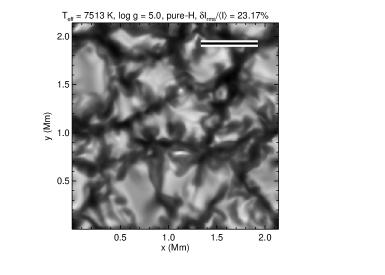
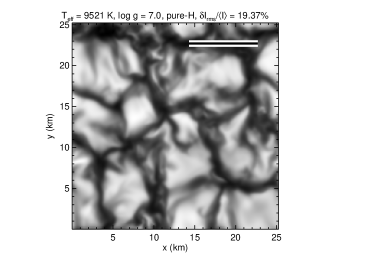
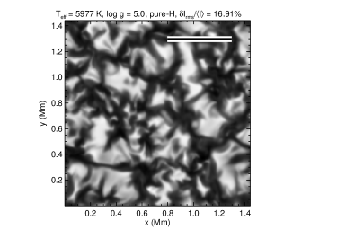
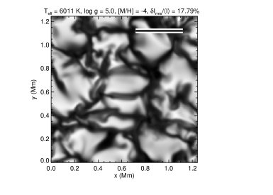
The ELM WD 3D simulations show physical properties that are very similar to those of the 3D models of higher mass WDs presented in earlier studies. Tremblay et al. (2013b) found that 3D effects on the thermal structure are well correlated with the density at Rosseland optical depth . Since the atmospheric density can be kept roughly constant by decreasing both and , the ELM simulations have properties similar to those of C/O-core WDs but with a shift towards smaller values.
Figure 2 compares our simulation at 7500 K and = 5.0 with the simulation at 9500 K and = 7.0 from Tremblay et al. (2013c). Both simulations have a similar relative intensity contrast and granulation is visually comparable. Table 2 demonstrates that ELM WDs have a slightly larger maximum relative intensity contrast compared to higher mass degenerates. ELM WDs are very similar to main-sequence simulations in that respect (see Figure 10 of Tremblay et al. 2013b). Furthermore, Table 2 describes the characteristic size of granulation and decay time. These quantities follow the same trends as those observed for higher mass WDs (Tremblay et al. 2013b), in particular the relation between the characteristic size of granulation to pressure scale height ratio and photospheric Mach number.
Our low gravity WD simulations reach photospheric plasma conditions and characteristic geometrical scales that are similar to main-sequence stars, although the radii are quite different. In order to better understand this link, we have computed a stellar model at 6000 K, , = 8.51%, and a metallicity of [M/H] = 4.0 based on solar elemental abundances from Grevesse & Sauval (1998) with updated CNO values (Asplund 2005). The model is an extension of the CIFIST grid for main-sequence stars where . The simulation is representative of the extremely metal-poor F-dwarfs with the currently highest derived surface gravities (Spite et al. 2012). The properties of the simulation are described in Tables 1 and 2, while Figure 3 shows the comparison with the pure-hydrogen ELM WD at 6000 K and = 5.0. The relative intensity contrast and size of the granules are similar, although the stellar atmosphere is denser by 58% at compared to the more opaque pure-hydrogen WD atmosphere. It implies that their properties are only expected to be qualitatively similar. Nevertheless, it demonstrates that ELM WDs will provide an important connection between WDs and main-sequence stars in future studies of the 3D effects on the determination of the atmospheric parameters from Balmer line profiles.
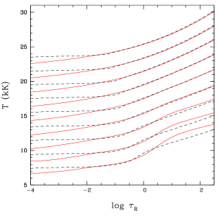
We have computed mean 3D structures, hereafter structures, which are spatial and temporal averages of and performed over surfaces of constant and for 12 random snapshots. We have employed those snapshots to define the values of our simulations (Table 1). In Figure 4, we compare the temperature structures of simulations and 1D models at 7000 K in the range . Convection is still fairly adiabatic in the photosphere for in this range, resulting in small differences between the and 1D cases except for the optically thin layers where 3D overshoot causes a significant dynamic cooling. Density decreases for lower surface gravities and convection becomes less efficient in the photosphere. Figure 4 demonstrates that differences between and 1D structures become larger for ELM WDs at 7000 K. The observed pattern is very similar to the one at constant and variable in Figure 7 of Tremblay et al. (2013a).
3. 3D ATMOSPHERIC PARAMETERS
3.1. Mean 3D Spectra
We have computed spectra from the 3D simulations in order to study the 3D effects on the determination of atmospheric parameters. First of all, we rely on mean spectra from structures, hereafter spectra. For WD simulations with , the normalized Balmer line profiles computed from structures are nearly identical to the results of a full 3D spectral synthesis (Tremblay et al. 2011, 2013c). However, we have found that the spectra approximation becomes questionable at lower gravities, in line with main-sequence simulations where 3D inhomogeneities have a significant direct impact on predicted Balmer line profiles (Ludwig et al. 2009a). We review first the differences between and 1D spectra and then consider the additional effects from 3D spectral synthesis in Sect. 3.2.
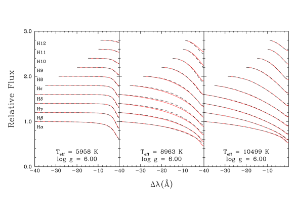
Figure 5 shows the comparison of predicted and 1D Balmer line profiles for three simulations at , which is an illustrative case for ELM WDs. The 1D spectra adopt the ML2/ = 0.8 parameterization of the MLT (Tremblay et al. 2010) and the same microphysics as the 3D calculations. The ELM results can be compared to the case at in Figure 16 of Tremblay et al. (2013a). One major difference is that up to ten Balmer lines are typically fitted simultaneously for ELM WDs, since the non-ideal effects and the sensitivity to surface gravity are shifted to higher Balmer lines (Gianninas et al. 2014a). For the simulation at K and in the middle panel of Figure 5, it is only for H10 and higher lines in the series that profiles become shallower than 1D profiles due to differences in the predicted non-ideal effects. The latter are very sensitive to the density stratification in the atmosphere (Tremblay et al. 2013c). The shape of the lower Balmer lines is also significantly different between and 1D spectra at intermediate , which is mostly responsible for shifts.
The and 1D Balmer lines become identical at high values (see the right panel of Figure 5). For ELM WDs, this transition appears at relatively low temperatures, and 3D effects are largely negligible on the thermal structures for K. Similarly to C/O-core WDs, convection becomes very inefficient in this regime and the thermal structure is essentially fixed by the radiation field, even though convective velocities are still large. For cool values, the left panel of Figure 5 suggests that 3D effects are small, but Section 3.2 demonstrates that the approximation is not always good in this regime.
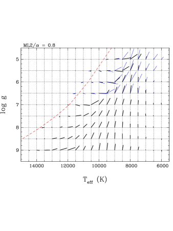
Figure 6 presents the atmospheric parameter corrections found by fitting the spectra with our standard grid of 1D spectra. The corrections were derived simultaneously for the nine Balmer lines from H to H12 in the same way we fit observations. The structures deviate significantly from their 1D counterparts in the upper layers () due to the cooling effect of convective overshoot. This results in deep cores for H and H, as observed in the middle panel of Figure 5. While we have no suggestion that the 3D simulations are inaccurate, there is no observational evidence for an adiabatic surface cooling in WDs and it appears premature to account for these effects. As a consequence, the line cores were partially removed from the fits, as well as the entire H line, as discussed in Sect. 3.1 of Tremblay et al. (2013c).
The atmospheric parameter corrections for ELM WDs in Figure 6 follow the trend observed for higher gravity objects, despite the fact that more lines are included in the fitting procedure in the former case. The corrections have a similar strength for ELM and C/O-core WDs, although they are restricted to a narrower range of at low surface gravity.
3.2. 3D Spectral Synthesis
We have employed the Linfor3D three-dimensional spectral synthesis code (Ludwig & Steffen 2008) to compute 3D H profiles for ELM white dwarfs. Unlike our previous experiments for , the 3D spectra and their counterparts from properly averaged structures differ by a few percent, with the largest effects at lower gravities. It is currently out of the scope of this work to proceed with the time-consuming computation of a full grid of 3D synthetic spectra. However, to further constrain the precision of the 3D corrections, we have recomputed our grid of ELM spectra with the so-called 1.5D approximation (Steffen et al. 1995). Under this formalism, we assume that the physical conditions do not vary in the horizontal direction for each point on the top of the computational box, i.e. each column is a plane-parallel atmosphere. The 1.5D spectrum is then the average over all columns, for which the emergent 1D spectra can be easily calculated from our regular spectral synthesis code. The full 3D spectral synthesis has the effect of coupling nearby grid points, hence it is expected to lie somewhere between the extreme cases of the 1.5D and approximations.
In Figure 6, we compare the 1.5D (blue) and (black) atmospheric parameter corrections. We notice that while the approximation is relatively good at , especially in terms of corrections, it becomes questionable at lower gravities. We remind the reader that the 1.5D approximation overestimates 3D effects, hence suggests an upper limit to the 3D corrections. Since both 1.5D and corrections have the same signs, we suggest that applying the corrections provides a minimum 3D effect and a reasonable estimate of the atmospheric parameters of ELM WDs.
The deficiency of the approximation for ELM WDs is likely explained by multiple factors. The temperature fluctuations are slightly larger at lower gravities although this could not alone explain the variations. On the other hand, we find that the line to continuum emergent intensity ratio has a significantly larger spatial variation for lower surface gravities. It implies that fluctuations are less likely to cancel in the 3D spectral synthesis. This could be related to the fact that broadening due to collisions with neutral atoms becomes increasingly important at the low values where strong 3D effects are observed in ELM WDs. Finally, we have verified that the approximation is not the cause for the slight residual bump in the 3D WD mass distribution at K (Tremblay et al. 2013c; Genest-Beaulieu & Bergeron 2014) or the presence of deep cores for the lower Balmer lines compared to 1D spectra. These features are also present when using 1.5D spectra.
3.3. 3D Correction Functions
| = 5.0 | = 5.5 | = 6.0 | = 6.5 | |
|---|---|---|---|---|
| (K) | (cm s-2) | (cm s-2) | (cm s-2) | (cm s-2) |
| 6000 | 6 | 12 | 13 | 24 |
| 6500 | 33 | 19 | 11 | 7 |
| 7000 | 64 | 6 | 5 | 21 |
| 7500 | 203 | 50 | 19 | 16 |
| 8000 | 460 | 202 | 105 | 66 |
| 8500 | 555 | 425 | 197 | 152 |
| 9000 | 288 | 564 | 338 | 154 |
| 9500 | 99 | 243 | 557 | 151 |
| 10000 | 0 | 155 | 237 | 466 |
| 10500 | 0 | 78 | 116 | 211 |
| 11000 | 0 | 0 | 136 | 13 |
| 11500 | 0 | 0 | 0 | 123 |
We have derived functions to convert 1D atmospheric parameters of ELM WDs ( 7.0) to their 3D counterparts. We have ensured that the transition is smooth at 7.0 with the functions already presented in Tremblay et al. (2013c), which are more precise in the range 7.0 9.0. Fortran 77 functions are available in the online Appendix A. One can also rely on the data from Tables 3 and 4 to derive alternative functions or request spectra to the authors. Our independent variables are defined as
| (1) |
| (2) |
and the fitting functions for the ML2/ = 0.8 parameterization of the MLT are given below with the numerical coefficients identified in Table 5.
| (3) |
| (4) |
| = 5.0 | = 5.5 | = 6.0 | = 6.5 | |
|---|---|---|---|---|
| (K) | (cm s-2) | (cm s-2) | (cm s-2) | (cm s-2) |
| 6000 | 0.010 | 0.019 | 0.017 | 0.018 |
| 6500 | 0.023 | 0.037 | 0.040 | 0.024 |
| 7000 | 0.128 | 0.117 | 0.122 | 0.134 |
| 7500 | 0.239 | 0.225 | 0.215 | 0.239 |
| 8000 | 0.218 | 0.316 | 0.315 | 0.350 |
| 8500 | 0.064 | 0.181 | 0.302 | 0.340 |
| 9000 | 0.035 | 0.054 | 0.199 | 0.283 |
| 9500 | 0.001 | 0.006 | 0.056 | 0.150 |
| 10000 | 0.000 | 0.044 | 0.021 | 0.004 |
| 10500 | 0.000 | 0.037 | 0.027 | 0.002 |
| 11000 | 0.000 | 0.000 | 0.034 | 0.007 |
| 11500 | 0.000 | 0.000 | 0.000 | 0.024 |
| Coefficient | Value | Coefficient | Value |
|---|---|---|---|
| () | () | ||
| a1 | 7.3801851E+00 | b1 | 5.1729169E02 |
| a2 | 6.0978389E01 | b2 | 2.8514123E+00 |
| a3 | 8.5916775E01 | b3 | 2.8616686E+00 |
| a4 | 7.2038240E+00 | b4 | 3.2487645E+00 |
| a5 | 1.1195542E01 | b5 | 7.3122419E02 |
| a6 | 8.2204863E03 | b6 | 3.5157643E02 |
| a7 | 1.0550418E01 | b7 | 2.0585494E+00 |
| a8 | 2.2982103E03 | b8 | 2.9195288E01 |
| a9 | 2.3313912E02 | b9 | 9.2196599E02 |
| a10 | 1.5513621E01 | b10 | 3.2042870E01 |
| a11 | 6.5429395E01 | b11 | 6.3154984E01 |
| a12 | 1.1711317E+00 | b12 | 8.3885527E01 |
| a13 | 2.8245633E03 | b13 | 1.0552187E04 |
4. ASTROPHYSICAL IMPLICATIONS
| Object | h | |||||||||||||||
| (K) | (cm s-2) | (M☉) | (pc) | (0.01R☉) | (Gyr) | (M☉) | (M☉) | (Gyr) | ||||||||
| J0112+1835 | 9740 | 140 | 5.77 | 0.05 | 0.160 | 662 | 98 | 8.63 | 1.07 | 1.8 | 0.62 | 0.03 | 0.85 | 0.04 | 2.68 | 22.40 |
| J0152+0749 | 10800 | 190 | 5.93 | 0.05 | 0.168 | 980 | 131 | 7.36 | 0.83 | 1.4 | 0.57 | 0.03 | 0.78 | 0.04 | … | 22.80 |
| J0345+1748 | 8560 | 120 | 6.51 | 0.04 | 0.181 | 175 | 34 | 3.91 | 0.41 | 3.9 | 0.76 | 0.03 | … | 7.18 | 22.16 | |
| J0745+1949 | 8230 | 130 | 5.91 | 0.07 | 0.156 | 300 | 56 | 7.28 | 1.07 | 3.6 | 0.10 | 0.01 | 0.12 | 0.02 | 5.80 | 22.65 |
| J0818+3536 | 10190 | 190 | 5.87 | 0.09 | 0.164 | 3388 | 640 | 7.76 | 1.26 | 1.7 | 0.25 | 0.04 | 0.33 | 0.06 | 9.30 | 23.47 |
| J0822+2753 | 8800 | 130 | 6.36 | 0.05 | 0.175 | 496 | 72 | 4.57 | 0.51 | 4.2 | 0.76 | 0.08 | 1.05 | 0.11 | 8.18 | 22.31 |
| J0849+0445 | 10020 | 150 | 6.27 | 0.06 | 0.176 | 1101 | 158 | 5.08 | 0.61 | 1.9 | 0.65 | 0.04 | 0.89 | 0.05 | 0.45 | 22.38 |
| J0900+0234 | 8330 | 130 | 5.96 | 0.07 | 0.155 | 618 | 113 | 6.83 | 0.99 | 3.8 | … | … | … | … | ||
| J1005+3550 | 9760 | 140 | 6.00 | 0.05 | 0.166 | 1231 | 392 | 6.72 | 0.79 | 2.1 | 0.19 | 0.02 | 0.24 | 0.02 | 10.63 | 23.12 |
| J1112+1117 | 9240 | 140 | 6.17 | 0.06 | 0.169 | 266 | 42 | 5.57 | 0.70 | 2.7 | 0.14 | 0.01 | 0.17 | 0.02 | 12.73 | 22.56 |
| J1443+1509 | 8970 | 130 | 6.44 | 0.06 | 0.181 | 557 | 85 | 4.24 | 0.51 | 3.5 | 0.84 | 0.12 | 1.17 | 0.17 | 3.82 | 22.25 |
| J1512+2615 | 11250 | 180 | 6.93 | 0.06 | 0.250 | 766 | 96 | 2.85 | 0.31 | 0.4 | 0.31 | 0.04 | 0.39 | 0.05 | … | 22.94 |
| J1518+0658 | 9650 | 140 | 6.68 | 0.05 | 0.197 | 309 | 41 | 3.38 | 0.35 | 0.9 | 0.58 | 0.03 | 0.78 | 0.04 | … | 22.42 |
| J1538+0252 | 10030 | 150 | 5.98 | 0.06 | 0.167 | 1154 | 180 | 6.90 | 0.92 | 1.9 | 0.76 | 0.06 | 1.06 | 0.09 | … | 22.86 |
| J1557+2823 | 12470 | 200 | 7.76 | 0.05 | 0.448 | 191 | 18 | 1.45 | 0.11 | 0.4 | 0.41 | 0.03 | 0.51 | 0.04 | … | 21.92 |
| J1614+1912 | 8700 | 170 | 6.32 | 0.13 | 0.172 | 207 | 54 | 4.73 | 1.00 | 4.1 | … | … | … | … | ||
| J1630+2712 | 10200 | 170 | 6.03 | 0.08 | 0.169 | 2161 | 374 | 6.56 | 0.99 | 1.8 | 0.52 | 0.04 | 0.70 | 0.06 | … | 23.13 |
| J1741+6526 | 10410 | 170 | 6.02 | 0.06 | 0.170 | 998 | 150 | 6.71 | 0.87 | 1.7 | 1.11 | 0.05 | 1.57 | 0.06 | 0.16 | 22.11 |
| J1840+6423 | 9120 | 140 | 6.34 | 0.05 | 0.177 | 740 | 109 | 4.70 | 0.54 | 3.3 | 0.65 | 0.03 | 0.88 | 0.04 | 4.78 | 22.47 |
| J21030027 | 9900 | 150 | 5.79 | 0.05 | 0.161 | 1253 | 177 | 8.47 | 1.01 | 1.8 | 0.71 | 0.04 | 0.98 | 0.05 | 5.73 | 22.72 |
| J21190018 | 9690 | 150 | 5.72 | 0.08 | 0.158 | 2835 | 507 | 9.09 | 1.38 | 1.7 | 0.74 | 0.04 | 1.03 | 0.05 | 0.58 | 22.82 |
| J2228+3623 | 7890 | 120 | 5.78 | 0.08 | 0.175 | 420 | 79 | 8.96 | 1.34 | 7.7 | … | … | … | … | ||
| J2236+2232 | 11310 | 170 | 6.54 | 0.04 | 0.182 | 355 | 43 | 3.81 | 0.40 | 1.1 | 0.39 | 0.03 | 0.51 | 0.04 | … | 22.79 |
| Notes. J0345+1748 is NLTT 11748 and J2236+2232 is LP 400-22. | ||||||||||||||||
4.1. The ELM WD Sample
Gianninas et al. (2014a) present a 1D spectroscopic analysis of 61 low-mass WDs identified in the ELM Survey. All but five of these objects are in confirmed binary systems with periods ranging from 12 min to about a day. The majority of these targets are warmer than 12,000 K, where the 3D corrections are negligible. However, there are 23 convective WDs that are in the right and range for 3D corrections to be significant. Table 6 presents the updated parameters for these 23 systems, including temperature, surface gravity, mass, radius, cooling age, merger time, and their gravitational wave strain. The corrections are largest at around 8000 K for low-mass WDs. Hence, the parameters for relatively cool objects like J0345+1748 (NLTT 11748) have changed significantly. Since the 3D corrections lower the estimated , they also imply lower masses and gravitational wave strains for these systems.
1D spectroscopic analysis of Gianninas et al. (2014a) find K and for NLTT 11748111The earlier analysis by Kilic et al. (2010b) found . However, this was based on older WD models without the improved Stark broadening profiles of Tremblay & Bergeron (2009).. The 1D to 3D corrections from our models revise these to K and , a change of 0.3 dex in surface gravity. Using the Althaus et al. (2013) evolutionary models, the revised mass, distance, and radius are , pc, and , respectively. Our distance estimate is in excellent agreement with the parallax measured at the USNO, mas. Kaplan et al. (2014) use high-quality photometry of NLTT 11748 to constrain the same parameters from the observed eclipses. Depending on the thickness of the surface hydrogen layer of the secondary (more massive) WD, they derive and . Our mass and radius measurements, including the 3D correction factors, are consistent with their results within the errors.
4.2. The Mass-Radius Relation
There are several tidally distorted and/or eclipsing ELM WD systems that provide model-independent constraints on the radii. NLTT 11748 is discussed above; it is an eclipsing system where the spectroscopically inferred radius from the 1D models were significantly smaller than the eclipse modelling suggested (Kaplan et al. 2014; Gianninas et al. 2014a). Studying the radius constraints on the ELM WD sample, Gianninas et al. (2014a) find that the agreement between the spectroscopically inferred radius and the model-independent values is quite good for K. However, there are four relatively cool objects, LP 400-22, NLTT 11748, J0745, and J0751, where the radius is underestimated or the mass/ is overestimated. Figure 7 shows the comparison of the updated radius measurements, including the 3D corrections, for the same 10 stars from Gianninas et al. (2014a). Table 7 provides the references for the different radius measurements. The agreement between the spectroscopic and photometric radii is now excellent over the temperature range 8,000–17,000 K. There are only two deviant points, LP 400-22 and J0745, and we refer the reader to Kilic et al. (2013) and Gianninas et al. (2014b), respectively, for further discussion of these objects. Ignoring LP 400-22 and J0745, the excellent agreement between the radius measurements from these two independent methods suggests that the 3D model correction factors presented in this paper have the right amplitude to account for the differences seen in the earlier analysis relying on 1D models. Finally, we note that this independent verification of 3D results is unique to ELM WDs and fairly different to the one presented in Tremblay et al. (2013c) for single C/O-core WDs with trigonometric parallax measurements.
| Object | Ref. | |||
| (K) | (0.01R☉) | (0.01R☉) | ||
| J00560611 | 12230 180 | 5.65 0.61 | 5.6 0.6 | 1 |
| J01061000 | 16970 260 | 6.42 0.68 | 6.3 0.8 | 1 |
| J01121835 | 9740 140 | 8.64 1.07 | 8.8 0.9 | 1 |
| J03451748 | 8560 120 | 3.91 0.41 | 4.23 0.10 | 2 |
| J06512844 | 16340 260 | 3.25 0.31 | 4.0 0.2 | 1 |
| J07451949 | 8320 130 | 7.28 1.07 | 17.6 | 3 |
| J07510141 | 15740 250 | 13.15 1.04 | 13.8 | 1 |
| J17416526 | 10410 170 | 6.71 0.87 | 7.6 0.6 | 1 |
| J21190018 | 9690 150 | 9.09 1.38 | 10.3 1.6 | 1 |
| J22362232 | 11310 170 | 3.81 0.40 | 9.9 | 4 |
|
References. (1) Hermes et al. (2014); (2) Kaplan et al. (2014); (3) this work; (4) Kilic et al. (2013). Spectroscopic parameters are taken from this work and Gianninas et al. (2014a).
Notes. See also Gianninas et al. (2014b) regarding the measurement uncertainties for J07451949. |
||||
4.3. ELM WDs with Milli-Second Pulsar Companions

There are several WD companions to milli-second pulsars with optical spectroscopy available in the literature. These WDs provide an independent method to estimate the mass of the neutron star through constraints on the mass of the WD and the semi-amplitude of the radial velocity variations. Hence, accurate mass (and ) measurements for the ELM WDs in these systems are crucial. Many of these WDs have temperatures in the range 8000-10,000 K, where 3D effects are significant.
PSR J0218+4232, J1012+5307, and J19093744 have companions with K and , based on 1D spectroscopic analyses (van Kerkwijk et al. 1996; Callanan et al. 1998; Bassa et al. 2003; Jacoby et al. 2005). The corrections in are on the order of 0.3 dex at these temperatures. For example, van Kerkwijk et al. (1996) derive K and for the ELM WD companion to PSR J1012+5307. Taking the 3D corrections into account brings down these values to K and . PSR 19115958A has a WD companion with K and (Bassa et al. 2006). The amplitude of the 3D corrections is lower at these temperatures, bringing down the temperature and surface gravity to 9780 K and , respectively.
PSR J1738+0333 is an excellent system where the mass, radius, and the surface gravity of the WD companion can be estimated from both optical spectroscopy/photometry and radio observations. Antoniadis et al. (2012) obtain K, , , and from optical spectroscopy. Interestingly, they also derive (from the orbital period decay rate of the binary, mass ratio, parallax, and photometry), (from the mass ratio and orbital decay rate of the binary), and (from photometry). The latter measurements are independent of the 1D spectroscopic analysis and imply a lower surface gravity and a larger radius for this ELM WD. These provide additional evidence for the “high problem” in 1D spectroscopic analysis of ELM WDs, though (admittedly) the errors in surface gravity and radius are relatively large. Based on the 3D corrections factors that we estimate, we revise the spectroscopic parameters of this companion to K and , which are consistent (within the errors) with estimated using the independent method. We note that this WD companion also happens to be a pulsating WD (Kilic et al. 2015).
4.4. The ZZ Ceti Instability Strip
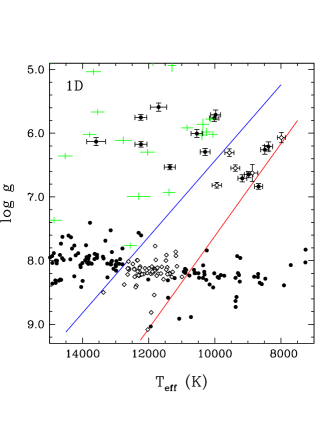
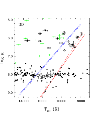
Figure 8 shows the instability strip for the pulsating DAV WDs based on 1D and 3D spectroscopic analyses. Here we only show the parameters for the DAVs derived from a uniform analysis by Gianninas et al. (2011, 2014a). We also show the five ELM pulsators currently known (excluding the companion to PSR J1738+0333 since the 1D model spectroscopic analysis of that star was not performed using the same models), and a large number of photometrically constant stars that help define the boundaries of the instability strip. The solid lines show the boundaries of the instability strip from Gianninas et al. (2014).
There is a clear trend of increasing with decreasing temperature in the 1D spectroscopic parameters of these stars. This trend disappears in the 3D version of the plot, where the 3D corrections lower the implied surface gravity. The blue edge of the instability strip is well defined in the 1D analysis. The 3D corrections move the stars systematically to slightly cooler temperatures and lower surface gravities. The dashed lines show the revised boundaries based on the 3D corrected parameters. For the blue edge, the boundary is simply shifted to the right by 100 K. The blue edge of the instability strip is still well defined for both normal mass and ELM WDs in the 3D analysis. For the red edge, as in the 1D case, we use GD 518 and SDSS J222859.93+362359.6 as the two anchor points at either extremity (the highest and lowest surface gravity) to define the 3D red edge, which now has a higher slope. The equations of the revised blue and red edges are defined by Equations 5 and 6, respectively. Given the small number of ELM pulsators currently known, it is too early to definitively constrain the red edge of the instability strip for those stars. The new ZZ Ceti instability strip from the 3D analysis does not reveal any new ELM pulsator candidates in the published list of ELM WDs, but the revised boundaries should be used in the future to look for new pulsating DA WDs.
| (5) |
| (6) |
5. CONCLUSIONS
We provide mean 3D model spectra for WDs with , extending the previously published 3D model grid to very low-mass WDs. Our 3D models now cover the entire temperature and surface gravity range for the observed population of convective DA WDs. We list 1D to 3D correction factors, which can be as large as 0.35 dex in surface gravity. These corrections largely resolve the discrepancies seen in the and radius estimates for relatively cool ELM WDs that are observed in double WD or WD + milli-second pulsar systems. We also update the boundaries of the ZZ Ceti instability strip for WDs, including the ELM pulsators as well as the normal () WDs.
References
- Allard et al. (2004) Allard, N. F., Kielkopf, J. F., & Loeillet, B. 2004, A&A, 424, 347
- Althaus et al. (2013) Althaus, L. G., Miller Bertolami, M. M., & Córsico, A. H. 2013, A&A, 557, AA19
- Antoniadis et al. (2012) Antoniadis, J., van Kerkwijk, M. H., Koester, D., et al. 2012, MNRAS, 423, 3316
- Asplund (2005) Asplund, M. 2005, ARA&A, 43, 481
- Asplund et al. (2009) Asplund, M., Grevesse, N., Sauval, A. J., & Scott, P. 2009, ARA&A, 47, 481
- Bassa et al. (2003) Bassa, C. G., van Kerkwijk, M. H., & Kulkarni, S. R. 2003, A&A, 403, 1067
- Bassa et al. (2006) Bassa, C. G., van Kerkwijk, M. H., Koester, D., & Verbunt, F. 2006, A&A, 456, 295
- Bergeron et al. (1990) Bergeron, P., Wesemael, F., Fontaine, G., & Liebert, J. 1990, ApJ, 351, L21
- Böhm-Vitense (1958) Böhm-Vitense, E. 1958, ZAp, 46, 108
- Brown et al. (2010) Brown, W. R., Kilic, M., Allende Prieto, C., & Kenyon, S. J. 2010, ApJ, 723, 1072
- Brown et al. (2011) Brown, W. R., Kilic, M., Hermes, J. J., et al. 2011, ApJ, 737, LL23
- Caffau et al. (2011) Caffau, E., Ludwig, H.-G., Steffen, M., Freytag, B., & Bonifacio, P. 2011, Sol. Phys., 268, 255
- Callanan et al. (1998) Callanan, P. J., Garnavich, P. M., & Koester, D. 1998, MNRAS, 298, 207
- Eisenstein et al. (2006) Eisenstein, D. J., Liebert, J., Harris, H. C., et al. 2006, ApJS, 167, 40
- Freytag et al. (2012) Freytag, B., Steffen, M., Ludwig, H.-G., et al. 2012, Journal of Computation al Physics, 231, 919
- Genest-Beaulieu & Bergeron (2014) Genest-Beaulieu, C., & Bergeron, P. 2014, ApJ, 796, 128
- Gianninas et al. (2011) Gianninas, A., Bergeron, P., & Ruiz, M. T. 2011, ApJ, 743, 138
- Gianninas et al. (2014a) Gianninas, A., Dufour, P., Kilic, M., et al. 2014a, ApJ, 794, 35
- Gianninas et al. (2014b) Gianninas, A., Hermes, J. J., Brown, W. R., et al. 2014b, ApJ, 781, 104
- Grevesse & Sauval (1998) Grevesse, N., & Sauval, A. J. 1998, Space Sci. Rev., 85, 161
- Hermes et al. (2013) Hermes, J. J., Montgomery, M. H., Winget, D. E., et al. 2013, ApJ, 765, 102
- Hermes et al. (2014) Hermes, J. J., Brown, W. R., Kilic, M., et al. 2014, ApJ, 792, 39
- Hummer & Mihalas (1988) Hummer, D. G., & Mihalas, D. 1988, ApJ, 331, 794
- Jacoby et al. (2005) Jacoby, B. A., Hotan, A., Bailes, M., Ord, S., & Kulkarni, S. R. 2005, ApJ, 629, L113
- Kaplan et al. (2014) Kaplan, D. L., Marsh, T. R., Walker, A. N., et al. 2014, ApJ, 780, 167
- Kepler et al. (2007) Kepler, S. O., Kleinman, S. J., Nitta, A., et al. 2007, MNRAS, 375, 1315
- Kilic et al. (2010a) Kilic, M., Brown, W. R., Allende Prieto, C., Kenyon, S. J., & Panei, J. A. 2010a, ApJ, 716, 122
- Kilic et al. (2010b) Kilic, M., Allende Prieto, C., Brown, W. R., et al. 2010b, ApJ, 721, L158
- Kilic et al. (2013) Kilic, M., Gianninas, A., Brown, W. R., et al. 2013, MNRAS, 434, 3582
- Kilic et al. (2014) Kilic, M., Brown, W. R., Gianninas, A., et al. 2014, MNRAS, 444, L1
- Kilic et al. (2015) Kilic, M., Hermes, J. J., Gianninas, A., & Brown, W. R. 2015, MNRAS, 446, L26
- Kleinman et al. (2013) Kleinman, S. J., Kepler, S. O., Koester, D., et al. 2013, ApJS, 204, 5
- Ludwig & Steffen (2008) Ludwig, H.-G., & Steffen, M. 2008, in Precision Spectroscopy in Astrophysics, ed. N.C. Santos, L. Pasquini, A.C.M. Correia, & M. Romanielleo (Berlin: Springer), 133
- Ludwig et al. (2009a) Ludwig, H.-G., Behara, N. T., Steffen, M., & Bonifacio, P. 2009a, A&A, 502, L1
- Ludwig et al. (2009b) Ludwig, H.-G., Caffau, E., Steffen, M., et al. 2009b, Mem. Soc. Astron. Italiana, 80, 711
- Scott et al. (2015a) Scott, P., Grevesse, N., Asplund, M., et al. 2015a, A&A, 573, A25
- Scott et al. (2015b) Scott, P., Asplund, M., Grevesse, N., Bergemann, M., & Sauval, A. J. 2015b, A&A, 573, A26
- Spite et al. (2012) Spite, M., Andrievsky, S. M., Spite, F., et al. 2012, A&A, 541, A143
- Steffen et al. (1995) Steffen, M., Ludwig, H.-G. & Freytag, B. 1995, A&A, 300, 473
- Tremblay & Bergeron (2009) Tremblay, P.-E., & Bergeron, P. 2009, ApJ, 696, 1755
- Tremblay et al. (2010) Tremblay, P.-E., Bergeron, P., Kalirai, J. S. & Gianninas, A. 2010, ApJ, 712, 1345
- Tremblay et al. (2011) Tremblay, P.-E., Ludwig, H.-G., Steffen, M., Bergeron, P., & Freytag, B. 2011, A&A, 531, L19
- Tremblay et al. (2013a) Tremblay, P.-E., Ludwig, H.-G., Steffen, M., & Freytag, B. 2013a, A&A, 552, A13
- Tremblay et al. (2013b) Tremblay, P.-E., Ludwig, H.-G., Freytag, B., Steffen, M., & Caffau, E. 2013b, A&A, 557, A7
- Tremblay et al. (2013c) Tremblay, P.-E., Ludwig, H.-G., Steffen, M., & Freytag, B. 2013c, A&A, 559, A104
- van Kerkwijk et al. (1996) van Kerkwijk, M. H., Bergeron, P., & Kulkarni, S. R. 1996, ApJ, 467, L89