Testing a Solar Coronal Magnetic Field Extrapolation Code with the Titov–Démoulin Magnetic Flux Rope Model

Abstract

In the solar corona, magnetic flux rope is believed to be a fundamental structure accounts for magnetic free energy storage and solar eruptions. Up to the present, the extrapolation of magnetic field from boundary data is the primary way to obtain fully three-dimensional magnetic information of the corona. As a result, the ability of reliable recovering coronal magnetic flux rope is important for coronal field extrapolation. In this paper, our coronal field extrapolation code (CESE–MHD–NLFFF, Jiang & Feng 2012) is examined with an analytical magnetic flux rope model proposed by Titov & Démoulin (1999), which consists of a bipolar magnetic configuration holding an semi-circular line-tied flux rope in force-free equilibrium. By using only the vector field in the bottom boundary as input, we test our code with the model in a representative range of parameter space and find that the model field is reconstructed with high accuracy. Especially, the magnetic topological interfaces formed between the flux rope and the surrounding arcade, i.e., the “hyperbolic flux tube” and “bald patch separatrix surface”, are also reliably reproduced. By this test, we demonstrate that our CESE–MHD–NLFFF code can be applied to recovering magnetic flux rope in the solar corona as long as the vector magnetogram satisfies the force-free constraints.

1 Introduction

The magnetic field plays a fundamental role in all physical processes in the Sun’s corona, such as the formation of coronal loops and prominences (or filaments), the production of solar flares, filament eruptions, and coronal mass ejections, as well as the determination of the structure of solar wind (Solanki et al. 2006). However, it is very difficult to make a direct measurement of the coronal magnetic field. Works that have been done to measure the coronal fields using the radio and infrared wave bands (e.g., Gary & Hurford 1994; Lin et al. 2004) can only give fragmentary and occasional data. Up to the present, the routine measurement of the Sun’s magnetic field that we can rely on is restricted to the solar surface, i.e., the photosphere. This is extremely unfortunate since the role of the magnetic field playing in the corona is much more important than that in the photosphere. As a result, our knowledge of the three-dimensional (3D) coronal magnetic field is largely based on extrapolations from photospheric magnetograms using some kind of reasonable physical models. In the low corona where the plasma $\beta$ (the ratio of gas pressure to magnetic pressure) is rather small $(\sim 0.01)$, the magnetic field can be well assumed as free of Lorentz force in the case of quasi-static state (i.e., ${\mathbf{J}}\times{\mathbf{B}}={\mathbf{0}}$ where ${\mathbf{J}}=\nabla\times\mathbf{B}$ is the current and ${\mathbf{B}}$ is the magnetic field). Thus the force-free field model is usually adopted in coronal field extrapolations.

Owing to the difficulty of direct solving the force-free equation $(\nabla\times\mathbf{B})\times{\mathbf{B}}={\mathbf{0}}$ which is intrinsically nonlinear, a variety of numerical codes have been proposed for nonlinear force-free field (NLFFF) extrapolations (e.g., see review papers by Schrijver et al. (2006), Metcalf et al. (2008), Wiegelmann (2008)). For faster convergence and better accuracy over the available codes, the authors have developed a new extrapolation code called CESE–MHD–NLFFF (Jiang et al. 2011; Jiang & Feng 2012), which is based on magnetohydrodynamics (MHD) relaxation method and an advanced numerical scheme, the spacetime conservation-element/solution-element (CESE) method. We have also critically examined our code with several NLFFF benchmark models and compared the results with previous joint studies by Schrijver et al. (2006) and Metcalf et al. (2008), which demonstrates its performance. The code has also been extended to application in spherical geometry and seamless full-sphere extrapolation for the global corona (Jiang et al. 2012b).

Coronal magnetic flux rope (MFR) is of great interest in the study of solar eruptive activities like filament eruption and CMEs. It is believed to be a good candidate for the critical pre-eruptive structures of storing magnetic free energy and helicity and holding cold dense filament material against gravity, while its instabilities can account for triggering and driving of eruptions. Observationally, a sequence of evidences such as the coronal sigmoid (Rust & Kumar 1996; Canfield et al. 1999), coronal hot channels (Zhang et al. 2012; Cheng et al. 2013), and coronal cavities (Gibson et al. 2006; Régnier et al. 2011) all suggested the existence of pre-eruptive MFR. Theoretically, MFR is an essential building block of many flare and CME models (e.g., Forbes & Isenberg 1991; Chen & Shibata 2000; Wu et al. 2000; Török & Kliem 2005; Kliem & Török 2006). In the coronal field extrapolations, it has been reported frequently that MFRs consistent with observations are reconstructed from relevant photospheric magnetograms (e.g., Canou & Amari 2010; Cheng et al. 2010; Guo et al. 2010; Jing et al. 2010; Guo et al. 2013; Jiang et al. 2014, 2014). Although many NLFFF codes has been demonstrated with the ability of extrapolating MFR, the reliability is still not fully approved. Thus, in the paper, we examine the reliability of our CESE–MHD–NLFFF code for extrapolating coronal MFR using an analytic force-free model proposed by Titov & Démoulin (1999, hereafter TD model). The remainder of the paper is organized as follows. Section 2 describes briefly the CESE–MHD–NLFFF code. The TD model is described in Section 3. Extrapolated result are shown in Section 4 and our conclusions are summarized in Section 5.

2 The CESE–MHD–NLFFF Code

In using the MHD relaxation approach for achieving a NLFFF, one usually starts from a potential field model matching the vertical component of the magnetogram, then replaces the transverse fields on bottom boundary with those from vector magnetogram (which is obviously inconsistent with the potential value, thus drives the system to evolve dynamically), and finally lets the MHD system to seek a new equilibrium in which all the other forces are negligible if compared with the Lorentz force. Consequently the Lorentz force must be nearly self-balancing and the final field can be regarded as the target solution of magnetic force-freeness. In our CESE–MHD–NLFFF code, we solve a simplified zero-$\beta$ MHD model with a fictitious frictional force, which is used to assure that a final equilibrium can be reached in a smooth way (Roumeliotis 1996; Valori et al. 2007). The specific equation is written in the following form with magnetic splitting

$$\frac{\partial\rho\mathbf{v}}{\partial t}=(\nabla\times\mathbf{B}_{1})\times\mathbf{B}-(\nabla\cdot\mathbf{B}_{1}){\mathbf{B}}-\nu\rho\mathbf{v},$$

$$\frac{\partial\mathbf{B_{1}}}{\partial t}=\nabla\times(\mathbf{v}\times\mathbf{B})+\nabla(\mu\nabla\cdot\mathbf{B}_{1})-\mathbf{v}\nabla\cdot\mathbf{B}_{1},$$

$$\rho=|{\mathbf{B}}|^{2},\ \ \mathbf{B}=\mathbf{B}_{0}+\mathbf{B}_{1}$$ (1)

where the total magnetic field ${\mathbf{B}}$ is split into ${\mathbf{B}}_{0}$, a potential field matching the normal component of the magnetogram, and ${\mathbf{B}}_{1}$, the deviation between ${\mathbf{B}}$ and ${\mathbf{B}}_{0}$. The last two terms in the induction equation are used to suppress the numerical errors of magnetic divergence (i.e., numerically induced magnetic monopole). $\nu$ is the frictional coefficient and $\mu$ is the diffusive speed of the numerical magnetic monopole. The value of them are given by $\nu=1/(5\Delta t)$ and $\mu=0.4(\Delta x)^{2}/\Delta t$ in the code, respectively, where $\Delta t$ is the time step and $\Delta x$ is the grid size. More details and the advantages of using above equations can be found in (Jiang & Feng 2012; Jiang et al. 2012b).

As the above equation system is just a simplified subset of the full MHD system, any available MHD code can be used to solve it. By taking into account the computational efficiency and accuracy, we prefer to utilize modern codes for MHD. However, most of the modern MHD codes are based on theory of characteristic decomposition of a hyperbolic system, and they are not suitable for Equation 2, because it is not a hyperbolic system. We thus select the CESE–MHD scheme (Jiang et al. 2010), which is free of characteristic decomposition and is very suitable for Equation 2. Furthermore, the CESE–MHD code has been successfully applied in solving many relevant problems in solar physics, e.g., the dynamic evolution of AR using data-driven MHD model (Jiang et al. 2012a), the global corona structure (Feng et al. 2012) and the interplanetary solar wind modeling (Feng et al. 2012; Yang et al. 2012).

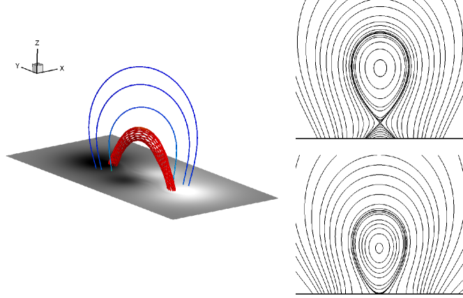
Figure 1: Left: basic magnetic configuration of TD model, the flux rope is shown with the red lines, the overlying near-potential arcades with blue lines, and the grey image shows the normal magnetogram on the bottom. Right: central vertical cross section of TD models with HFT (top, the 2D field lines form a X-point up in the corona) and with BP (bottom, the 2D field lines form a tangency point with the photosphere), illustrating two different stages of an emerging flux rope, fully emerged and partial emerged, respectively.

3 The TD Flux Rope Model

The TD flux rope model has gained considerable interest because of its relevance to the structures of solar active regions and eruptive magnetic field, which is demonstrated by many investigations (Roussev et al. 2003; Török et al. 2004; Török & Kliem 2005; Schrijver et al. 2008; McKenzie & Canfield 2008; Titov et al. 2014). Basically, the TD model is constructed to simulate an bipolar active region containing a half-buried, toroidal current-carrying flux rope balanced (or confined) by the overlying arched near-potential field (as shown in Figure 1). Excessive twist of the flux rope can trigger its kink instability (Török & Kliem 2005), and a too fast decaying of the overlying field with height can trigger the torus instability of the system (Kliem & Török 2006). With the change of its parameters, the model can also be used to illustrate different stages of an twisted sub-photospheric flux tube emerging bodily into the corona (see Figure 7 of Gibson et al. 2006). As shown in Figure 1, two different configurations, the one with a bald patch separatrix surface (BPSS), and the one without BPSS but with a hyperbolic flux tube (HFT), show the stages of partial and full emergence of flux rope, respectively. The reader is referred to (Titov & Démoulin 1999; Titov et al. 2014; Valori et al. 2010) for detailed description of the model and its parameter settings.

By only using the magnetic field on the model’s bottom boundary to reconstruct the flux rope, the TD model represents a far more difficult challenge of extrapolation than those simple sheared field models (e.g., the force-free field model by Low & Lou 1990). As examined by Wiegelmann et al. (2006) and Valori et al. (2010), this model requires a topological change from the initial potential field to obtain the flux-rope configuration. Valori et al. (2010) has extensively tested their extrapolation code using the TD model with a series of parameter sets, which includes four sets of stable model. They are, respectively, a Low-HFT case, a High-HFT case, a No-HFT case and a BP case. An HFT is present in the first two cases, one with the HFT very close to the photosphere (Low-HFT) and the other with the HFT reaching significantly into the volume (High HFT). The No-HFT case has no HFT present above the photosphere, hence, its magnetic topology is much simpler than the first two cases. These three configurations have no bald patch at the photosphere because the toroidal field component is relatively strong. For the BP case, the flux rope has a left-handed average twist of about $2\pi$, which is close to the twist of the first three equilibria, but a BPSS is introduced in the resulting field by enlarging the minor radius of the torus. Here we use exactly the same reference data from Valori et al. (2010)’s paper with the same grid resolution $\Delta=0.06$ and extrapolation box of interest, $[-3.03,3.03]\times[-4.95,4.95]\times[-0.06,4.44]$, while our actual computational volume is several times larger than the extrapolation volume of interest to minimize the numerical boundary effects.

Because the analytical TD solutions are approximately force-free, Valori et al. (2010) relaxed them to numerical equilibria using the MHD code of Török & Kliem (2003), which results in only little change to the geometry shape of the flux rope but improves the force-freeness for the models. Even though, we should point out that these reference models are still not perfect force-free solutions for the following reasons. Firstly, the data contains strong numerical oscillation, for example, see Figure 2. Although not obvious in tracing the field lines which are integral result of the field data, the oscillation is obvious when make numerical difference on the data. This oscillation is resulted from the MHD relaxation of the analytic TD model by the Török & Kliem (2003)’s code. Secondly, the bottom magnetograms (i.e., the vector field on the bottom boundary of model data) contains force that cannot be ignored. To assess the force-free quality of the magnetograms, we calculated the same metrics $\epsilon_{\rm flux}$, $\epsilon_{\rm force}$ and $\epsilon_{\rm torque}$ as in (Wiegelmann & Neukirch 2006; Jiang & Feng 2013), which measure flux, force, and torque imbalance of the magnetogram. As can be seen, the force-freeness is fulfilled well by the first three cases, but not that well for the BP case (note that both parameters $\epsilon_{\rm force}$ and $\epsilon_{\rm torque}$ is above 0.01), which can cause non-negligible inconsistence in the NLFFF extrapolation. For these reasons, a perfect extrapolation does not necessarily mean to reproduce a magnetic field matching perfectly the reference model.

Table 1: Quality of the magnetograms: normalized flux $\epsilon_{\rm flux}$, force $\epsilon_{\rm force}$, and torque $\epsilon_{\rm torque}$ imbalance as defined in (Wiegelmann & Neukirch 2006).

Case	$\epsilon_{\rm flux}$	$\epsilon_{\rm force}$	$\epsilon_{\rm torque}$
High_HFT	1.30E-08	3.45E-03	5.48E-03
Low_HFT	-3.63E-08	5.88E-03	8.88E-03
No_HFT	5.83E-09	7.29E-03	1.09E-02
BP	2.08E-08	1.46E-02	2.09E-02

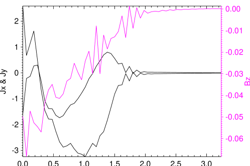
Figure 2: Numerical oscillation of the reference data of the TD model: $J_{x},J_{y}$ and $B_{z}$ along the vertical grid line of $x=-0.03,y=-0.03$ in the High_HFT case.

4 Results

Same as Valori et al. (2010), the extrapolation results are analyzed within a central region of the extrapolation box by discarding 20 grid layers of its top and lateral boundaries. The metrics for accessing the extrapolation quality are defined as Jiang & Feng (2013). Similarly, we measure the degree of force-freeness by the current-weighted (and current-square-weighted) average sine-angle between magnetic field and current,

$${\rm CWsin}\equiv\frac{\int_{V}{J}\sigma dV}{\int_{V}{J}dV};\ \ {\rm C^{2}Wsin}\equiv\frac{\int_{V}J^{2}\sigma dV}{\int_{V}J^{2}dV},\ \ \sigma=\frac{|{{\mathbf{J}}}\times{{\mathbf{B}}}|}{{J}{B}}.$$ (2)

The solenoidal property is quantified by

$$\langle|f_{i}|\rangle=\frac{1}{V}\int_{V}\frac{\nabla\cdot\mathbf{B}}{6B/\Delta x}dV.$$ (3)

The mean relative error between the extrapolated field ${\mathbf{B}}$ and the original reference field ${\mathbf{B}}_{\rm ref}$,

$$E_{\rm M}=\frac{1}{V}\int_{V}\frac{|{\mathbf{B}}^{\rm ref}-{\mathbf{B}}|}{|{\mathbf{B}}^{\rm ref}|}.$$ (4)

In order to reliably compare the reference and the extrapolated fields and their qualities of force-freeness, we use a fourth-order difference of ${\mathbf{B}}$ to calculate the current ${\mathbf{J}}$ and $\nabla\cdot\mathbf{B}$. Besides, to judge the magnetic topology, we compute the relative errors of the apex heights of the flux rope axis (FRA) and the HFT (if present) between the extrapolated and reference fields. Since the flux rope writhes only slightly out of the plane ${x=0}$ in the models considered in this paper, both of the apex heights can be approximately as the inversion points of $B_{x}(0,0,z)$, which is a good approximation of the poloidal component of the field at the line-symmetric $z$ axis. Finally we compute the relative errors of the magnetic energy ($E_{\rm mag}$) between the extrapolated and reference fields.

The results are given in Table 2. Regarding the metrics of force-freeness and divergence-freeness, the extrapolation code achieves solutions slightly even better than the reference models for the first three cases. Since both the models (i.e., the reference model and the extrapolation) are produced by numerical codes, it is suggested that our code performs better in relaxing the magnetic field to a force-free and divergence-free solution. For the first three cases, the mean relative errors $E_{\rm m}$ are only several percents, demonstrating that the reference models are reproduced with very high accuracy. The topology parameters, e.g., apex of FRA and HFT are very close to those of the reference model, except for the HFT apex of the low HFT case with a relative error of fifteen percent. This is because in the low HFT case the HFT is rather low with only about one grid point from the bottom, thus the size of the grid is not sufficiently small to resolve the HFT. The force-freeness for the BP case is not as good as the first three cases, and consequently the topology of the extrapolated field also deviates considerably from the reference model. This is as expected because we have shown that the magnetogram of the BP case is most inconsistent with the force-free constraints (Table 1). For all the cases, the energy content is well recovered with relative errors below several percents.

Table 2: Results for the metrics of extrapolations

Figure of merit	High_HFT	Low_HFT	No_HFT	BP
CWsin $\times 10^{2}$	2.07/2.59	2.04/2.34	2.25/1.94	5.41/0.81
C2Wsin $\times 10^{2}$	1.04/1.24	0.82/1.08	0.77/0.91	2.50/0.41
$<|f_{i}|>\times 10^{5}$	4.06/6.52	3.28/6.45	3.52/5.74	12.7/7.57
$E_{\rm M}$	0.020	0.015	0.016	0.116
HFT apex	5.18%	15.5%	…	…
FRA apex	5.03%	1.38%	0.05%	22.1%
$E_{\rm mag}$	0.75%	0.98%	1.1%	2.1%

0.86For the first three metrics, results of the reference models are also given following those of the extrapolations.

For a visual inspection of the magnetic configuration, we show selected field lines of two cases, the High_HFT and No_HFT, in Figures 3 and 4, respectively. The field lines for all models are traced from the same set of points in the central cross section of the volume. The field lines include the flux rope axis, four field lines closely around the rope axis, one low-lying below the flux rope and two highly overlying the flux rope. The field lines are color-coded by the value of force-free parameter $\alpha$. The side-by-side comparison of geometry of the field lines shows little difference, but the colors of the field lines differs. Ideally for a force-free field, $\alpha$ should be constant along a given field line. However, note that for the reference model, strong oscillation of the $\alpha$ can be seen on any field line. In this respect, our extrapolation code gives a better solution with the color much more uniform on any field line. Finally we show the reconstructed BPSS and HFT in Figure 5.

5 Conclusions

We have examined the CESE–MHD–NLFFF code by the TD flux rope model. It is demonstrated that our NLFFF extrapolation code can reconstruct flux ropes and their related topology structures (e.g., BPSS and HFT) reliably from only the bottom boundary data (i.e., the vector magnetogram) from the model field. Although the extrapolation is sensitive to the qualities of the vector magnetograms, the relative errors with the reference field are rather small for all the test cases in the paper. Basing on the present and all the previous tests (e.g., Jiang & Feng 2012, 2013), we are more confident in applying our code to the realistic coronal field if the magnetogram is preprocessed to fulfill the force-free constraints (Jiang & Feng 2014).

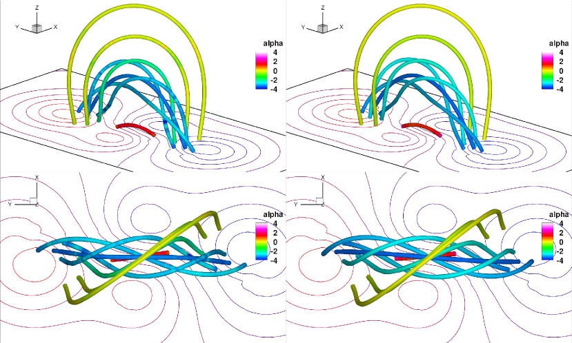
Figure 3: Selected field lines for The High_HFT case: left are the reference model and right the extrapolation. Contour lines on the bottom are plotted for $B_{z}$. The field lines are color-coded by the value of force-free factor $\alpha$.

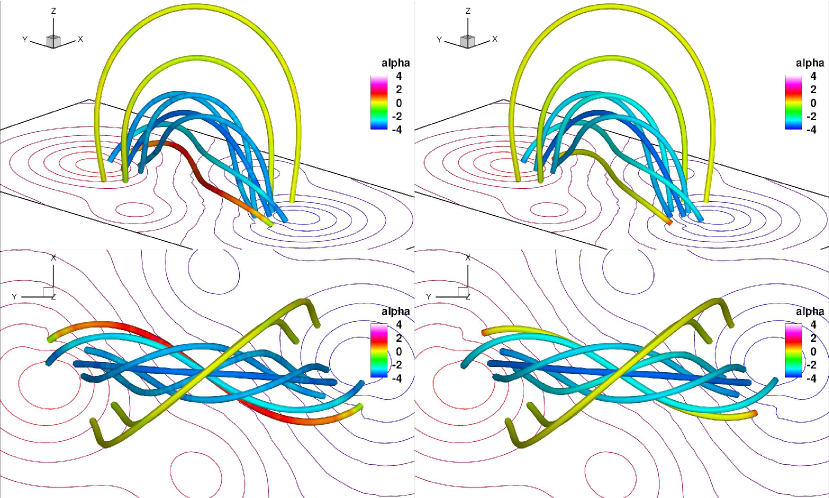
Figure 4: Selected field lines for The No_HFT case. The format is the same as Figure 3.

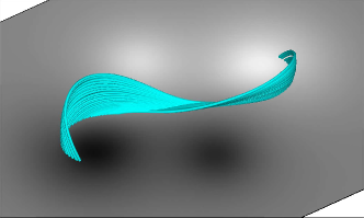
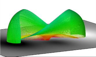
Figure 5: The reconstructed BPSS (left) and HFT (right) illustrated with continuous set of field lines (colors of the lines are used for a good visualization of the structures). They characterize the interface layers that separating the flux rope from its ambient field.