On pore–scale modeling and simulation of reactive transport in 3D geometries

Abstract

Pore–scale modeling and simulation of reactive flow in porous media has a range of diverse applications, and poses a number of research challenges. It is known that the morphology of a porous medium has significant influence on the local flow rate, which can have a substantial impact on the rate of chemical reactions. While there are a large number of papers and software tools dedicated to simulating either fluid flow in 3D computerized tomography (CT) images or reactive flow using pore–network models, little attention to date has been focused on the pore–scale simulation of sorptive transport in 3D CT images, which is the specific focus of this paper. Here we first present an algorithm for the simulation of such reactive flows directly on images, which is implemented in a sophisticated software package. We then use this software to present numerical results in two resolved geometries, illustrating the importance of pore–scale simulation and the flexibility of our software package.

1 Introduction

Understanding and controlling reactive flow in porous media is important for a number of environmental and industrial applications, including oil recovery, fluid filtration and purification, combustion and hydrology. Traditionally, the majority of theoretical and experimental research into transport within porous media has been carried out at macroscopic (Darcy) scale. Despite the progress in developing devices to perform experimental measurements at the pore–scale, experimental characterization of the pore–scale velocity, pressure and solute fields is still a challenging task. Due the influence of the pore–scale geometry on the processes of interest, direct numerical simulation (DNS) promises to be a very useful computational tool in a wide range of fields, and in combination with experimental studies, can be used to determine quantities of interest that are not experimentally quantifiable (Blunt et al., 2013).

Significant progress over the past 10 – 15 years in the pore–scale simulation of single phase flow has resulted in the computation of permeability tensors for natural and technical porous media becoming a standard procedure. A number of academic as well as commercial software tools, capable of processing 3D CT images in addition to virtually generating porous media, are available, for example Aviso, GeoDict and Ingrain. Most of those software tools have the additional ability of simulating two–phase immiscible flow at the pore–scale directly on a computational domain obtained through the segmentation of 3D CT images, often using the lattice Boltzmann (LB), the level set or volume of fluid methods. In contrast, substantially less work on the DNS of reactive flow has been performed, and only a few software tools with this capability exist. A limited number of computational studies examining reactive transport where the reactions only occur within the fluid phase (and not at a surface) exist (Molins et al., 2012; Shen et al., 2011). In contrast, the literature and computational tools examining full 3D reactive flow where the reactions occur at the pore wall (surface reactions), is sparse. The majority of existing studies and available numerical simulation packages describing pore–scale sorptive transport are based on pore–network mathematical models (see, for example, Raoof et al. (2010); Varloteaux et al. (2013) and literature therein), where the geometry needs to be converted into an idealized series of connected pores and throats to represent the porous medium. However, during this process, information on the morphology of the underlying media can be lost (see, for example, Raoof et al. (2010) and Lichtner and Kang (2007)). In this paper we present an algorithm and a sophisticated software package, called Pore–Chem, which uses cell centered finite volume (FV) methods to numerically solve 3D solute transport with surface reactions at the pore–scale. In particular the software package has the ability to solve the systems of equations modeling colloidal reactive transport on a geometrical domain obtained directly through imaging techniques, such as computerized tomography, which allows for a very accurate spatial description of the computational domain.

In this paper we describe the transport of a generic solute through the Navier–Stokes (NS) system of equations coupled to a convection–diffusion (CD) equation. The CD equation is complemented by boundary conditions which describe various types of surface reactions comprising a Robin boundary condition for the solute coupled to an ordinary differential equation (ODE) describing the dynamics of the adsorption at the pore wall. To represent the computational domain, a voxelized geometry is considered, where each individual voxel is either solid or fluid. The solute transport model is chosen due to its applicability to a broad range of problems. In addition, our goal is to describe the transport and reaction of sub–micron particles, for which inertial effects of the individual particles are negligible. Discrete models, where each particle is modeled as an individual entity, are necessary when considering larger particles, for example with a radius greater than one micron, for which inertial effects become important. Several commercial software packages, for example GeoDict (GeoDict, 2012–, 2014), solve a range of discrete mathematical models describing colloid transport and adsorption. However, numerical simulation of these models is often significantly more computationally expensive than a continuous mathematical model and accounting for different reaction kinetics is usually not possible in such packages.

Reactive flow in porous media is intrinsically a multiscale problem. The goal of our developments is to support problems where scale separation is possible and in cases where it is not possible. The first case, where the separation of scales is viable, is usually the focus of asymptotic homogenization theory. In the second case, when scale separation is not possible, numerical upscaling methods like multiscale finite element methods are often applied. During the homogenization procedure, when applicable, certain assumptions are imposed, allowing for the derivation of macroscopic (Darcy scale) equations from the microscale formulation, with effective parameters, such as the permeability and the effective reaction rate, obtained through solution of a cell problem (Hornung, 1997). A number of studies have employed homogenization theory to derive a macroscopic description of sorptive reactive transport for particular parameter regimes. The homogenization of solute transport in porous media in the presence of surface reactions has been performed for both high Péclet numbers (convection dominated regime) (Allaire et al., 2010b, a; Allaire and Hutridurga, 2012), and when the Péclet number is of order one (Hornung, 1994; Kumar et al., 2013; van Duijn, 1991). In addition to being able to solve cell problems in a number of settings, our software has the ability of solving a much broader class of problems at the pore–scale, without being restricted by the assumptions required during homogenization. Furthermore, it provides the possibility to study various different types of surface reactions described by different kinetics.

The remainder of the paper is organized as follows. In Section 2 the mathematical model is presented and cast into dimensionless variables. The method of achieving a numerical solution to the system of equations is outlined in Section 3, and illustrative results using this method are presented in Section 4. Finally, conclusions are drawn in Section 5.

2 Mathematical model

We now detail the mathematical model, which describes the transport and reaction of a generic solute at a 2D interface within a 3D pore–scale resolved geometry, where we assume that the number of solute particles is sufficiently large that representation within a continuum framework is valid.

Let us denote the spatial domain of interest by $\Omega$, an open subset of $\mathbb{R}^{3}$. We assume that we can decompose $\Omega$ into a solid domain, denoted by $\Omega_{s}$, and a fluid domain, denoted by $\Omega_{f}$, such that $\Omega=\Omega_{s}\cup\Omega_{f}$. Denoting the external boundary of our domain, being the closure of $\Omega$, by $\partial\Omega$, we partition this into an inlet, $\partial\Omega_{\text{in}}$, an outlet, $\partial\Omega_{\text{out}}$, and external walls, $\partial\Omega_{\text{wall}}$, so that

$$\partial\Omega=\partial\Omega_{\text{in}}\cup\partial\Omega_{\text{out}}\cup\partial\Omega_{\text{wall}}.$$ (1)

We note that, although we here consider only one inlet and one outlet, extension to consider multiple inlets and outlets is straightforward. Finally, we denote the interfacial boundary between the fluid and solid portions of the domain by $\Gamma=\Omega_{f}\cap\Omega_{s}$. To allow for different types of reactive boundary conditions to be described, we decompose $\Gamma$ into $N\geq 1$ different boundary types as follows

$$\Gamma=\cup_{i=0}^{N-1}\Gamma_{i},$$ (2)

where $\Gamma_{i}$ has distinct properties. Making such a decomposition enables us to attribute different reaction rates or kinetic descriptions to different portions of the domain, allowing for different types of solid material.

In order to describe the flow of the water through the membrane, by appealing to the conservation of momentum, the incompressible NS equations are used:

$$\rho\left(\displaystyle\frac{\partial\mathbf{v}}{\partial t}+\mathbf{v}\cdot\nabla\mathbf{v}\right) =-\nabla p+\mu\nabla\cdot\left(\nabla\mathbf{v}\right),$$ (3a)

$$\nabla\cdot\mathbf{v} =0,$$ (3b)

where $\mathbf{v}(\mathbf{x},t)$ and $p(\mathbf{x},t)$ are the velocity and pressure of the fluid respectively, while $\mu\geq 0$ and $\rho\geq 0$ are the viscosity and the density of the fluid which we assume are constants (Bear, 1988; Acheson, 1995). Suitable boundary conditions on $\partial\Omega$ are given by

$$\mathbf{v} =\textbf{V}_{\text{in}},\qquad \mathbf{x} \in\partial\Omega_{\text{in}},$$ (4a)

$$p =P_{\text{out}}\qquad \mathbf{x} \in\partial\Omega_{\text{out}},~{}$$ (4b)

$$\mathbf{v} =\mathbf{0},\qquad \mathbf{x} \in\partial\Omega_{\text{wall}},$$ (4c)

where $\textbf{V}_{\text{in}}$ is the inlet velocity with $\|\mathbf{V}_{\text{in}}\|>0$, $P_{\text{out}}$ is the pressure at the outlet, and $\mathbf{n}$ is the outward pointing normal to the boundary $\partial\Omega$. Although here we have used no–slip and no–flux flow conditions for the external walls, symmetry or periodic boundary conditions can also be imposed which may be more appropriate depending on the problem to be solved. Further boundary conditions are required to be specified on the reminder of the boundary to $\Omega_{f}$, being the fluid–solid interface. To allow for the slip of flow along the fluid–solid interface, and the inclusion of additional effects such as charged fluids or matrices, we use the Navier–Maxwell slip conditions, given by

$$\mathbf{v}\cdot\mathbf{n}=0,\qquad\mathbf{v}\cdot\mathbf{t}=\beta_{i}\mathbf{n}\cdot\left(\nabla\mathbf{v}+\left(\nabla\mathbf{v}\right)^{\mathrm{T}}\right)\cdot\mathbf{t},\qquad\mathbf{x}\in\Gamma_{i},\>t>0,$$ (5)

where $\beta_{i}$ is the slip length on $\mathbf{x}\in\Gamma_{i}$ for $i=0,1,\ldots N-1$ measured per unit length, $\mathbf{t}$ is any unit tangent to the surface such that $\mathbf{t}\cdot\mathbf{n}=0$, and the superscript $\mathrm{T}$ denotes the transpose (Lauga et al., 2007). In the case that $\beta_{i}=0$ for some $i$, then the standard no–slip and no–flux boundary conditions for the flow are enforced on $\Gamma_{i}$. We specify initial conditions through

$$\mathbf{v}(\mathbf{x},0)=\mathbf{v}_{0}(\mathbf{x}),\qquad p(\mathbf{x},0)=p_{0}(\mathbf{x}),\qquad\mathbf{x}\in\Omega_{f},$$ (6)

where $\mathbf{v}_{0}$ and $p_{0}$ are known functions. We discuss the choice for these in Section 3.

We denote the concentration of the solute within the fluid by $c(\mathbf{x},t)$, measured in particle number per unit volume. Appealing to the conservation of mass and assuming no fluid–phase reactions occur, the spatio–temporal evolution of the solute concentration is given by

$$\frac{\partial c}{\partial t}+\nabla\cdot\left(\mathbf{v}c\right)=D\nabla\cdot\left(\nabla c\right),\qquad\mathbf{x}\in\Omega_{f},t>0,$$ (7)

where $D\geq 0$ is the solute diffusion coefficient which we assume to be scalar and constant. We assume a known concentration of the solute at the inlet, and prescribe zero flux of the solute at the outlet and on the external walls as follows:

$$c =c_{\text{in}},\qquad \mathbf{x} \in\partial\Omega_{\text{in}},$$ (8a)

$$\nabla c\cdot\mathbf{n} =0,\qquad \mathbf{x} \in\partial\Omega_{\text{out}}\cup\partial\Omega_{\text{wall}},$$ (8b)

where $c_{\text{in}}>0$ is assumed to be constant.

2.1 Models for surface reactions

We are required to specify boundary conditions for $c(\mathbf{x},t)$ on $\mathbf{x}\in\Gamma_{i}$, to describe the surface reactions occurring here. In general, there are two stages of adsorption of a particle from the bulk solution to the solid surface. The first stage involves the diffusion of particles from the bulk solution to the subsurface and the second stage then involves the transfer of particles from the subsurface to the surface. After the adsorption of a molecule at the interface, there is a reorientation of the colloid molecules at the surface, which results in a change in the surface tension (Kralchevsky et al., 2008). Assuming that both the rate of diffusion of the particle from the bulk to the subsurface, and the rate of the transfer of the particles from the subsurface to the surface are important in determining the overall rate of reaction, we use a mixed kinetic–diffusion adsorption description, given by

$$-D\nabla c\cdot\mathbf{n}=\frac{\partial m}{\partial t}=f_{i}(c,m),\qquad\mathbf{x}\in\Gamma_{i}.\>t>0,$$ (9)

Here $m(\mathbf{x},t)$ is the surface concentration of the particle under consideration (Kralchevsky et al., 2008), measured in units of number per unit surface area, which contrasts with $c(\mathbf{x},t)$ being measured in units of number per unit volume. The function $f_{i}(c,m)$ describes the kinetics of the rate of change of the surface concentration on the $i^{\text{th}}$ reactive boundary for $i=0,\ldots N-1$ (Danov et al., 2002). Equation (9) states that the change in the surface concentration is equal to the flux across the surface, where the movement from the bulk to the surface is termed adsorption, and movement from the surface to the bulk is termed desorption. If $\Gamma_{i}$ is nonreactive, for some $i$, then $f_{i}=0$, so the adsorbed concentration on this boundary type remains constant, and a no–flux boundary condition for the solute concentration is prescribed. For reactive boundaries, the choice of $f_{i}$ and its dependence on $c$ and $m$ is highly influential in correctly describing the reaction dynamics at the solid–fluid interface. A number of different isotherms exist for describing these dynamics, dependent on the solute attributes, the order of the reaction, and the interface type.

The simplest of these is the Henry isotherm, which assumes a linear relationship between the surface pressure and the number of adsorbed particles, and takes the form

$$f_{i}=\kappa_{a,i}c-\kappa_{d,i}m,\qquad\mathbf{x}\in\Gamma_{i},\>t>0.$$ (10)

Here $\kappa_{a,i}\geq 0$ is the rate of adsorption, measured in unit length per unit time, and $\kappa_{d,i}\geq 0$ is the rate of desorption, measured per unit time, at reactive boundary type $i$ for $i=0,\ldots N-1$. Equation (10) states that the rate of adsorption is proportional to the concentration of particles in solution at the reactive surface. As such, the rate of adsorption predicted does not saturate at higher surface concentrations. However, physically we expect the rate of adsorption to decrease as the quantity of adsorbed particles increases and the available surface area for adsorption decreases. Even though the Henry isotherm predicts no limit to surface concentration and does not model any interaction between the particles, it has been used in a large number of analytical studies due to its linearity.

The Langmuir adsorption isotherm was the first to be derived mathematically, and is suitable to describe the adsorption of a monolayer of localized non–ionic non–interacting molecules at a 2D solid interface, and a derivation from statistical physics may be found in (Baret, 1969). It is also frequently used to describe the adsorption of molecules at a solid–liquid interface, and is described by

$$f_{i}=\kappa_{a,i}c\left(1-\frac{m}{m_{\infty,i}}\right)-\kappa_{d,i}m,\qquad\mathbf{x}\in\Gamma_{i},\>t>0.$$ (11)

Here $m_{\infty,i}>0$ is the maximal possible adsorbed surface concentration, measured in number per unit area, at reactive boundary type $i$ for $i=0,\ldots N-1$. In comparison to the Henry isotherm, the Langmuir isotherm predicts a decrease in the rate of adsorption as the adsorbed concentration increases due to the reduction in available adsorption surface. The Henry isotherm, given in Equation (10), is a linearization of Equation (11), explaining why it produces an accurate representation only at low surface concentrations.

More complex descriptions of the reaction kinetics exist to describe non–localized adsorption and particles which interact. For example, the Frumkin isotherm describes localized adsorption where particle interaction is accounted through an additional parameter:

$$f_{i}=\kappa_{a,i}c\left(1-\frac{m}{m_{\infty,i}}\right)-\kappa_{d,i}m\exp\left(-\displaystyle\frac{2\beta m}{kT}\right),\qquad\mathbf{x}\in\Gamma_{i},\>t>0.$$ (12)

where $k$ is the Boltzmann constant and $T$ is the temperature in Kelvin. The parameter $\beta\geq 0$ describes how cooperative the reaction is, and is related to the interaction energy between the particles. In the case that $\beta=0$, the Langmuir isotherm is recovered. The Frumkin isotherm is infrequently used in the mathematical modeling of colloidal transport, which may be due its nonlinearity and the difficulties in determining the interaction energy between the particles.

We make the assumption that the adsorption or desorption of our solute does not alter the position of the reactive boundary, which in the case of small volumes of particles being adsorbed is sufficiently accurate. By the conservation of mass, such an assumption implies any adsorption or desorption on the surface is represented by a corresponding increase or decrease in the density of the solid material through time. In some cases, for example when the molecules are big or the number being adsorbed is large, interface evolution needs to be considered and may be done in a similar manner to Tartakovsky et al. (2008); Roubinet and Tartakovsky (2013) and Boso and Battiato (2013). This is particularly important in the application of rock dissolution and precipitation, where large geometrical changes are observed.

To close the system of equations, we impose the initial conditions

$$c(\mathbf{x},0)=c_{0}(\mathbf{x}),\qquad\mathbf{x}\in\Omega_{f},\qquad m(\mathbf{x},0)=m_{0,i}(\mathbf{x}),\quad\mathbf{x}\in\Gamma_{i},$$ (13)

where $c_{0}$ and $m_{0,i}$ are known for $i=0,1,\ldots N-1$.

Our problem is, therefore, described by two systems of equations with one–way coupling; the incompressible NS equations, described by (3) – (6) and the CD equation described by (7) – (8), with reactive boundaries conditions (9), initial conditions (13), and a description of the reaction kinetics, for example Equation (10), (11) or (12). We now cast the equations into dimensionless variables, before detailing the methods used to obtain a numerical solution.

2.2 Nondimensionalization

Using a caret notation to distinguish the dimensionless variable from its dimensional equivalent, we let

$$\mathbf{x}=L\hat{\mathbf{x}},\quad\mathbf{v}=V_{\text{in}}\hat{\mathbf{v}},\quad t=\frac{L\hat{t}}{V_{\text{in}}},\quad p=P_{\text{out}}+\rho V_{\text{in}}^{2}\hat{p},\quad c=c_{\text{in}}\hat{c},\quad m=c_{\text{in}}L\hat{m},\quad M=c_{\text{in}}L^{3}\hat{M},$$

where $L>0$ is a typical length scale of the computational domain and $V_{\text{in}}=\|\mathbf{V}_{\text{in}}\|$. As our computational domain consists of voxels, the relationship between each voxel and its material property is conserved upon nondimensionalization, while the length, area and volume of each voxel scales with $L$, $L^{2}$ and $L^{3}$ respectively. Given this, we let $\hat{\Omega}$, $\hat{\Omega}_{s}$ and $\hat{\Omega}_{f}$, with boundaries $\partial\hat{\Omega}_{\text{in}}$, $\partial\hat{\Omega}_{\text{out}}$, $\partial\hat{\Omega}_{\text{wall}}$ and $\hat{\Gamma}_{i}$ for $i=0,1,\ldots N-1$ represent the dimensionless versions of the equivalent dimensional domains and boundaries, where the voxel size is scaled accordingly. In dimensionless variables, we, therefore, have

$$\left(\displaystyle\frac{\partial\hat{\mathbf{v}}}{\partial\hat{t}}+\hat{\mathbf{v}}\cdot\hat{\nabla}\hat{\mathbf{v}}\right) =-\hat{\nabla}\hat{p}+\frac{1}{\mathrm{Re}}\hat{\nabla}^{2}\hat{\mathbf{v}},$$ (14a)

$$\hat{\nabla}\cdot\hat{\mathbf{v}} =0,$$ (14b)

$$\frac{\partial\hat{c}}{\partial\hat{t}}+\hat{\nabla}\cdot\left(\hat{\mathbf{v}}\hat{c}\right) =\frac{1}{\mathrm{Pe}}\hat{\nabla}\cdot\left(\hat{\nabla}\hat{c}\right),$$ (14c)

where

$$\mathrm{Re}=\displaystyle\frac{L\rho V_{\text{in}}}{\mu},\qquad\mathrm{Pe}=\displaystyle\frac{V_{\text{in}}L}{D},$$ (15)

are the global Reynolds and Péclet numbers respectively, being the ratio between the inertial and viscous forces and the ratio between advective and diffusive transport rates respectively. Boundary conditions are given by

$$\hat{\mathbf{v}} =\mathbf{n},\qquad \hat{\mathbf{x}} \in\partial\hat{\Omega}_{\text{in}},$$ (16a)

$$\hat{p} =0\text{ and }\hat{\nabla}\hat{\mathbf{v}}\cdot\mathbf{n}=\mathbf{0}\qquad \hat{\mathbf{x}} \in\partial\hat{\Omega}_{\text{out}},$$ (16b)

$$\hat{\mathbf{v}} =\mathbf{0},\qquad \hat{\mathbf{x}} \in\partial\hat{\Omega}_{\text{wall}},$$ (16c)

$$\hat{\mathbf{v}}\cdot\mathbf{n} =0,\text{ and }\hat{\mathbf{v}}\cdot\mathbf{t}=\hat{\beta}_{i}\mathbf{n}\cdot\left(\hat{\nabla}\hat{\mathbf{v}}+\left(\hat{\nabla}\hat{\mathbf{v}}\right)^{\mathrm{T}}\right)\cdot\mathbf{t},\qquad \hat{\mathbf{x}} \in\hat{\Gamma}_{i},$$ (16d)

$$\frac{1}{\mathrm{Pe}}\hat{\nabla}\hat{c}\cdot\mathbf{n} =\frac{\partial\hat{m}}{\partial\hat{t}}=\hat{f}_{i}(\hat{c},\hat{m}),\qquad \hat{\mathbf{x}} \in\hat{\Gamma}_{i},$$ (16e)

$$\hat{c} =1,\qquad \hat{\mathbf{x}} \in\partial\hat{\Omega}_{\text{in}},$$ (16f)

$$\hat{\nabla}\hat{c}\cdot\mathbf{n} =0,\qquad \hat{\mathbf{x}} \in\partial\hat{\Omega}_{\text{out}}\cup\partial\hat{\Omega}_{\text{wall}},$$ (16g)

with $\hat{\beta}_{i}=\displaystyle\frac{\beta_{i}}{L}$. In the case of the Henry isotherm, we have

$$\hat{f}_{i}=\mathrm{Da}^{\textrm{I}}_{a,i}\hat{c}-\mathrm{Da}^{\textrm{I}}_{d,i}\hat{m},\qquad\hat{\mathbf{x}}\in\hat{\Gamma}_{i},\>\hat{t}>0,$$ (17)

whereas, nondimensionalization of the Langmuir and Frumkin isotherms yields

$$\hat{f}_{i}=\mathrm{Da}^{\textrm{I}}_{a,i}\hat{c}\left(1-\frac{\hat{m}}{\hat{m}_{\infty,i}}\right)-\mathrm{Da}^{\textrm{I}}_{d,i}\hat{m},\qquad\hat{\mathbf{x}}\in\hat{\Gamma}_{i},\>\hat{t}>0,$$ (18)

and

$$\hat{f}_{i}=\mathrm{Da}^{\textrm{I}}_{a,i}\hat{c}\left(1-\frac{\hat{m}}{\hat{m}_{\infty,i}}\right)-\mathrm{Da}^{\textrm{I}}_{d,i}\hat{m}\exp\left(-\hat{\beta}\hat{m}\right),\qquad\hat{\mathbf{x}}\in\hat{\Gamma}_{i},\>\hat{t}>0,$$ (19)

respectively, for $i=0,1,\ldots N-1$, where $\hat{\beta}=\displaystyle\frac{2\beta c_{\text{in}}L}{kT}$ and $\hat{m}_{\infty,i}=\displaystyle\frac{m_{\infty,i}}{c_{\text{in}}L}$. In (17) – (19) the Damköhler numbers are given by

$$\mathrm{Da}_{a,i}=\displaystyle\frac{\kappa_{a,i}}{V_{\text{in}}},\qquad\text{and}\qquad\mathrm{Da}_{d,i}=\displaystyle\frac{\kappa_{d,i}L}{V_{\text{in}}},$$ (20)

and describe, for each $i$, the ratio of the rate of reaction (either adsorptive or desorptive) to the rate of advective transport. The initial conditions are given by

$$\hat{\mathbf{v}}(\hat{\mathbf{x}},0) =\hat{\mathbf{v}}_{0}(\hat{\mathbf{x}}),\qquad\hat{p}(\hat{\mathbf{x}},0)=\hat{p}_{0}(\hat{\mathbf{x}}),\quad\hat{c}(\hat{\mathbf{x}},0)=\hat{c}_{0}(\hat{\mathbf{x}}), \hat{\mathbf{x}}\in\hat{\Omega}_{f},$$ (21a)

$$\hat{m}(\hat{\mathbf{x}},0) =\hat{m}_{0,i}(\hat{\mathbf{x}}), \hat{\mathbf{x}}\in\hat{\Gamma}_{i},$$ (21b)

where $\hat{\mathbf{v}}_{0}(\hat{\mathbf{x}})=\displaystyle\frac{\mathbf{v}_{0}(\mathbf{x})}{V_{\text{in}}}$, $\hat{p}_{0}(\hat{\mathbf{x}})=\displaystyle\frac{p_{0}(\mathbf{x})-P_{\text{out}}}{\rho V_{\text{in}}^{2}}$, $\hat{c}_{0}(\hat{\mathbf{x}})=\displaystyle\frac{c_{0}(\mathbf{x})}{c_{\text{in}}}$ and $\hat{m}_{0,i}(\hat{\mathbf{x}})=\displaystyle\frac{m_{0,i}(\mathbf{x})}{c_{\text{in}}L}$ for $i=0,1,\ldots N-1$.

We now proceed to discuss the numerical methods used to obtain an approximate solution to our dimensionless system of equations given by (14), with boundary conditions given by (16) – (18) and initial conditions specified through (21).

3 Numerical methods

The full system of equations cannot be solved using analytical techniques, and so numerical methods need to be employed to calculate an approximate solution. We employ FV methods to numerically solve our system of equations, motivated by their local mass conserving properties. Other methods, for example LB or finite difference methods may also be used for solving the flow problem. We note that our CD solver is completely compatible with LB methods (the compatibility of our solver with finite difference methods depends on the grid selection). Although the authors are not aware of a detailed comparison of the performance of FV and LB methods in solving the NS equations at the pore–scale, some incomplete internal studies indicate that LB methods can be advantageous for geometries with a very low porosity and a high tortuosity, while FV methods are favorable in other cases.

Due to the one–way coupling between our two systems of equation, the velocity and pressure solutions are at steady state. For the sake of generality, we consider the unsteady equations, and begin by solving the system of equations describing the fluid flow, namely (14a), (14b) along with (16a) – (16d), to obtain a steady state numerical solution where $\displaystyle\frac{\partial\hat{\mathbf{v}}}{\partial\hat{t}}=\mathbf{0}$ is satisfied. This is achieved using a Chorin fractional timestepping method and we refer the reader to Čiegis et al. (2007) and Lakdawala (2010) for full details and for further references, where the methods used are described.

Once the solution of $\hat{\mathbf{v}}$ is obtained, we proceed to solve the system of equations describing the solute transport and reaction, (14c) along with the boundary conditions (16e) – (18) and initial conditions (21), using a FV method with a cell-centered grid. For the sake of brevity, full details of the numerical method employed are not given, but we refer the reader to, for example Causon et al. (2011), for more detailed information on FV methods. Firstly, dimensionless time is uniformly partitioned into $Q$ time points, denoted by $\hat{t}^{0},\hat{t}^{1},\ldots\hat{t}^{Q-1}$ with $\hat{t}^{k}=k\left(\Delta\hat{t}\right)$, where $\Delta\hat{t}$ is the dimensionless timestep size. Then the spatial domain, $\hat{\Omega}$, is split into $P$ non–overlapping cubic finite volumes, $\mathcal{B}_{l}$ for $l=0,1,\ldots P_{1}$, which span the 3D computational domain, such that $\hat{\Omega}=\cup_{l=0}^{P-1}\mathcal{B}_{l}$. Considering a single representative finite volume, $\mathcal{B}_{l}$, we denote its six faces by $\mathcal{F}_{l,j}$ with center $\hat{\mathbf{x}}_{j}$ where the subscript $j=e,w,n,s,t,b$ denotes the east, west, north, south, top and bottom faces respectively. Integration of (14c) over the control volume, $\mathcal{B}_{l}$, and time interval $[\hat{t}^{k},\hat{t}^{k+1}]$, upon application of the divergence theorem, yields

$$\int_{\mathcal{B}_{l}}\hat{c}(\hat{\mathbf{x}},\hat{t}^{k+1})\>\mathrm{d}V-\int_{\mathcal{B}_{l}}\hat{c}(\hat{\mathbf{x}},\hat{t}^{k})\>\mathrm{d}V+\int_{\hat{t}^{k}}^{\hat{t}^{k+1}}\int_{\partial\mathcal{B}_{l}}\hat{\mathbf{v}}\hat{c}\cdot\mathbf{n}\>\mathrm{d}S\>\mathrm{d}\tau=\frac{1}{\mathrm{Pe}}\int_{\hat{t}^{k}}^{\hat{t}^{k+1}}\int_{\partial\mathcal{B}_{l}}\hat{\nabla}\hat{c}\cdot\mathbf{n}\>\mathrm{d}V\>\mathrm{d}\tau,$$

where $\partial\mathcal{B}_{l}$ is the boundary of $\mathcal{B}_{l}$, so that $\partial\mathcal{B}_{l}=\sum_{j=e,w,n,s,t,b}\mathcal{F}_{l,j}$ . Denoting the center of the finite volume by $\mathbf{x}_{c}$ and using the approximations $\displaystyle\int_{\mathcal{F}_{l,j}}\phi(\hat{\mathbf{x}},\hat{t})\>\mathrm{d}S=\hat{A}_{j}\phi(\hat{\mathbf{x}}_{j},\hat{t})$ and $\displaystyle\int_{\mathcal{B}_{l}}\phi(\hat{\mathbf{x}},\hat{t})\>\mathrm{d}S=|\mathcal{B}_{l}|\phi(\hat{\mathbf{x}}_{c},\hat{t})$, for some scalar function $\phi$ for $j=n,s,e,w,t,b$, where $\hat{A}_{j}$ is the area of the face $\mathcal{F}_{l,j}$, we have

$$|\mathcal{B}_{l}|\left(\hat{c}(\hat{\mathbf{x}}_{c},\hat{t}^{k+1})-\hat{c}(\hat{\mathbf{x}}_{c},\hat{t}^{k})\right)\\ +\int_{\hat{t}^{k}}^{\hat{t}^{k+1}}\left(\hat{A}_{e}\left[\hat{\mathbf{v}}\hat{c}\right]_{\hat{\mathbf{x}}_{e}}-\hat{A}_{w}\left[\hat{\mathbf{v}}\hat{c}\right]_{\hat{\mathbf{x}}_{x}}+\hat{A}_{n}\left[\hat{\mathbf{v}}\hat{c}\right]_{\hat{\mathbf{x}}_{n}}-\hat{A}_{s}\left[\hat{\mathbf{v}}\hat{c}\right]_{\hat{\mathbf{x}}_{s}}+\hat{A}_{t}\left[\hat{\mathbf{v}}\hat{c}\right]_{\hat{\mathbf{x}}_{t}}-\hat{A}_{b}\left[\hat{\mathbf{v}}\hat{c}\right]_{\hat{\mathbf{x}}_{b}}\right)\>\mathrm{d}\tau\\ =\frac{1}{\mathrm{Pe}}\int_{\hat{t}^{k}}^{\hat{t}^{k+1}}\left(\hat{A}_{e}\left[\frac{\partial\hat{c}}{\partial\hat{x}}\right]_{\hat{\mathbf{x}}_{e}}-\hat{A}_{w}\left[\frac{\partial\hat{c}}{\partial\hat{x}}\right]_{\hat{\mathbf{x}}_{w}}+\hat{A}_{n}\left[\frac{\partial\hat{c}}{\partial\hat{y}}\right]_{\hat{\mathbf{x}}_{n}}-\hat{A}_{s}\left[\frac{\partial\hat{c}}{\partial\hat{y}}\right]_{\hat{\mathbf{x}}_{s}}+\hat{A}_{t}\left[\frac{\partial\hat{c}}{\partial\hat{z}}\right]_{\hat{\mathbf{x}}_{t}}-\hat{A}_{b}\left[\frac{\partial\hat{c}}{\partial\hat{z}}\right]_{\hat{\mathbf{x}}_{b}}\right)\>\mathrm{d}\tau.$$

Denoting $\hat{c}_{j}(\tau)=\hat{c}(\hat{\mathbf{x}}_{j},\tau)$ and $\hat{\mathbf{v}}_{j}(\tau)=\hat{\mathbf{v}}(\hat{\mathbf{x}}_{j},\tau)$ for $j=n,s,e,w,t,b,c$, by first order finite difference methods we have

$$|\mathcal{B}_{l}|\left(\hat{c}_{c}(\hat{t}^{k+1})-\hat{c}_{c}(\hat{t}^{k})\right)+\int_{\hat{t}^{k}}^{\hat{t}^{k+1}}\hat{A}_{e}\hat{\mathbf{v}}_{e}\hat{c}_{e}-\hat{A}_{w}\hat{\mathbf{v}}_{w}\hat{c}_{w}+\hat{A}_{n}\hat{\mathbf{v}}_{n}\hat{c}_{n}-\hat{A}_{s}\hat{\mathbf{v}}_{s}\hat{c}_{s}+\hat{A}_{t}\hat{\mathbf{v}}_{t}\hat{c}_{t}-\hat{A}_{b}\hat{\mathbf{v}}_{b}\hat{c}_{b}\>\mathrm{d}\tau\\ =\int_{\hat{t}^{k}}^{\hat{t}^{k+1}}\frac{2}{\mathrm{Pe}}\left(\hat{A}_{e}\frac{\hat{c}_{e}-\hat{c}_{c}}{\delta\hat{x}}-\hat{A}_{w}\frac{\hat{c}_{c}-\hat{c}_{w}}{\delta\hat{x}}+\hat{A}_{n}\frac{\hat{c}_{n}-\hat{c}_{c}}{\delta\hat{y}}-\hat{A}_{s}\frac{\hat{c}_{c}-\hat{c}_{s}}{\delta\hat{y}}+\hat{A}_{t}\frac{\hat{c}_{t}-\hat{c}_{c}}{\delta\hat{z}}-\hat{A}_{b}\frac{\hat{c}_{c}-\hat{c}_{b}}{\delta\hat{z}}\right)\>\mathrm{d}\tau,$$ (22)

where $\delta\hat{x}$, $\delta\hat{y}$ and $\delta\hat{z}$ are the width, length and height of the control volume $\mathcal{B}_{l}$. By virtue of using voxelized geometry, we know that $\delta\hat{x}=\delta\hat{y}=\delta\hat{z}$, $\hat{A}_{j}=\left(\delta\hat{x}\right)^{2}$ for all $j=n,s,e,w,t,b$, and $|\mathcal{B}_{l}|=\left(\delta\hat{x}\right)^{3}$. By the implicit Euler method, we, therefore, have

$$\frac{\delta\hat{x}\left(\hat{c}_{c}^{k+1}-\hat{c}_{c}^{k}\right)}{\Delta\hat{t}}+\hat{\mathbf{v}}_{e}^{k+1}\hat{c}_{e}^{k+1}-\hat{\mathbf{v}}_{w}\hat{c}_{w}^{k+1}+\hat{\mathbf{v}}_{n}^{k+1}\hat{c}_{n}^{k+1}-\hat{\mathbf{v}}_{s}^{k+1}\hat{c}_{s}^{k+1}+\hat{\mathbf{v}}_{t}^{k+1}\hat{c}_{t}^{k+1}-\hat{\mathbf{v}}_{b}^{k+1}\hat{c}_{b}^{k+1}\\ =\frac{2}{\mathrm{Pe}\>\delta\hat{x}}\left(\hat{c}_{e}^{k+1}+\hat{c}_{w}^{k+1}+\hat{c}_{n}^{k+1}+\hat{c}_{s}^{k+1}+\hat{c}_{t}^{k+1}+\hat{c}_{b}^{k+1}-6\hat{c}_{c}^{k+1}\right),$$ (23)

where $\hat{c}_{j}^{k}=\hat{c}(\hat{\mathbf{x}}_{j},\hat{t}^{k})$ for $j=n,s,e,w,t,b,c$. In the case that one of the faces of the control volume lies on a boundary, the appropriate boundary conditions must be discretized; for the inlet, outlet and solid (or symmetry) boundaries this is straightforward due to the Dirichlet and zero Neumann boundary condition imposed there via (16f) and (16g). Therefore, we omit the details for the discretization of the boundary conditions on the external boundary $\partial\hat{\Omega}$. The appropriate discretization of the reactive boundary conditions, prescribed on the fluid–solid interface through (16e) and the corresponding description of the reaction kinetics, here either (17), (18) or (19), is slightly more involved and deserves a more detailed discussion.

In a fully implicit and coupled discretization the resulting discrete equations are nonlinear and the Newton method needs to be used (Kelley, 1995). In a broad class of practically interesting problems we have considered to date, we have not faced very strong coupling between the dissolved and adsorbed concentrations. Therefore, a fully implicit and coupled discretization was not required and we have found that an operator splitting approach, or just a Picard linearization, has worked well. In this approach, the dissolved particle concentration is computed at $\hat{t}=\hat{t}^{k+1/2}$, and then the value is used to compute the deposited mass at the time $\hat{t}=\hat{t}^{k+1}$. Runge–Kutta methods, or other methods for numerically solving stiff ODEs, are also straightforward to implement, and may be the subject of future studies if required (Kelley, 1995). In order to illustrate the method used in Pore–Chem, we describe the discretization for the Langmuir isotherm, which is achieved as follows. Firstly (18) is substituted into (16e), which is then split into a Robin boundary condition and an ordinary differential equation:

$$-\frac{1}{\mathrm{Pe}}\hat{\nabla}\hat{c}\cdot\mathbf{n} =\mathrm{Da}^{\textrm{I}}_{a,i}\hat{c}\left(1-\frac{\hat{m}}{\hat{m}_{\infty,i}}\right)-\mathrm{Da}^{\textrm{I}}_{d,i}\hat{m},$$ (24a)

$$\frac{\partial\hat{m}}{\partial\hat{t}} =\mathrm{Da}^{\textrm{I}}_{a,i}\hat{c}\left(1-\frac{\hat{m}}{\hat{m}_{\infty,i}}\right)-\mathrm{Da}^{\textrm{I}}_{d,i}\hat{m}.$$ (24b)

If $\mathrm{Da}^{\textrm{I}}_{a,i}\displaystyle\frac{\hat{c}}{\hat{m}_{\infty,i}}+\mathrm{Da}^{\textrm{I}}_{d,i}=0$, then either $\hat{c}=\mathrm{Da}^{\textrm{I}}_{d,i}=0$ or $\mathrm{Da}^{\textrm{I}}_{a,i}=\mathrm{Da}^{\textrm{I}}_{d,i}=0$. In both of these cases, by (18), $\hat{f}_{i}=0$ and so no reactions occur at the spatiotemporal point under consideration, in which case, by (24a), we have $\hat{\nabla}\hat{c}\cdot\mathbf{n}=0$ and a zero Neumann boundary condition, which is straightforward to implement. Otherwise, if $\mathrm{Da}^{\textrm{I}}_{a,i}\displaystyle\frac{\hat{c}}{\hat{m}_{\infty,i}}+\mathrm{Da}^{\textrm{I}}_{d,i}>0$, assuming that $\hat{c}(\hat{\mathbf{x}},\hat{t})$ is constant over the time period in question, namely $\hat{t}\in[\hat{t}^{k},\hat{t}^{k+1}]$, and equal to $\hat{c}(\hat{\mathbf{x}})$ at each spatial point, (24b) may be integrated to give

$$\hat{m}(\hat{\mathbf{x}},\hat{t}^{k+1})=\frac{\mathrm{Da}^{\textrm{I}}_{a,i}\hat{c}(\hat{\mathbf{x}})-B\exp\left(-\left(\mathrm{Da}^{\textrm{I}}_{a,i}\hat{c}(\hat{\mathbf{x}})\hat{m}_{\infty,i}^{-1}+\mathrm{Da}^{\textrm{I}}_{d,i}\right)\hat{t}^{k+1}\right)}{\mathrm{Da}^{\textrm{I}}_{a,i}\hat{c}(\hat{\mathbf{x}})\hat{m}_{\infty,i}^{-1}+\mathrm{Da}^{\textrm{I}}_{d,i}},\qquad\hat{\mathbf{x}}\in\hat{\Gamma}_{i},\>\hat{t}>0.$$ (25)

Here $B$ is a constant of integration which may be evaluated at $\hat{t}=\hat{t}^{k}$ to give

$$B=\left(\mathrm{Da}^{\textrm{I}}_{a,i}\hat{c}(\hat{\mathbf{x}})\left(1-\hat{m}(\hat{\mathbf{x}},\hat{t}^{k})\hat{m}_{\infty,i}^{-1}\right)-\mathrm{Da}^{\textrm{I}}_{d,i}\hat{m}(\hat{\mathbf{x}},\hat{t}^{k})\right)\exp\left(\left(\mathrm{Da}^{\textrm{I}}_{a,i}\hat{c}(\hat{\mathbf{x}})\hat{m}_{\infty,i}^{-1}+\mathrm{Da}^{\textrm{I}}_{d,i}\right)\hat{t}^{k}\right).$$ (26)

Upon substitution into (25), we have

$$\hat{m}(\hat{\mathbf{x}},\hat{t}^{k+1})\\ =\frac{\mathrm{Da}^{\textrm{I}}_{a,i}\hat{c}(\hat{\mathbf{x}},\hat{t}^{k})-\left(\mathrm{Da}^{\textrm{I}}_{a,i}\hat{c}(\hat{\mathbf{x}},\hat{t}^{k})\left(1-\hat{m}(\hat{\mathbf{x}},\hat{t}^{k})\hat{m}_{\infty,i}^{-1}\right)-\mathrm{Da}^{\textrm{I}}_{d,i}\hat{m}(\hat{\mathbf{x}},\hat{t}^{k})\right)\exp\left(-\left(\mathrm{Da}^{\textrm{I}}_{a,i}c(\hat{\mathbf{x}},\hat{t}^{k})\hat{m}_{\infty,i}^{-1}+\mathrm{Da}^{\textrm{I}}_{d,i}\right)(\Delta\hat{t})\right)}{\mathrm{Da}^{\textrm{I}}_{a,i}\hat{c}(\hat{\mathbf{x}},\hat{t}^{k})\hat{m}_{\infty,i}^{-1}+\mathrm{Da}^{\textrm{I}}_{d,i}},$$ (27)

for $\hat{\mathbf{x}}\in\hat{\Gamma}_{i}$, $\hat{t}>0$, where we have approximated $\hat{c}(\hat{\mathbf{x}})$ by $\hat{c}(\hat{\mathbf{x}},\hat{t}^{k})$. This is done to prevent nonlinear terms in unknown variables from appearing in the discretized version of (16e). Discretization of the other two isotherms is implemented in a similar manner.

Consequently, we may approximate the Robin boundary condition, (16e), on the reactive face $\mathcal{F}_{l,j}\in\hat{\Gamma}_{i}$ for $j=e,w,n,s,t,b$ and $i=0,1,\ldots N-1$ using finite difference methods fully implicitly as follows:

$$-\left(\frac{2n}{\mathrm{Pe}\>\delta\hat{x}}+\mathrm{Da}^{\textrm{I}}_{a,i}\right)c_{j}^{k+1}+2n\frac{c_{c}^{k+1}}{\mathrm{Pe}\>\delta\hat{x}}\\ =-\left(\frac{\mathrm{Da}^{\textrm{I}}_{a,i}}{\hat{m}_{\infty,i}}+\mathrm{Da}^{\textrm{I}}_{d,i}\right)\left(\frac{\mathrm{Da}^{\textrm{I}}_{a,i}\hat{m}_{j}^{k}-\left(\mathrm{Da}^{\textrm{I}}_{a,i}c_{j}^{k}\left(1-\hat{m}_{j}^{k}\hat{m}_{\infty,i}^{-1}\right)-\mathrm{Da}^{\textrm{I}}_{d,i}\hat{m}_{j}^{k}\right)\exp\left(-\left(\mathrm{Da}^{\textrm{I}}_{a,i}c_{m}^{p}\hat{m}_{\infty,i}^{-1}+\mathrm{Da}^{\textrm{I}}_{d,i}\right)(\Delta t)\right)}{\mathrm{Da}^{\textrm{I}}_{a,i}c_{j}^{k}\hat{m}_{\infty,i}^{-1}+\mathrm{Da}^{\textrm{I}}_{d,i}}\right),$$ (28)

where $n=\pm 1$ is the direction of the outward pointing normal. Using (28), the appropriate terms are assembled, along with (23) minus the relevant diffusive flux term, for the finite volume on which the reactive surface lies into a matrix $\mathcal{A}^{k+1}$ and vector $\mathbf{g}^{k+1}$, where $\mathcal{A}^{k+1}\hat{\mathbf{c}}^{k+1}=\mathbf{g}^{k+1}$ and $\hat{\mathbf{c}}^{k+1}$ is a vector of the dimensionless solutions $\hat{c}(\hat{\mathbf{x}},\hat{t}^{k+1})$ at the discretized points of the computational domain. Once all the terms for all the finite volumes within the domain have been assembled into $\mathcal{A}^{k+1}$ and $\mathbf{g}^{k+1}$, the equation $\mathcal{A}^{k+1}\hat{\mathbf{c}}^{k+1}=\mathbf{g}^{k+1}$ is solved using a biconjugate gradient stabilized method to give the updated fluid concentration, $\hat{c}^{k+1}$, at each discrete spatial point in $\hat{\Omega}_{f}$, while the updated adsorbed concentration, $\hat{m}^{k+1}$, is given by (26). Time is then updated, the next timestep considered, and we proceed in the usual manner until the final time point is reached.

Figure 1: Flow chart to illustrate how numerical computation of the transport with surface reactions is implemented within Pore–Chem, with main features indicated only. The light red ovals indicate input files, while the yellow ovals indicate output files. The green and the blue rectangular boxes indicate steps involved for the flow and efficiency solvers respectively, while the dark red boxes indicate steps involved in both. The white diamonds indicate decision making steps. In the case that the dimensional system of equations is being solved, the appropriate dimensionless quantities of interest are replaced by the dimensional equivalent.

Numerical simulation of the equations is performed in Pore–Chem and a schematic, outlining the numerical algorithm used, is given in Figure 1. In the following section, the dimensionless equations are solved, but we present results in dimensional quantities.

4 Results

We present illustrative results, using the numerical method outlined in Section 3, on two separate computational domains, a real geometry and a virtually generated geometry, for two applications where surface reactions are important. The first set of simulations are performed on a portion of palatine sandstone, obtained using micro computerized tomography ($\mu$–CT) by Frieder Enzmann at the Johannes Gutenberg University of Mainz (Becker et al., 2011). Surface reactions are highly important in many fields of the Earth sciences, including calcite growth, oxidation–reduction reactions, formation of biofilms, to name only a few (Steefel et al., 2005). The second set of results is performed on a computational domain virtually constructed to be representative of a commercially available microfiltration functionalized membrane. The use of functionalized membranes is a promising method for removing contaminants from water, and involves treating the pore walls of the membrane so that they adsorb certain microorganisms or drugs (Ulbricht, 2006). Such membranes have pore sizes on the sub–micron scale and the resolution provided by $\mu$–CT imaging techniques is not high enough to give representative images, motivating the use of a virtually generated geometry. The two computational domains under consideration are shown in Figure 2.

(a) Rock geometry

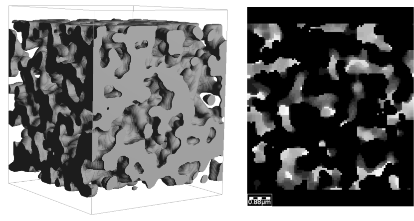
(b) Membrane geometry

Figure 2: The two computational domains under consideration, plotted in 3D on the left–hand side of the figure, and in 2D through a representative cross section on the right–hand side of the figure. Figure 2(a) shows the palatine sandstone geometry obtained through $\mu$–CT, with a voxel size of $1.4\times 10^{-6}$ $\mathrm{m}$, as used in Becker et al. (2011). Figure 2(b) shows a virtually generated geometry which aims to reproduce the morphology of a commercially available microfiltration membrane, with a voxel length of $7.03\times 10^{-8}$ $\mathrm{m}$ (3 s.f.) This geometry was created using the software GeoDict (GeoDict, 2012–, 2014), and a comparison to experimentally evaluated quantities is made in Di Nicolò et al. (2015).

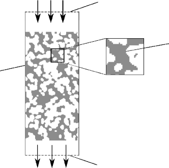
Figure 3: Schematic to illustrate the computational domain. The solid microfiltration membrane is show in grey while the water is shown in white. Voxels are added to the top and bottom of the domain, at the inlet and outlet, to enable free–flow to develop. Modified, with permission, from Di Nicolò et al. (2015).

For the numerical simulations presented, a dead–end setup is used, with a schematic illustrating the domain and boundary conditions shown in Figure 3. Layers of pure water voxels are added at the inlet and at the outlet, as shown in Figure 2 and illustrated in Figure 3, to allow free flow to develop. This results in a total computational domain size of $200\times 200\times 300$ voxels for the sandstone geometry, and $100\times 100\times 120$ voxels for the membrane geometry. For the results presented one type of reactive solid–fluid interface is considered, so that $N=1$, and consequently we now drop the $i$ subscript notation relating to the type of reactive boundary.

4.1 Fluid flow

As described in Section 3, we are first required to solve for the fluid flow. We assume that the fluid generates no slip as it passes over the membrane, and we set the slip length, $\beta$, to be zero so that, by (5), there is zero normal and tangential velocity at the fluid–solid interface, $\Gamma$. We set inflow velocities to be typical for the application under consideration, and use $V_{\text{in}}=1$ $\mathrm{mm}/\mathrm{s}$ for the membrane geometry and $V_{\text{in}}=1.5\times 10^{-4}$ $\mathrm{mm}/\mathrm{s}$ for the rock geometry. The parameters chosen for the inlet velocities, and the fluid density and viscosity, yield small Reynolds numbers; $\mathrm{Re}=4.2\times 10^{-7}$ in the case of the rock geometry and $\mathrm{Re}=7.83\times 10^{-3}$ for the membrane geometry. Therefore, the fluid flow in both computational domains is in a Stokes regime. Solving (14a) and (14b), along with the boundary conditions (16a) – (16d), numerically until steady–state is achieved, yields the solutions as reproduced in Figure 4. Due to our assumption that the maximal possible number of adsorbed particles is sufficiently small to ignore the effects of geometry modification, these remain constant through time. Examination of Figure 4 reveals the dependence of the local velocity field on the morphology of the computational domains.

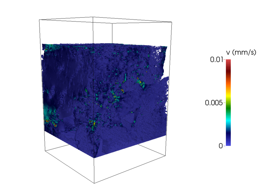
(a) Velocity magnitude, rock

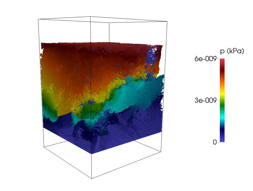
(b) Pressure, rock

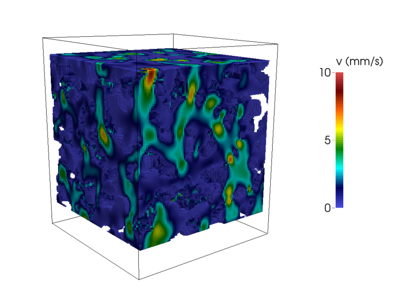
(c) Velocity magnitude, membrane

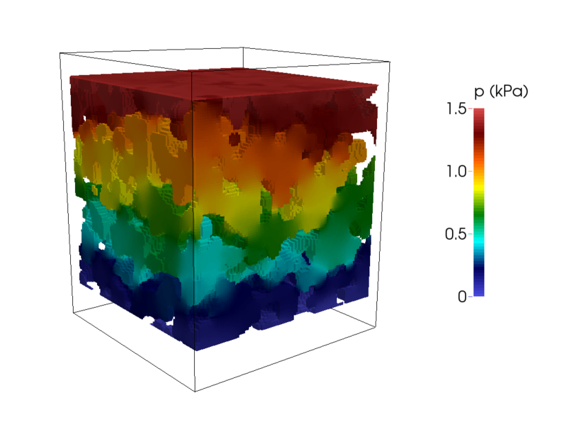
(d) Pressure, membrane

Figure 4: Velocity magnitude, 4(a) and 4(c), and pressure, 4(b) and 4(d), fields, measured in $\mathrm{mm}/\mathrm{s}$ and $\mathrm{kPa}$ respectively for both the computational domains considered. Due to our assumption that the adsorption of the solute does not alter the geometry, these remain constant throughout the experimental time frame. The black boxes shows the outline for the entire computational domain, where we exclude the additional voxels embedded at the inlet and the outlet for 3D plotting purposes.

4.2 Contaminant transport

We now turn our attention to solving the reactive flow. Illustrative parameters are used, and we employ the Henry isotherm, given by Equation (10), for the rock geometry, and the Langmuir isotherm, given by Equation (11), for the membrane geometry. We choose $c_{\text{in}}$ arbitrarily to be $2\times 10^{4}$ $\mathrm{number}/\mathrm{mm}^{3}$ and we set the initial concentration of fluid contaminant to be equal to the inflow boundary condition, so that $\hat{c}_{0}(\hat{\mathbf{x}})=1$ for $\hat{\mathbf{x}}\in\hat{\Omega}_{f}$, while the quantity of adsorbed contaminant is initially assumed to be zero, $\hat{m}_{0}(\mathbf{x})=0$. Furthermore, for the membrane geometry, we set the dimensionless maximal surface concentration of adsorbed contaminant, $\hat{m}_{\infty}$, to be $10^{-4}$, which equates to a dimensional value of $m_{\infty}=0.014$ $\mathrm{number}/\mathrm{mm}^{2}$. Due to the form of the equations, the choice of $c_{\text{in}}$ does not influence the dimensionless system of equations describing the transport and reaction of the contaminant given by (14c) along with the boundary conditions (16e) – (19), except for through the parameter $\hat{m}_{\infty}$. Therefore, increasing or decreasing $c_{\text{in}}$ for fixed $\hat{m}_{\infty}$ purely scales the dimensional concentration (both fluid and adsorbed) by a constant factor.

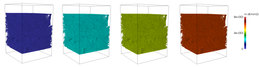
Figure 5: The retained concentration of contaminant, $m$, for the rock geometry at 1200 second time intervals where $\mathrm{Da}_{a}=0.1$, $\mathrm{Da}_{d}=0.001$ and $\mathrm{Pe}=2.0\times 10^{-5}$. The fluid concentration remains effectively constant throughout the domain and so this is not plotted.

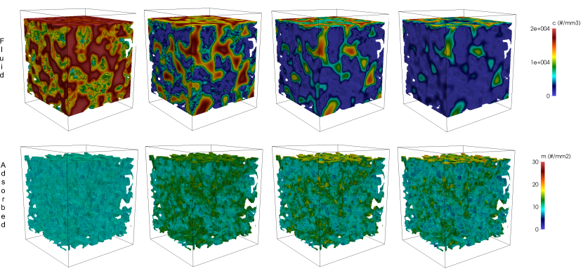
Figure 6: Numerical results at $5\times 10^{-5}$ $\mathrm{s}$ intervals for the fluid concentration, $c$, and the adsorbed concentration, $m$, of contaminant in the membrane geometry.

Figure 5 illustrates the concentration of the contaminant on the solid surface over time for the rock geometry, where we use $\mathrm{Da}_{a}=0.1$, $\mathrm{Da}_{d}=0.001$ and $\mathrm{Pe}=2.0\times 10^{-5}$. Due to the slow rate of reaction and small Péclet number, the quantity of solute adsorbed over this time period is not large enough to significantly alter the fluid concentration over the time period under consideration. Furthermore, as the rate of reaction is much smaller than the mass transport rate, the adsorbed concentration remains spatially homogeneous.

In contrast, with the parameters $\mathrm{Pe}=10$ and $\mathrm{Da}_{a}=\mathrm{Da}_{d}=10$ for the membrane geometry, we see significant spatial heterogeneity in both the dissolved and adsorbed concentrations, as illustrated in Figure 6. As time progresses, the fast rates of reaction result in a depletion of the dissolved concentration at the pore wall and a dependence of both the dissolved and adsorbed concentrations on the local membrane morphology.

5 Conclusions

We have presented an algorithm for solving solute transport at the pore–scale within a resolved porous medium, with reversible surface adsorption at the pore wall. A pore–scale description of reactive transport, as opposed to a description at the Darcy scale, allows for a very accurate representation of the processes of interest. The system of equations comprise the NS equations and a CD equation, with Robin boundary conditions coupled to an ODE accounting for the surface reactions. Assuming that each particle is sufficiently small in size not to alter the flow of the fluid within the computational domain, and that its reaction at the wall does not significantly alter the pore–scale geometry, there is a one–way coupling between the NS and CD systems of equations. Although, for simplicity, we consider one species of solute and examine only surface reactions, extension to several different species of solute with both volumetric and surface reactions is straight forward and implemented within our software package Pore–Chem. The algorithm presented employs a FV method, and in this paper we have particularly focused on the discretization method used to solve the reactive boundary conditions for the adsorption and desorption at the interface. Illustrative numerical results, using our software package Pore–Chem, are presented on two separate geometries. The first of these is a 3D $\mu$–CT image of a piece of Palatine Sandstone rock, while the second geometry is virtually generated within GeoDict (GeoDict, 2012–, 2014) to be representative of a commercially available functionalized membrane. The results demonstrate the potential of such a numerical package, with the ability to solve reactive transport directly on images and on virtually generated geometries, in further progressing the understanding of the interplay between the transport and reaction rates at the pore–scale. In a future publication, currently in preparation, we will investigate the influence of the computational domain morphology on the reaction dynamics, and investigate the effect of different parameter regimes on the numerical results and quantities of interest.

The advantages of using a pore–scale description are multiple. Firstly, it allows us to simulate reactive transport over a range of different parameter regimes, and in particular, outside the applicability region of the equivalent upscaled model. In highly disordered media the Péclet number can significantly vary locally, which poses problems for asymptotic upscaling methods, but not for a pore–scale description. Secondly, different kinetic models for the reactions can be used without the need to re–perform the upscaling procedure. In the future we plan to extend the algorithm in order to solve coupled multiscale problems using the heterogeneous multiscale method, in a similar manner to Battiato et al. (2011) and Iliev et al. (2014). Such a development will enable problems at larger spatial scales to be considered, which could aid further research into the influence of pore–scale processes in a number of highly interesting and important research applications.

References

- Acheson (1995) D.J. Acheson. Elementary Fluid Dynamics. Oxford applied mathematics and computing science series. Clarendon Press, 1995.
- Allaire and Hutridurga (2012) G. Allaire and H. Hutridurga. Homogenization of reactive flows in porous media and competition between bulk and surface diffusion. IMA Journal of Applied Mathematics, 77(6):788–815, 2012. doi: 10.1093/imamat/hxs049.
- Allaire et al. (2010a) G. Allaire, R. Brizzi, A. Mikelić, and A. Piatnitski. Two-scale expansion with drift approach to the Taylor dispersion for reactive transport through porous media. Chemical Engineering Science, 65(7):2292–2300, April 2010a. doi: 10.1016/j.ces.2009.09.010.
- Allaire et al. (2010b) G. Allaire, A Mikelić, and A Piatnitski. Homogenization approach to the dispersion theory for reactive transport through porous media. Society of Industrial and Applied Mathematics Journal on Mathematical Analysis, 42(1):125–144, 2010b. doi: 10.1137/090754935.
- Baret (1969) J. F. Baret. Theoretical model for an interface allowing a kinetic study of adsorption. Journal of Colloid and Interface Science, 30(1):1–12, 1969.
- Battiato et al. (2011) I. Battiato, D. M. Tartakovsky, A. M. Tartakovsky, and T. D. Scheibe. Hybrid models of reactive transport in porous and fractured media. Advances in Water Resources, 34(9):1140–1150, September 2011. doi: 10.1016/j.advwatres.2011.01.012.
- Bear (1988) J. Bear. Dynamics of Fluids in Porous Media. Dover Civil and Mechanical Engineering Series. Dover, 1988. ISBN 9780486656755.
- Becker et al. (2011) J. Becker, E. Glatt, and A. Wiegmann. Combining pore morphology and flow simulations to determine two-phase properties of 3d tomograms. Extended Abstract for Flows and mechanics in natural porous media from pore to field scale, Pore2Filed, IFP Energies nouvelles, 2011.
- Blunt et al. (2013) M. J. Blunt, B. Bijeljic, H. Dong, O. Gharbi, S. Iglauer, P. Mostaghimi, A. Paluszny, and C. Pentland. Pore-scale imaging and modelling. Advances in Water Resources, 51:197–216, January 2013. doi: 10.1016/j.advwatres.2012.03.003.
- Boso and Battiato (2013) F. Boso and I. Battiato. Homogenizability conditions for multicomponent reactive transport. Advances in Water Resources, 62:254–265, 2013. doi: 10.1016/j.advwatres.2013.07.014.
- Causon et al. (2011) P. D. M. Causon, P. C. G. Mingham, and L. Qian. Introductory Finite Volume Methods for PDEs. Bookboon, 2011. ISBN 9788776818821.
- Danov et al. (2002) K. D. Danov, D. S. Valkovska, and P. A. Kralchevsky. Adsorption relaxation for nonionic surfactants under mixed barrier-diffusion and micellization-diffusion control. Journal of Colloid and Interface Science, 251(1):18–25, 2002.
- Di Nicolò et al. (2015) E. Di Nicolò, O. Iliev, and K. Leonard. Virtual generation of microfiltration membrane geometry for the numerical simulation of contaminent transport. Technical Report 245, Fraunhofer-Institut für Techno- und Wirtschaftsmathematik ITWM, 2015.
- GeoDict, 2012– (2014) GeoDict, 2012–2014. The virtual material laboratory GeoDict. http://www.geodict.com, 2012 – 2014.
- Hornung (1994) Jäger W. Mikelić A. Hornung, U. Reactive transport through an array of cells with semi-permeable membranes. ESAIM: Mathematical Modelling and Numerical Analysis - Modélisation Mathématique et Analyse Numérique, 28(1):59–94, 1994.
- Hornung (1997) U. Hornung. Homogenization and Porous Media. Interdisciplinary Applied Mathematics. Springer New York, 1997. ISBN 9780387947860.
- Iliev et al. (2014) O. Iliev, Z. Lakdawala, and G. Printsypar. On a multiscale approach for filter efficiency simulations. Computers & Mathematics with Applications, 67(12):2171–2184, 2014. doi: 10.1016/j.camwa.2014.02.022.
- Kelley (1995) C. T. Kelley. Iterative Methods for Linear and Nonlinear Equations, volume 16 of Frontiers in applied mathematics. Society of Industrial and Applied Mathematics, 1995.
- Kralchevsky et al. (2008) P. A. Kralchevsky, K. D. Danov, and N. D. Denkov. Handbook of Surface and Colloid Chemistry, Third Edition, chapter Chemical Physics of Colloid Systems and Interfaces. Taylor & Francis, 2008. ISBN 9781420007206.
- Kumar et al. (2013) K. Kumar, I. S. Pop, and F. Radu. Numerical analysis for an upscaled model for dissolution and precipitation in porous media. Numerical Mathematics and Advanced Applications, pages 703–711, 2013.
- Lakdawala (2010) Z. Lakdawala. On Efficient Algorithms for Filtration Related Multiscale Problems. PhD thesis, University of Kaiserslautern, 2010.
- Lauga et al. (2007) E. Lauga, M. Brenner, and H. Stone. Microfluidics: The No-Slip Boundary Condition. In C. Tropea, A. L. Yarin, and J. F. Foss, editors, Springer Handbook of Experimental Fluid Mechanics, pages 1219–1240. Springer Berlin Heidelberg, 2007.
- Lichtner and Kang (2007) P. C. Lichtner and Q. Kang. Upscaling pore-scale reactive transport equations using a multiscale continuum formulation. Water Resources Research, 43(12):W12S15+, 2007. doi: 10.1029/2006wr005664.
- Molins et al. (2012) S. Molins, D. Trebotich, C. I. Steefel, and C. Shen. An investigation of the effect of pore scale flow on average geochemical reaction rates using direct numerical simulation. Water Resources Research, 48(3):W03527, 2012. doi: 10.1029/2011wr011404.
- Raoof et al. (2010) A. Raoof, S. M. Hassanizadeh, and A. Leijnse. Upscaling transport of adsorbing solutes in porous media: Pore–network modeling. Vadose Zone Journal, 9:624–636, 2010. doi: 10.2136/vzj2010.0026.
- Roubinet and Tartakovsky (2013) D. Roubinet and D. M. Tartakovsky. Hybrid modeling of heterogeneous geochemical reactions in fractured porous media. Water Resources Research, 49(12):7945–7956, 2013. doi: 10.1002/2013wr013999.
- Shen et al. (2011) C. Shen, D. Trebotich, S. Molins, D. T. Graves, B. Van Straalen, T. Ligocki, and C. I. Steefel. High performance computations of subsurface reactive transport processes at the pore scale. In Proceedings of Scientific Discovery through Advanced Computing, 2011. URL https://seesar.lbl.gov/anag/publications/treb/SciDAC2011_sim.pdf.
- Steefel et al. (2005) C. Steefel, D. Depaolo, and P. Lichtner. Reactive transport modeling: An essential tool and a new research approach for the Earth sciences. Earth and Planetary Science Letters, 240(3-4):539–558, 2005. doi: 10.1016/j.epsl.2005.09.017.
- Tartakovsky et al. (2008) A. M. Tartakovsky, D. M. Tartakovsky, T. D. Scheibe, and P. Meakin. Hybrid Simulations of Reaction-Diffusion Systems in Porous Media. Society for Industrial Applied Mathematics Journal on Scientific Computing, 30(6):2799–2816, January 2008.
- Ulbricht (2006) M. Ulbricht. Advanced functional polymer membranes. Polymer, 47(7):2217–2262, 2006. doi: 10.1016/j.polymer.2006.01.084.
- van Duijn (1991) Knabner P. van Duijn, C. J. Solute transport in porous media with equilibrium and non-equilibrium multiple-site adsorption: Travelling waves. J. reine angewandte Math, 415:1–49, 1991.
- Varloteaux et al. (2013) C Varloteaux, M. T. Vu, S. Békri, and P. M. Adler. Reactive transport in porous media: pore-network model approach compared to pore-scale model. Physical Review E: Statistical, Nonlinear, and Soft Matter Physics, 87(2), 2013. doi: http://dx.doi.org/10.1103/PhysRevE.87.023010.
- Čiegis et al. (2007) R. Čiegis, O. Iliev, and Z. Lakdawala. On parallel numerical algorithms for simulating industrial filtration problems. Computational Methods in Applied Mathematics, 7:118–134, 2007. doi: 10.2478/cmam-2007-0007.