Abstract

Many approaches to transform classification problems from non-linear to linear by feature transformation have been recently presented in the literature. These notably include sparse coding methods and deep neural networks. However, many of these approaches require the repeated application of a learning process upon the presentation of unseen data input vectors, or else involve the use of large numbers of parameters and hyper-parameters, which must be chosen through cross-validation, thus increasing running time dramatically. In this paper, we propose and experimentally investigate a new approach for the purpose of overcoming limitations of both kinds. The proposed approach makes use of a linear auto-associative network (called SCNN) with just one hidden layer. The combination of this architecture with a specific error function to be minimized enables one to learn a linear encoder computing a sparse code which turns out to be as similar as possible to the sparse coding that one obtains by re-training the neural network. Importantly, the linearity of SCNN and the choice of the error function allow one to achieve reduced running time in the learning phase. The proposed architecture is evaluated on the basis of two standard machine learning tasks. Its performances are compared with those of recently proposed non-linear auto-associative neural networks. The overall results suggest that linear encoders can be profitably used to obtain sparse data representations in the context of machine learning problems, provided that an appropriate error function is used during the learning phase.

1 Introduction

Various approaches to transform classification problems from non-linear to linear by a feature transformation have been recently investigated. These notably include sparse coding methods [1, 2, 3, 4, 5] and deep neural networks [6, 7]. However, two remarkable limitations usually affect these approaches: (i) most of the current sparse coding methods [1, 3, 4, 8, see, for example,] require the repeated application of some learning process in order to compute an input sparse representation, whenever the algorithm is fed with an input vector which was never used during the training phase; (ii) even though auto-associative neural networks enable one to overcome limitation (i), many of them, such as deep belief networks, present several levels of complexity or non-linearity. In fact, their learning methods usually involve a large number of parameters and hyper-parameters, such as the number of hidden units for more than one hidden layer, learning rates, momentum, weight decay, and so on. These parameters must be chosen through cross-validation, thus leading to a dramatic increase of running time. Interestingly, some authors [8, 9] suggest that simpler architectures, requiring a reduced number of parameters to be found, may enable one to achieve state-of-the-art performance. Following up this suggestion, the use of a relatively “simple” neural network approach, overcoming limitations (i) and (ii), is proposed here and experimentally investigated in terms of a trade-off between computational costs and performances.

The problem of overcoming limitations (i) and (ii) was addressed (a) by selecting an auto-associative neural network which enables one to learn a mapping between data and code space (the encoder) during the learning phase so that the learned mapping can be subsequently used on unseen data; and (b) by choosing just one linear hidden layer with identity as output function, jointly with an error function which allows one to learn at the same time both the encoder and the decoder by taking explicitly into account the contributions given by the two mappings. Given the linearity of the hidden layer and the selected error function, “good” learning rate parameters, ensuring linear rates of convergence in the minimization of error function, can be chosen in an explicit form without using cross-validation.

Points (a) and (b) guarantee that a reduced number of parameters must be determined during the learning phase: these are the number of hidden nodes and the sparsity parameter value which controls the extent to which the coding is sparse. On account of this fact, the present approach turns out to be computationally less expensive than deep neural networks and standard sparse coding approaches alike. Importantly, the present approach enables one to compute a linear encoder by means of which, during the test phase (on unseen data), one obtains a sparse code which is as similar as possible to the sparse code that one obtains by re-training the neural network. By applying a non-linear operation such as soft-thresholding or soft-max on this code one obtains a non-linear feature transformation. The rest of the paper is organized as follows.The selected auto-associative neural network and its relation to previously proposed approaches are discussed in Section 2 and 3, respectively. The experiment and its outcomes are presented in Section 4. In particular, in 4.1 tests showing the capability of our approach to reproduce PCA behaviour are described and discussed, whereas the ability to obtain appropriate sparse data representations enabling one to solve two standard machine learning tasks is evaluated in 4.2, 4.3.1 and 4.3.2. Our approach is additionally compared with two auto-associative neural networks recently proposed in literature ([10], [11] and with current results presented in the literature). Finally, Section 5 is devoted to an analysis of experimental results and their significance.

2 Background and related work

In the context of machine learning, the problem that we are considering here is usually expressed in terms of a minimization problem as follows:

$$min_{\mathbf{U},\mathbf{D}}\|\mathbf{X}-\mathbf{U}\mathbf{D}^{T}\|_{F}^{2}+\lambda\Omega(\mathbf{U})$$

$$\text{Subject to }\|D^{j}\|_{2}^{2}\leq 1,\forall j$$ (1)

where $\mathbf{X}$ is a $N\times p$ matrix containing the $N$ $p$-dimensional signals to be represented, $\mathbf{D}$ is a $p\times m$ matrix containing the basis vectors (or atoms) column-wise arranged, $\mathbf{U}$ is a $N\times m$ matrix containing the sparse representations of the signals in $\mathbf{X}$, $\Omega(\mathbf{U})$ is a norm or quasi-norm regularizing the solutions of the minimization problem, and the parameter $\lambda\geq 0$ controls to what extent the representations are regularized. The regularization term penalizes the solutions containing many coefficients that are different from zero.

Importantly, approaches of this kind give rise to a crucial limitation: after the learning phase, when an unseen data input vector $\mathbf{x}$ is considered, a minimization process is again required to compute its sparse representation $\mathbf{u}$. Sparse coding with auto-associative neural networks overcomes this limitation, and several approaches based on this observation have been accordingly proposed [12, 13, 7, 14, 15, see, for example, ].

In a nutshell, these approaches are based on an encoder-decoder architecture. The input $\mathbf{x}$ is fed into the encoder which produces a feature vector $\mathbf{u}$, i.e., a code of $\mathbf{x}$. In turn, the code $\mathbf{u}$ is fed as input into the decoder module which reconstructs the input $\mathbf{x}$ from the code. Both encoder and decoder are feed-forward neural networks which may present several degrees of non-linearity. The encoder and the decoder are trained so as to minimize the error between input $\mathbf{x}$ and reconstructed input, with the proviso that the code $\mathbf{u}$ must satisfy certain given constraints in order to obtain a sparse code of $\mathbf{x}$. Sometimes a further term is added in (1) so as to make the output of the encoder as similar as possible to the code $\mathbf{u}$ [2, 5, e.g.]. Such a term is added in our approach as well (see Section 3). Importantly, as mentioned in the previous section, some authors [8, 9] identified, as a drawback of many such architectures, their considerable complexity and computational cost. Notably, the learning processes involved in these approaches usually require a large number of hyper-parameters such as learning rates, momentum, weight decay, and so on, that must be chosen through cross-validation, thus increasing running times dramatically. Furthermore, it is possible to achieve state-of-the-art performance by means of simpler architectures requiring the identification of a reduced number of parameters.

Recently proposed architectures [10, 11], that we now turn to examine, involve non-linear auto-associative neural networks, called respectively ASCNN and SAANN, and a single hidden layer. Both networks, differently from our approach, can be used with a non-linear activation function $\varphi$ (e.g., sigmoid for SAANN and tanh for ASCNN) on the hidden layer units.

In SAANN the error function expressed in (2) is used. This function involves two terms. The first term is the standard reconstruction error between the input signals $\mathbf{X}$ and the reconstructed signals $\mathbf{U}\mathbf{D}^{T}$with $\mathbf{U}=\varphi(\mathbf{XC}^{T}$), where $\mathbf{C}$ (a.k.a. projection dictionary) is the weight matrix of the first weight layer of the network and $\mathbf{D}$ (a.k.a. reconstruction dictionary) is the weight matrix of the second weight layer of the network. The second term is a regularization term which imposes sparse codes of the input. As one may readily note from (2), the second term is a function of the hidden units’ output. Moreover the optimization algorithm simultaneously finds the reconstruction dictionary $\mathbf{D}$ and the projection dictionary $\mathbf{C}$ by a standard gradient descent technique.

$$E(\mbox{{D}},\mathbf{C})=\frac{1}{2}\|\mathbf{X}-\varphi(\mathbf{XC}^{T})\mathbf{D}^{T}\|_{F}^{2}+\lambda\sum_{n}\sum_{i}{log(1+u_{ni}{}^{2})}$$ (2)

In ASCNN the problems of finding the reconstruction and the projection dictionaries are addressed separately by dividing the autoassociative network into two subnetworks: top network, and bottom network. The optimization algorithm involves two basic steps:

1. Only the Bottom Network is considered. The input to the hidden units $\mathbf{Z}$ together with the reconstruction dictionary $\mathbf{D}$ are obtained by minimizing the following error function:
   

   $$E(\mathbf{Z},\mathbf{D})=\frac{1}{2}\|\mathbf{X}-\varphi(\mathbf{Z})\mathbf{D}^{T}\|_{F}^{2}+\lambda f\left(\frac{\mathbf{Z}}{\sigma}\right)$$ (3)

   
   

   an alternating optimizations technique is used to find $\mathbf{Z}$ and $\mathbf{D}$. The first term in equation (3) is the usual reconstruction error, the second term is a regularization term which imposes sparse solutions for the input codes. The sparseness function $f(\bullet)$ is chosen on the basis of the activation function $\varphi$ of the hidden units. A possible choice is $f(a)=log(1+a^{2})$ when the activation function corresponds either to $\tanh$ or to a linear function. $\lambda$ is a positive value which controls the relevance of the regularization term.

2. Only the Top Network is considered. The projection dictionary $\mathbf{C}$ is retrieved by minimizing the following error function with respect to :
   

   $$E(\mathbf{C})=\frac{1}{2}\|\mathbf{XC}^{T}-\mathbf{Z}\|_{F}^{2}$$ (4)

   leaving $\mathbf{Z}$ fixed.

Finally the whole autoassociative network is considered in order to achieve a fine tuning of network parameters ($\mathbf{Z}$, $\mathbf{C}$, and $\mathbf{D}$) by minimizing the error function (3) and by taking into account that $\mathbf{Z}=\mathbf{XC}^{T}$.

Both networks, ASCNN and SAANN, are trained by means of the mini batch stochastic gradient descent learning algorithm because the error function is differentiable as the penalization term is differentiable.

The possibility of identifying valid alternatives to non-linear approaches to sparse coding, in the context of non-linear autoassociative networks with a single hidden layer, is suggested by some classification which were successfully addressed on the basis of linear network approaches. Notably, linear approaches were successfully used to model the early stage responses of the visual system. In the early stage visual information is a small number of simultaneously active neurons among the much larger number of available neurons. The first attempt to model this behaviour of the visual system is due to Olshausen and Field ([16]). The authors built a simple single weight layer feed forward neural network (Sparsenet) where the observed data $\mathbf{X}$ are a linear combination of top-bottom basis vectors $\mathbf{D}$ and top-layer sparse responses $\mathbf{U}$. The sparsity of the solution is obtained by minimizing an error function composed of the standard sum-of-squares error and a regularization term, which can be expressed as follows:

$$E(\mathbf{D},\mathbf{U})=\frac{1}{2}\parallel\mathbf{X}-\mathbf{U}\mathbf{D}^{T}\parallel_{F}^{2}+\lambda\sum_{i=1}^{m}g\left(\frac{\mathbf{U}_{i}}{\sigma}\right)$$ (5)

where $g$ is a sparse inducing function, $\sigma$ is a scaling constant, and $\lambda$ is the usual positive value which controls the relevance of the regularization term.

3 Sparse Coding Neural Network: a linear approach

In order to investigate more systematically linear approaches, in the context of encoder-decoder architectures, we introduce here:

• an auto-associative network with linear activation functions only;

• an error function which allows one to learn at the same time both projection and reconstruction dictionaries by taking explicitly into account the contributions given by these two dictionaries; in particular, we introduce a term in the error function which enables one to obtain a sparse code which is as similar as possible to the output of the encoder.

• a hard sparse coding approach, i.e., a limited number of values different from zero, by means of a non-differentiable term in the error function. We use hard sparse coding also in view of the fact that it is an efficient representation of biological network behaviours ([17]).

Thus, we build a linear autoassociative neural network with two weight layers. From now on, this network will be called Sparse Coding Neural Network (SCNN). During the learning phase SCNN can be regarded as being formed by two independent sub-networks (see figure (1)): a top network, T-SCNN, which includes both the projection dictionary $\mathbf{C}$ and the SCNN hidden layer, and a bottom nework, B-SCNN, which includes both the reconstruction dictionary $\mathbf{D}$ and the SCNN output layer. In this phase, T-SCNN and B-SCNN are iteratively and successively trained. This training process is fundamentally based on two consecutive stages. First stage: both B-SCNN input signals,$\mathbf{U}$, and the reconstruction dictionary, $\mathbf{D}$, are learned by considering $\mathbf{X}$ as target values and by imposing a specific constraint on $\mathbf{U}$ to obtain sparse input signals. Second stage: the projection dictionary $\mathbf{C}$ is learned for T-SCNN by considering $\mathbf{X}$ as input values and $\mathbf{U}$ as target values. Consequently, SCNN is trained by minimizing the following global error function:

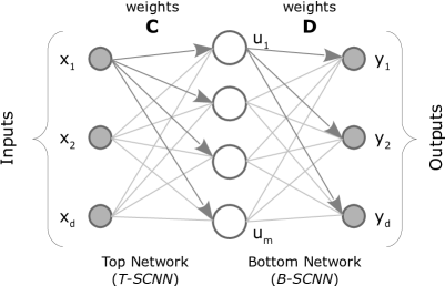
Figure 1: A graphical representation of the SCNN network. Top network (T-SCNN) includes both the projection dictionary $\mathbf{C}$ and the hidden layer. Bottom network (B-SCNN) includes both the reconstruction dictionary $\mathbf{D}$ and the SCNN output layer.

$$E(\mathbf{D},\mathbf{C},\mathbf{U})= \frac{1}{p}\sum\limits_{n=1}^{N}\sum\limits_{i=1}^{p}\left(x_{ni}-\sum\limits_{h=1}^{m}u_{nh}d_{ih}\right)^{2}+$$

$$\frac{1}{m}\sum\limits_{n=1}^{N}\sum\limits_{j=1}^{m}\left(u_{nj}-\sum\limits_{h=1}^{p}x_{nh}c_{jh}\right)^{2}+$$

$$\frac{2\lambda}{m}\sum\limits_{n=1}^{N}\sum\limits_{h=1}^{m}|u_{nh}|$$

$$\text{s.t.}\sum\limits_{h=1}^{p}\left(d_{hi}\right)^{2}\leq 1$$ (6)

where $x_{ni}$ is the $i$-th component of the $n$-th input signal, $u_{nh}$ is the $h$-th component of the input code when the network is fed with the $n$-th input signal, $d_{ih}$ is the weight associated to the connection going from the $h$-th hidden unit to the $i$-th output unit, and $c_{jh}$ is the weight associated to the connection going from the $h$-th input component to the $j$-th hidden unit. The first term forces the bottom network to reconstruct correctly the input signals $\mathbf{X}$ on the basis of both $\mathbf{U}$ and $\mathbf{D}$, the second term in (6) constrains the solutions of the minimization problem to obtain B-SCNN input ($u_{nj}$) as similar as possible to T-SCNN output ($\sum_{h=1}^{m}x_{nh}c_{jh}$), and the last term imposes a sparse representation for $\mathbf{U}$. Moreover, a quadratic constrain on the columns of $\mathbf{D}$ is imposed to avoid $\mathbf{U}$ being the null matrix.

Let us now describe in more detail the proposed learning approach. Since the error function ((6)) is separately convex in each variable, we proceed by iteratively minimizing with respect to B-SCNN input variables $u_{ni}$, while keeping unchanged both $d_{ij}$ and $c_{jk}$ (B-SCNN input update), then minimizing with respect to the reconstruction weights $d_{ij}$ while keeping unchanged both $u_{ni}$ and $c_{jk}$ (B-SCNN weight update) and, finally, minimizing with respect to the projection weights $c_{jk}$ while keeping unchanged both $d_{ij}$ and $u_{ni}$ (T-SCNN weight update). Importantly, the last term in (6) is not differentiable, and consequently it does not allow one to perform a classical gradient descent learning algorithm.

One can overcome this difficulty using proximal methods. Since the partial derivatives with respect to the weights $d_{ij}$ and $c_{jk}$ do not involve the non-differentiable term, these derivatives can be computed following the standard back-propagation approach:

$$\frac{\partial E}{\partial d_{ij}}=-\frac{2}{d}\sum_{n=1}^{N}u_{nj}\left(x_{ni}-\sum_{h=1}^{m}d_{ih}u_{nh}\right)$$ (7)

where $x_{ni}$ is taken as target for the bottom network , $d_{ih}$ is the weight from neuron $h$ to neuron $i$ of the bottom network, and $u_{nh}$ is $h$-th component of the $n$-th B-SCNN input vector.

$$\frac{\partial E}{\partial c_{jk}}=-\frac{2}{m}\sum_{n=1}^{N}x_{nk}\left(u_{nj}-\sum_{h=1}^{p}c_{jh}x_{nh}\right)$$ (8)

where $u_{nj}$ is the $j$-th component of the $n$-th B-SCNN’s input vector taken as target for the top network, $c_{jh}$ is the weight from neuron $h$ to neuron $j$ of the top network, and $x_{nh}$ is the $h$-th component of the $n$-th T-SCNN’s input vector .

Thus the update of the weights $d_{ij}$ and $c_{jk}$ is obtained on the basis of a standard gradient descend as follows:

$$d_{ij}^{s}=d_{ij}^{s-1}+\eta_{D}\frac{\partial E}{\partial d_{ij}}$$ (9)

$$c_{jk}^{s}=c_{jk}^{s-1}+\eta_{C}\frac{\partial E}{\partial c_{jk}}$$ (10)

where $s$ is the iteration step, and $\eta_{C}$, $\eta_{D}$ are the learning rates. Moreover, to fulfill the quadratic constrain in ((6)) a projection operator on the unit ball is applied on the columns of $\mathbf{D}$.

As mentioned above, since the last term in (6) is not differentiable, the update of $\mathbf{U}$ must be performed using a proximal algorithm. In summary, a proximal algorithm minimizes a function of type $E(\xi)=E_{1}(\xi)+E_{2}(\xi)$, where $E_{1}$ is convex and differentiable, with Lipschitz continuous gradient, while $E_{2}$ is lower semicontinuous, convex and coercive. These assumptions on $E_{1}$ and $E_{2}$ are necessary to ensure the existence of a solution. The proximal algorithm is given by combining a projection operator $(P)$ with a forward gradient descent step, as follows:

$$\xi^{s}=P\Bigl{(}\xi^{s-1}-\frac{1}{2\sigma}\nabla F(\xi^{s-1})\Bigr{)}$$ (11)

The step-size of the inner gradient descent is governed by the coefficient $\sigma$, which can be fixed or adaptive.

In our case the (6) can be minimized with respect to $\mathbf{U}$ if considered as $E(\mathbf{U})=E_{1}(\mathbf{U})+E_{2}(\mathbf{U})$ where

$$E_{1}(\mathbf{U})=\frac{1}{p}\sum_{n=1}^{N}\sum_{i=1}^{p}\left(x_{ni}-\sum_{h=1}^{m}u_{nh}d_{ih}\right)^{2}+\frac{1}{m}\sum_{n=1}^{N}\sum_{j=1}^{m}\left(u_{nj}-\sum_{h=1}^{p}x_{nh}c_{jh}\right)^{2}$$

and

$$E_{2}(\mathbf{U})=\frac{2\lambda}{m}\sum_{n=1}^{N}\sum_{h=1}^{m}|u_{nh}|$$

The $E_{1}$’s gradient is

$$\frac{\partial E_{1}}{\partial u_{nk}}=-\frac{2}{p}\sum_{i=1}^{p}\left(x_{ni}-\sum_{h=1}^{m}u_{nh}d_{ih}\right)d_{ik}+\frac{2}{m}\left(u_{nk}-\sum_{h=1}^{p}x_{nh}c_{kh}\right)$$ (12)

while the proximity operator corresponding to $P$ is the operator, named soft thresholding, defined as

$$P_{\lambda}(u_{nk})=sign(u_{nk})max\{|u_{nk}|-\lambda,0\}$$ (13)

Now, replacing the (12) and the (13) into the (11) and rearranging the terms, we obtain the following updating rule for $\mathbf{U}$:

$$u_{nk}^{s} =P_{\lambda}\left(u_{nk}^{s-1}-\eta_{U}\frac{\partial E_{1}}{\partial u_{nk}}\right)=$$

$$P_{\lambda}\left(\left(1-\frac{2\eta_{U}}{m}\right)u_{nk}^{s-1}+\right.$$

$$\qquad\left.2\eta_{U}\left(\frac{1}{p}\sum_{i=1}^{p}\left(x_{ni}-\sum_{h=1}^{m}u_{nh}^{s-1}d_{ih}\right)d_{ik}+\frac{1}{m}\sum_{h=1}^{p}x_{nh}c_{kh}\right)\right)$$ (14)

where $\eta_{U}$ is the learning rate.

Thus, the update expressed in (14) plays a double role: it allows one to find, on the one hand, sparse B-SCNN’s input signals $u_{nk}$ able to reconstruct the input data $\mathbf{X}$, and, on the other hand, $u_{nk}$ values which can be "well approximated" by the T-SCNN’s output.

Furthermore, it is important to note that the choice of the parameters $\eta_{U}$, $\eta_{C}$ and $\eta_{D}$ is crucial to achieve a minimum of the error function (6) as soon as possible. For an error function as $E=E_{1}+E_{2}$, the learning rate parameters can be chosen on the basis of the Lipschitz constant of $\nabla E_{1}$ to speed up the iterative process. Hence, we set the parameters $\eta_{U}$, $\eta_{C}$ and $\eta_{D}$ as follows:

$$\eta_{U}=\frac{1}{2\|\frac{1}{d}\mathbf{D}^{T}\mathbf{D}+\frac{1}{m}\mathbf{I}\|}$$ (15)

$$\eta_{D}=\frac{p}{2\|\mathbf{U}\mathbf{U}^{T}\|_{F}^{2}}$$ (16)

$$\eta_{C}=\frac{m}{2\|\mathbf{X}\mathbf{X}^{T}\|_{F}^{2}}$$ (17)

This choice of the learning rate values ensures linear rates of convergence in the minimization of the error function [18] and convergence of both reconstruction and projection dictionary towards a minimizer [18]. In Algorithm (1) the pseudocode of the learning process used to train SCNN is presented.

INPUT: input data $\mathbf{X}$.

OUTPUT: SCNN weight matrices $\mathbf{D}$ and $\mathbf{C}$.

Inizialization: initialize $\mathbf{U}^{0}$, $\mathbf{D}^{0}$ and $\mathbf{C}^{0}$ with random values taken from a uniform distribution of values between $-1$ and $1$.

Parameters: setting the maximum number of external iterations $T_{max}$, and the number of hidden neurons $m$.

1. $s\leftarrow 1$

2. REPEAT

   1. B-SCNN input update. B-SCNN inputs, $\mathbf{U}^{s}$, at the current step $s$, are computed on the basis of $\mathbf{D}^{s-1}$ and $\mathbf{C}^{s-1}$ according to the equation (14) until convergence is reached;

   2. B-SCNN weigth update. B-SCNN weights, $\mathbf{D}^{s}$, at the current step $s$, are computed on the basis of $\mathbf{U}^{s-1}$ and $\mathbf{C}^{s-1}$ according to (7) until convergence is reached;

   3. T-SCNN weigth update. T-SCNN weights, $\mathbf{C}^{s-1}$, at the current step $s$, are are computed on the basis of $\mathbf{D}^{s-1}$ and $\mathbf{U}^{s-1}$ according to the (8) until convergence is reached;

   4. $E(s)\leftarrow\frac{1}{p}\|\mathbf{X}-\mathbf{X}_{rec}^{s}\|_{F}^{2}$, the error at the current step $s$ is computed as Frobenius norm between the train set $\mathbf{X}$ and its reconstructed version $\mathbf{X}_{rec}^{s}=\mathbf{X}(\mathbf{C}^{s})^{T}(\mathbf{D}^{s})^{T}$ obtained as the result of the forward propagation of $\mathbf{X}$ through the global network SCNN;

   5. $s\leftarrow s+1$;

3. UNTIL $stop-condition(\mathbf{E},rtol,T_{max})$ is TRUE;

Algorithm 1 Learning algorithm for training SCNN network.

4 Experiments

Experiments of two different kinds were conducted. The first series of experiments is aimed at evaluating the capability of the networks to reproduce PCA behaviour (see Subsection 4.1). In the second series of experiments, we evaluated the performance of our approach on the basis of two standard machine learning tasks. The first task is a missing-pixels problem (see Subsection 4.2). Here, we focused on evaluating the ability of the selected networks to obtain appropriate sparse data representations which enable one to solve the task. The second task concerns hand-written digit classification (see subsections 4.3.1). In this latter task we first compared SCNN with the selected networks (see subsections 4.3.1), and then we measured the error rate of our approach at varying the number of hidden nodes. Our results were compared with major extant approaches (see Subsection 4.3.2). Moreover, we evaluated the effect of noise on the performance of SCNN. The main neural network parameters were set up as follows:

• initialization of the weights. The initial weights were randomly chosen in the set $[-1,1]$;

• learning rates were chosen for SCNN to be the Lipschitz constants. The maximum number of iteration were always fixed to: $1000$ for step (a), $500$ for step (b), $500$ for step (c), and $50$ for external loop (see 1);

• learning rate and maximum number of iterations for ASCNN and SAANN have been chosen in accordance with [10] and [11], respectively;

• threshold was selected as stop condition. We heuristically tried different choices for all methods, and best results are reported;

• $\lambda$ was chosen according to what is specified in each experiment.

4.1 Comparing SCNN with PCA

Our approach is similar to a standard linear auto-associative network when one sets $\lambda=0$. However, in this case our error function is different from that used by linear auto-associative networks to reproduce PCA results. Hence, it is not obvious that the proposed method has solutions equal to PCA when $\lambda$ is $0$. Thus, the experiments in this Section are aimed at experimentally verifying whether our approach gives rise to a behaviour which is similar to PCA as worst case. For this reason the networks were trained by setting the sparsity parameter $\lambda=0$. To evaluate the networks’ performance we built a training set extracting 2000 patches (small parts of the whole image) of size $d=8\times 8$ pixels from the Berkeley segmentation database of natural images [19], which contains a high variability of scenes. We set the number of hidden nodes equal to the principal components (10, 30, 50). Note that the number of hidden nodes is always less than $d=64$, i.e., the maximum number of the principal components available. In this experimental setting the lowest reconstruction error is given by the PCA.

We trained the networks and, then, evaluated the reconstruction error $20$ times. Each time we projected the input through the projection dictionary $\mathbf{C}$ and reconstructed it through the reconstruction dictionary $\mathbf{D}$. We evaluated mean and standard deviation of the reconstruction error; as shown in Figure 2 SCNN and ASCNN can approximate PCA better than SAANN does. It is worth noting that by increasing the principal components’ number the reconstruction error in SCNN and ASCNN decreases more than the SAANN’s reconstruction error. The reconstruction error was computed as the Root Mean Square (RMS) error between original and reconstructed data.

Figure 2: The figure shows the values of the RMS Error versus the number of principal components. Note that the number of hidden nodes of the considered neural networks is equal to the number of principal components. The standard deviation is not shown because, for all methods, it is less than 0.02.

4.2 Missing Pixels

In this test we compared our approach with ASCNN, SAANN and Sparsenet on a well known machine learning problem called missing-pixels. We aim to reconstruct corrupted (that is, setting randomly to zero a certain amount of pixels) patches from a test set after having trained the networks on a training set of non-corrupted patches [4]. We extracted $4000$ patches of size $p=8\times 8$ pixels from the Berkeley segmentation dataset of natural images [19]. We then split this dataset into a training set and a validation set of size $2000$ and $2000$ patches, respectively. All the patches are centered so as to have zero mean. As test set, we used 2000 patches extracted from the test images of the Berkeley dataset which were never seen by the networks before. All the patches of both validation and test set were corrupted by setting to zero the same percentage of pixels. In particular, we chose five noise levels corresponding to $10\%$, $20\%$, $30\%$, $40\%$ and $50\%$ of missing pixels. The four different approaches (ASCNN, SAANN, Sparsenet and SCNN), were applied on the training set using $40$ equispaced values of $\lambda$ in the range $[0.01,20]$ for Sparsenet, and in the range $[0.01,1]$ for the remaining networks. For each network the best solution was chosen on the validation set by considering the minimum reconstruction error. Finally, the performances of the networks were computed on the test set. Note that for each approach the reconstructed images for the test set were obtained using the projection dictionary chosen during the validation phase, except for Sparsenet where a learning process is again required. As shown in Figure 3 SCNN is able to reconstruct a test image better than ASCNN and SAANN for all the noise levels, whereas its performances are comparable with those of Sparsenet.

Moreover, we computed the sparsity values of the four networks on the test set. We selected the solutions corresponding to the parameter $\lambda$ which gave the best performance on the validation set with noise equal to $10\%$, $20\%$, $30\%$, $40\%$ and $50\%$.

Note that the sparsity value was defined as $1-\frac{1}{nm}\sum_{j}\sum_{i}\theta(u_{ij}-Th_{S})$, where $u_{ij}$ are the coefficients of the $j$-th signal of the test set, $\theta(x)$ is the Heaviside’s function, and $Th_{S}$ is a threshold value ranging in $[0,0.5]$. This approach to computing sparsity values was motivated by the fact that many coefficients might be near to zero, but not exactly zero. Consequently, this choice enables one to achieve a better evaluation of the networks ability to produce sparse data representations.

Figure 4 shows these sparsity values against $Th_{S}$ values. Note that also in case of very low $Th_{S}$ values SCNN reaches high values of sparsity, and for the different noise levels this ability is preserved. The performance of SCNN is equal to or better than the other selected methods.

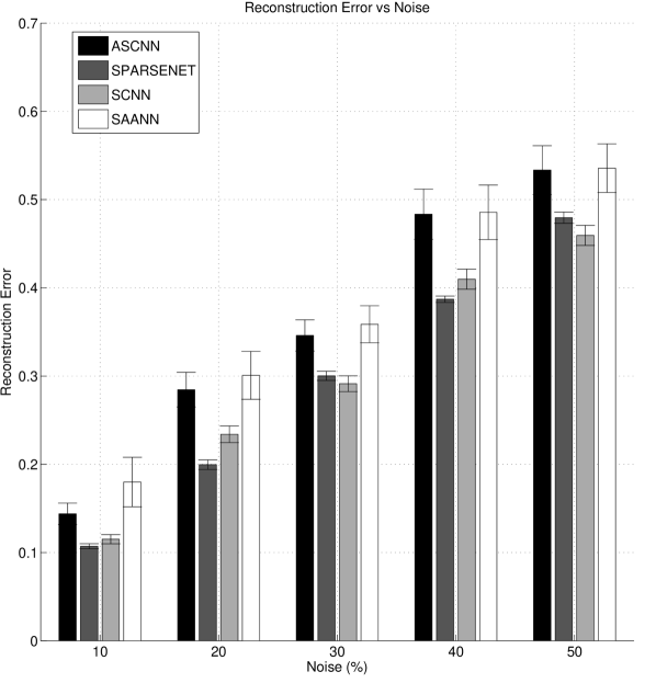
Figure 3: Reconstruction Error versus noise. Noise values correspond to $10\%$, $20\%$, $30\%$, $40\%$ and $50\%$ of missing pixels.

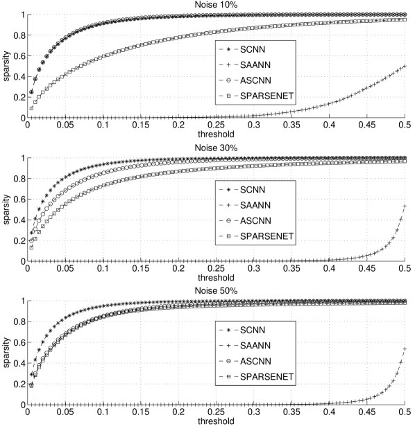
Figure 4: Plot of the sparsity achieved on a test image versus the threshold $Th_{S}$ for different noise values. The best performance is obtained by SCNN which turns out to be the more stable method with respect to increasing percentages of noise.

4.3 Hand-Written Digit Classification

In this test we considered a hand-written digit classification problem. The MNIST dataset [20] is used here. We extracted three datasets: a training set $Digit_{tr}$, a validation set $Digit_{val}$ and a test set $Digit_{T}$. Each image belonging to these datasets was transformed by re-mapping the pixel range value into the interval $[-1,1]$. Each network was applied on the training set using different values of $\lambda$. For each $\lambda$ value a linear SVM was used as multi-class classifier [21]. The classifier was trained with the sparse image representations corresponding to the training set $Digit_{Tr}$, and then it was fed with the sparse image representations corresponding to the validation set $Digit_{val}$. For each network the best solution was chosen on the validation set considering the classification accuracy (defined as the ratio between correctly classified images and the total number of images belonging to the set). Finally, the performances of the networks were computed on the test set $Digit_{T}$ considering the performance of the multi-class classifier when it is fed with the sparse image representations obtained by the previously selected projection dictionaries. The test was organized into two phases. In the first phase, we compared our approach with ASCNN, SAANN and Sparsenet on a reduced subset of the MNIST dataset (see Section 4.3.1). In a second phase, we measured the performance of our approach on the whole MNIST dataset, in order to make a comparison possible with other methods presented in the literature (see Section 4.3.2).

4.3.1 Comparing SCNN with ASCNN, SAANN and Sparsenet

Here SCNN is compared with ASCNN, SAANN and Sparsenet. The test is organized in three parts. In the first part, for a fixed size of the input, we computed classification accuracies on the basis of the data representations of the four networks at varying the number of hidden nodes, i.e., the number of atoms of the reconstruction dictionary. Thus, we evaluated how the inner complexity of each neural network is reflected on its performances. Moreover, we measured the computational times of each network during both learning and validation phase to compare the computational costs of our approach with the other methods. In the second part of the experiment, for each approach we chose the neural architecture with a number of hidden nodes producing a “satisfactory” classification accuracy, and evaluated whether the ability to obtain data representations with high sparsity values was preserved in this case. In particular, in order to get a better insight in the relation between accuracies and sparsity values, we computed first the area under the curve obtained by plotting the sparsity values versus the threshold $Th_{S}$, called sparsity area, and then we computed the accuracies versus sparsity areas. In the last part of the experiment, we evaluated to what extent each approach suffers from the “curse of dimensionality” [22]. Accordingly, fixed the number of hidden nodes we computed the classification accuracies of the four networks at varying sizes of the input.

The sizes of the three datsets $Digit_{tr}$, $Digit_{val}$ and $Digit_{T}$ were chosen equal to $500$ digits. We chose $40$ equispaced values of $\lambda$ in the range $[0.01,20]$ for Sparsenet, and in the range $[0.01,1]$ for the other networks. The dictionary dimension in the first part of the test, Figure 5, was varied from $25$ to $150$ with a step of $25$, and the digits were reshaped into a matrix of dimensions $14\times 14$. Notably, both Sparsenet and SCNN reach high values of classification accuracies using a reduced number of atoms, and the classification accuracy seems to be weakly dependent on this number, whereas ASCNN and SAANN need more than $100$ hidden nodes to reach performances that are comparable to those of Sparsenet and SCNN. In Figure 6 and 7 we show the means and the standard deviations of the computational times at varying the $\lambda$ parameter for each dictionary dimension, and for all methods, during the learning phase and the validation phase, respectively. In Figure 6 one can note that SCNN is uniformly faster than the other methods during the learning phase on all dictionary dimensions. In Figure 7 Sparsenet computational times are not shown because they are an order of magnitude greater than those of the other methods. Also in this case, one can note that SCNN is faster than the other approaches for each dictionary dimension.

In the second part of the test, we fixed the size of the dictionary to $100$ and computed classification accuracies and sparsity areas using $100$ equispaced values of the sparsity parameter $\lambda$. In Figure 8 classification accuracies versus sparsity areas are showed for each network. Figure 8 shows that the best accuracy values are obtained by SCNN and Sparsenet. In particular, Sparsenet reaches the maximum value (0.88) among the selected approaches. By means of SCNN one obtains high accuracy values (more than 0.80) preserving high sparsity values in terms of sparsity area. The other algorithms (ASCNN and SAANN) exhibit high sparsity values but in connection with lower values of classification accuracy only. More specifically, for high sparsity values both SAANN and ASCNN reach accuracy values lower than 0.8. On the whole, SCNN enables one to reach both high accuracy values and high sparsity values.

In the last part of the test, Figure 9, we fixed both the size of the dictionary ($100$) and the size of the training set, while digits were reshaped into a matrix of dimensions from $14\times 14$ to $28\times 28$. From Figure 9, one notices that the accuracy values reached by SCNN and Sparsenet do not seem to be affected by input size. By contrast, ASCNN and SAANN turn out to be strongly dependent on input size.

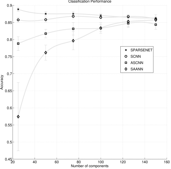
Figure 5: Classification accuracy versus number of components. SCNN achieves high accuracy even with $20$ hidden nodes while ASCNN and SAANN achieve the same performances as SCNN only when more than $100$ hidden nodes are allowed.

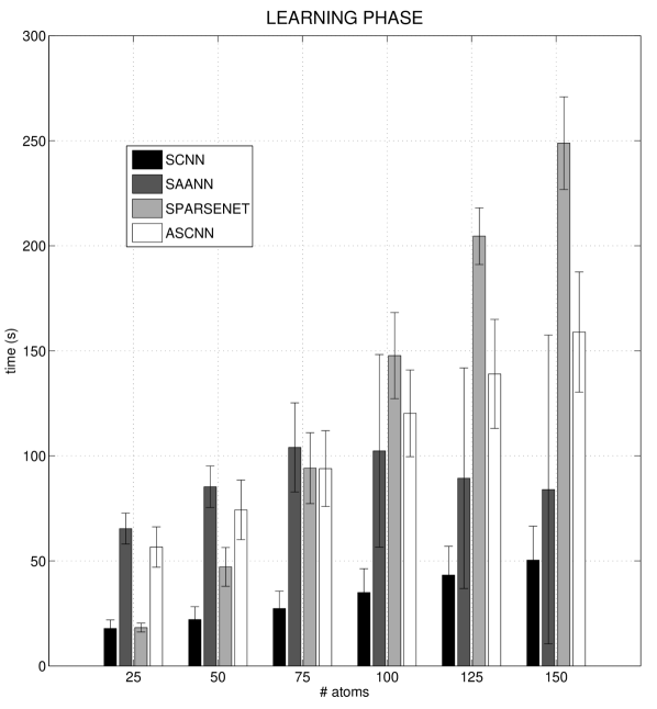
Figure 6: Computational times during the learning phase for each neural network with respect to the dictionary dimension. The bars show the means of the computational times at varying the $\lambda$ parameter. The error bars represent the standard deviations.

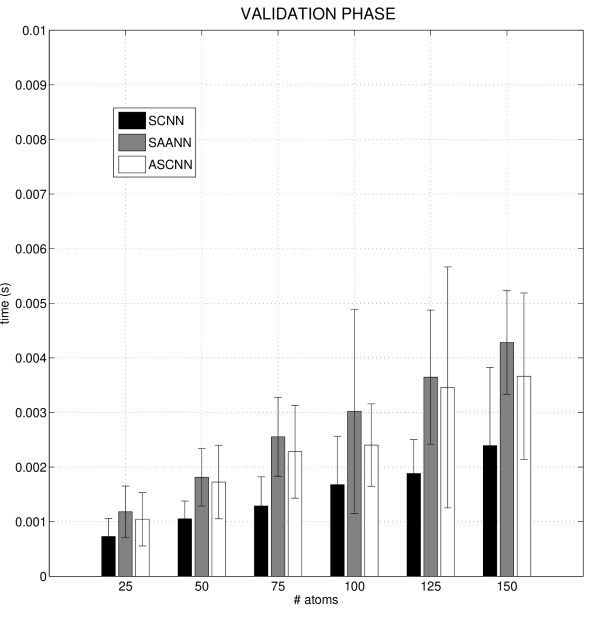
Figure 7: Computational times during the validation phase for each neural network with respect to the dictionary dimension. Sparsenet computational times are not shown because they are an order of magnitude greater than those of the other neural networks. The bars show the means of the computational times at varying the $\lambda$ parameter. The error bars represent the standard deviations.

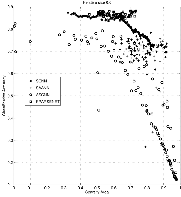
Figure 8: Classification accuracy values versus sparsity areas. SCNN seems to achieve the best compromise between sparsity area and accuracy in correspondence to sparsity area $\sim 0.8$ and accuracy $\sim 0.8$.

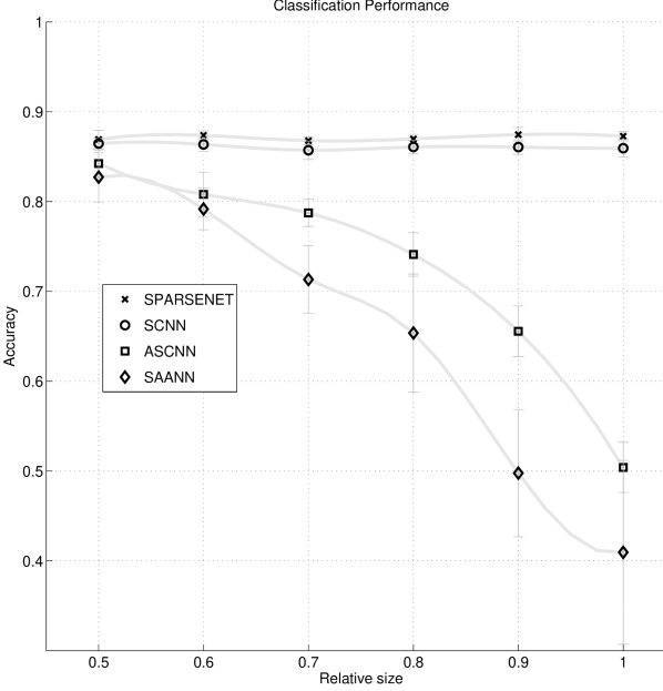
Figure 9: Classification accuracy versus relative size. Leaving fixed the number of hidden nodes and the size of the training set while increasing the number of inputs by reshaping the digits, SCNN is very robust with respect to the “course of dimensionality”.

4.3.2 SCNN Error Rate and Noise tolerance

In this phase the sizes of three datasets $Digit_{tr}$, $Digit_{val}$ and $Digit_{T}$ were of $50000$, $10000$ and $10000$ digits, respectively. The test was organized in two parts. In the first part, we measured the error rate of the linear multi-class classifier on the sparse digit representations obtained by our approach at varying numbers of hidden nodes. The experimental setting was basically left unchanged with respect to the previously described setting. In particular, we used $10$ equispaced values of $\lambda$ in the range $[0.02,0.2]$, and a number of hidden node equal to $400,800,1200$ and $1600$. The sparse representations of $Digit_{tr}$, $Digit_{val}$ and $Digit_{T}$ were obtained by applying the projection dictionary followed by a soft-thresholding operation.

In the second part of the test, we evaluated the effect of noise on the performance of SCNN. In particular we compared SCNN, raw-data and SCNN with a re-learning phase on the test set (without using a projection dictionary) . We obtained $5$ versions of the MNIST dataset by adding Gaussian white noise of mean $0$ and standard deviation $\sigma=0.02,0.04,0.06,0.08$. On each dataset we repeated the previously described experimental setting with a number of hidden nodes equal to $400$.

The results show that our approach leads to performances that are quite good for this non-linear classification task, insofar as they are consistently better than those obtained by means of linear classifiers on raw images across various projection dictionary sizes. In addition, the best error rate was equal to $2.0\%$ which is better than or comparable to state-of-the-art results that are based on unsupervised feature learning plus linear classification without using additional image geometric information (see Table 1 and 2). In particular, we note that the error rate of deep belief network is very similar to that obtained by SCNN. Moreover, our approach seems to be little affected by noise (see Table 3).

Methods	Error rate (%)
Raw image $+$ Linear SVM	12 [23]
Sparse coding $+$ linear SVM	2.02 [24]
Deep Belief Network $+$ linear SVM	1.90 [23]
Stacked RBM network	1.2 [25]
Map transformation cascade $+$ linear SVM	1.90 [24]
Local Kernel smoothing	3.48 [23]
VQ coding $+$ linear SVM	3.98 [23]
Laplacian eigenmap $+$ linear SVM	2.73 [23]
Large Conv. Net, unsup. pretraining	0.53 [26]
Local coordinate coding $+$ linear SVM	1.90 [23]
Human	0.2 [27]

Table 1: Error rates (%) of MNIST classification with different methods.

# hidden units	400	800	1200	1600
SCNN $+$ linear SVM	2.7	2.4	2.1	2.0

Table 2: Error rates (%) of MNIST classification by SCNN $+$ linear SVM against different number of hidden units.

Noise ($\sigma$)	0.02	0.04	0.06	0.08
Raw image $+$ linear SVM	6.3	6.8	7.7	8.7
SCNN $+$ linear SVM	3.8	4.2	4.7	5.5
SCNN with re-learning $+$ linear SVM	4.9	4.8	5.7	6.9

Table 3: Error rates (%) of MNIST classification by SCNN $+$ linear SVM with a number of hidden units equal to $400$ against different noise values. These value are also compared with those obtained by raw images and SCNN with a re-learning phase on the test set (without using a projection dictionary).

5 Conclusions

In this paper we showed that a linear two-layer neural netwok (SCNN) can be profitably used to achieve sparse data representations for solving machine learning problems.

In our approach hidden layer linearity and the specific choice of error function allow one to explicitly define learning rate values which ensure linear rates of convergence in the minimization of error function and convergence of both reconstruction (decoder) and projection (encoder) dictionaries towards a minimizer [18, 28, see]. Moreover, we have to set the number of units of just one hidden layer, unlike deep network approaches, and the linearity of the hidden layer allows one to perform a learning process which is computationally less expensive than a non-linear approach for a time constant. In this sense, we claim that our architecture is a comparatively " simple" one.

SCNN reaches a very similar reconstruction error compared to PCA as described in Section 4.1. Interestingly, by means of our approach, we obtained performances that are comparable to or better than non-linear methods. More specifically, the experiments in Section 4.2 and 4.3.1 show that our approach produces sparse data representations enabling one to solve standard machine learning problems. SCNN outperforms ASCNN and SAANN in all cases; and its performances are comparable to those of Sparsenet, which does not use an encoder to project unseen data to sparse code, but requires iteration of a learning process. In the hand-written digit classification problem (see Section 4.3.2), our results are competitive with respect to state-of-the-art results that are based on unsupervised feature learning plus linear classification without using additional image geometric information. In addition, our approach seems to be little affected by noise.

It is worth noting, in connection with Section 4.2, that during the test phase our approach (SCNN) reaches high sparsity values comparable with or better than the values obtained by ASCNN and Sparsenet that make use of non linear activation functions and a new learning process, respectively. SAANN has sparsity values that are much lower than those obtained by all other methods. Figure 4 shows that the SCNN linear encoder projects input data with a degree of sparsity greater than or equal to that obtained by ASCNN and Sparsenet for different noise levels. In connection with Section 4.3.1, it is worth noting that both SCNN and Sparsenet achieve high accuracy values (more than 0.80) preserving high sparsity values in terms of sparsity area. ASCNN and SAANN exhibit also high sparsity values but in correspondence of lower values of classification accuracy. In the hand-written digit classification problem (see Section 4.3.2, linear projection dictionary followed by soft-thresholding operator enable one to obtain an error rate equal to about $2\%$, that is, a better value than that obtained by other approaches such as Local Kernel smoothing, VQ coding and Laplacian eigenmap. Furthermore, this value is comparable to standard sparse coding approaches and deep network (see Table 1 and 2).

It is worth noting that the learning process based on an alternate updating of the dictionaries $\mathbf{C}$ and $\mathbf{D}$ (see ASCNN and SCNN learning processes, sections 2 and 3) appears to lead to better results than the update involving two dictionaries simultaneously (see SAANN learning process, Section 2). In fact, SAANN achieves in many cases worse results than SCNN and ASCNN (see for example figures 2, 3, and 6).

Altogether, these results suggest that linear encoders can be used to obtain sparse data representations that are useful in the context of machine learning problems, providing that an appropriate error function is used during the learning phase. In particular, on the basis of some suggestions made in [29, 2] we introduced a term in the error function which enables one to obtain a sparse code which is as similar as possible to the output of the encoder.

References

- [1] M Aharon, M Elad, and A Bruckstein. K-svd: An algorithm for designing overcomplete dictionaries for sparse representation. IEEE Transactions on Signal Processing, 54(11):4311–4322, 2006.
- [2] M Ranzato, Y-lan Boureau, and Yann LeCun. Sparse feature learning for deep belief networks. In Advances in neural information processing systems, pages 1185–1192, 2007.
- [3] Julien Mairal, Francis Bach, Jean Ponce, and Guillermo Sapiro. Online learning for matrix factorization and sparse coding. J. Mach. Learn. Res., 11:19–60, March 2010.
- [4] R. Jenatton, J. Mairal, G. Obozinski, and F. Bach. Proximal methods for hierarchical sparse coding. Arxiv preprint arXiv:1009.2139, 2010.
- [5] C Basso, M Santoro, A Verri, and S Villa. Paddle: Proximal algorithm for dual dictionaries learning. CoRR, abs/1011.3728, 2010.
- [6] Geoffrey E Hinton, Simon Osindero, and Yee-Whye Teh. A fast learning algorithm for deep belief nets. Neural computation, 18(7):1527–1554, 2006.
- [7] Yoshua Bengio. Learning deep architectures for ai. Foundations and trends® in Machine Learning, 2(1):1–127, 2009.
- [8] Adam Coates, Andrew Y. Ng, and Honglak Lee. An analysis of single-layer networks in unsupervised feature learning. Journal of Machine Learning Research - Proceedings Track, 15:215–223, 2011.
- [9] Yann Dauphin and Yoshua Bengio. Big neural networks waste capacity. CoRR, abs/1301.3583, 2013.
- [10] X. Zeng, S. Luo, and Q. Li. An associative sparse coding neural network and applications. Neurocomputing, 73(4-6):684–689, 2010.
- [11] G.S.V.S. Sivaram, S. Ganapathy, and H. Hermansky. Sparse auto-associative neural networks: Theory and application to speech recognition. In Eleventh Annual Conference of the International Speech Communication Association, pages 2270–2273, 2010.
- [12] G. E. Hinton and R. R. Salakhutdinov. Reducing the dimensionality of data with neural networks. Science, 313(5786):504–507, 2006.
- [13] M. Ranzato, Fu Jie Huang, Y.-L. Boureau, and Y. LeCun. Unsupervised learning of invariant feature hierarchies with applications to object recognition. In Computer Vision and Pattern Recognition, 2007. CVPR ’07. IEEE Conference on, pages 1–8, 2007.
- [14] K. Kavukcuoglu, M. Ranzato, and Y LeCun. Fast inference in sparse coding algorithms with applications to object recognition. CoRR, abs/1010.3467, 2010.
- [15] Yongkang Wong, Mehrtash Tafazzoli Harandi, and Conrad Sanderson. On robust face recognition via sparse encoding: the good, the bad, and the ugly. CoRR, abs/1303.1624, 2013.
- [16] B.A. Olshausen et al. Emergence of simple-cell receptive field properties by learning a sparse code for natural images. Nature, 381(6583):607–609, 1996.
- [17] Martin Rehn and Friedrich T Sommer. A network that uses few active neurones to code visual input predicts the diverse shapes of cortical receptive fields. Journal of computational neuroscience, 22(2):135–146, 2007.
- [18] A. Beck and M. Teboulle. Fast gradient-based algorithms for constrained total variation image denoising and deblurring problems. Image Processing, IEEE Transactions on, 18(11):2419–2434, 2009.
- [19] D. Martin, C. Fowlkes, D. Tal, and J. Malik. A database of human segmented natural images and its application to evaluating segmentation algorithms and measuring ecological statistics. In Proc. 8th Int’l Conf. Computer Vision, volume 2, pages 416–423, July 2001.
- [20] Yann LeCun, Léon Bottou, Yoshua Bengio, and Patrick Haffner. Gradient-based learning applied to document recognition. Proceedings of the IEEE, 86(11):2278–2324, 1998.
- [21] T Hastie, R Tibshirani, and JH Friedman. The Elements of Statistical Learning: Data Mining, Inference, and Prediction. Springer, corrected edition, 2003.
- [22] Christopher M Bishop. Neural networks for pattern recognition. Oxford university press, 1995.
- [23] Kai Yu, Tong Zhang, and Yihong Gong. Nonlinear learning using local coordinate coding. In NIPS, volume 9, page 1, 2009.
- [24] Ângelo Cardoso and Andreas Wichert. Handwritten digit recognition using biologically inspired features. Neurocomputing, 99:575–580, 2013.
- [25] Hugo Larochelle, Yoshua Bengio, Jérôme Louradour, and Pascal Lamblin. Exploring strategies for training deep neural networks. The Journal of Machine Learning Research, 10:1–40, 2009.
- [26] Kevin Jarrett, Koray Kavukcuoglu, M Ranzato, and Yann LeCun. What is the best multi-stage architecture for object recognition? In Computer Vision, 2009 IEEE 12th International Conference on, pages 2146–2153. IEEE, 2009.
- [27] Yann LeCun, LD Jackel, Léon Bottou, Corinna Cortes, John S Denker, Harris Drucker, Isabelle Guyon, UA Muller, E Sackinger, Patrice Simard, et al. Learning algorithms for classification: A comparison on handwritten digit recognition. Neural networks: the statistical mechanics perspective, 261:276, 1995.
- [28] P.L. Combettes, V.R. Wajs, et al. Signal recovery by proximal forward-backward splitting. Multiscale Modeling and Simulation, 4(4):1168–1200, 2006.
- [29] Curzio Basso, Matteo Santoro, Alessandro Verri, and Silvia Villa. Paddle: proximal algorithm for dual dictionaries learning. In Artificial Neural Networks and Machine Learning–ICANN 2011, pages 379–386. Springer, 2011.