Interplay between pulsations and mass loss in the blue supergiant 55 Cygnus = HD 198 478

Abstract

Context. Blue supergiant stars are known to display photometric and spectroscopic variability that is suggested to be linked to stellar pulsations. Pulsational activity in massive stars strongly depends on the star’s evolutionary stage and is assumed to be connected with mass-loss episodes, the appearance of macroturbulent line broadening, and the formation of clumps in the wind.

Aims. To investigate a possible interplay between pulsations and mass-loss, we carried out an observational campaign of the supergiant 55 Cyg over a period of five years to search for photospheric activity and cyclic mass-loss variability in the stellar wind.

Methods. We modeled the H, He i, Si ii, and Si iii lines using the nonlocal thermal equilibrium atmosphere code FASTWIND and derived the photospheric and wind parameters. In addition, we searched for variability in the intensity and radial velocity of photospheric lines and performed a moment analysis of the line profiles to derive frequencies and amplitudes of the variations.

Results. The H$\alpha$ line varies with time in both intensity and shape, displaying various types of profiles: P Cygni, pure emission, almost complete absence, and double or multiple peaked. The star undergoes episodes of variable mass-loss rates that change by a factor of 1.7–2 on different timescales. We also observe changes in the ionization rate of Si ii and determine a multiperiodic oscillation in the He i absorption lines, with periods ranging from a few hours to 22.5 days.

Conclusions. We interpret the photospheric line variations in terms of oscillations in p-, g-, and strange modes. We suggest that these pulsations can lead to phases of enhanced mass loss. Furthermore, they can mislead the determination of the stellar rotation. We classify the star as a post-red supergiant, belonging to the group of $\alpha$ Cyg variables.

1 Introduction

Blue supergiants (BSGs) are evolved, luminous objects that often display strong photometric and spectroscopic variability (e.g., Rosendhal 1973; Kaufer et al. 1997; Waelkens et al. 1998; Mathias et al. 2001; Kaufer et al. 2006; Lefever et al. 2007; Clark et al. 2010). Long-term space-based photometry has linked this variability to stellar pulsations, establishing a new instability domain in the Hertzsprung-Russell (HR) diagram region populated by BSGs (Saio et al. 2006). The presence of pulsations in BSGs requires that excited modes are reflected either at an intermediate convection zone connected to the hydrogen-burning shell (Saio et al. 2006; Godart et al. 2009), or at the top of the chemical composition gradient region surrounding the radiative He core (Daszyńska-Daszkiewicz et al. 2013).

While BSGs in the vicinity of the main sequence are found to pulsate in both pressure (p-modes with periods of hours to about one day) and gravity modes (g-modes with periods of 2-10 days), objects slightly more evolved to the red are predicted to pulsate in pure g-modes (Saio et al. 2006). However, Kraus et al. (2012) recently discovered a periodic variability of 1.6 hours in the late-type BSG star HD 202 850. Existing pulsation models do not predict such short periods; this emphasizes the current deficiency in our knowledge of the pulsation activity in BSGs.

As massive stars can cross the BSG domain more than once, the pulsational activity of these stars can drastically change between their red- and blueward evolution (Saio et al. 2013). When compared with their less-evolved counterparts, BSGs on a blue loop, or blueward evolution, tend to undergo significantly more pulsations, even including radial strange-mode pulsations (with periods of 10-100 or more days), as observed in $\alpha$ Cygni variables.

Additionally, the photospheric line profiles of BSGs typically contain some significant extra broadening, so-called macroturbulence (Abt 1958; Conti & Ebbets 1977), which is often on the same order as rotational broadening (Ryans et al. 2002; Simón-Díaz & Herrero 2007; Markova & Puls 2008). Recent evidence links macroturbulence and line profile variability to stellar pulsational activity (Aerts et al. 2009; Simón-Díaz et al. 2010a, b), providing additional proof for the presence of pulsations in BSGs.

BSGs lose mass via their line-driven winds, but the rates at which the material is lost are still highly debated. Diverse spectral ranges trace distinct wind regions, and comparison of mass-loss rates obtained from various methods typically results in values that can differ by a factor 2–10. In addition, the observed complex wind structures seen in the H$\alpha$ variability of BSGs (e.g., Kaufer et al. 1996; Markova et al. 2008), for instance, imply that these objects cannot have smooth spherically symmetric winds. Spectropolarimetric observations revealed no evidence of magnetic fields (Shultz et al. 2014). Instead, the winds of BSGs are found to be clumped (Prinja & Massa 2010). Micro- and macro-clumping severely influence both mass-loss determination and line profile shapes of not only resonance lines, but also H$\alpha$ (e.g., Sundqvist et al. 2010, 2011, 2014; Šurlan et al. 2012, 2013). The onset of clumping in the winds of massive stars could be due to line-driven instability (see, e.g., Feldmeier 1998). Perturbations leading to this instability might be initiated by pulsational activity, at least in the vicinity of the stellar photosphere. Moreover, strange mode pulsations have been suggested to cause time-variable mass loss in luminous, evolved massive stars (see Glatzel et al. 1999; Aerts et al. 2009; Puls et al. 2011). The first observational evidence of these modes was found in the massive BSG HD 50 064 (Aerts et al. 2010b).

The ability of BSGs to maintain stable pulsations opens a completely new perspective in studying these stars. Based on established methods from asteroseismology, it will be possible to investigate not only the stellar atmospheres from which the mass-loss and possible onset of wind clumping are initiated, but also the deep interior of the stars, revealing important physical properties, such as internal structure, rotation, and mixing. Knowledge of these parameters is of vital importance for our understanding of the post-main sequence evolution of massive stars, as these are key input parameters to modern stellar evolution calculations. This emphasizes the need for further investigations, both theoretically and observationally, to improve our understanding of pulsational activity in BSGs in different evolutionary stages.

To investigate, in particular, the possible interplay between pulsations and mass-loss, we initiated an observational campaign to search for pulsational activity and cyclic mass-loss variability in stellar winds for a sample of bright BSGs. Here we report on our results for the object 55 Cyg.

2 The star

55 Cyg (HD 198 478, MWC 353, HR 7977, HIP 102 724, $\alpha$ = $20^{\mathrm{h}}\,48^{\mathrm{m}}\,56\,\aas@@fstack{s}291$ and $\delta$ = $\,+46^{\degr}\,06^{\arcmin}$ $50\,\aas@@fstack{\prime\prime}88$; 2000) is a bright star located in the Cyg OB7 association (Humphreys 1978) that was classified as B3 Ia by Morgan & Roman (1950). Its hipparcos parallax of $1.40\pm 0.17$ mas (van Leeuwen 2007) places the star at a distance of $714\pm 86$ pc. The interstellar visual extinction toward 55 Cyg was found to be 1.62 mag (Barlow & Cohen 1977; Humphreys 1978).

Studies of its photospheric lines revealed two important facts: different elements typically display different radial velocities (e.g., Hutchings 1970), while the same lines show strong variations with time. For instance, Underhill (1960) described radial velocity variations of 25 km s^-1, with no evidence that the changes found were periodic. Later, Granes (1975) collected 34 spectra, distributed over 15 consecutive nights, and found that the radial velocity curves oscillate with a period of 4-5 days, in addition to photospheric motions on timescales about three times longer.

Photometric observations are found to display microvariability, but clear periodicities are difficult to establish. While Rufener & Bartholdi (1982) reported an 18-day variability in their V-band magnitudes, Koen & Eyer (2002) found a periodicity of 4.88 days using hipparcos data. On the other hand, no indication for clear periodicities were seen by Percy & Welch (1983), van Genderen (1989), and Lefèvre et al. (2009).

The H$\alpha$ line in 55 Cyg is also highly variable. While Underhill (1960) and Rzaev (2012) remarked that in their spectra the H$\alpha$ line maintained a P Cygni profile, but with highly variable strength, Ebbets (1982) noted that during one of his observations, H$\alpha$ showed additional faint emission wings, which were not visible anymore in the spectrum he took two months later. Furthermore, Maharramov (2013) discovered that H$\alpha$ can even completely disappear from the spectrum.

The stellar rotation velocity, projected on the line of sight ($v\sin i$), and the terminal wind velocity ($v_{\infty}$) are also highly variable or uncertain. For both, broad ranges are found in the literature. Values for $v\sin\,i$ range from 0 km s^-1 (Slettebak & Howard 1955) to a maximum of 61 km s^-1 (Howarth et al. 1997). The latter was obtained from lines in the IUE spectra. Other determinations based on optical spectral lines and different techniques include 42 km s^-1 (Day & Warner 1975), $49\pm 1$ km s^-1 (Gies & Lambert 1992), $45\pm 20$ km s^-1 (McErlean et al. 1999), $35\pm 9$ km s^-1 (Abt et al. 2002), and 39 km s^-1 (Markova & Puls 2008). The terminal wind velocity is much harder to determine. Based on different lines in the IUE spectra, Prinja et al. (1990) obtained 470 km s^-1 from the C iv line, while Prinja & Massa (2010) derived a higher value of 560 km s^-1 from Si iv. Both values are lower than predictions from line-driven wind theory, however, which delivers a value of $\sim 690$ km s^-1 (see, e.g., Krtička & Kubát 2001). Conversely, Markova & Puls (2008) noted that the observed value of 470 km s^-1 is too high to give satisfactory fits to their H$\alpha$ line, which would agree much better with a terminal wind velocity of only $\sim 200$ km s^-1. These authors speculated that 55 Cyg might have a time-variable wind velocity.

There is also scatter in the derived stellar parameters. Although the determination of fundamental parameters could be biased by the technique used, different values of $T_{\rm{eff}}$ are found using models built on similar approaches. $T_{\rm eff}$ measurements based on the Balmer discontinuity give values of 16 450 K (the color index method of Gies & Lambert 1992) and $15\,380\pm 860$ K (the BCD spectrophotometric method of Zorec et al. 2009), respectively. Using nonlocal thermal equilibrium (non-LTE) plane-parallel hydrostatic stellar atmosphere and the Si ionization balance, the derived $T_{\rm{eff}}$ values are 18 000 K (McErlean et al. 1999), 18 500 K (Monteverde et al. 2000), and 17 000 K (Jurkić et al. 2011), while non-LTE line- and wind-blanketed model atmospheres provide values of 16 500 K (Crowther et al. 2006) and 17 500 K (Searle et al. 2008; Markova & Puls 2008). In all cases, the surface gravity determinations are around $\log\,g=2.2\pm 0.1$ (cf. Jurkić et al. 2011).

As H$\alpha$ is a fundamental mass-loss diagnostic (e.g., Puls et al. 1996), it can be expected that model fits to observations obtained at different periods (with correspondingly varied shape and line strength) result in different mass-loss rates. And the values clearly vary by a substantial amount. While Searle et al. (2008) found $\dot{M}=5\times 10^{-7}$ M_⊙yr^-1, the value of Crowther et al. (2006) is a factor of two lower, even though both works used the same terminal wind velocity value of 470 km s^-1. In addition, Markova & Puls (2008) obtained a rather large uncertainty in their mass-loss values $(1.175-4.07)\times 10^{-7}$ M_⊙yr^-1, which is due to the high uncertainty in the wind terminal velocity (200 km s^-1 vs 470 km s^-1). All of these investigations used smooth (i.e., unclumped) winds.

Concerning the possible evolutionary stage of 55 Cyg, Underhill (1969) mentioned that the observed H$\gamma$ line profile was too shallow, which could indicate that 55 Cyg is H-poor, and hence a post-red supergiant. A similar conclusion was drawn by Lennon et al. (1993), Gies & Lambert (1992), Crowther et al. (2006), and Searle et al. (2008) based on the CNO-processed material seen in its optical spectra, in particular, its strong N-enrichement. Markova & Puls (2008) additionally concluded that the star probably is enriched in He. These authors also found a rather low spectroscopic mass of $\sim 11$ M_⊙ compared to the star’s high luminosity, which places it on an evolutionary track of an initial mass of 25 M_⊙. Additional support for its evolved nature comes from van Genderen (1989), who listed 55 Cyg as an $\alpha$ Cygni variable (i.e., a luminous, photometrically variable supergiant of spectral type B and A). If this classification is correct, then 55 Cyg should display numerous pulsation modes, including radial strange modes (Saio et al. 2013).

3 Observations

We spectroscopically monitored 55 Cyg between 2009 August 15 and 2013 October 22. We obtained a total of 344 spectra, distributed over 64 nights, with the Coudé spectrograph attached to the Perek 2 m telescope at Ondřejov Observatory (Šlechta & Škoda 2002). Until the end of May 2013, the observations were taken with the 830.77 lines mm^-1 grating and a SITe $2030\times 800$ CCD. Beginning in June 2013, we used the newly installed PyLoN $2048\times 512$BX CCD. With both detectors, a spectral resolution of $R\simeq 13\,000$ in the H$\alpha$ region was achieved, and the wavelength coverages were from 6253 Å to 6764 Å for the old CCD and from 6263 Å to 6744 Å with the new one. For wavelength calibration, a comparison spectrum of a Th-Ar lamp was taken immediately after each exposure. The stability of the wavelength scale was verified by measuring the wavelength centroids of O i sky lines. The velocity scale remains stable within 1 km s^-1. Individual exposure times range from 400 s to 2700 s, and, for all spectra, the achieved signal-to-noise (S/N) ratio was higher than 300. During the nights of 2013 July 19–22 and 2013 August 10–12, we achieved S/N values of more than 500, allowing for high-quality time series, covering several hours of continuous observation.

We also obtained a series of echelle spectra using the Poznan Spectroscopic Telescope at the Winer Observatory in Arizona, USA. Observations were carried out from 2013 October 17 to 2013 November 7, and a total of 41 spectra were acquired, covering the wavelength range 3900 to 8677 Å,  with a spectral resolution of $R=40\,000$. Each spectrum has an exposure time of 1800 s and a S/N of $\sim 120-180$.

All data were reduced and the heliocentric velocity corrected using standard IRAF tasks. We also observed a rapidly rotating star (HR 7880, Regulus, $\zeta$ Aql) once per night to perform the telluric correction.

Figure 1: Spectrum of 55 Cyg taken in the H$\alpha$ region with the Perek 2m telescope at Ondřejov Observatory.

Figure 2: Night-to-night variation in the H$\alpha$ line in the observing period 2013 July 19 to August 12. This period shows all of the typical profile shapes: P Cygni, pure emission, almost complete absence, and double and multiple peaked.

A typical Ondřejov spectrum is shown in Fig. 1. In general, the overall appearance of the full optical spectrum is very similar to the ones presented by Lennon et al. (1992) and Chentsov & Sarkisyan (2007). Interesting is the shallow, but broad emission component centered on the H$\alpha$ line, which is noticeable in each of our spectra, while it was reported only once in the literature (Ebbets 1982). The extent of the emission wings measured from our spectra is $\pm 1200$ km s^-1. Such broad emission components typically originate from incoherent electron scattering (see, e.g., McCarthy et al. 1997; Kudritzki et al. 1999).

The H$\alpha$ line displays time variations in both intensity and shape, showing various types of profiles: P Cygni, pure emission, almost complete absence, and double or multiple peaked. As an example, see Fig. 2. Similar variability of the H$\alpha$ line has been observed in other BSGs that belong to the group of $\alpha$ Cygni variables (e.g., Kaufer et al. 1996).

4 Results

4.1 Line profile modeling

To quantify and analyze the spectral line variation of 55 Cyg, we simultaneously fit observed line profiles of several representative transitions of H, He and Si atoms with synthetic line models computed with the code Fast Analysis of STellar atmospheres with WINDs (FASTWIND). This is a non-LTE, spherically symmetric model atmosphere code that enables computating continuum and line radiation fluxes and provides a set of parameters that describe the photospheric and wind structure (Santolaya-Rey et al. 1997; Puls et al. 2005). The code includes line blocking and blanketing effects and consistently calculates the temperature structure (see details in Kubát et al. 1999). The wind velocity distribution is computed using the so-called $\beta$-law.

For the fundamental stellar parameters ($T_{\rm eff},\log\,g$) we mainly used the Arizona spectra. They cover the H$\gamma$ and H$\delta$ lines (known as excellent surface gravity sensors) and the He i $\lambda$ 4471 triplet line (considered a good gravity indicator, with some sensitivity to $T_{\rm eff}$ as well, Lefever et al. 2007). In addition, we modeled the singlet transitions of He i $\lambda$ 6678 Å and He i $\lambda$ 4713 Å, and the lines of Si ii $\lambda\lambda$ 4128, 4130 Å, and Si iii $\lambda$ 4552 Å. These Si lines are also excellent temperature indicators (Markova & Puls 2008). Unfortunately, the Ondřejov spectra cover a more restricted wavelength interval, providing only the He i $\lambda$ 6678 Å line. Although the Ondřejov spectra have a lower resolution, they have significantly higher S/N ratios than the Arizona spectra.

Another input model parameter is the stellar radius. This value should be derived in an independent way, such as the de-reddened absolute magnitude or the spectral energy distribution. Different authors used these methods to derived the radius of 55 Cyg and obtained values ranging from $38\,R_{\sun}$ (Markova & Puls 2008) to $83\,R_{\sun}$ (Gies & Lambert 1992). Because of the large discrepancy in the literature values, we employed other methods. Using the BCD parameters, based on a reddening-independent method (Zorec et al. 2009), we obtain a bolometric magnitude of $-8.5\pm 0.3$ mag, which leads to $\log\,L/L_{\sun}=5.3\pm 0.1$ and $R=61\pm 8\,R_{\sun}$. This bolometric magnitude agrees with the determination reported by Barlow & Cohen (1977), who estimated $M_{\rm V}=-6.8$ mag from the 10 $\mu$m excess emission. With the bolometric correction of 1.7 (Flower 1996), we derive $M_{\rm{bol}}=-8.6$ mag, in agreement with the BCD method. The radius obtained from these two methods also agrees with the value of 61 R_⊙, derived by Pasinetti Fracassini et al. (2001) based on measurements of the stellar angular diameter from infrared photometry by Blackwell & Shallis (1977).

The wind parameters were derived by modeling the H$\alpha$ line. To compute the synthetic line profiles for 55 Cyg, we started from a set of initial values for both photospheric and wind parameters, taken from the literature (see Sect. 2). However, these values did not deliver good fits, so that we extended the range of parameters, looking for the best fit in a “by-eye” procedure. For this, we treated all model parameters ($T_{\rm{eff}}$, $\log\,g$, $\beta$, $\dot{M}$, $v_{\infty}$, $v_{\rm{macro}}$, and $v_{\rm{rot}}$) as free values and computed a large grid of synthetic line profiles. The parameters $v_{\rm{micro}}$ and $R_{*}$ were initially fixed at 10 km s^-1 and 61 R_⊙ , respectively, and then were slightly varied to obtain improved fits. We selected the best fit to the observations and verified the consistency of some of the individual parameters, which are not independent variables. For example, the stellar radius and the surface gravity should obey the relation $g\,R_{*}^{2}\approx$ constant. To fit the terminal velocity, we preferentially considered the values that reproduce the blueshifted absorption component of the H$\alpha$ P Cygni profile. Otherwise, for profiles with pure emission, we derived the terminal velocity based mainly on the H$\alpha$ line width.

Using the FASTWIND code, we explored the sensitivity of the model parameters that characterize both the photosphere and the wind. However, we should keep in mind that there are two sources of errors. One results from the modeling, in which the involved uncertainties result from the statisitcal standard deviation and are obtained using the best-fit model. The second refers to the inaccuracy of the input parameters, that is, the radius, resulting from the uncertainties in the stellar distance and hence luminosity. But when the distance is fixed, any deviation in the parameters larger than the statistical error indicates possible variability in the physical parameters.

To determine the statistical uncertainty of the parameters, we used the best-fit model and tested different values of each parameter, one at a time, keeping all other parameters fixed. We have the advantage of the many high-resolution and high S/N ratio spectra obtained in Arizona, taken over a sequence of consecutive days. This enabled us to distinguish errors on the mean values of the studied parameters from real changes of the physical conditions.

From fits to the Si ii and Si iii lines we observe uncertainties of 300 K - 500 K in $T_{\rm eff}$. We also find that the H$\alpha$ emission is sensitive to changes in $T_{\rm eff}$ of $\sim 300$ K. From the H$\gamma$ and H$\delta$ wings, the statistical error in $\log\,g$ is 0.05 dex, but due to large uncertainties in other parameters (e.g., the radius), the error could be slightly larger, but still below 0.1 dex. This latter is what we use in the tables as upper limit. The uncertainties in the rotational, micro- and macroturbulent velocities depend on the modeled line transition. Error bars in $v_{\rm micro}$ are 2 km s^-1 for the He and Si lines, and 5 km s^-1 for the H lines, except for H$\alpha$, for which the error is about 10 km s^-1. We find errors of 5 km s^-1 in $v_{\rm rot}$ and $v_{\rm macro}$ for H$\gamma$, H$\delta$, He, and Si lines, and of 5 km s^-1 and 10 km s^-1 for H$\alpha$. For H$\beta$, our error estimates for $v_{\rm rot}$ and $v_{\rm macro}$ are $\sim 20$ km s^-1. To derive the wind parameters, we considered the shape and intensity of the absorption and emission components of the H$\alpha$ line. We find noticeable line variations with changes in $\dot{M}$ of about $0.1\times 10^{-7}$M_⊙ yr^-1 and 10% in $v_{\infty}$ (although the error in $v_{\infty}$ can reach up to 30% if H$\alpha$ displays a pure absorption line). These adopted uncertainties are overestimations because they are larger than or equal to the standard statistical deviation computed with the model parameters of the Arizona data, which correspond to a term of 21 days showing small or moderate spectral variations. Unfortunately, even if we can check the sensitivity of $\dot{M}$ by varying the parameters of the model, we cannot provide an accurate value of this quantity because this depends on the uncertainty of the stellar distance. To evaluate the error in relation to the accurate value, we performed an error propagation using the optical depth parameter $Q=\dot{M}/(v_{\infty}R_{*})^{1.5}$, which results from the model calculations. To compute $Q,$ we selected the observations of Arizona (listed in Table 1, $\log Q=-12.975\pm 0.066$) because they were taken during many consecutive days and the line profiles did not show huge variations. Assuming the scatter in the bolometric magnitude $\Delta M_{\rm bol}\simeq\pm 0.3$, that is, $\Delta\log L/L_{\odot}\simeq 0.12$, and the error in $T_{\rm eff}\simeq 500$ K, we obtain $\Delta\log R_{*}/R_{\odot}\simeq 0.04$. With our uncertainty of 10% in $v_{\infty}$ and the statistical error $\Delta\log Q\simeq\pm 0.07$, the uncertainty in $\Delta\dot{M}/\dot{M}\simeq 0.3$.

The best-fit values (and corresponding statistical deviations) for the photospheric and wind parameters derived for each observation are given in Tables 1 (Arizona data) and 2 (Ondřejov data). We adopt solar abundances for all elements, but discuss the validity, in particular with respect to the He abundance, in Sect. 4.1.4.

Figure 3 shows a sequence of model fits to simultaneous observations of H$\alpha$, H$\beta$, H$\gamma$, H$\delta$, He i $\lambda$ 6678 Å, He i $\lambda$ 4471 Å,  and He i $\lambda$ 4713 Å  line spectra taken in Arizona during 15 successive nights in 2013 (see also Table 1). The fits to the lines of Si ii $\lambda\lambda$ 4128, 4130 Å, and Si iii $\lambda$ 4552 Å  are shown in Fig. 7. We obtained very good fits for the whole sample of lines, with the exception of the blue wing of He i $\lambda$ 4471 Å, where we observe a tiny discrepancy between the model and the spectrum. This discrepancy corresponds to the presence of a synthetic weak He i forbidden component at $\lambda$ 4470 Å, which is not observed in any of our spectra. H$\alpha$ shows variations in strength in both the absorption and emission components of the P Cygni profile. Interestingly, the strength and width of the Si ii lines shows night-to-night variations, while the Si iii lines remain almost constant. The obtained $\log$ (EW (Si ii $\lambda$ 4128)/EW (Si iii $\lambda$ 4553)) ranges between -0.3 and -0.5. This variation can be attributed to a small change in the ionization rate of Si ii.

Fits to the time-scattered observations taken in Ondřejov are displayed in Figs. 4–6. As these spectra contain only two lines that can be modeled, that is, H$\alpha$ and He i $\lambda$ 6678 Å, the scatter in the obtained values is slightly larger. In general, the models match the H$\alpha$ line profile very well, with the exception of those observations displaying complex features in absorption and/or double or multiple peaked emissions. We note an interesting event of enhanced mass-loss, observed on 2011 September 25, when the H$\alpha$ line shows an unusual P-Cygni profile with a deep absorption component and a small emission feature (see Fig. 5).

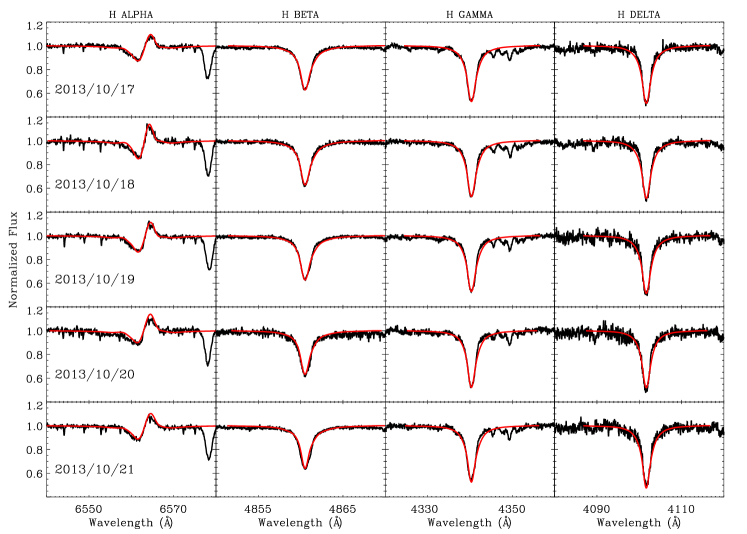
Figure 3: Sequence of fits to daily line variations of H and He lines in 2013. Fits to the different line transitions are achieved using individual values of $\varv_{\rm{mic}}$ and $\varv_{\rm{mac}}$ (for details see Sect. 4.1.3).

Figure 3: Continued.

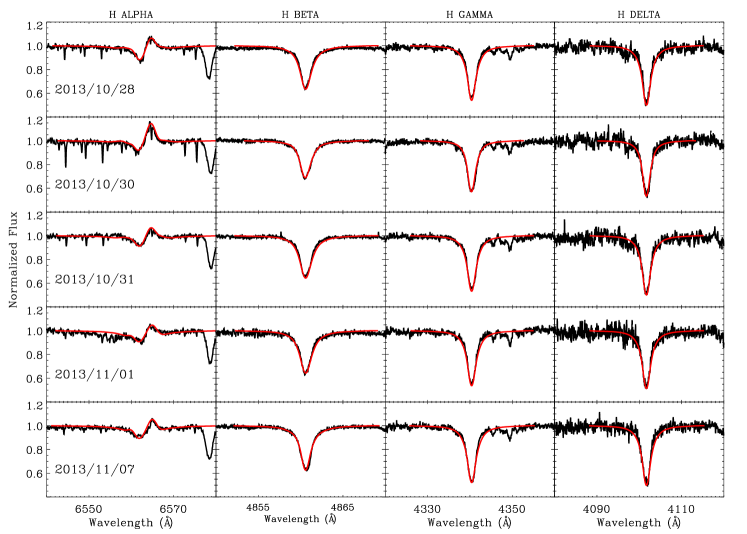
Figure 3: Continued.

Figure 4: H$\alpha$ line profiles taken in 2009 and 2010 at Ondřejov Observatory together with their corresponding model fits (for details see Table 2). Lines with highly complex profiles or roughly zero EW have not been fitted.

Figure 5: Same as Fig. 4, but for data taken in 2011.

Figure 6: Same as Fig. 4, but for data taken in 2012 (top) and 2013 (bottom).

4.1.1 Stellar parameters

On average, we represent the photosphere of the star with $T_{\rm{eff}}=18\,800$ K, with variations ranging from 18 570 K to 19 100 K (see Tables 1 and 2). We find a mean value for $\log\,g$ of 2.43 with a scatter of $\pm$0.14 dex, based on the fits of the H$\gamma$ line profile. The same trend is obtained from the Ondřejov spectra based on the analysis of the H$\alpha$ line alone. Although these latter $\log\,g$ values can be less accurate, they range from 2.3 to 2.5 dex, but their average is the same ($2.43\pm 0.1$ dex) as the mean value determined from the Arizona spectra. Both results predict marginally higher $\log\,g$ values than those previously reported in the literature ($\log\,g=2.2\pm 0.1$), which are typically based on only one or two measurements, but the agreement within the error bars is fairly good.

From the 15 Arizona spectra we obtain an average radius of $57\,R_{\odot}$ with a statistical dispersion of $\pm 1\,R_{\odot}$. This radius is close to the initial input value of $61\,R_{\odot}$. We noticed that changes in $\Delta R_{*}$ by more than $1\,R_{\odot}$ result in appreciable changes in the computed profiles. Moreover, several of the 43 H$\alpha$ profiles in the Ondřejov spectra (spread over four years) could not be modeled with a fixed radius of $57\pm 1\,R_{\odot}$. Instead, best-fit models were obtained for values ranging from $52\,R_{\odot}$ to $65\,R_{\odot}$. This suggests that the star either has a variable wind opacity or undergoes real radial changes, for example, via radial pulsations.

Using the mean value for R_⋆ and the surface gravity corrected for rotation, $\log\,g_{\rm true}=2.44\,$dex, we determine a stellar mass of $34\pm 4$ M_⊙. The mean stellar luminosity is found to be $\log L/$L${}_{\odot}=(5.57\pm 0.03)$, which agrees with values derived from observations.

Figure 7: Fits to the lines of Si ii $\lambda\lambda$ 4128, 4130 Å, and Si iii $\lambda$ 4552 Å  in the Arizona spectra. Fits to the different line transitions are achieved using individual values of $\varv_{\rm{mic}}$ and $\varv_{\rm{mac}}$ (for details see Sect. 4.1.3).

Table 1: Stellar and wind parameters obtained from line profile fits of observations taken in Arizona in 2013. Listed are the date of observation, the Julian date (JD), the derived effective temperature ($T_{\rm{eff}}$) and $\log\,g$, the $\beta$ exponent of the velocity law, the mass-loss rate ($\dot{M}$), the terminal velocity ($v_{\infty}$), the macroturbulent velocity in H$\alpha$ ($v_{\rm{macro}}$(H$\alpha$)), the stellar radius ($R_{\star}$), and the luminosity ($L$). Mass-loss rates are for smooth wind models.

Date	JD	$T_{\rm{eff}}$	$\log\,g$	$\beta$	$\dot{M}$	$v_{\infty}$	$v_{\rm{macro}}$(H$\alpha$)	$R_{\star}$	$\log\,L/L_{\odot}$
dd/mm/yr		[K]	[cgs]		[$10^{-6}$ $M_{\odot}$ yr-1]	[km s-1]	[km s-1]	[$R_{\odot}$]
17/10/2013	2 456 582.72	19 000$\pm 400$	2.50$\pm 0.1$	2.0	0.295$\pm 0.01$	310$\pm 30$	50$\pm 5$	58$\pm 1$	5.60$\pm 0.03$
18/10/2013	2 456 583.70	19 000$\pm 400$	2.50$\pm 0.1$	2.0	0.295$\pm 0.01$	310$\pm 30$	20$\pm 5$	58$\pm 1$	5.60$\pm 0.03$
19/10/2013	2 456 584.62	19 000$\pm 400$	2.50$\pm 0.1$	2.0	0.310$\pm 0.01$	320$\pm 30$	35$\pm 5$	58$\pm 1$	5.60$\pm 0.03$
20/10/2013	2 456 585.67	19 000$\pm 400$	2.47$\pm 0.1$	2.0	0.320$\pm 0.01$	320$\pm 30$	50$\pm 5$	57$\pm 1$	5.59$\pm 0.03$
21/10/2013	2 456 586.73	19 100$\pm 400$	2.50$\pm 0.1$	2.0	0.280$\pm 0.01$	300$\pm 30$	60$\pm 5$	57$\pm 1$	5.60$\pm 0.03$
22/10/2013	2 456 587.70	19 000$\pm 400$	2.40$\pm 0.1$	2.0	0.285$\pm 0.01$	310$\pm 30$	60$\pm 5$	58$\pm 1$	5.60$\pm 0.03$
23/10/2013	2 456 588.59	19 000$\pm 400$	2.40$\pm 0.1$	2.0	0.285$\pm 0.01$	350$\pm 35$	60$\pm 5$	58$\pm 1$	5.57$\pm 0.03$
25/10/2013	2 456 590.59	18 650$\pm 400$	2.40$\pm 0.1$	2.0	0.190$\pm 0.01$	300$\pm 30$	40$\pm 5$	58$\pm 1$	5.57$\pm 0.03$
26/10/2013	2 456 591.59	18 600$\pm 400$	2.40$\pm 0.1$	2.0	0.180$\pm 0.01$	270$\pm 30$	50$\pm 5$	57$\pm 1$	5.55$\pm 0.03$
27/10/2013	2 456 592.59	18 570$\pm 400$	2.40$\pm 0.1$	2.0	0.170$\pm 0.01$	270$\pm 30$	50$\pm 5$	56$\pm 1$	5.53$\pm 0.03$
28/10/2013	2 456 593.60	18 570$\pm 400$	2.40$\pm 0.1$	2.0	0.170$\pm 0.01$	270$\pm 30$	40$\pm 5$	56$\pm 1$	5.53$\pm 0.03$
30/10/2013	2 456 595.71	19 000$\pm 400$	2.36$\pm 0.1$	2.2	0.284$\pm 0.01$	330$\pm 30$	40$\pm 5$	57$\pm 1$	5.58$\pm 0.03$
31/10/2013	2 456 596.71	18 600$\pm 400$	2.40$\pm 0.1$	2.0	0.180$\pm 0.01$	270$\pm 30$	60$\pm 5$	57$\pm 1$	5.55$\pm 0.03$
01/11/2013	2 456 597.57	18 600$\pm 400$	2.40$\pm 0.1$	2.0	0.175$\pm 0.01$	260$\pm 30$	60$\pm 5$	57$\pm 1$	5.55$\pm 0.03$
07/11/2013	2 456 603.59	18 570$\pm 400$	2.40$\pm 0.1$	2.0	0.170$\pm 0.01$	270$\pm 30$	40$\pm 5$	56$\pm 1$	5.53$\pm 0.03$

Table 2: As Table 1, but for the observations taken in Ondřejov between 2009 and 2013.

Date	JD	$T_{\rm{eff}}$	$\log\,g$	$\beta$	$\dot{M}$	$v_{\infty}$	$v_{\rm{macro}}$(H$\alpha$)	$R_{\star}$	$\log\,L/L_{\odot}$
dd/mm/yr		[K]	[cgs]		[$10^{-6}$ $M_{\odot}$ yr-1]	[km s-1]	[km s-1]	[$R_{\odot}$]
15/08/2009	2455059.44	19000$\pm 1000$	2.40$\pm 0.1$	2.0	0.290$\pm 0.01$	310$\pm 30$	35$\pm 5$	58$\pm 2$	5.60$\pm$0.03
18/08/2009	2455062.43	19000$\pm 1000$	2.43$\pm 0.1$	2.0	0.295$\pm 0.01$	340$\pm 35$	50$\pm 5$	54$\pm 2$	5.54$\pm$0.03
23/08/2009	2455067.49	19000$\pm 1000$	2.43$\pm 0.1$	2.0	0.340$\pm 0.01$	320$\pm 30$	30$\pm 5$	55$\pm 2$	5.55$\pm$0.03
16/07/2010	2455394.41	18700$\pm 1000$	2.35$\pm 0.1$	2.0	0.240$\pm 0.01$	250$\pm 25$	14$\pm 5$	63$\pm 2$	5.64$\pm$0.03
31A/07/2010	2455409.37	18700$\pm 1000$	2.50$\pm 0.1$	2.0	0.195$\pm 0.01$	250$\pm 25$	35$\pm 5$	57$\pm 2$	5.56$\pm$0.03
31B/07/2010	2455409.53	18700$\pm 1000$	2.50$\pm 0.1$	2.0	0.195$\pm 0.01$	250$\pm 25$	40$\pm 5$	57$\pm 2$	5.56$\pm$0.03
01A/08/2010	2455410.35	18700$\pm 1000$	2.50$\pm 0.1$	2.0	0.195$\pm 0.02$	250$\pm 50$	80$\pm 10$	57$\pm 3$	5.56$\pm$0.06
01B/08/2010	2455410.41	18700$\pm 1000$	2.50$\pm 0.1$	2.0	0.195$\pm 0.02$	250$\pm 50$	90$\pm 10$	57$\pm 3$	5.56$\pm$0.06
01C/08/2010	2455410.45	18700$\pm 1000$	2.50$\pm 0.1$	2.0	0.195$\pm 0.02$	250$\pm 50$	100$\pm 10$	57$\pm 3$	5.56$\pm$0.06
04A/09/2010	2455444.38	18650$\pm 1000$	2.50$\pm 0.1$	2.0	0.175$\pm 0.01$	270$\pm 30$	20$\pm 5$	56$\pm 2$	5.54$\pm$0.03
04B/09/2010	2455444.41	18650$\pm 1000$	2.50$\pm 0.1$	2.0	0.175$\pm 0.01$	270$\pm 30$	30$\pm 5$	56$\pm 2$	5.54$\pm$0.03
04C/09/2010	2455444.45	18650$\pm 1000$	2.50$\pm 0.1$	2.0	0.175$\pm 0.01$	270$\pm 30$	40$\pm 5$	56$\pm 2$	5.54$\pm$0.03
05/09/2010	2455445.31	19000$\pm 1000$	2.41$\pm 0.1$	2.2	0.280$\pm 0.01$	310$\pm 30$	50$\pm 5$	55$\pm 2$	5.55 $\pm$0.03
06/09/2010	2455446.52	19000$\pm 1000$	2.41$\pm 0.1$	2.2	0.280$\pm 0.01$	310$\pm 30$	60$\pm 5$	55$\pm 2$	5.55$\pm$0.03
11/09/2010	2455451.27	18600$\pm 1000$	2.50$\pm 0.1$	2.0	0.195$\pm 0.01$	250$\pm 25$	120$\pm 10$	57$\pm 2$	5.55$\pm$0.03
21/09/2010	2455461.34	18600$\pm 1000$	2.40$\pm 0.1$	2.0	0.180$\pm 0.02$	250$\pm 50$	30$\pm 5$	58$\pm 3$	5.56$\pm$0.06
22/09/2010	2455462.32	18600$\pm 1000$	2.48$\pm 0.1$	2.0	0.153$\pm 0.02$	235$\pm 50$	55$\pm 5$	58$\pm 3$	5.64$\pm$0.06
23/09/2010	2455463.38	18700$\pm 1000$	2.42$\pm 0.1$	2.0	0.236$\pm 0.01$	260$\pm 25$	50$\pm 5$	63$\pm 2$	5.56$\pm$0.03
24/09/2010	2455464.38	19000$\pm 1000$	2.45$\pm 0.1$	2.0	0.305$\pm 0.01$	330$\pm 35$	35$\pm 5$	54$\pm 2$	5.54$\pm$0.03
06/03/2011	2455627.64	19000$\pm 1000$	2.43$\pm 0.1$	2.0	0.335$\pm 0.01$	320$\pm 30$	30$\pm 5$	55$\pm 2$	5.55$\pm$0.03
08/03/2011	2455629.60	19000$\pm 1000$	2.43$\pm 0.1$	2.0	0.360$\pm 0.01$	320$\pm 30$	20$\pm 5$	55$\pm 2$	5.55$\pm$0.03
19/03/2011	2455640.63	19000$\pm 1000$	2.43$\pm 0.1$	2.0	0.370$\pm 0.01$	320$\pm 30$	100$\pm 10$	55$\pm 2$	5.57$\pm$0.03
06/09/2011	2455811.40	18700$\pm 1000$	2.46$\pm 0.1$	2.0	0.265$\pm 0.01$	300$\pm 30$	30$\pm 5$	58$\pm 2$	5.58$\pm$0.03
25/09/2011	2455830.41	18900$\pm 1000$	2.45$\pm 0.1$	2.0	0.400$\pm 0.01$	700$\pm 70$	40$\pm 5$	55$\pm 2$	5.55$\pm$0.03
16/10/2011	2455851.38	19100$\pm 1000$	2.50$\pm 0.1$	2.0	0.238$\pm 0.01$	350$\pm 35$	50$\pm 5$	53$\pm 2$	5.53$\pm$0.03
26/02/2012	2455984.63	19000$\pm 1000$	2.50$\pm 0.1$	2.0	0.460$\pm 0.01$	600$\pm 60$	30$\pm 5$	52$\pm 2$	5.50$\pm$0.03
30/09/2012	2456201.23	18600$\pm 1000$	2.30$\pm 0.1$	2.0	0.210$\pm 0.01$	230$\pm 25$	80$\pm 10$	65$\pm 2$	5.67$\pm$0.03
03/10/2012	2456204.26	18600$\pm 1000$	2.30$\pm 0.1$	2.0	0.200$\pm 0.02$	230$\pm 50$	30$\pm 5$	65$\pm 3$	5.67$\pm$0.06
14/10/2012	2456215.28	19000$\pm 1000$	2.43$\pm 0.1$	2.0	0.293$\pm 0.01$	340$\pm 35$	30$\pm 5$	54$\pm 2$	5.54$\pm$0.03
14/11/2012	2456246.24	19100$\pm 1000$	2.46$\pm 0.1$	2.0	0.200$\pm 0.02$	450$\pm 90$	70$\pm 5$	58$\pm 3$	5.61$\pm$0.06
16/03/2013	2456368.52	19000$\pm 1000$	2.45$\pm 0.1$	2.0	0.300$\pm 0.01$	300$\pm 30$	40$\pm 5$	52$\pm 2$	5.51$\pm$0.03
21/04/2013	2456404.47	19000$\pm 1000$	2.45$\pm 0.1$	2.0	0.305$\pm 0.01$	330$\pm 35$	40$\pm 5$	54$\pm 2$	5.54$\pm$0.03
25/04/2013	2456408.47	19000$\pm 1000$	2.45$\pm 0.1$	2.0	0.305$\pm 0.01$	330$\pm 35$	30$\pm 5$	54$\pm 2$	5.54$\pm$0.03
19/07/2013	2456493.37	19000$\pm 1000$	2.40$\pm 0.1$	2.0	0.295$\pm 0.01$	310$\pm 30$	35$\pm 5$	58$\pm 2$	5.60$\pm$0.03
20/07/2013	2456494.35	18700$\pm 1000$	2.35$\pm 0.1$	2.0	0.200$\pm 0.01$	250$\pm 25$	50$\pm 5$	63$\pm 2$	5.65$\pm$0.03
21/07/2013	2456495.33	18700$\pm 1000$	2.35$\pm 0.1$	2.0	0.200$\pm 0.01$	250$\pm 25$	65$\pm 5$	63$\pm 2$	5.65$\pm$0.03
22/07/2013	2456496.35	18700$\pm 1000$	2.35$\pm 0.1$	2.0	0.200$\pm 0.01$	250$\pm 25$	110$\pm 10$	63$\pm 2$	5.65$\pm$0.03
23/07/2013	2456497.52	18700$\pm 1000$	2.35$\pm 0.1$	2.0	0.200$\pm 0.01$	250$\pm 25$	80$\pm 10$	63$\pm 2$	5.65$\pm$0.03
25/07/2013	2456499.55	18700$\pm 1000$	2.35$\pm 0.1$	2.0	0.200$\pm 0.02$	250$\pm 50$	150$\pm 15$	63$\pm 3$	5.65$\pm$0.06
30/07/2013	2456504.35	18700$\pm 1000$	2.35$\pm 0.1$	2.0	0.200$\pm 0.01$	250$\pm 25$	55$\pm 5$	63$\pm 2$	5.65$\pm$0.03
01/08/2013	2456506.57	18700$\pm 1000$	2.40$\pm 0.1$	1.6	0.215$\pm 0.01$	250$\pm 25$	40$\pm 5$	60$\pm 2$	5.60$\pm 0.03$
02/08/2013	2456507.34	19000$\pm 1000$	2.43$\pm 0.1$	2.0	0.295$\pm 0.01$	340$\pm 35$	80$\pm 10$	54$\pm 2$	5.54$\pm 0.03$
03/08/2013	2456508.34	19000$\pm 1000$	2.43$\pm 0.1$	2.0	0.295$\pm 0.01$	340$\pm 35$	70$\pm 5$	54$\pm 2$	5.54$\pm 0.03$

4.1.2 Wind variability

To gain insight into the variability of the stellar wind of 55 Cyg, we modeled the H$\alpha$ line profile over the observing period of about five years.

We fit the observations assuming a smooth (unclumped) wind structure represented by a $\beta$-velocity law, with $\beta=2.0$, except in rare cases, where the value of $\beta$ was slightly adjusted (1.6 and 2.2). On average, the derived $\dot{M}$ from the Ondřejov data is $\sim 2.5\times 10^{-7}$ M_⊙ yr^-1, with fluctuations of a factor of three between the minimum value of $1.5\times 10^{-7}$ M_⊙ yr^-1 and the maximum value of $4.6\times 10^{-7}$ M_⊙ yr^-1. Our results agree on average with the homogeneous wind parameters reported by Crowther et al. (2006): $\beta=2$ and $\dot{M}=2.3\times 10^{-7}$ M_⊙ yr^-1, and our values for the mass-loss fall between the extreme ones obtained for unclumped winds in the literature (see Sect. 2). In addition, the variation in the terminal velocity (ranging typically from 230 km s^-1 to 350 km s^-1) presents a positive correlation with the mass-loss rate. There are two exceptions with substantially higher values of 600 km s^-1 and 700 km s^-1, corresponding to the two occasions of highest mass loss of $4.6\times 10^{-7}$ M_⊙ yr^-1 and $4.0\times 10^{-7}$ M_⊙ yr^-1. The corresponding observations were taken on 2011 September 25 and 2012 February 26, when a mass eruptive event probably occurred. The terminal velocities found are higher than the 200 km s^-1 reported by Markova & Puls (2008) and lower than the 470 km s^-1 adopted by Crowther et al. (2006).

The average mass-loss rate obtained (Ondřejov observations) is consistent with the average $\dot{M}$ value estimated from the high-resolution spectra taken in Arizona during October and November, 2013. Furthermore, the Arizona spectra show changes in the intensity of the H$\alpha$ line (as shown in Fig. 3) and variations in the mass-loss rate by a factor of 1.9.

4.1.3 Turbulent and projected rotation velocities

In addition to the stellar and wind parameters discussed so far, three more parameters were used to match the observed line profiles. These are microturbulence, macroturbulence, and projected rotation velocity. Microturbulent velocities refer to atmospheric motions on scales below the photon mean free path, and there is evidence that these motions could result from subsurface convection caused by the iron opacity peak (Cantiello et al. 2009). The values found for BSGs range between 5 km s^-1 and 15 km s^-1 with a tendency to decrease with decreasing temperature (e.g., Markova & Puls 2008). Fits to the helium absorption lines give best results for $10\pm 2$ km s^-1, except for He i $\lambda$ 6678, which requires a higher value ($17\pm 2$ km s^-1). Similar values are observed in Si ii and Si iii lines, with $12\pm 2$ km s^-1 and $7\pm 2$ km s^-1, respectively. The line profiles of H$\alpha$ also require a higher microturbulent velocity to achieve satisfactory fits. Here, a value of $\sim 50\pm 5$ km s^-1 is needed, which can be explained by the fact that H$\alpha$ is formed in the lower wind where supersonic turbulent velocities can occur. Problems in fitting H$\alpha$ line profiles are not new, and, for many BSGs, values as high as 50 km s^-1 (or turbulent velocities increasing linearly from the photospheric value to about 50 km s^-1) were reported (e.g., Crowther et al. 2006; Searle et al. 2008). A possible interpretation of the greater microturbulent velocity value for He i $\lambda$ 6678 might be that the line-forming region extends into the base of the wind where it is affected by the wind turbulence. We return to this point in Sect. 5.2.

After including the microturbulence, the synthetic line profiles must be broadened by the combined effect of stellar rotation and macroturbulence. Considering that $v\sin i$, as a global parameter, should be the same for all lines, the variability in the line profiles must be assigned to macroturbulent broadening. For H and He I lines, the best fit was achieved with $v\sin i=55\pm 5$ km s^-1 (see also Sect. 5.2), but theoretical and observed Si ii and Si iii lines match better if $v\sin i$ is taken around $40\pm 5$ km s^-1 or $45\pm 5$ km s^-1. We also note that the macroturbulence can be quite different in various lines. For instance, from modeling the Arizona data, we found that $v_{\rm macro}$ is relatively small in the lines of He i $\lambda$ 4471 (6-7 km s^-1), He i $\lambda$ 4713 (11-12 km s^-1), and H$\delta$ (14-15 km s^-1), and approximately constant throughout the observing period. In H$\gamma$, the changes are larger (14-30 km s^-1). The situation changes for H$\beta$ and He i $\lambda$ 6678, for which much higher and strongly variable values are found (25-90 km s^-1 and 20-50 km s^-1, respectively). Those obtained for H$\alpha$ vary in the range 20-60 km s^-1 (see Table 1). The Si ii and Si iii lines also show a large dispersion in $v_{\rm macro}$, they range from 10 km s^-1 to 30 km s^-1, and 30 km s^-1 to 50 km s^-1, respectively, with uncertanties of $\pm$ 5 km s^-1.

The data from Ondřejov provide macroturbulent velocities only for H$\alpha$ and He i $\lambda$ 6678 Å.  Over the entire observing period, we obtain values in the range 30-60 km s^-1 for He i $\lambda$ 6678 Å,  while for H$\alpha$, occasionally values of more than 100 km s^-1 are found (see Table 2). In most spectra, we find that for both lines the contribution of macroturbulence to the line broadening is comparable to or higher than that from $v\sin i$. Such high values are commonly found in BSGs (e.g., Ryans et al. 2002; Simón-Díaz & Herrero 2007; Markova & Puls 2008; Markova et al. 2014; Simón-Díaz & Herrero 2014), and the values of $v\sin i$ and $v_{\rm macro}$ found for 55 Cyg agree well with those of BSGs of comparable mass and effective temperature (see Markova et al. 2014).

Figure 8: Top panel: Variation of the H$\alpha$ line for different He abundances: $N$(He)/$N$(H) = 0.1 (solid line), $N$(He)/$N$(H) = 0.2 (dotted line), and $N$(He)/$N$(H) = 0.4 (dashed line) and the same mass-loss rate. Bottom panel: Similar H$\alpha$ line profiles derived using the same $N$(He)/$N$(H) ratios, as in the previous plot, but with different mass-loss rates: $1.9\times 10^{-7}$ M_⊙ yr^-1 (solid line), $2.5\times 10^{-7}$ M_⊙ yr^-1 (dotted line), and $3.5\times 10^{-7}$ M_⊙ yr^-1 (dashed line).

Figure 9: Variation of the He i lines computed for a rotating star ($V\,\sin\,i$ = 60 km s^-1) with He contents of $N(He)/N(H)$= 0.1 (solid line), $N(He)/N(H)$= 0.2 (dotted line) and $N(He)/N(H)$= 0.4 (dashed line). The intensity of the He i forbidden components at $\lambda$ 4470 and $\lambda$ 4922 serves as an ideal indicator for the He abundance.

4.1.4 Atmospheric chemical composition

The H$\alpha$ line is known to be sensitive to variations in the He content, in the sense that He-rich wind models produce H$\alpha$ EWs that are a factor of 2-3 lower than those with solar He abundance (Petrov et al. 2014). As the mass-loss rate is a function of metallicity and is derived from the strength of the H$\alpha$ line, we expect a lack of uniqueness in wind models, which are based purely on the modeling of H transitions.

This ambiguity is demonstrated in Fig. 8, where we show in the top panel the H$\alpha$ line computed for a constant mass-loss rate of $1.9\times 10^{-7}$ M_⊙ yr^-1 and $N$(He)/$N$(H) ratios of 0.1, 0.2, and 0.4. To compensate for the vanishing H$\alpha$ emission with increasing He abundance, we must increase the mass-loss rate to $2.5\times 10^{-7}$ M_⊙ yr^-1 and $3.5\times 10^{-7}$ M_⊙ yr^-1, respectively. Then all three models produce approximately identical H$\alpha$ profiles (bottom panel of Fig. 8). Consequently, uncertainties in the chemical composition (here He abundance) by a factor of 2–4 may affect the derived mass-loss rate by a factor of 1.3–1.9.

However, a higher He abundance also sensitively alters the strength of both the permitted and forbidden components of the He lines (see Fig. 9). When increasing the He abundance for a fixed mass-loss rate, the forbidden components develop prominent absorption features in the wings of the permitted lines. These manifest as pronounced asymmetries in the profiles of the permitted components, even if the projected rotational velocity is as high as $\sim 60$ km s^-1. The presence and strength of the forbidden component hence serve as useful diagnostics for the He surface abundance of slowly rotating stars.

As the He line profiles observed in 55 Cyg do not show noticeable contributions from the forbidden components, a solar He abundance was found to be more appropriate to fit both the H$\alpha$ and He lines.

In relation to the modeling of the Si ii and Si iii lines, we were able to obtain good fits using solar abundance, but the question remains of how sensitive the Si lines are to changes in their content. The influence of non-solar abundance on $T_{\rm eff}$ was discussed in detail by Lefever et al. (2007) and Markova & Puls (2008), who found that higher abundances result in lower $T_{\rm eff}$ values and vice versa. Such a change in temperature ($\Delta T_{\rm eff}>1\,000$ K) would also affect the He lines. However, from our model fits, we do not find a discrepancy between the temperature obtained from the He and the Si lines. Therefore, the assumption of solar abundance for Si (within a range $\pm 0.15$ dex) is well justified. All other elements are treated as background elements with solar abundance.

Figure 10: Variation in the first moment (radial velocity, without correction for systemic velocity) of the He i $\lambda$ 6678 Å  line in the period August 2009 to October 2013.

4.2 Searching for pulsations

As 55 Cyg resides inside the instability domain for BSGs (Saio et al. 2006) and $\alpha$ Cygni variables (Saio et al. 2013), it is natural to assume that pulsations might also be at work on the surface of this star. The strong variability in the H$\alpha$ line (suggesting variable mass-loss) could indicate that the observed changes in the wind might be connected to pulsations detectable in photospheric line variations. To test this hypothesis, this section is devoted to a detailed variability analysis of photospheric line profiles.

4.2.1 Photospheric line profile variability

In the absence of long-term photometric light curves, the presence of pulsations can also be tested by analyzing the variability of photospheric lines in high-quality optical spectra. The spectral range observed with the Perek 2m telescope contains several photospheric lines (see Fig. 1); the strongest is He i $\lambda$6678 Å, followed by the deep absorption lines of C ii $\lambda\lambda$ 6578, 6583 Å.  Considerably weaker lines of Si ii $\lambda\lambda$ 6347, 6371 Å,  Ne i $\lambda\lambda$ 6402, 6507 Å,  and N ii $\lambda\lambda$ 6482, 6611 Å are present as well. Despite the presence of these metal lines, we restricted most of our analysis to He i for two reasons. First, this line is not affected by telluric features, contrary to other lines such as H$\alpha$, C ii $\lambda\lambda$ 6578, 6583 Å,  Si ii $\lambda\lambda$ 6347, 6371 Å,  and N ii $\lambda\lambda$ 6482, 6611 Å.  Any correction of the spectra with a telluric spectrum obtained from observing a standard star superimposes additional noise to the continuum level of the science spectra. Because He i $\lambda$ 6678 Å falls outside regions of telluric pollution, no cleaning is required, and the initial quality of the spectral line is preserved. Second, while only the C ii lines are sufficiently strong for an analysis without suffering from an enhanced continuum noise level, these lines arise within a broad and shallow emission component centered on H$\alpha$ (see Fig. 1). The shape of the line profiles of these C ii lines can thus be (possibly severely) altered by the normalization process, imprinting additional errors. These metal lines are, therefore, less favorable for the analysis of reliable line profile variabilities, but can be used as a secondary criterion to prove pulsation activity.

Figure 11: Variation in EW (top), first (radial velocity, middle), and third moment (skewness, bottom) of He i $\lambda$ 6678 Å  in the observing period 2013 July 19 to August 12.

4.2.2 Moment analyses

For further analysis, we excluded all spectra that have exposure times longer than 1800 s. This leaves us with a total of 325 spectra, most with exposure times between 400 s and 900 s.

To search for line profile variabilities in He i $\lambda$ 6678 Å, we applied the moment method (Aerts et al. 1992; North & Paltani 1994). This method is ideal, as it allows distinguishing between line profile variability caused by stellar spots or pulsations. We computed the first three moments of He i $\lambda$ 6678 Å  using the prescription of Aerts et al. (1992). The first moment corresponds to the radial velocity. This parameter varies between +5 km s^-1 and -21 km s^-1 over the total observing period from August 2009 to October 2013 (see Fig. 10). The offset from a symmetric variation around zero velocity is caused by the star’s intrinsic radial velocity, which we determine from this plot to be $\varv_{\rm rad,star}\simeq-8$ km s^-1. We corrected the data for this stellar motion before we continued with our analysis. Hence, the observed maximum amplitude of the radial velocity variation in the line profile is about $\pm 13$ km s^-1.

Figure 12: Variation in the first moment (radial velocity) of He i $\lambda$ 6678 Å  (dots), C ii $\lambda$ 6578 Å  (squares), and Si ii $\lambda$ 6347 Å  (triangles) during the nights 2013 July 21-22.

Table 3: 55 Cyg periodicities

No.	$f$	$df\times 10^{8}$	$A$	$dA$	$\Phi$	$d\Phi$
	(day-1)		(km s-1)		(rad)
$f_{1}$	0.044366	0.03	4.39	0.03	2.43	0.01
$f_{2}$	0.995570	0.03	3.31	0.04	3.71	0.02
$f_{3}$	0.235716	0.07	2.54	0.03	3.44	0.06
$f_{4}$	0.974983	0.17	1.42	0.03	5.40	0.09
$f_{5}$	1.278593	0.18	1.37	0.03	3.35	0.10
$f_{6}$	2.400132	0.17	1.54	0.02	1.21	0.11
$f_{7}$	0.506733	0.22	1.30	0.07	5.55	0.13
$f_{8}$	4.163120	0.26	0.87	0.01	5.78	0.17
$f_{9}$	6.994100	0.21	0.95	0.01	1.76	0.14
$f_{10}$	3.104664	0.18	1.18	0.02	5.29	0.10
$f_{11}$	0.188665	0.42	1.09	0.04	3.43	0.26
$f_{12}$	1.462843	0.40	1.06	0.03	2.77	0.25
$f_{13}$	0.296804	0.24	1.11	0.03	3.31	0.14
$f_{14}$	0.652575	1.21	0.79	0.03	1.24	0.77
$f_{15}$	1.181013	1.55	0.55	0.04	6.03	1.00
$f_{16}$	0.617903	0.30	1.00	0.02	0.04	0.17
$f_{17}$	2.593881	0.45	0.75	0.02	5.46	0.28
$f_{18}$	9.003491	0.52	0.54	0.01	2.09	0.34
$f_{19}$	3.780456	1.10	0.51	0.02	4.94	0.79

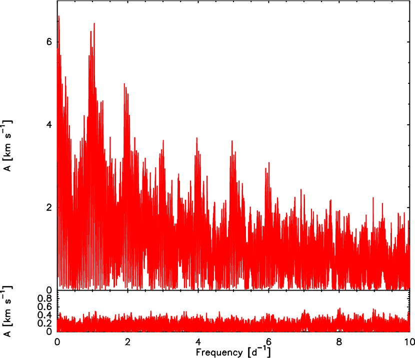
Figure 13: Lomb-Scargle periodogram of the original radial velocity data (top) and of the data cleaned with the identified 19 sinusoids (bottom).

Next, we compared the behavior of the first and third moments. Their time variability is shown in the middle and bottom panels of Fig. 11. For better visibility and clarity, the plot is limited to a period of 25 days, ranging from 2013 July 19 to August 12. This period contains time-series within seven nights, four at the beginning and three at the end. Obviously, the third moment, which describes the skewness (i.e., the asymmetry) of the line profile displays a strong time variability. In addition, the third moment varies in phase with the radial velocity, which is characteristic for stellar pulsations (see, e.g., Aerts et al. 1992). Similar behavior is seen in other seasons.

Additional proof for pulsation activity in the atmosphere of 55 Cyg is provided by comparing moments from different elements. Although, as mentioned above, the other lines in the spectrum have a lower quality, we computed the moments of the lines C ii $\lambda$ 6578 Å  and Si ii $\lambda$ 6347 Å , but restricted to the time-series obtained during the nights 2013 July 21-22, which have the highest S/N. The results for the first moment of these lines compared to He i $\lambda$ 6678 Å  are shown in Fig. 12. Obviously, all three lines vary identically. Such a behavior excludes the possibility of stellar spots. If the star has a patchy surface abundance pattern, as is common in chemically peculiar stars, for instance, the radial velocities of the He lines vary typically differently from those of the metal lines (e.g., Briquet et al. 2001, 2004; Lehmann et al. 2006). Instead, the identical variability of the line profiles of both He and metals in 55 Cyg is very typical for pulsations.

The clear offset of the radial velocity curves of different lines could indicate that a velocity gradient exists within the atmosphere of 55 Cyg. In addition, the Si ii $\lambda$ 6347 Å line, which is the weakest of these three, displays negative velocities, but the acceleration is in phase with the other two lines that display positive velocitites. Unfortunately, the resolution of our spectra is too low to perform proper mode identification, so that no clear statements about the nature of the pulsations (radial, non-radial) can be made.

Figure 14: Fit (solid line) to the radial velocity variations (dots) of 55 Cyg in the total period 2013 July 19 to August 12 (top) and zoomed in for the two marked series (bottom).

4.2.3 Frequency analysis

The results from the moment analysis suggest pulsations as the most plausible cause for the observed line profile variability in He, as well as in the metal lines. The clear next step is to analyze the radial velocity curve to search for periods. We performed a frequency analysis using a similar strategy as the one described by Saio et al. (2006). We first computed a Lomb-Scargle periodogram (Scargle 1982) for frequency identification and amplitude estimation, which is displayed in the top panel of Fig. 13. The periodogram finds no single dominant period. Instead, it seems that multiple significant peaks are present. Such a behavior is known for the $\alpha$ Cygni variables (Lucy 1976), for instance, and has also been reported for the periodograms of other BSGs (e.g., Saio et al. 2006), and we therefore used a fitting function consisting of a series of sinusoids. To refine the parameters for the identified frequency, we applied a nonlinear least-squares fit. A sine curve was fit to the data and subtracted. Then we searched for the next frequency within the residuals. In each subsequent cycle, the sum of all previously identified sine curves was subtracted from the original data. The procedure was stopped as soon as the S/N of the next frequency was too low.

We define the noise level $\sigma_{\rm res}$ as the mean amplitude of the residual in a frequency interval around the identified frequency. The noise level in the frequency range 0 to 10 cycles day^-1 is 0.13 km s^-1. Frequencies with an amplitude $A>4\sigma_{\rm res}$ correspond to a confidence level of 99.9%, and are considered as clear detections. Those with $A>3.6\sigma_{\rm res}$ correspond to a confidence level of 95%. In total, we identified 19 frequencies. Only the last one has an amplitude of $3.7\sigma_{\rm res}$, and should thus be considered as less accurate. All other detections have amplitudes $A>4\sigma_{\rm res}$.

Figure 15: Variation in EW (top) of the He i $\lambda$ 6678 Å  line over the total observing period, the radial velocity (middle) and the residuals of the radial velocity (bottom) after pre-whitening with the superposition of 19 sinusoids.

Figure 16: Radial velocity and EW of the H i $\lambda$6678 line phased to the longest period (22.5 d). The corresponding sine curve with the parameters from Table 3 is included in the phase diagram of the radial velocity, and a tentative fit to the EW, which reveals the same period but is phase-shifted.

With all frequencies identified, we again performed a least-squares fit using the parameters of all periods as first-guess values. The final refined parameters of each sine curve with their errors are listed in Table 3. The Lomb-Scargle periodogram of the data, pre-whitened with the 19 identified periodicities, is shown in the bottom panel of Fig. 13.

Next, we computed the sum of the 19 individual sinusoids as a function of time (i.e., HJD) and compared it to the observations. The synthetic radial velocity curve looks rather chaotic. For clarity and better visibility, we plot the synthetic curve limited to a period of 25 days in the top panel of Fig. 14 and overplot the values obtained from the observations. In this plot, we mark two series, which correspond to the time interval where we obtained time series of observations of four and three consecutive nights. The comparison between the model and the observations of these series is shown, zoomed in, in the bottom panels of Fig. 14.

In addition to the radial velocity of the He i $\lambda$6678 line, we also computed the line EW. Its value over the complete four-year observing period is displayed in the top panel of Fig. 15. It is found to be quite variable as well, which is an indication for temperature variations in the stellar atmosphere (e.g., De Ridder et al. 2002). We phased the data (both EW and first moment) to the longest period of 22.5 days identified from the radial velocity curve. This phase diagram is shown in Fig. 16. The radial velocity clearly displays a sinusoidal behavior (bottom panel, with the sine curve of the identified period overplotted). We reveal variability with the same period in EW (top panel), but with a phase shift of $94\degr$. Considering that this period could belong to a radial (strange) mode, a phase shift in EW of $90\degr$ would imply an adiabatic pulsation mode, while slight deviations are usually interpreted as non-adiabatic effects. Moreover, the large scatter in the phased EW can be explained by the multiperiodicity (De Ridder et al. 2002).

5 Discussion

We interpret the spectroscopic variability observed in the blue supergiant star 55 Cyg in terms of photospheric oscillation modes and a time-variable radiation-driven wind. We discuss the reliability of the identified frequencies and the variation of wind parameter models. We also discuss the possibility that photospheric and wind variations might be related.

5.1 Reliability of the frequencies

The agreement between the synthetic radial velocity curve and the observations seems to be quite good (see Fig. 14), but not all data fall on the model curve. This is also visible from the final residuals, which still display some scatter. These residuals are shown for the full observing period in the bottom panel of Fig. 15, in comparison to the original observed radial velocity variation (middle panel).

There are three possible reasons why we did not obtain better fits to the radial velocity curve. First, the number of observations is not sufficient to properly determine the stellar radial velocity component. Hence, the data might not be exactly symmetric around zero, influencing the determination of the frequencies and amplitudes of the periods. Second, not all data points have the same high quality, and there are a number of rather large gaps in the observations. Both lead to an increase in the noise level of the amplitude spectrum. Hence, from ground-based spectroscopy we identify only 19 frequencies, while (many) more might be present. For comparison, 48 frequencies were identified in the supergiant HD 163 899 by Saio et al. (2006), using space-based photometry. Third, nothing is known about the stability of the periodic variations in 55 Cyg. As the observing period stretches over more than four years, some of the periodicities might have changed or completely disappeared, while others might have appeared. Such a behavior of flipping periodicities was reported by Markova et al. (2008) for the BSG star HD 199 478. Furthermore, Aerts et al. (2010b) recognized a sudden change in the amplitude of the pulsation mode in the BSG star HD 50 064.

Consequently, precise determinations of currently present periodicities in 55 Cyg must be obtained from a better dataset, ideally from continuous spectroscopic observations over a long time interval, combined with a continuous photometric light curve. This is a non-trivial task, however.

5.2 Stellar rotation

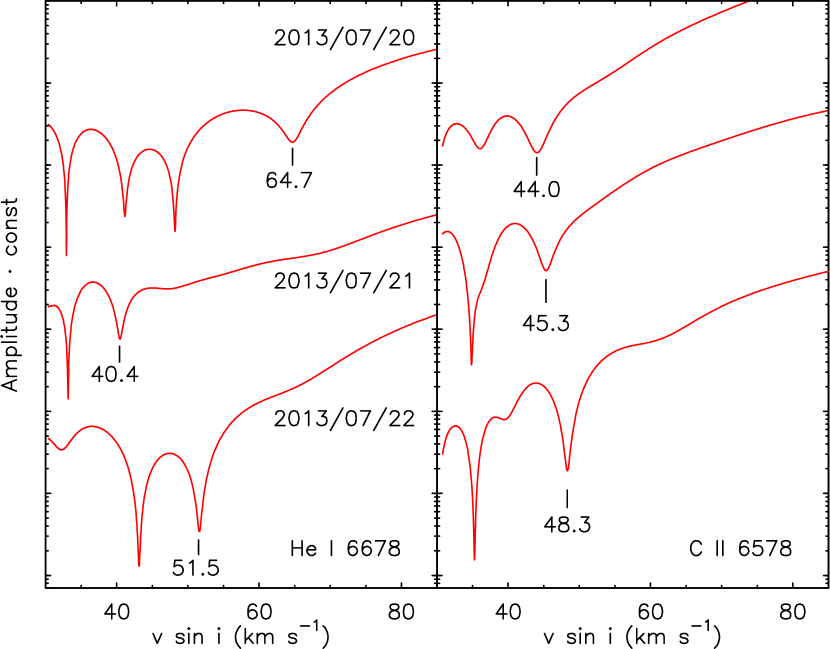
Figure 17: Top: Selection of values of $v\sin i$ obtained with the FT method for He i $\lambda$6678 Å  (left) and C ii $\lambda$6578 Å  (right) within the night of 2013 July 22. Only results with a clear first minimum are shown. Bottom: Range in $v\sin i$ values obtained within three consecutive nights.

The presence of multiple periodicities with significant velocity amplitudes in the photospheric lines implies that their profiles are affected in two ways. First, the lines can be expected to be broadened (referred to as macroturbulence) in excess of the typical broadening mechanisms acting in stellar atmospheres, including stellar rotation. And second, the profile shape is usually not symmetric anymore. The latter is confirmed from our moment analysis (see Fig. 11). However, the amounts of both rotation and macroturbulence are not known initially. The determination of proper stellar rotation rates is particularly important because rotation plays a major role in the evolution and mass-loss behavior of massive stars (see, e.g., Maeder & Meynet 2000; Meynet & Maeder 2005; Ekström et al. 2012; Simón-Díaz & Herrero 2014).

Investigations based on different methods, such as the Fourier transformation (FT) or the goodness-of-fit (GOF), are usually applied with the aim to determine proper $v\sin i$ values and the contribution of macroturbulence. However, a degeneracy exists, which allows fitting observed line profiles with a diversity of different combinations of $v\sin i$ and $v_{\rm macro}$ (e.g., Ryans et al. 2002). This degeneracy was also found for 55 Cyg by Jurkić et al. (2011) from modeling silicon lines in IUE spectra. Furthermore, the major requirement for a reliable result from the FT method is a symmetric signal. Application to asymmetric line profiles, as is typically expected for pulsating stars, immediately delivers false results. Studies of the effect of pulsational activity in stellar atmospheres on resulting line profiles revealed that the collective effect of multiple periodicities, for example, in the form of low-amplitude non-radial gravity modes, can cause substantial line broadening, which might be identified with macroturbulence (Aerts et al. 2009; Simón-Díaz et al. 2010a). These investigations also revealed that the FT method fails as soon as pulsations play a non-negligible role in the line width. Moreover, Aerts et al. (2014) showed that results from the FT of line profiles of known pulsators vary substantially over the pulsation cycle.

Even though our observations have extremely good S/N, which is considered as a major prerequisite for reliable results from the FT (Simón-Díaz & Herrero 2007), it is not possible to determine consistent $v\sin i$ values for 55 Cyg. This is shown in Fig. 17, where we plot the results from the FT analysis of He i $\lambda$6678 Å  and C ii $\lambda$6578 Å  during different times within one night (top panel) and extreme values obtained during three consecutive nights (bottom panel). For many line profiles (for both He i and C ii) the FT of our data deliver no clear minimum and, hence, no value for $v\sin i$ could be found.

From the profiles with clear zero points in their FT, C ii suggests $v\sin i$ values between 44 km s^-1 and 48 km s^-1 (which resemble the rotational values of 40 km s^-1 and 45 km s^-1 obtained for the Si ii lines). The values obtained from the He i line are in most cases significantly higher and with a higher spread in values, for example, from about 40 km s^-1 to about 65 km s^-1. While a shift in the position of the first zero point and the appearance of saddle points and local minima in the FT can be expected in the case of pulsations (Aerts et al. 2014), the discrepancy in the values obtained from the two investigated lines is difficult to understand as the FT method usually results in very similar $v\sin i$ values when applied to He and metal lines (Simón-Díaz & Herrero 2007). While the variation in values obtained from C ii is small, it may still imply that macroturbulent line broadening (and hence the underlying pulsations) influences the position of the zero points. In that context, strongly varying $v\sin i$ values within a single night were obtained from the FT method applied to the Si ii $\lambda$ 6347 line of the BSG HD 202 850 by Tomić et al. (2015).

In addition to the seemingly higher $v\sin i$ value resulting from the FT, the He i $\lambda$6678 Å line also appears to be special in other aspects. For instance, the measured radial velocity is higher than in the C ii $\lambda$6578 Å line (see Fig. 12). Moreover, He i $\lambda$6678 Å is the only line in our sample (apart from H$\alpha$) that requires substantially higher values for both the micro- and macroturbulent velocities than all other modeled photospheric lines. A possible explanation could be that the C ii $\lambda$6578 Å and the He i $\lambda$6678 Å lines are formed in different regions in the atmosphere with C ii originating in deeper layers, in agreement with the C ii line being much weaker than the He i line (see Fig. 1). The line-forming region for He i might be substantially larger and may be extending into the base of the wind, where higher turbulent velocities (i.e., higher than in the photosphere) might be expected due to instabilities, possibly resulting from coupling of the pulsation modes.

Although the FT analysis of the line profiles has severe problems in the presence of strong macroturbulence and possible wind contamination of the profiles, the range of values obtained from both lines is on the same order as the value of $55\pm 5$ km s^-1 found from the line profile fits (see Sect. 4.1.3). However, as long as the pulsation modes cannot be identified, the individual contributions from the two different, but physically very important mechanisms acting on the line profiles, that is, rotation and pulsations, remain uncertain.

5.3 Connection between pulsations and mass-loss

Our analysis revealed multiple periods, which can be interpreted as stellar pulsations. Hence, the question arises whether these pulsations might be suitable to trigger time-dependent enhanced mass loss, a question that was also addressed by Lefever et al. (2007) for a large sample of BSGs with no firm answer.

Two frequencies in the set of frequencies identified in Sect. 4.2.3, f₃ (4.2 days) and f₁₁ (5.3 days), are close to the spectroscopic period of 4–5 days reported by Granes (1975) and the periodicity of 4.88 days found in the photometric light curve by Koen & Eyer (2002). Twelve frequencies correspond to oscillations with periods spreading from $\sim 2.7$ hours to $\sim\,$24 hours. The frequencies f₅ and f₆ might be harmonics of f₁₅ and f₁₆, respectively. Meanwhile, the frequencies associated with periods of about one day (f₂ and f₄) might be related to the daily variations observed in the intensity of the H$\alpha$ line because their similar frequencies cause beats.

We would like to stress that the daily changes in line profile shape and intensity seen in our data should not be interpreted as a real change in mass loss. Each of our spectra has been modeled independently, considering a spherical smooth wind with a $\beta$ velocity law. However, any density enhancement at the base of the wind due to some mass ejection (triggered by pulsation or any other instability) will need time to travel through the H$\alpha$ line-forming region and hence contribute to the H$\alpha$ line profile in more than just one night. The night-to-night variations that we see in the data can therefore not be regarded as real changes in the wind parameters (mass loss and terminal velocity) but should rather be interpreted as rapid changes in the wind density, that is, wind inhomogeneities, traveling through the wind and influencing the H$\alpha$ line profile.

It is also worth mentioning that there were three occasions at which the H$\alpha$ line completely (or almost completely) disappeared from the spectrum, indicating that in these particular cases the wind emission was reduced so that it compensated by coincidence for the photospheric absorption line. The first time noted was on 2010 July 2-4 by Maharramov (2013), and in our own data we recognized it on 2012 July 24 and in 2013, around July 26. Interestingly, after the re-appearance of the H$\alpha$ in emission, its profile does not recover the shape seen before the cancellation. Instead, a strong, pure emission evolves during 2013 August 10-12, which might be explained as due to an enhanced amount of material appearing in the H$\alpha$ line-forming region. Furthermore, inspection of the behavior of the He i $\lambda$6678 line in the same period reveals a strong increase in the radial velocity (middle panel of Fig. 11) with a simultaneous drop in EW (top panel of Fig. 11).

If the occasions of annihilation of emission and absorption components of the H$\alpha$ line were periodic, the possible period would be on the order of about one year. We may speculate that the wind conditions of 55 Cyg may have changed some years ago, because no earlier observational work on 55 Cyg mentions phases in which the wind emission replenishes the photospheric absorption line.

On the other hand, according to the stellar parameters derived in this work, $\log\,L/L_{\odot}=5.57$, and the current stellar mass of 34 M_⊙, we find a ratio for $L/M\,\sim\,1.1\times 10^{4}$ L_⊙/M_⊙ , which is high enough for the occurrence of radial strange modes (Gautschy & Glatzel 1990; Glatzel 1994; Saio et al. 1998). The stellar properties of 55 Cyg resemble those of HD 50 064, for which Aerts et al. (2010b) argued that the star is building up a circumstellar envelope, as seen in the variable Balmer lines, while pulsating in a radial strange mode. A similar scenario might also hold for 55 Cyg. The first frequency, f₁ (22.5 days), has the proper length to be interpreted as radial strange mode as predicted from theory (Saio et al. 2013). This period might tentatively be connected to the mid-term variation observed in the H$\alpha$ line and the mass-loss rates. Considering the sequence of observations obtained in October 2013 in Arizona, it seems that the mass-loss rate may keep more or less a constant value over a time interval of roughly a week, followed by a jump to a lower mass-loss regime. This second regime might have lasted seven or perhaps more days (neglecting the sudden jump in the mass-loss observed on October, 30). Another period of at least five days of constant behavior can be recognized in July 2013. Whether this (quasi-)periodic variability in mass-loss might be recovered in other seasons cannot be asserted because of the often large gaps in observations.

Additional support for a possible connection between pulsations and enhanced mass loss is provided by the variable line shapes of H$\alpha$ and by the faint shallow symmetric wings extending to $\pm 1200$ km s^-1 (described in Sect. 3). The velocity of these wings is definitely higher than the wind terminal velocities determined for 55 Cyg, so that they are not formed by the current wind material. Instead, we interpret these wings as due to incoherent electron scattering in the outer layers of the star’s extended envelope above the line formation region. As the wings were not reported by other observers (with one exception, see Ebbets 1982), but are rather stable during the past four years, the pulsational activity leading to the formation of an optically thick, expanding atmosphere might have started or increased within the past few years.

5.4 Evolutionary state of 55 Cyg

According to the derived effective temperature and luminosity, we might connect the star with an evolutionary track of 40 M_⊙. The assignment of a proper evolutionary state of the star is hampered by the fact that massive stars can cross the temperature range of BSGs more than once during their evolution. The location of a star in the HRD alone is thus not sufficient, and additional criteria are needed for an unambiguous evolutionary state determination. One such criterion is provided by the recent calculations of the occurrence of possible pulsation modes during the post-main sequence evolution of massive stars by Saio et al. (2013). Their investigations revealed that during the post-RSG evolution, BSGs can pulsate in many more modes and, in particular, in radial strange modes, which is not possible while the star is on its first redward evolution. Moreover, the observations of pulsation properties with very many excited modes are possible only after the star has experienced a strong mass-loss during the RSG phase.

The numerous periodicities identified in 55 Cyg display a mixture of p- and g-modes. According to computations of pulsation modes in BSGs, for rotating stellar models in the range of initial masses of 20-25 M_⊙yr^-1 (Saio et al. 2006, 2013), the co-existence of both types of modes in the pre-RSG stage is found for stars with temperatures $T_{\rm{eff}}\ga 20\,000$ K, while cooler stars are expected to display very few pulsations. Even though the temperature of 55 Cyg, $T_{\rm{eff}}$ = 19 000 K, is slightly lower, its periodicities are too numerous to fit in a pre-RSG scenario. Consequently, a post-RSG stage is more plausible mainly because of the multiple pulsation modes (with periods $\la 30$ days) that we find in this star. Furthermore, the classification of 55 Cyg as a post-RSG is supported by the presence of the bow shock feature detected by the Wide-field Infrared Survey Explorer (WISE, Wright et al. 2010) in band 4 at 24 $\mu$m (see Fig. 18), which formed in the past by the interaction of a strong wind phase with the ISM.

But this post-RSG scenario does not seem to fit the low He surface abundance we derived from our line profile modeling. This apparent contradiction was also found in at least two other BSGs (Rigel and Deneb, see Saio et al. 2013). To solve this problem, Georgy et al. (2014) recently showed that new stellar evolution calculations, using the Ledoux criterion for convection, reconcile the expected pulsational properties of a post-RSG phase with lower surface He chemical abundance (values that were previously expected only during the pre-RSG phase assuming the Schwarzschild criterion for convection).

Figure 18: Bow shock features detected by WISE in band 4 at 24 $\mu$m. The size of the image is $10\arcmin\times 10\arcmin$.

6 Conclusions

55 Cyg shows both long- and short-term variability in its spectroscopic and photometric data. WISE IR images reveal a large bow shock structure originating from the interaction of a strong mass-loss event with the ISM. This strong wind phase is expected to occur during evolution through the RSG stage.

To understand the origin of the variability observed in the photospheric lines, we performed a moment analysis based on almost 400 optical spectra spread over about five years and identified 19 periods (although many more might be present). Twelve of these periods spread from $\sim 2.7$ hours to $\sim\,$24 hours and might belong to p-modes, and 6 are between 1 and 6 days long and could represent g-modes. The longest period of 22.5 days could be related to the theoretically predicted strange mode pulsations. Support for this interpretation comes from the value of the $L/M$ ratio, which is of the correct order of magnitude for strange mode excitation. The existence of many short pulsation modes might influence the line profile of the photospheric lines, and might, hence, be responsible for the large uncertainties in the derived rotational velocity of the star and the variety of macroturbulent velocities measured in different lines.

We modeled the H, He i, Si ii, and Si iii lines using the NLTE atmosphere code FASTWIND and derived stellar and wind parameters. We found that the star undergoes episodes in which the determined mass-loss can vary by a factor of 1.7–2 on timescales of about two to three weeks. We also detected a long-term period in which the star exhibits no H emission lines. In the H$\alpha$ line profile, we detected strong night-to-night intensity and profile shape variability, indicating rapid changes in the wind that might be interpreted as local material enhancements, caused by short-term mass ejection events traveling through the H$\alpha$ line-forming region. Multiple periods in both the wind and photospheric material might suggest a possible link between pulsational activity and enhanced mass-loss in 55 Cyg. Moreover, combining the high derived spectroscopic mass of M${}_{\star}=34$ M_⊙, the many excited pulsation modes, the evidence of a huge past mass-loss phase, and the presence of CNO processed material at the surface, 55 Cyg is most probably in a post-RSG phase, crossing the HRD toward the blue region. As such, the star conforms to characteristics resembling classical $\alpha$ Cygni variables (Georgy et al. 2014; Saio et al. 2013).