Two phase coexistence for the hydrogen-helium mixture

Abstract

We use our newly constructed quantum Gibbs ensemble Monte Carlo algorithm to perform computer experiments for the two phase coexistence of a hydrogen-helium mixture. Our results are in quantitative agreement with the experimental results of C. M. Sneed, W. B. Streett, R. E. Sonntag, and G. J. Van Wylen. The difference between our results and the experimental ones is in all cases less than 15% relative to the experiment, reducing to less than 5% in the low helium concentration phase. At the gravitational inversion between the vapor and the liquid phase, at low temperatures and high pressures, the quantum effects become relevant. At extremely low temperature and pressure the first component to show superfluidity is the helium in the vapor phase.

I Introduction

Hydrogen and helium are the most abundant elements in the Universe. They are also the most simple. At ambient conditions helium is an inert gas with a large band gap. Because of its low mass and weak inter-atomic interactions, it has fascinating properties at low temperatures such as superfluidity. The molecular hydrogen and helium mixture is therefore of special theoretical importance since it is made by the two lightest elements in nature which have the lowest critical temperatures. This mixture is found to make the atmosphere of giant planets like the Jovian and is essential in stars.

An important problem to study is the phase coexistence of the fluid mixture and the determination of its coexistence properties. Some early experimental studies W. B. Streett, R. E. Sonntag, and G. J. Van Wylen (1964); R. E. Sonntag, G. J. Van Wylen, and R. W. Crain, Jr. (1964); C. M. Sneed, R. E. Sonntag, and G. J. Van Wylen (1968) have shown that at coexistence, at low temperature, the mixture shows a strong asymmetry in species concentrations in the liquid relative to the vapor phase, with an abundance of helium atoms in the vapor. This phenomenon results in the liquid floating above its vapor C. M. Sneed, R. E. Sonntag, and G. J. Van Wylen (1968) since helium has approximately twice the molecular weight of hydrogen. Such experimental coexistence studies has later been extended at higher temperature and pressure W. B. Streett (1973); L. C. Van Den Bergh, J. A. Schouten, and N. J. Trappeniers (1987) allowing to determine a quite complete picture for the coexistence phase diagram of this mixture in the temperature range from $15.5$ K to $360$ K and in the pressure range from $5$ bars to $75$ kbars. Another interesting issue is whether this system exhibits fluid-fluid solubility at extremely high pressure B. Militzer (2005); M. A. Morales, E. Schwegler, D. Ceperley, C. Pierleoni,S. Hamel, and K. Caspersen (2009); W. Lorenzen, B. Holst, and R. Redmer (2009, 2011); J. M. McMahon, M. A. Morales, C. Pierleoni, and D. M. Ceperley (2012); M. A. Morales, S Hamel, K. Caspersen, and E. Schwegler (2013); F. Soubiran, S. Mazevet, C. Winisdoerffer, and G. Chabrier (2013), a situation hard to achieve in the laboratory.

In this work we perform a numerical experiment for the two phase coexistence problem of the hydrogen-helium mixture at low temperatures and pressures using the Quantum Gibbs Ensemble Monte Carlo (QGEMC) method recently devised R. Fantoni (2014); R. Fantoni and S. Moroni (2014) to solve the coexistence of a generic quantum boson fluid where the particles interact with a given effective pair-potential. We will be concerned with situations where the absolute temperature, $T$, and the number density, $\rho_{\alpha}$, of each one of the two components $\alpha=a,b$ of mass $m_{\alpha}$, are such that at least one of the two components is close to its degeneracy temperature $(T_{D})_{\alpha}=\rho_{\alpha}^{2/3}\hbar^{2}/m_{\alpha}k_{B}$, with $k_{B}$ Boltzmann constant. For temperatures much higher than $\max\{(T_{D})_{\alpha}\}$ quantum statistic is not very important. This path integral Monte Carlo simulation enables us to study the quantum fluid mixture from first principles, leaving the effective pair-potentials between the two species, the hydrogen molecules and the helium atoms, as the only source of external information. There are studies on reproducing such coexistence from an equation of state approach Y. S. Wei and R. J. Sadus (1996). Our QGEMC method is expected to break down at high densities near the solid phase. Moreover, clearly our approach becomes not anymore feasible at extremely high pressures when the hydrogen is ionized and one is left with delocalized metallic electrons B. Militzer (2005); M. A. Morales, E. Schwegler, D. Ceperley, C. Pierleoni,S. Hamel, and K. Caspersen (2009); W. Lorenzen, B. Holst, and R. Redmer (2009, 2011); J. M. McMahon, M. A. Morales, C. Pierleoni, and D. M. Ceperley (2012); M. A. Morales, S Hamel, K. Caspersen, and E. Schwegler (2013); F. Soubiran, S. Mazevet, C. Winisdoerffer, and G. Chabrier (2013).

Our binary mixture of particles, of two species labeled by a Greek index, with coordinates $R\equiv\{\mathbf{r}_{i_{\alpha}}|i_{\alpha}=1,2,\ldots,N_{\alpha}~{}\text{and}~{}\alpha=a,b\}$, and interacting with a central effective pair-potential $\phi_{\alpha\beta}(r)$, has a Hamiltonian

$$\hat{H} = -\sum_{\alpha=1}^{2}\sum_{i_{\alpha}=1}^{N_{\alpha}}\lambda_{\alpha}\bm{\nabla}_{i_{\alpha}}^{2}+$$ (1)

$$\frac{1}{2}\sum_{\alpha,\beta=1}^{2}\sum_{i_{\alpha},j_{\beta}}^{\prime}\phi_{\alpha\beta}(|\mathbf{r}_{i_{\alpha}}-\mathbf{r}_{j_{\beta}}|),$$

where the prime on the sum symbol indicates that we must exclude the terms with $i_{\alpha}=j_{\beta}$ when $\alpha=\beta$ and $\lambda_{\alpha}=\hbar^{2}/2m_{\alpha}$.

The density matrix for the binary mixture at equilibrium at an absolute temperature $T$ is then $\hat{\rho}=e^{-\beta\hat{H}}$ with $\beta=1/k_{B}T$. Its coordinate representation $\rho(R,R^{\prime},\beta)$ can be expressed as a path ($R(\tau)$) integral in imaginary time ($\tau$) extending from $R=R(0)$ to $R^{\prime}=R(\beta)$ D. M. Ceperley (1995). The many-particle path is made of $N=N_{a}+N_{b}$ single-particle world-lines which constitute the configuration space one needs to sample. Since the Hamiltonian is symmetric under exchange of like particles we can project over the bosonic states by taking $\rho_{B}(R,R^{\prime},\beta)=\sum_{{\cal P}}\rho(R,{\cal P}R^{\prime},\beta)/(N_{a}!N_{b}!)$ where ${\cal P}$ indicates a permutation of particles of the same species.

If we call $\rho$ the number density of the mixture, $x_{\alpha}$ the molar concentration of species $\alpha$ ($x_{b}=1-x_{a}$), $P=P(T,\rho,x_{a})$ the mixture pressure, and $\mu_{\alpha}=\mu_{\alpha}(T,P,x_{a})$ the chemical potential of species $\alpha$, we want to solve the two phase, $I$ and $II$, coexistence problem

$$\mu_{a}(T,P,x_{a}^{(I)}) = \mu_{a}(T,P,x_{a}^{(II)})$$ (2)

$$\mu_{b}(T,P,x_{a}^{(I)}) = \mu_{b}(T,P,x_{a}^{(II)})$$ (3)

for the concentrations, $x_{a}^{(I)}$ and $x_{a}^{(II)}$, (and the densities, $\rho^{(I)}$ and $\rho^{(II)}$) in the two phases. Since our mixture is not symmetric under exchange of the two species, $a$ and $b$, we expect in general $x_{a}^{(II)}\neq 1-x_{a}^{(I)}$.

Our QGEMC algorithm R. Fantoni and S. Moroni (2014) uses two boxes maintained in thermal equilibrium at a temperature $T$ and containing the two different phases. It employs a menu of seven different Monte Carlo moves: the volume move ($q=1$) allows changes in the volumes of the two boxes assuring the equality of the pressures between the two phases, the open-insert ($q=2$), close-remove ($q=3$), and advance-recede ($q=4$) allow the swap of a single-particle world-line between the two boxes assuring the equality of the chemical potentials between the two phases, the swap ($q=5$) allows to sample the particles permutations, and the wiggle ($q=6$) and displace ($q=7$) to sample the configuration space. We thus have a menu of seven, $q=1,2,\ldots,7$, different Monte Carlo moves with a single random attempt of any one of them occurring with probability $G_{q}=g_{q}/\sum_{q=1}^{7}g_{q}$.

The paper is organized as follows: In Section II we describe the particular binary mixture studied; in Section III we describe the simulation method employed; in Section IV we present our numerical results; Section V is for final remarks.

II The H₂-He mixture

We consider a binary fluid mixture of molecular hydrogen (H₂) and the isotope helium four (⁴He), two bosons. We take $1$ Å as unit of lengths and $k_{B}$ K as unit of energies. We indicate with an asterisk over a quantity its reduced adimensional value. We have for the parameter $\lambda_{\alpha}=\hbar^{2}/2m_{\alpha}$ of the two species $\alpha=\text{H}_{2},\text{${}^{4}$He}$

$$\lambda^{*}_{\text{H}_{2}} = 12.032,$$ (4)

$$\lambda^{*}_{\text{He}} = 6.0596.$$ (5)

The pair-potential between two helium atoms is the Aziz et al. R. A. Aziz, V. P. S. Nain, J. S. Carley, W. L. Taylor, and G. T. McConville (1979) HFDHE2, the one between two hydrogen molecules is the Silvera et al. I. F. Silvera and V. V. Goldman (1978), and the one between a hydrogen molecule and a helium atom is the Roberts E. A. Mason and W. E. Rice (1954); C. S. Roberts (1963). All can be put in the following central form

$$\phi(r) = \varepsilon\Phi(x)$$ (6)

$$\Phi(x) = \exp(\alpha-\beta x-\gamma x^{2})-$$ (7)

$$\left(\frac{C_{6}}{x^{6}}+\frac{C_{8}}{x^{8}}+\frac{C_{10}}{x^{10}}\right)F(x),$$

$$F(x) = \left\{\begin{array}[]{ll}\exp[-(D/x-1)^{2}]&x<D\\ 1&x\geq D\end{array}\right.,$$ (10)

where $x=r/r_{m}$, with $r_{m}$ the position of the minimum, and the various parameters are given in Table 1. We have $\phi_{\text{He}\text{He}}^{*}(r_{m})=-10.8$, $\phi_{\text{H}_{2}\text{H}_{2}}^{*}(r_{m})=-34.3$, and $\phi_{\text{H}_{2}\text{He}}^{*}(r_{m})=-14.8$. Moreover we have a slight positive non-additivity: $[r_{m}^{*}]_{\text{H}_{2}\text{He}}=3.375>([r_{m}^{*}]_{\text{He}\text{He}}+[r_{m}^{*}]_{\text{H}_{2}\text{H}_{2}})/2=3.189$.

The experimental coexistence data W. B. Streett, R. E. Sonntag, and G. J. Van Wylen (1964); C. M. Sneed, R. E. Sonntag, and G. J. Van Wylen (1968); W. B. Streett (1973) is given in Table I of the supplemental material Sup and represented schematically in Fig. 1.

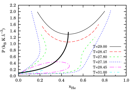
Figure 1: (color online) Schematic pressure-composition phase diagram for six isotherms of the hydrogen-helium mixture at low temperatures and low pressures as drawn in the experimental work by Streett at al. W. B. Streett (1973). The thick continuous black line is the mixture critical line.

For example, the mixture at $T=31~{}\text{K}$ has a lower critical state at $P=0.207~{}k_{B}\text{K}\text{\r{A}}^{-3},x_{\text{He}}=0.214$ and an upper critical state at $P=1.96~{}k_{B}\text{K}\text{\r{A}}^{-3},x_{\text{He}}=0.49$. The set of all critical states constitutes the $x-$line, $T=T_{x}(P)$, such that for $T>T_{x}$ then $x_{\text{He}}^{(I)}=x_{\text{He}}^{(II)}$. The experimental $x-$line of Sneed et al. C. M. Sneed, R. E. Sonntag, and G. J. Van Wylen (1968) is shown in Fig. 2 for the low temperature and low pressure mixture. In the figure we also show the experimental line for the gravitational inversion described in Section III.1.

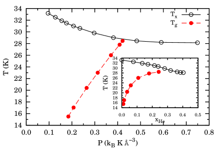
Figure 2: (color online) Reproduction of Fig. 3 of Sneed et al. C. M. Sneed, R. E. Sonntag, and G. J. Van Wylen (1968) for the $x-$line and the $g-$line (see Eq. (13)). The inset shows the two lines in the temperature-composition plane.

For temperatures higher than the hydrogen critical point $T_{\text{H}_{2}}=33.19~{}\text{K}$ ($P_{\text{H}_{2}}=0.094~{}k_{B}\text{K}\text{\r{A}}^{-3}$) there is only an upper critical point W. B. Streett (1973). On the temperature at which $T_{x}(P)$ reaches its minimum there is no unanimous consensus among the various experimental works.

Table 1: Pair-potentials parameters: $\phi_{\text{pair}}$

pair	$\varepsilon^{*}$	$r_{m}^{*}$	$\alpha$	$\beta$	$\gamma$	$C_{6}$	$C_{8}$	$C_{10}$	$D$
He-He	10.8	2.9673	13.208	13.353	0	1.3732	0.42538	0.17810	1.2413
H2-H2	315778	3.41	1.713	10.098	0.41234	1.6955$\times 10^{-4}$	7.2379$\times 10^{-5}$	3.8984$\times 10^{-5}$	1.28
H2-He	14.76	3.375	13.035	13.22	0	1.8310	0	0	0.79802

III Simulation method

We use our QGEMC method, described in Ref. R. Fantoni and S. Moroni (2014), where we monitor the number densities of the two coexisting phases, $\rho^{(i)}=N^{(i)}/V^{(i)}=(N^{(i)}_{\text{He}}+N^{(i)}_{\text{H}_{2}})/V^{(i)}$ with $i=I,II$, the concentrations of He in the two phases, $x_{\text{He}}^{(i)}=N^{(i)}_{\text{He}}/(N^{(i)}_{\text{He}}+N^{(i)}_{\text{H}_{2}})<1$, and the pressure $P$. We shall conventionally order $\rho^{(I)}<\rho^{(II)}$ so that $I$ will be the vapor phase and $II$ the liquid phase, unless $\rho^{(I)}=\rho^{(II)}$, in which case we have a fluid-fluid phase coexistence. In the simulation we fix: $N=N^{(I)}_{\text{He}}+N^{(II)}_{\text{He}}+N^{(I)}_{\text{H}_{2}}+N^{(II)}_{\text{H}_{2}}$ with $N^{(I)}_{\text{H}_{2}}+N^{(II)}_{\text{H}_{2}}=\chi[N^{(I)}_{\text{He}}+N^{(II)}_{\text{He}}]$ and $V=V^{(I)}+V^{(II)}$. Otherwise $N^{(I)}_{\text{He}},N^{(II)}_{\text{He}},N^{(I)}_{\text{H}_{2}},N^{(II)}_{\text{H}_{2}}$ and $V^{(I)},V^{(II)}$ are allowed to fluctuate keeping $V^{(I)}+V^{(II)}$ and $N^{(I)}_{\text{He}}+N^{(II)}_{\text{He}},N^{(I)}_{\text{H}_{2}}+N^{(II)}_{\text{H}_{2}}$ constants. The Gibbs phase rule for a two phase coexistence of a binary mixture assures that one has two independent thermodynamic quantities L. D. Landau and E. M. Lifshitz (1951). So our control parameters will be the absolute temperature $T$ and the global number density $\rho=N/V$ (instead of the pressure as in the experimental case). As usual a finite $N$ sets the size error for our calculation. Whereas $\chi>0$ will regulate the size asymmetry numerical effect so that for

$$N^{(I)}_{\text{He}} = \frac{Nx^{(I)}_{\text{He}}[1-x^{(II)}_{\text{He}}(1+\chi)]}{(1+\chi)(x^{(I)}_{\text{He}}-x^{(II)}_{\text{He}})}>0,$$ (11)

$$N^{(II)}_{\text{He}} = \frac{N}{1+\chi}-N^{(I)}_{\text{He}}>0,$$ (12)

if $x_{\text{He}}^{(II)}<x_{\text{He}}^{(I)}$, we must have $0<x_{\text{He}}^{(II)}<1/(1+\chi)<x_{\text{He}}^{(I)}<1$ and if $x_{\text{He}}^{(I)}<x_{\text{He}}^{(II)}$, then $0<x_{\text{He}}^{(I)}<1/(1+\chi)<x_{\text{He}}^{(II)}<1$. Moreover we must also always have $\rho^{(I)}<\rho<\rho^{(II)}$. The initial condition we chose for our simulations was always as follows: $\rho^{(I)}=\rho^{(II)}=\rho$ and $x_{\text{He}}^{(I)}=x_{\text{He}}^{(II)}=1/(1+\chi)$.

Due to the short-range nature of the effective pair-potentials of Eq. (6) we will approximate, during the simulation, $\phi(r)=0$ for $r>r_{\text{cut}}\gg[r_{m}]_{\text{H}_{2}\text{H}_{2}}$ (this corresponds to the truncated and not shifted choice in Ref. B. Smit (1992)). Where in order to comply with the minimum image convention for the potential energy calculation, we make sure that the conditions $[V^{(i)}]^{1/3}>2r_{\text{cut}}$, for $i=I,II$, are always satisfied during the simulation. This approximation is the only other source of error apart from the size one. The two are related because for instance in the fluid-fluid coexistence, when $V^{(I)}\approx V^{(II)}\approx V/2$ during the simulation, we require $r_{\text{cut}}\approx(N/2\rho)^{1/3}/2\gg[r_{m}]_{\text{H}_{2}\text{H}_{2}}$ for some given $\rho$.

The path integral discretization imaginary time step $\delta\tau=\beta/K$, with $K$ the number of time slices, is chosen so that $\delta\tau^{*}=0.002$, which is considered sufficiently small to justify the use of the primitive approximation of the inter-action D. M. Ceperley (1995). The parameters $\bar{M}$, defined in R. Fantoni and S. Moroni (2014), will be called $\bar{M}_{q}$ for each relevant move $q$ and the parameter $\Delta_{\Omega}$, also defined in R. Fantoni and S. Moroni (2014), is always chosen equal to $0.01$. In order to fulfill detailed balance we must choose $\bar{M}_{2}=\bar{M}_{3}$. In particular we always chose $\bar{M}_{2}=5,\bar{M}_{3}=5,\bar{M}_{4}=5,\bar{M}_{5}=5,\bar{M}_{6}=5$. Regarding the frequency of each move attempts, we always chose $g_{1}=0.001,g_{2}=1,g_{3}=1,g_{4}=1,g_{5}=1,g_{6}=1,g_{7}=0.1$. The parameter $C$ defining the relative weight of the Z and G sectors R. Fantoni and S. Moroni (2014) is adjusted, through short test runs, so as to have a Z sector frequency as close as possible to 50%. We accumulate averages over $10^{5}$ blocks each made of $10^{5}$ attempted moves with quantities measured every $10^{3}$ attempts. Since the volume move is the most computationally expensive one we chose its frequency as the lowest. During the simulation we monitor the acceptance ratios of each move. The various simulations took no more than $\sim 150$ CPU hours on a 3 GHz processor.

III.1 Barotropic phenomenon and gravitational inversion

The condition for the gravitational inversion observed experimentally C. M. Sneed, R. E. Sonntag, and G. J. Van Wylen (1968) is

$$\rho^{(I)}\left(m_{\text{He}}x_{\text{He}}^{(I)}+m_{\text{H}_{2}}x_{\text{H}_{2}}^{(I)}\right)>$$

$$\rho^{(II)}\left(m_{\text{He}}x_{\text{He}}^{(II)}+m_{\text{H}_{2}}x_{\text{H}_{2}}^{(II)}\right),$$ (13)

where $m_{\text{He}}/m_{\text{H}_{2}}=1.98553$. When this condition on the mass density inversion respect to the number density is satisfied, the liquid phase will float on top of the vapor phase. The condition of Eq. (13) can also be rewritten as

$$\rho^{(I)}\left(1+kx_{\text{He}}^{(I)}\right)>\rho^{(II)}\left(1+kx_{\text{He}}^{(II)}\right),$$ (14)

where $k=m_{\text{He}}/m_{\text{H}_{2}}-1=0.98553$. This condition may be satisfied when the concentration of He in the vapor phase is bigger than in the liquid phase, at low temperatures, and the number density of the liquid is close to the one of the vapor, at high pressures. We expect quantum effects to become important in this regime, before solidification which is expected to occur for $T<T_{s}(P)$. The gravitational inversion of Eq. (14) will be satisfied for $T<T_{g}(P)$. The experimental $s$-line $T=T_{s}(P)$ and $g$-line $T=T_{g}(P)$ have been determined in Fig. 3 of Sneed et al. C. M. Sneed, R. E. Sonntag, and G. J. Van Wylen (1968)) in the laboratory.

III.2 Pressure calculation

We will use the virial estimator for the pressure (see Eq. (6.18) of Ref. D. M. Ceperley (1995)). With long-range corrections M. P. Allen and D. J. Tildesley (1987) which can be quite big in the liquid phase. More details on the pressure calculation are given in the supplemental material Sup .

IV Numerical results

Our results are summarized in Table 2 and compared, in Fig. 3, with the experimental data of Refs. W. B. Streett, R. E. Sonntag, and G. J. Van Wylen (1964); C. M. Sneed, R. E. Sonntag, and G. J. Van Wylen (1968); W. B. Streett (1973) (summarized in a Table in the supplemental material Sup ).

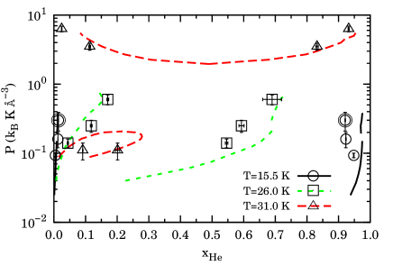
Figure 3: (color online) Comparison between the results of our numerical experiments, points from Table 2, and of the laboratory experiments, lines from Table I in the supplemental material Sup , for the pressure-composition of three isotherms of the hydrogen-helium mixture phase diagram. A logarithmic scale is conveniently used on the ordinates. The double circled points at $T=15.5~{}\text{K}$ denote the case where we observed gravity inversion in the numerical experiment.

In all studied cases we chose $N=128$ and $\delta\tau^{*}=0.002$. We explored the vapor-liquid coexistence (in this work we will denote with “vapor-liquid” coexistence one where $\rho^{(I)}\neq\rho^{(II)}$) at five temperatures, $T=2,5,15.5,26,31$ degrees Kelvin, and the fluid-fluid coexistence (in this work we will denote with “fluid-fluid” coexistence one where $\rho^{(I)}=\rho^{(II)}$) at $T=31~{}\text{K}$. For the first two lower temperatures studied we could not find any experimental data for a comparison. In these two cases when we put a number with trailing dots in the table it means that after the initial equilibration period the measured property did not change anymore during the rest of the simulation.

For the temperature $T=15.5~{}\text{K}$, as it can be readily verified using the relation of Eq. (14), we observe gravitational inversion on the point at $\rho=0.02~{}\text{\r{A}}^{-3}$ when the component with the highest degeneracy temperature is the hydrogen in the liquid phase with $T_{D}\approx 2~{}\text{K}$. Clearly choosing higher pressures quantum statistics will become more and more important for the fluid mixture before reaching the solid state.

For the points at $T=26~{}\text{K}$, $T=31~{}\text{K},\rho=0.006~{}\text{\r{A}}^{-3},\chi=116/12$, and $T=31~{}\text{K},\rho=0.03~{}\text{\r{A}}^{-3},\chi=1$ we observed exchanges of identity between the two phases, during the simulation.

At a temperature $T=31~{}\text{K}$ and a pressure of $P=0.07(2)~{}k_{B}\text{K}\text{\r{A}}^{-3}$ we found a vapor-liquid coexistence, choosing $\chi=116/12$. This point should be subject to greater size error than all other points simulated, and be thus the less reliable, since we only have, in the two boxes, a total of 12 helium atoms. Increasing the pressure to $P=0.21(2)~{}k_{B}\text{K}\text{\r{A}}^{-3}$, in agreement with the experiment, we did not find coexistence and we observed $\rho^{(I)}\approx\rho^{(II)}\approx\rho$ and $x_{\text{He}}^{(I)}\approx x_{\text{He}}^{(II)}\approx 1/(1+\chi)$. Increasing the pressure to $P=3.5(4)~{}k_{B}\text{K}\text{\r{A}}^{-3}$, we did not observe exactly $\rho^{(I)}=\rho^{(II)}$, as measured in the fluid-fluid transition observed in the laboratory W. B. Streett (1973). The same holds true for the point at the same temperature but higher pressure $P=6.3(6)~{}k_{B}\text{K}\text{\r{A}}^{-3}$.

For all measured points except the one at the lower temperature, $T=2~{}\text{K}$ of Table 2, the superfluid fraction E. L. Pollock and D. M. Ceperley (1987) of the two components in either phase was negligibly small. At $T=2~{}\text{K}$ of Table 2, below the helium lambda-temperature, we observed a negligible superfluid fraction of both components in the liquid phase and of the hydrogen in the vapor phase. The helium in the vapor phase was found to have a superfluid fraction of $0.012(3)$, indicating a tendency to supefluidity.

When we do not observe exchanges of identity between the two phases, during the simulation, we are able to find accurate average values for the various measured quantities. Otherwise a histogram analysis of the data is necessary with a non-linear fit using the superpositions of two shifted Gaussians. For example in Fig. 4 we show the procedure used to extract the helium concentrations of the two coexisting phases for the case $T=26~{}\text{K},\rho=0.01~{}\text{\r{A}}^{-3},\chi=90/38$.

Figure 4: Fit of the histogram for the block averages of both $x_{He}^{(I)}$ and $x_{He}^{(II)}$ with the sum of two gaussians with six parameters. This is case $T=26~{}\text{K},\rho=0.01~{}\text{\r{A}}^{-3},\chi=90/38$, where we had box identity excanges.

The measured property which is less accurate is the pressure due to the size error and the long-range correction dependent on the $r_{\text{cut}}$ choice. This problem could be overcome by using instead of the $N,V,T$ version of the Gibbs ensemble algorithm its $N,P,T$ one D. Frenkel and B. Smit (1996).

Table 2: Numerical isothermal pressure-composition at coexistence. We always used $N=128$ and $\delta\tau^{*}=0.002$.

$T~{}(\text{K})$	$\rho~{}(\text{\r{A}}^{-3})$	$\chi$	$P~{}(k_{B}\text{K}\text{\r{A}}^{-3})$	$x_{\text{He}}^{(II)}$	$x_{\text{He}}^{(I)}$	$\rho^{(II)}~{}(\text{\r{A}}^{-3})$	$\rho^{(I)}~{}(\text{\r{A}}^{-3})$
2.0	0.015	1	$-$0.08(7)	0.214$\ldots$	0.639$\ldots$	0.02456(1)	0.012605(2)
5.0	0.010	1	0.014(2)	0.1787(1)	1.000$\ldots$	0.025910(6)	0.005113(1)
15.5	0.010	1	0.093(7)	0.00457(9)	0.948(1)	0.02410(1)	0.006544(5)
15.5	0.015	1	0.16(4)	0.0125(3)	0.923(1)	0.02304(2)	0.011525(7)
15.5	0.020	1	0.30(9)	0.0142(4)	0.921(1)	0.02373(2)	0.017619(5)
26.0	0.010	90/38	0.14(2)	0.044(2)	0.546(4)	0.01890(5)	0.00669(1)
26.0	0.015	90/38	0.25(5)	0.118(3)	0.593(8)	0.01888(7)	0.01105(5)
26.0	0.020	90/38	0.6(1)	0.170(3)	0.69(3)	0.02115(2)	0.01759(8)
31.0	0.006	116/12	0.11(3)	0.091(1)	0.201(7)	0.014(2)	0.00564(6)
31.0	0.008	1	0.21(2)	0.5025(6)	0.511(1)	0.008016(7)	0.00795(1)
31.0	0.030	1	3.5(4)	0.832(4)	0.113(3)	0.03198(4)	0.02805(1)
31.0	0.035	1	6.3(6)	0.932(2)	0.0243(9)	0.03955(5)	0.03111(1)

IV.1 Finite size effects

We studied the finite size effects at $T=31~{}\text{K},\rho=0.03~{}\text{\r{A}}^{-3},\chi=1$. In Table 3 we show the results for the isothermal pressure-composition coexistence at $N=64,128,$ and $256$. As the number of particles increases we observe a decrease in the ratio of number of exchanges of identity between the two phases and total number of particles: For $N=64$ the exchanges occurred many times, for $N=128$ only once, and for $N=256$ never. For the case $N=64$ we found the peak of the first gaussian for the hystogram of $x_{\text{He}}$ with a negative value. The simulation with $N=64$ took $1.0\times 10^{5}$s, the one with $N=128$ took $1.6\times 10^{5}$s, and the one with $N=256$ took $4.0\times 10^{6}$s. From the comparison we see how there is not much difference between $N=128$ and $N=256$. Apart from the smaller statistical errors in the latter case, the concentrations slightly differ in the two cases.

Table 3: Numerical isothermal pressure-composition coexistence at $T=31~{}\text{K},\rho=0.03~{}\text{\r{A}}^{-3},\chi=1$ as a function of the number of particles $N$. We always used $\delta\tau^{*}=0.002$.

$N$	$r_{\text{cut}}(\text{\r{A}})$	$P~{}(k_{B}\text{K}\text{\r{A}}^{-3})$	$x_{\text{He}}^{(II)}$	$x_{\text{He}}^{(I)}$	$\rho^{(II)}~{}(\text{\r{A}}^{-3})$	$\rho^{(I)}~{}(\text{\r{A}}^{-3})$
64	5	2.4(8)	0.83(3)	-	0.03144(7)	0.02782(3)
128	6	3.5(4)	0.832(4)	0.113(3)	0.03198(4)	0.02805(1)
256	8	3.4(2)	0.840(3)	0.098(3)	0.03180(3)	0.028170(9)

IV.2 Importance of the particle exchanges and of the quantum effects

Setting to zero the frequency of the swap move attempts our algorithm reduces to a path integral calculation for distinguishable particles obeying to the Boltzmann statistics. On the other hand, choosing $K=2$ (with $\bar{M}_{q}=1$ for all $q$) and $\lambda^{*}_{\text{H}_{2}}=\lambda^{*}_{\text{He}}\to 0$ it reduces to the classical Gibbs Ensemble Monte Carlo (GEMC) algorithm of Panagiotopoulos A. Z. Panagiotopoulos (1987).

For the state point $T=15.5~{}\text{K}$ and $\rho=0.02~{}\text{\r{A}}^{-3}$ with $N=128$, we performed two simulations for each of the two cases suggested above to estimate the importance of particles exchanges which underlies the Bose-Einstein statistics and of quantum effects, respectively. To reach the GEMC limit from our QGEMC algorithm we chose, in particular, $\lambda^{*}_{\text{H}_{2}}=\lambda^{*}_{\text{He}}=10^{-3}$. The results are shown in Table 4. The acceptance ratio for the swap move was around $0.5$ in the full quantum case and imposed zero in the other two simulations.

As we can see from the table, for this state point, there is a very small difference between the path integral simulation with the full Bose-Einstein statistics and the one with the Boltzmann statistics. In particular, only the densities of the vapor phase are different in the two cases. In both these simulations we observe the gravitational inversion. We expect that increasing the pressure and thereby the density or reducing the temperature the particles exchanges will become increasingly important.

On the other hand, there is a large difference between these two simulations and the classical GEMC one. In particular, the gravitational inversion is not observed in the classical limit simulation, even if after a short equilibration time the simulation converged towards the condition $x_{\text{He}}^{(I)}=1$, i.e. all helium atoms, the heaviest species in the mixture, were found in the less dense phase.

Table 4: Numerical isothermal pressure-composition coexistence at $T=15.5~{}\text{K},\rho=0.02~{}\text{\r{A}}^{-3},\chi=1$ in a simulation with the full QGEMC algorithm with the Bose-Einstein statistics ($\delta\tau^{*}=0.002$), with the QGEMC algorithm with Boltzmann statistics ($\delta\tau^{*}=0.002$), and with the GEMC limit (see main text) of the QGEMC algorithm. We always used $N=128$.

Statistics	$P~{}(k_{B}\text{K}\text{\r{A}}^{-3})$	$x_{\text{He}}^{(II)}$	$x_{\text{He}}^{(I)}$	$\rho^{(II)}~{}(\text{\r{A}}^{-3})$	$\rho^{(I)}~{}(\text{\r{A}}^{-3})$
QGEMC: Bose-Einstein	0.30(9)	0.0142(4)	0.921(1)	0.02373(2)	0.017619(5)
QGEMC: Boltzmann	0.30(9)	0.0143(4)	0.919(1)	0.02373(2)	0.017638(5)
GEMC: classical limit	0.13(4)	0.000$\ldots$	1.000$\ldots$	0.035953(5)	0.0138552(7)

V Conclusions

In conclusion, we performed path integral Monte Carlo simulations, using our newly developed QGEMC method, for the two phase coexistence of the hydrogen-helium mixture away from freezing. This asymmetric mixture displays at low temperature, a big concentration asymmetry in the two coexisting phases, whereas the densities of the two phases tend to become equal at high pressure. This is responsible for a gravitational inversion, where the liquid, the more dense phase, with an abundance of hydrogen, floats above the vapor, the less dense phase, with an abundance of helium. In this coexistence region of the temperature-pressure diagram, quantum statistics is expected to play an important role and in our simulations we are able to observe such gravitational inversion. Our numerical experiments are also in good quantitative agreement with the experimental results of C. M. Sneed, W. B. Streett, R. E. Sonntag, and G. J. Van Wylen in the late 1960’s and early 1970’s. The difference between our results on the helium concentration in the two phases and the experimental ones is in all cases less than 15% in the high helium concntration phase and than 5% in the low helium concentration phase, relative to the experiment.

These results for the hydrogen-helium mixture can be of interest for the study of cold exoplanets with an atmosphere made predominantly by such a fluid mixture and with the right temperature and pressure conditions for there to be coexistence. In such cases it could be possible to observe the gravitational inversion phenomenon and consequent changes in the planet moment of inertia, depending on the atmospherical and climatic conditions.

At extremely low temperature and pressure we find that the first component to show superfluidity is the helium in the vapor phase.

Our QGEMC method R. Fantoni and S. Moroni (2014) is extremely simple to use, reduces to the Gibbs ensemble method of Panagiotopoulos A. Z. Panagiotopoulos (1987) in the classical regime, and gives an exact numerical solution of the statistical physics phase coexistence problem for boson fluids.

An open problem, currently under exam, is the influence of the finite-size effects on the determination of the binodal curves close to the lower strongly asymmetric critical points, as for example in our case $T=31~{}\text{K},\rho=0.006~{}\text{\r{A}}^{-3},\chi=116/12$. This requires additional simulations at an higher and lower number of particles.

References

- W. B. Streett, R. E. Sonntag, and G. J. Van Wylen (1964) W. B. Streett, R. E. Sonntag, and G. J. Van Wylen, J. Chem. Phys. 40, 1390 (1964).
- R. E. Sonntag, G. J. Van Wylen, and R. W. Crain, Jr. (1964) R. E. Sonntag, G. J. Van Wylen, and R. W. Crain, Jr., J. Chem. Phys. 41, 2399 (1964).
- C. M. Sneed, R. E. Sonntag, and G. J. Van Wylen (1968) C. M. Sneed, R. E. Sonntag, and G. J. Van Wylen, J. Chem. Phys. 49, 2410 (1968).
- W. B. Streett (1973) W. B. Streett, The Astrophysical Journal 186, 1107 (1973).
- L. C. Van Den Bergh, J. A. Schouten, and N. J. Trappeniers (1987) L. C. Van Den Bergh, J. A. Schouten, and N. J. Trappeniers, Physica A 141, 524 (1987).
- B. Militzer (2005) B. Militzer, Journal of Low Temperature Physics 139, 739 (2005).
- M. A. Morales, E. Schwegler, D. Ceperley, C. Pierleoni,S. Hamel, and K. Caspersen (2009) M. A. Morales, E. Schwegler, D. Ceperley, C. Pierleoni,S. Hamel, and K. Caspersen, Proc. Natl. Acad. Sci. USA 106, 1324 (2009).
- W. Lorenzen, B. Holst, and R. Redmer (2009) W. Lorenzen, B. Holst, and R. Redmer, Phys. Rev. Lett. 102, 115701 (2009).
- W. Lorenzen, B. Holst, and R. Redmer (2011) W. Lorenzen, B. Holst, and R. Redmer, Phys. Rev. B 84, 235109 (2011).
- J. M. McMahon, M. A. Morales, C. Pierleoni, and D. M. Ceperley (2012) J. M. McMahon, M. A. Morales, C. Pierleoni, and D. M. Ceperley, Rev. Mod. Phys. 84, 1607 (2012).
- M. A. Morales, S Hamel, K. Caspersen, and E. Schwegler (2013) M. A. Morales, S Hamel, K. Caspersen, and E. Schwegler, Phys. Rev. B 87, 174105 (2013).
- F. Soubiran, S. Mazevet, C. Winisdoerffer, and G. Chabrier (2013) F. Soubiran, S. Mazevet, C. Winisdoerffer, and G. Chabrier, Phys. Rev. B 87, 165114 (2013).
- R. Fantoni (2014) R. Fantoni, Phys. Rev. E 90, 020102(R) (2014).
- R. Fantoni and S. Moroni (2014) R. Fantoni and S. Moroni, J. Chem. Phys. 141, 114110 (2014).
- Y. S. Wei and R. J. Sadus (1996) Y. S. Wei and R. J. Sadus, Fluid Phase Equilibria 122, 1 (1996).
- D. M. Ceperley (1995) D. M. Ceperley, Rev. Mod. Phys. 67, 279 (1995).
- R. A. Aziz, V. P. S. Nain, J. S. Carley, W. L. Taylor, and G. T. McConville (1979) R. A. Aziz, V. P. S. Nain, J. S. Carley, W. L. Taylor, and G. T. McConville, J. Chem. Phys. 70, 4330 (1979).
- I. F. Silvera and V. V. Goldman (1978) I. F. Silvera and V. V. Goldman, J. Chem. Phys. 69, 4209 (1978).
- E. A. Mason and W. E. Rice (1954) E. A. Mason and W. E. Rice, J. Chem. Phys. 22, 522 (1954).
- C. S. Roberts (1963) C. S. Roberts, Phys. Rev. 131, 203 (1963).
- (21) See Supplemental Material at .
- L. D. Landau and E. M. Lifshitz (1951) L. D. Landau and E. M. Lifshitz, Statistical Physics, part 1, 3rd ed., Course of Theoretical Physics (Butterworth Heinemann, Oxford, 1951) §86.
- B. Smit (1992) B. Smit, J. Chem. Phys. 96, 8639 (1992).
- M. P. Allen and D. J. Tildesley (1987) M. P. Allen and D. J. Tildesley, Computer Simulation of Liquids (Clarendon Press, Oxford, 1987) section 2.8.
- E. L. Pollock and D. M. Ceperley (1987) E. L. Pollock and D. M. Ceperley, Phys. Rev. B 36, 8343 (1987).
- D. Frenkel and B. Smit (1996) D. Frenkel and B. Smit, Understanding Molecular Simulation (Academic Press, San Diego, 1996) chapter 8.
- A. Z. Panagiotopoulos (1987) A. Z. Panagiotopoulos, Mol. Phys. 61, 813 (1987).