Berry phase and anomalous velocity of Weyl fermions and Maxwell photons

Abstract

We consider two systems of wave equations whose wave-packet solutions have trajectories that are altered by the “anomalous velocity” effect of a Berry curvature. The first is the matrix Weyl equation describing cyclotron motion of a charged massless fermion. The second is Maxwell equations for the whispering-gallery modes of light in a cylindrical waveguide. In the case of the massless fermion, the anomalous velocity is obscured by the contribution from the magnetic moment. In the whispering gallery modes the anomalous velocity causes the circumferential light ray to creep up the cylinder at the rate of one wavelength per orbit, and can be identified as a continuous version of the Imbert-Federov effect.

I Introduction

In many quantum systems the motion of a wave-packet is governed by semiclassical equations of the form [1, 2, 3, 4]

$$\dot{\bf k} = -{\partial{\mathcal{H}}\over\partial{\bf x}}+e(\dot{\bf x}\times{\bf B}),$$ (1)

$$\dot{\bf x} = {\partial{\mathcal{H}}\over\partial{\bf k}}+\dot{\bf k}\times{\mbox{\boldmath$\Omega$}}.$$ (2)

In the absence of the last term in the second equation these would just be Hamilton’s equations for a particle with hamiltonian ${\mathcal{H}}({\bf x},{\bf k})=\varepsilon({\bf k})+V({\bf x})$ moving in a magnetic field. The additional $\dot{\bf k}\times{\mbox{\boldmath$\Omega$}}$ term in (2) is the anomalous velocity correction to the naïve group velocity $\partial\varepsilon/\partial{\bf k}$.

The vector ${\bf\Omega}$ is a function of the kinetic momentum ${\bf k}$ only, and is a Berry curvature which has different origins in different systems. For a Bloch electron in an energy band in a solid the curvature accounts for the effects of all other bands. In particle-physics applications the curvature arises from the intrinsic angular momentum of the particle. In all cases it affects the velocity because different momentum components of a localized wave-packet accumulate different geometric phases when both ${\bf k}$ is changing and the Berry curvature is non-zero [5]. These ${\bf k}$-dependent geometric phases are just as significant in determining the wave-packet position as the ${\bf k}$-dependent dynamical phases arising from the dispersion equation $\omega=\varepsilon({\bf k})$.

A particularly simple example occurs in in the dynamics of massless relativistic fermions and in Weyl semimetals where bands touch at a point. In both systems the wavepackets are solutions of a Weyl “half-Dirac” equation and the Berry curvature arises because the spin (or pseudo-spin) vector is locked to the direction of the momentum ${\bf k}$. The forced precession of a spin-$S$ vector is the paradigm in the original Berry-phase paper [6] and the corresponding curvature is simply

$${\mbox{\boldmath$\Omega$}}({\bf k})=S{{\bf k}\over|{\bf k}|^{3}}.$$ (3)

Even this basic example gives rise to much physics — the axial and gauge anomalies [7, 8, 9] and the chiral magnetic and vortical effect [10, 11, 12].

The semiclassical analyses that reveal the anomalous velcity in (2) are quite intricate as they have to go beyond the leading WKB ray tracing equation. It is the aim of this paper to consider two simple systems in which the predicted anomalous velocity effect can be sought directly in the stationary eigenfunctions of underlying wave equation. In both cases the curvature is given by (3). The first (in section II) is the circular motion of a massless charged spin-1/2 particle in a magnetic field. The second (in section III) is the circular motion of a spin-1 photon in an optical fibre waveguide. In the first case the presence of the anomalous velocity is obscured by the coupling of the magnetic field to the particle’s magnetic moment. The second unambiguously displays the expected anomalous velocity drift.

II Cyclotron orbits

We start by considering the cyclotron motion of a massless Weyl fermion with positive charge $e$ in a magnetic field ${\bf B}=-B\hat{\bf z}$. The field is derived from a vector potential ${\bf A}=B(y,-x)/2$ and its downward direction has been chosen so that the particle orbits in an anti-clockwise direction about the $z$ axis.

The Weyl Hamiltonian for a right-handed spin-1/2 particle is

$$H=-i{\mbox{\boldmath$\sigma$}}\cdot(\nabla-ie{\bf A}),$$ (4)

where ${\mbox{\boldmath$\sigma$}}=(\sigma_{1},\sigma_{2},\sigma_{3})$ denotes the Pauli matrices. We are using natural units in which $\hbar=c=1$, although we will occasionally insert these symbols when it helps to illuminate the discussion.

Acting on functions proportional to $e^{ik_{z}z}$ we have

$$H^{2}={\mathbb{I}}\left(-\nabla^{2}+{e^{2}B^{2}\over 4}r^{2}+eBL_{3}+k_{z}^{2}\right)+eB\sigma_{3},$$ (5)

where $L_{z}=-i(x\partial_{y}-y\partial x)=-i\partial_{\phi}$ is the canonical (as opposed to kinetic) angular momentum and ${\mathbb{I}}$ denotes the 2-by-2 identity matrix. The eigenvalues of the scalar Shrödinger operator in parenthesis in (5) are

$$E^{2}_{n,l,k_{z}}=eB\left\{2n+|l|+l+1\right\}+k_{z}^{2},$$ (6)

and the corresponding eigenfunctions are

$$\varphi_{n,l,k_{z}}(r,\phi)=\left({eB\over 2}\right)^{(|l|+1)/2}\sqrt{{n!\over(n+|l|)!}}r^{|l|}\exp\left(-{eBr^{2}\over 4}\right)L^{|l|}_{n}\left({eBr^{2}\over 2}\right)e^{il\phi}e^{ik_{z}z}.$$ (7)

Both $n$ and $l$ are integers and $L^{|l|}_{n}$ is the associated Laguerre polynomial. When $n=0$, $k_{z}=0$, and $l>0$, the wavefunction $\varphi_{0,l,0}(r,\phi)$ corresponds to a particle describing a circular cyclotron orbit with the origin as its centre and radius

$$R_{l}=\sqrt{{2l\over eB}}.$$ (8)

If we decrease $l$ while staying in the same Landau level (i.e.  by increasing $n$ so as to keep $E^{2}_{n,l}$ fixed) the classical circular orbit keeps the same radius but its centre moves away from the origin and is smeared-out in $\theta$ over the full $2\pi$. When $l=0$ the circle passes through the origin. For $l$ negative, the energy no longer depends on $l$ and the Landau level keeps $n$ fixed while $l$ continues to decrease. The classical orbit still has the original radius, but no longer encloses the origin. In particular the case $n=k_{z}=0$ and $l<0$ corresponds particles in the lowest Landau level but with different orbit centres.

By applying the projection operator $P=(E+H)/2E$ to the Schrödinger eigenfunction we find that the cyclotron-motion eigenfunctions of the Weyl hamiltonian $H$ with $n=0$, $l>0$, and longitudinal momentum $k_{z}$ are

$$\psi_{0,l,k_{z}}(r,\theta,z)=e^{ikz}e^{il\phi}\left[\begin{matrix}(E_{l,k_{z}}+k_{z})r^{-1}e^{-i\phi}\cr ieB\end{matrix}\right]r^{l}\exp\left(-{eBr^{2}\over 4}\right).$$ (9)

These states have energy $E_{l,k_{z}}=\sqrt{2leB+k_{z}^{2}}$ and the orbit radius is still

$$R_{l}=\sqrt{{2l\over eB}}.$$ (10)

At $k_{z}=0$, the angular velocity of a wave-packet is

$$\dot{\phi}=\left.{\partial E_{l,k_{z}}\over\partial l}\right|_{k_{z}=0}=\sqrt{{eB\over 2l}}$$ (11)

ensuring that $v_{\phi}=R_{l}\dot{\phi}=c=1$.

There is a special case where $l=n=0$ and

$$\psi_{0,0,k_{z}}=e^{ik_{z}z}\left(\begin{matrix}0\cr 1\end{matrix}\right)\exp\left(-{eB|z|^{2}\over 4}\right)$$ (12)

with $E=-k_{z}$. This mode only exists as a positive energy mode for $k_{z}<0$. It is this unbalanced mode, with a density of $eB/2\pi$ per unit area in the $x$, $y$ plane that is the source of the chiral-magnetic-effect current

$${\bf J}_{\rm CME}={e^{2}{\bf B}\over 2\pi}\int_{0}^{\mu}{dk_{z}\over 2\pi}={e^{2}\over 4\pi^{2}}{\bf B}\mu,$$ (13)

of a gas of zero-temperature Weyl fermions with chemical potential $\mu$ [10, 11].

Consider the $l>0$, $k_{z}=0$ orbits. Even though these orbits possess no component of momentum in the $z$ direction, plugging the time dependence of the classical orbital momentum ${\bf k}$ into the anomalous-velocity formula (2) suggests that they should creep down the $z$ axis. To compute the predicted creep-rate we observe that a particle of helicity $S$ whose spin direction is forced to describe a circle of co-latitude $\theta$ on a sphere with polar co-ordinates $\theta$, $\phi$ accumulates Berry phase at the rate [6]

$$\dot{\gamma}_{\rm Berry}=-S(1-\cos\theta)\dot{\phi}.$$ (14)

For $S=+1/2$, and using our expression for $\dot{\phi}$, this becomes

$$\dot{\gamma}_{\rm Berry}={1\over 2}(\cos\theta-1)\dot{\phi}={1\over 2}(\cos\theta-1)\sqrt{{eB\over 2l}}.$$ (15)

where

$$\cos\theta={k_{z}\over\sqrt{2leB+k_{z}^{2}}}\sim{k_{z}\over\sqrt{2leB}}.$$ (16)

In an energy eigenstate this accumulating geometric phase should be indistinguishable from the accumulating $-Et$ dynamical phase. In other words $\dot{\gamma}_{\rm Berry}$ should appear as a contribution to the energy of

$$E_{\rm Berry} = {\rm const}.-{1\over 2}{k_{z}\over\sqrt{2leB+k_{z}^{2}}}\sqrt{{eB\over 2l}}$$ (17)

$$\sim {\rm const}.-{1\over 2}{k_{z}\over 2l}.$$

This energy adds

$$\dot{z}={\partial E_{\rm Berry}\over\partial k_{z}}=-{1\over 2}{1\over 2l}$$ (18)

to the group velocity over above that expected from the $E=c|{\bf k}|$ energy-momentum relation. The velocity (18) corresponds to drift rate of one-half of a de Broglie wavelength $\lambda_{\rm Broglie}$ per orbit — the de Broglie wavelength being here defined as the wavelength associated with the kinetic momentum ${\bf k}$ so that $E={2\pi\hbar c}/{\lambda_{\rm Broglie}}$.

Unfortunately, except for the special case $l=0$, there is no sign of any contribution to the energy linear in $k_{z}$ in the exact solution of the eigenvalue problem! Instead we have

$$E=\sqrt{2leB+k_{z}^{2}}=\sqrt{2leB}+{1\over 2}k_{z}^{2}/\sqrt{2leB}+\cdots.$$ (19)

The reason for the absence is that there is another linear-in-$k_{z}$ contribution to the energy coming from the Weyl particle’s magnetic moment [12].

One might question whether a massless particle can have a magnetic moment as no time ever passes on a null-vector world-line. Nonetheless, in the laboratory frame, a particle obeying the Weyl equation possesses an energy-dependent effective moment of

$${\mbox{\boldmath$\mu$}}_{\rm Weyl}=\pm{e\hat{\bf k}\over 2E}.\quad\hbox{($\pm$ for positive/negative helicity)}.$$

This moment is precisely what is required for the Larmor precession frequency

$$\Omega_{\rm Larmor}=-B\left|{\mbox{\boldmath$\mu$}\over\bf S}\right|$$

to coincide with the orbital frequency and so ensure that the spin remains aligned with the momentum. The appendix contains a derivation of ${\mbox{\boldmath$\mu$}}_{\rm Weyl}$ from the Weyl equation and explains how the Dirac gyromagnetic ratio $g=2$ continues to to be valid even for massless particles. For a positive-helicity particle the interaction of this moment with the magnetic field provides an energy shift of

$$\delta E_{\rm magnetic}=-{\mbox{\boldmath$\mu$}}_{\rm Weyl}\cdot{\bf B}=-{e{\bf B}\cdot{\hat{\bf k}}\over 2E}={eB\cos\theta\over 2\sqrt{2leB}}=+{1\over 2}{k_{z}\over 2l}.$$

that precisely cancels the Berry phase contribution. This cancellation does not apply to all eigenstates and does not affect the total chiral magnetic effect, but as explained in [12] it does complicate its simple semiclassical derivation in [7].

III Photons in whispering-gallery modes

We were thwarted in our attempt to observe an anomalous drift velocity in an exact solution of the Weyl equation because the accumulating geometric Berry phase was obscured by a dynamical phase arising from the particle’s magnetic moment. We therefore seek the effect in the motion of a moment-free massless spinning particle. An obvious candidate is the spin-1 photon. To make it clear that a photon should obey similar semiclassical equations to a massless fermion it helps to rewrite Maxwell’s equations in a form that affords a direct comparison with the Weyl equation. The idea for a such a rewriting is apparently due to Riemann. The complete set of Maxwell’s equations equations were first published in 1865 and Riemann died in 1866. The rewriting is nonetheless ascribed to him by Heinrich Weber in his edition of Riemann’s lectures published in 1901 [13]. The idea was independently discovered by Silberstein [14] in 1907, and has been recently extensively championed by the Białynicki-Birula’s [15]. The Riemann-Silberstein equations make use the complex-valued fields

$${\mbox{\boldmath$\Psi$}}^{\pm} = {\bf E}\pm ic{\bf B}$$ (20)

$$= {\bf E}\pm iZ{\bf H},$$

where

$$Z=\sqrt{{\mu\over\epsilon}}$$ (21)

is the wave impedance. Provided that $Z$ does not vary with position or time, we can combine the two Maxwell “curl” equations as

$$i\partial_{t}\Psi^{\pm}_{i}=\pm c_{\rm local}\,\epsilon_{ijk}\partial_{j}\Psi^{\pm}_{k}.$$ (22)

Here $c_{\rm local}\equiv 1/\sqrt{\mu\epsilon}$ may vary with position. At non-zero frequency, the two Maxwell “divergence” equations follow from curl equations and do not need to be separately imposed. Once we define the spin-1 generator ${\mbox{\boldmath$\Sigma$}}_{i}$ to be the matrix with entries $-i\epsilon_{ijk}$, eq. (22) becomes a pair of Weyl equations

$$i\hbar\partial_{t}{\mbox{\boldmath$\Psi$}}^{\pm}=\pm c_{\rm local}\,({\mbox{\boldmath$\Sigma$}}\cdot\hat{\bf p}){\mbox{\boldmath$\Psi$}}^{\pm},$$ (23)

one for the left-helicity chiral field and one for the right-helicity field. to make the analogy with the Dirac-Weyl equation as close as possible, we have inserted an $\hbar$ on both sides of (22) so that we can exhibit the equation in terms of the quantum mechanical momentum operator $\hat{\bf p}=-i\hbar\nabla$. We conclude that as the direction of the wave-momentum vector precesses, the photon spin is forced to follow it. The photon wavefunction will then acquire a geometric Berry phase that is twice as a large as that of the Weyl fermion, and this phase must have a similarly-proportioned effect on the semi-classical particle trajectory.

The only significant difference between the spin-$1/2$ Weyl equation and Maxwell equations is that the Maxwell “wave-function” obeys a Majorana condition

$$({\mbox{\boldmath$\Psi$}}^{+})^{*}={\mbox{\boldmath$\Psi$}}^{-}$$ (24)

that indicates that the photon is its own antiparticle.

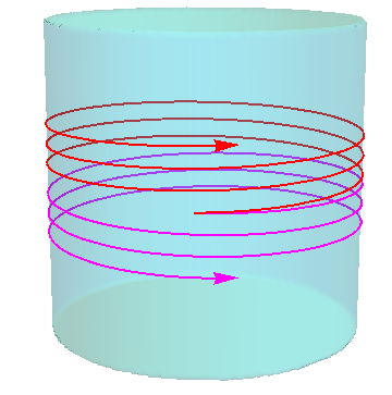
Figure 1: The separation of the positive helicity circumferential ray (magenta) from the negative helicity ray (red) in a cylindrical dielectric waveguide. Wavepackets drift up and down the fiber at the rate of one wavelength per turn.

To obtain an optical analogue of cyclotron motion, we consider the whispering-gallery modes of light in a step-index optical fibre. In whispering-gallery modes a light beam orbits the fibre circumferentially rather than propagating along its length. We may think of the orbit as a closely spaced sequence of total internal reflections off the step discontinuity in the refractive index. (See figure 1). A separation of the orbits of left and right circularly polarized beams was predicted from the anomalous velocity equations in [16] and experimentally verified in [17]. In this section we seek to derive the separation directly from the Maxwell-equation eigenmodes.

Recall that the refractive index $n$ is obtained from the material parameters as $n/c=\sqrt{\epsilon\mu}$ and, in natural units where $c=1$, the local speed of light is $1/n$. We take the axis of the fibre as the $z$ axis and its core to have refractive index $n=n_{1}$ for $r<R$. The cladding will have index $n=n_{2}$ for $r>R$. All fields will have a tacit factor of $e^{ik_{z}z-i\omega t}$ so our differential operators act only on functions of the transverse co-ordinates $x$, $y$. We define parameters $\gamma$ by

$$\gamma^{2}=\pm(\epsilon\mu\omega^{2}-k_{z}^{2})$$ (25)

where the sign is chosen so that $\gamma$ is real.

The transverse field components ${\bf E}_{\perp}$ and ${\bf H}_{\perp}$ are expressed in terms of the longitudinal components $E_{z}$ and $H_{z}$ by

$${\bf E}_{\perp} = {i\over\gamma^{2}}\left\{k_{z}\nabla_{\perp}E_{z}-\omega\mu\,{\bf e}_{z}\times\nabla_{\perp}H_{z}\right\},$$

$${\bf H}_{\perp} = {i\over\gamma^{2}}\left\{k_{z}\nabla_{\perp}H_{z}+\omega\epsilon\,{\bf e}_{z}\times\nabla_{\perp}E_{z}\right\},$$ (26)

where, for our step fibre (no gradients of $\epsilon$ or $\mu$ away from the discontinuity)

$$-\nabla_{\perp}^{2}H_{z}+(k_{z}^{2}-\epsilon\mu\omega^{2})H_{z} = 0,$$

$$-\nabla_{\perp}^{2}E_{z}+(k_{z}^{2}-\epsilon\mu\omega^{2})E_{z} = 0.$$ (27)

To be guided we need $k_{z}^{2}-\epsilon\mu\omega^{2}$ to be negative in the core, and positive in the cladding. The solutions to (27) are then

$$E_{z}=\begin{cases}A{\rm J}_{l}(\gamma_{1}r)e^{il\theta},&r<R,\\ B{\rm K}_{l}(\gamma_{2}r)e^{il\theta},&r>R,\end{cases}$$ (28)

$$H_{z}=\begin{cases}C{\rm J}_{l}(\gamma_{i}r)e^{il\theta},&r<R,\\ D{\rm K}_{l}(\gamma_{2}r)e^{il\theta},&r>R.\end{cases}$$ (29)

Here ${\rm J}_{l}$ and ${\rm K}_{l}$ are the Bessel function and modified Bessel function respectively.

Below the fibre cutoff frequency the quantity $\gamma^{2}=\epsilon\mu\omega^{2}-k_{z}^{2}$ is always positive. Light is no longer completely confined, so the eigen-frequencies have a negative imaginary that implies an exponential decay in time. The corresponding eigenfunctions must have outgoing waves at infinity, and so will be of the form

$$E_{z}=\begin{cases}A{\rm J}_{l}(\gamma_{i}r)e^{il\theta},&r<R,\\ B{\rm H}^{(1)}_{l}(\gamma_{2}r)e^{il\theta},&r>R,\end{cases}$$ (30)

$$H_{z}=\begin{cases}C{\rm J}_{l}(\gamma_{i}r)e^{il\theta},&r<R,\\ D{\rm H}^{(1)}_{l}(\gamma_{2}r)e^{il\theta}.&r>R,\end{cases}$$ (31)

Here ${\rm H}^{(1)}_{l}$ is a Hankel function of the first kind.

Whispering-gallery modes have small $k_{z}$ and large azimuthal quantum number $l$. These modes are always below the fibre cutoff, and so $\gamma^{2}$ does not change sign at $r=R$. If we consider the waves near the point $(x,y,z)=(R,0,0)$ then we have

$$E_{x} = {i\over\gamma^{2}}\left(k_{z}{\partial E_{z}\over\partial r}-{\omega\mu\over r}{\partial H_{z}\over\partial\theta}\right)$$

$$E_{y} = {i\over\gamma^{2}}\left({k_{z}\over r}{\partial E_{z}\over\partial\theta}+{\omega\mu}{\partial H_{z}\over\partial r}\right)$$

$$H_{x} = {i\over\gamma^{2}}\left(k_{z}{\partial H_{z}\over\partial r}+{\omega\epsilon\over r}{\partial E_{z}\over\partial\theta}\right)$$

$$H_{y} = {i\over\gamma^{2}}\left({k_{z}\over r}{\partial H_{z}\over\partial\theta}-{\omega\epsilon}{\partial E_{z}\over\partial r}\right)$$ (32)

On substituting the functional form of the solutions for $r<R$ these become

$$E_{x} = {i\over\gamma_{1}^{2}}\left(k_{z}\gamma_{1}{\rm J^{\prime}}_{l}(\gamma_{1}r)A-{il\omega\mu\over r}{\rm J}_{l}(\gamma_{1}r)C\right)$$

$$E_{y} = {i\over\gamma_{1}^{2}}\left({ik_{z}l\over r}{\rm J}_{l}(\gamma_{1}r)A+{\omega\mu}\gamma_{1}{\rm J^{\prime}}_{l}(\gamma_{1}r)C\right)$$

$$H_{x} = {i\over\gamma_{1}^{2}}\left(k_{z}\gamma_{1}J^{\prime}(\gamma_{1}r)C+{il\omega\epsilon\over r}{\rm J}_{l}(\gamma_{1}r)A\right)$$

$$H_{y} = {i\over\gamma_{1}^{2}}\left({ik_{z}l\over r}{\rm J}_{l}(\gamma_{1}r)C-{\omega\epsilon\gamma_{1}}{\rm J^{\prime}}_{l}(\gamma_{1}r)A\right),$$ (33)

and for $r>R$

$$E_{x} = {i\over\gamma_{2}^{2}}\left(k_{z}\gamma_{2}{\rm H^{\prime}}^{(1)}_{l}(\gamma_{2}r)B-{il\omega\mu_{2}\over r}{\rm H}^{(1)}_{l}(\gamma_{2}r)D\right)$$

$$E_{y} = {i\over\gamma_{2}^{2}}\left({ik_{z}l\over r}{\rm H}^{(1)}_{l}(\gamma_{2}r)B+{\omega\mu_{2}}\gamma_{2}{\rm H^{\prime}}^{(1)}_{l}(\gamma_{2}r)D\right)$$

$$H_{x} = {i\over\gamma_{2}^{2}}\left(k_{z}\gamma_{2}{\rm H^{\prime}}^{(1)}_{l}(\gamma_{2}r)D+{il\omega\epsilon_{2}\over r}{\rm H}^{(1)}_{l}(\gamma_{2}r)B\right)$$

$$H_{y} = {i\over\gamma_{2}^{2}}\left({ik_{z}l\over r}{\rm H}^{(1)}_{l}(\gamma_{2}r)D-{\omega\gamma_{2}\epsilon_{2}}{\rm H^{\prime}}^{(1)}_{l}(\gamma_{2}r)B\right).$$ (34)

The boundary conditions are that the tangential components $E_{z}$, $E_{y}$ and $H_{z}$, $H_{y}$ be continuous. The continuity of the normal components of ${\bf D}$ and ${\bf B}$ is then ensured by the Maxwell “curl” equations.

If $k_{z}=0$, then $\gamma=n\omega=\sqrt{\mu\epsilon}\,\omega$ and the boundary condition equations break into two blocks. The $E_{z}$ and $H_{y}$ continuity equations for one block are, respectively,

$${\rm J}_{l}(n_{1}\omega R)A = {\rm H}^{(1)}_{l}(n_{2}\omega R)B,$$

$$\sqrt{{\epsilon_{1}\over\mu_{1}}}J^{\prime}(n_{1}\omega R)A = \sqrt{{\epsilon_{2}\over\mu_{2}}}{\rm H^{\prime}}^{(1)}_{l}(n_{2}\omega R)B.$$ (35)

The $H_{z}$ and $E_{y}$ continuity equations for the other are

$${\rm J}_{l}(n_{1}\omega R)C = {\rm H}^{(1)}_{l}(n_{2}\omega R)D,$$

$$\sqrt{{\mu_{1}\over\epsilon_{1}}}J^{\prime}(n_{1}\omega R)C = \sqrt{{\mu_{1}\over\epsilon_{2}}}{\rm H^{\prime}}^{(1)}_{l}(n_{2}\omega R)D.$$ (36)

There are therefore two families of whispering-gallery modes. The first is comprises TM modes (transverse when looking along the fibre) that have $H_{z}=0$ (and therefore non-zero $A$, $B$) with frequencies determined by the eigenvalue equation

$$\sqrt{{\mu_{1}\over\epsilon_{1}}}{{\rm J}_{l}(n_{1}\omega R)\over{\rm J^{\prime}}_{l}(n_{1}\omega R)}=\sqrt{{\mu_{2}\over\epsilon_{2}}}{{\rm H}^{(1)}_{l}(n_{2}\omega R)\over{\rm H^{\prime}}^{(1)}_{l}(n_{2}\omega R)}.$$ (37)

The second comprises TE modes with $E_{z}=0$ (and therefore non-zero $C$, $D$), with

$$\sqrt{{\epsilon_{1}\over\mu_{1}}}{{\rm J}_{l}(n_{1}\omega R)\over{\rm J^{\prime}}_{l}(n_{1}\omega R)}=\sqrt{{\epsilon_{2}\over\mu_{2}}}{{\rm H}^{(1)}_{l}(n_{2}\omega R)\over{\rm H^{\prime}}^{(1)}_{l}(n_{2}\omega R)}.$$ (38)

Equivalently the eigenfrequencies are the zeros of

$${\rm Det_{TM}}(\omega R) \equiv \sqrt{\epsilon_{1}/\mu_{1}}{\rm J^{\prime}}_{l}(n_{1}\omega R){\rm H}_{l}^{(1)}(n_{2}\omega R)-\sqrt{\epsilon_{2}/\mu_{2}}{\rm H^{\prime}}^{(1)}(n_{2}\omega R){\rm J}_{l}(n_{1}\omega R)$$

$${\rm Det_{TE}}(\omega R) \equiv \sqrt{\mu_{1}/\epsilon_{1}}{\rm J^{\prime}}_{l}(n_{1}\omega R){\rm H}_{l}^{(1)}(n_{2}\omega R)-\sqrt{\mu_{2}/\epsilon_{2}}{\rm H^{\prime}}^{(1)}(n_{2}\omega R){\rm J}_{l}(n_{1}\omega R).$$ (39)

In general TE and TM modes with the same $l$ are not degenerate.

Consider first the case of $n_{1}<n_{2}$. This is not the situation in a practical optical fibre where the core always has a higher refractive index, but there are still low-$Q$ resonant modes whose partial confinement arises because grazing-angle incidence provides strong reflection. In this case, as $r$ increases, the Hankel functions are approaching their asymptotic oscillating region

$${\rm H}^{(1)}_{l}(n_{2}\omega r)\sim\sqrt{{2\over\pi n_{2}\omega r}}e^{in_{2}\omega r}+\ldots$$ (40)

before ${\rm J}_{l}(n_{1}\omega r)$ starts to oscillate. For $l$ large and $n_{1}/n_{2}\approx 1$ the RHS of equations (37) and (38) are slowly varying functions of $x=n_{1}\omega r$. They have a very small real part and a negative imaginary part. Consequently the eigenfrequencies of both TE and TM modes are close to zeros of ${\rm J}_{l}(x)$ but we must give $x$ a negative imaginary part to make the determinants vanish. The eigenfrequencies are therefore given by

$$n_{1}\omega R=z_{l,n}=\xi_{n,l}-i\eta_{l,n}$$

where $\xi_{l,n}$ is the $n$-th zero of ${\rm J}_{l}(x)$ and $\eta_{l,n}$ is a positive quantity that differs for TE and TM modes.

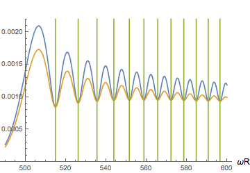
Figure 2: Plot of the magnitudes of ${\rm Det_{TM}}(\omega R)$ (blue curve) and ${\rm Det_{TE}}(\omega R)$ (brown curve) as a function of $\omega R$ for $l=500$. The refractive indices are $n_{1}=1.0$, $n_{2}=1.1$. The green lines are the locations of the first few zeros of ${\rm J}_{l}(n_{1}\omega R)$. The locations of the minima are the real parts of $R$ times the resonant eigenfrequencies.

Now we introduce a small $k_{z}$. The pairs of equations are now coupled, but we see that the term with $k_{z}$ on the LHS of the $E_{y}$ and $H_{y}$ continuity equations multiplies ${\rm J}_{l}(x)$, and this quantity is small at resonance. We therefore neglect these terms. If we look at the $E_{x}$ and $H_{x}$ continuity equations (whose validity was previously enforced by the others) and neglect the RHS radiation fields, we find that the eigenvalue equations simplify to

$$k_{z}n_{1}\omega{\rm J^{\prime}}_{l}(n_{1}\omega R)A-{il\omega\over R}{\rm J}_{l}(n_{1}\omega R)C = 0,$$

$$k_{z}n_{1}\omega{\rm J^{\prime}}_{l}(n_{1}\omega R)C+{il\omega n^{2}\over R}{\rm J}_{l}(n_{1}\omega R)A = 0.$$ (41)

As we are very close to zeros of the Bessel function, we can set ${\rm J}_{l}(z_{l,n}+n_{1}\delta\omega R)\approx n_{1}R\,{\rm J^{\prime}}_{l}(z_{l,n})\,\delta\omega$ and (41) reduce to

$$k_{z}A-il\,\delta\omega\,C = 0,$$

$$k_{z}C+iln_{1}^{2}\,\delta\omega\,A = 0.$$ (42)

These two equations coincide once we set $(A,C)=(1,\pm in_{1})$, which corresponds to right and left circularly polarized light in a medium of refractive index $n_{1}$. They give a frequency shift of

$$\delta\omega=\pm{1\over ln_{1}}k_{z}.$$ (43)

The longitudinal group velocity of a wave packet centered around $k_{z}=0$ s therefore

$$\dot{z}\equiv{\partial\omega\over\partial k_{z}}=\pm{1\over n_{1}l}.$$ (44)

Since $n_{1}\omega R\sim l$ for these modes and $n_{1}\omega=k_{\phi}$ is the wavenumber for the light in the core, we can write this equation as

$$\dot{z}=\pm{1\over n_{1}k_{\phi}R}=\pm{\lambda_{\rm glass}\over 2\pi n_{1}R}$$ (45)

where $\lambda_{\rm glass}$ is the wavelength of the light in the fibre core. As the time for one orbit is $2\pi Rn_{1}$, we find that the rate of drift is one (in glass) wavelength per orbit. This is exactly what we expect from the berry phase argument in section II. The photons can only make a few orbits, however, before they escape or become depolarized due to the TE mode (which, looking along the circumferential ray, is a linearly polarized beam with the ${\bf E}$ field in the radial direction) having a shorter lifetime that the TM (which is a linearly polarized beam with the ${\bf E}$ field in the $z$ direction).

In an actual fibre we have $n_{1}>n_{2}$. In this regime the Bessel function ${\rm J}_{l}(n_{1}\omega r)$ begins to oscillate while the Hankel function ${\rm H}^{(1)}_{l}(n_{2}\omega r)$ is still almost real and exponentially decreasing. In the region of $\omega R$ corresponding to total internal reflection, the fields outside the glass decay almost to zero as they would for total internal reflection off a flat interface — but eventually the Hankel function begins to oscillate and the fields become outgoing radiation.

We assume that $k_{z}$ is small, so that we can ignore the $k_{z}$’s in $\gamma_{1}$ and $\gamma_{2}$. The boundary condition equations are then

$$\left({ik_{z}l\over R}{1\over\epsilon_{1}\mu_{1}}\,{\rm J}_{l}(\gamma_{1}R)C-\omega^{2}\sqrt{{\epsilon_{1}\over\mu_{1}}}{\rm J^{\prime}}_{l}(\gamma_{1}R)\,A\right) = \left({ik_{z}l\over R}{1\over\epsilon_{2}\mu_{2}}\,{\rm H}_{l}^{(1)}(\gamma_{2}R)D-\omega^{2}\sqrt{{\epsilon_{2}\over\mu_{2}}}{{\rm H}^{\prime}}_{l}^{(1)}(\gamma_{2}R)\,B\right)$$

$${\rm J}_{l}(\gamma_{1}R)\,A = {\rm H}^{(1)}_{l}(\gamma_{2}R)\,B$$

$$\left({ik_{z}l\over R}{1\over\epsilon_{1}\mu_{1}}\,{\rm J}_{l}(\gamma_{1}R)A-\omega^{2}\sqrt{{{\mu}_{1}\over\epsilon}_{1}}{\rm J^{\prime}}_{l}(\gamma_{1}R)\,C\right) = \left({ik_{z}l\over R}{1\over\epsilon_{2}\mu_{2}}\,{\rm H}_{l}^{(1)}(\gamma_{2}R)B-\omega^{2}\sqrt{{\mu_{2}\over\epsilon_{2}}}{{\rm H}^{\prime}}_{l}^{(1)}(\gamma_{2}R)\,D\right).$$

$${\rm J}_{l}(\gamma_{1}R)\,C = {\rm H}^{(1)}_{l}(\gamma_{2}R)\,D$$ (46)

From now on we make the assumption that the impedance does not change from core to cladding— I.e. that $\sqrt{{\mu_{1}}/{\epsilon_{1}}}=\sqrt{{\mu_{2}}/{\epsilon_{2}}}$. This impedence matching condition might be hard to engineer, but given that we are seeking a mathematical illustration of the anomalous-velocity equation rather than proposing experimental verification it is not unreasonable. The matching means that the right and left handed Riemann Silberstein fields do not mix. It also ensures the degeneracy of the $k_{z}=0$ TE and TM modes, both eigenfrequences being determined by the same vanishing condition

$${\rm Det}(\omega R)\equiv{\rm J^{\prime}}_{l}(n_{1}\omega R){\rm H}_{l}^{(1)}(n_{2}\omega R)-{\rm H^{\prime}}^{(1)}(n_{2}\omega R){\rm J}_{l}(n_{1}\omega R)=0.$$

See figure 3 for a plot that locates the zeros of ${\rm Det}(\omega R)$.

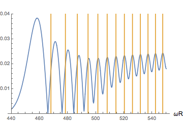
Figure 3: Plot of the magnitude of ${\rm Det}(\omega R)/{\rm H}_{l}^{(1)}(n_{2}\omega R)$ (blue curve) against $\omega R$ for an impedance-matched fibre with $n_{1}=1.1$, $n_{2}=1$ and $l=500$. The brown lines are the locations of the first few zeros of ${\rm J}_{l}(n_{1}\omega R)$. The three deep minima are resonances in the high-$Q$ total-internal-reflection region. The minima become shallower once the angle of incidence of the rays decreases below the critical angle, allowing the light to leak out and the eigen-frequencies to acquire a significant imaginary part.

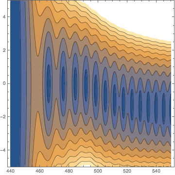
Figure 4: Contour plot (blue is lowest value) of the magnitude of ${\rm Det}(\omega R)/{\rm H}_{l}^{(1)}(n_{2}\omega R)$ In the complex $\omega R$ plane for the same range of parameters as figure 3. The first three zeros lie very close to the real axis. They correspond to modes that are strongly confined by total internal reflection. The remaining zeros break away from the axis and their larger imaginary parts indicate that the light rays can escape because they are below the critical angle.

For non-zero $k_{z}$ the TE and TM pairs of equations are again coupled, but, accepting the impedance-matching condition we can decouple the four equations into a different two pairs of equations — one for each helicity. We set

$$(A,C) = (1,i\sqrt{\epsilon_{1}/\mu_{1}})X_{+}$$

$$(B,D) = (1,i\sqrt{\epsilon_{2}/\mu_{2}})Y_{+}$$ (47)

and similarly, with the sign before the $i$ changed, for $X_{-}$, $Y_{-}$. Using the notation $c_{1,2}=1/n_{1,2}$, the equations for the “+” pair become

$$\left({k_{z}l\over R}c_{1}^{2}{\rm J}_{l}(\omega R/c_{1})+\omega^{2}{\rm J^{\prime}}_{l}(\omega R/c_{1})\right)X_{+} = \left({k_{z}l\over R}{c_{2}}^{2}{\rm H}_{l}^{(1)}(\omega R/c_{2})+\omega^{2}{{\rm H}^{\prime}}_{l}^{(1)}(\omega R/c_{2})\right)Y_{+}$$

$${\rm J}_{l}(\omega R/c_{1})X_{+} = {\rm H}_{l}^{(1)}(\omega R/c_{2})Y_{+}$$ (48)

Dividing the first by the second equation and rearranging gives

$${k_{z}l\over R}(c_{1}^{2}-{c_{2}}^{2})=\omega^{2}\left({{\rm J^{\prime}}_{l}(\omega R/c_{1})\over{\rm J}_{l}(\omega R/c_{1})}-{{{\rm H}^{\prime}}_{l}^{(1)}(\omega R/c_{2})\over{\rm H}_{l}^{(1)}(\omega R/c_{2})}\right).$$ (49)

When $k_{z}=0$ the vanishing of the RHS is the eigenvalue condition. To find $\partial\omega/\partial k_{z}$ at $k_{z}=0$, we therefore need to compute the derivative of the RHS at the points at which it vanishes. To do this we make use of the asymptotic formula

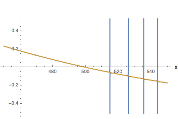
Figure 5: Plot of ${\rm J}^{\prime\prime}_{l}(x)/{\rm J}_{l}(x)$ (blue curve) compared with $l^{2}/x^{2}-1$ (brown curve) for $l=500$. The brown curve sits on top of the blue curve except for the spikes near the zeros of ${\rm J}_{l}(x)$.

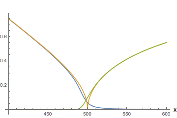
Figure 6: Plot of the real (blue curve) and imaginary parts (green curve) of $\,{\rm H^{\prime}}^{(1)}_{l}(x)/{\rm H}^{(1)}_{l}(x)$ compared with $\sqrt{|1-l^{2}/x^{2}|}$ (brown curve) for $l=500$.

$${{\rm J}^{\prime\prime}_{l}(x)\over{\rm J}_{l}(x)}\sim{l^{2}\over x^{2}}-1\\$$

which is accurate for large $x$ provided that we stay away from places where ${\rm J}_{l}(x)$ vanishes [see figure 5]. This condition is satisfied at the points of interest [see figure 3]. We may also use the formulæ

$${{{\rm H}^{\prime\prime}}_{l}^{(1)}(x)\over{\rm H}_{l}^{(1)}(x)} \sim {l^{2}\over x^{2}}-1$$

$${{{\rm H}^{\prime}}_{l}^{(1)}(x)\over{\rm H}_{l}^{(1)}(x)} \sim -\sqrt{{l^{2}\over x^{2}}-1},\quad x<l.$$ (50)

These last two approximations [see figure 6] imply that

$$\left({{\rm H}^{\prime}\over\rm H}\right)^{\prime}={{\rm H}^{\prime\prime}\over\rm H}-\left({{\rm H}^{\prime}\over\rm H}\right)^{2}\sim 0,$$ (51)

which is not quite right, but the derivative on the LHS is $O(1/l)$ in the region of interest and can be neglected. We also note that we can evaluate

$$\left({{\rm J}^{\prime}_{l}(x)\over{\rm J}_{l}(x)}\right)^{\prime}={{\rm J}_{l}^{\prime\prime}(x)\over{\rm J}_{l}(x)}-\left({{\rm J}_{l}^{\prime}(x)\over{\rm J}_{l}(x)}\right)^{2}$$ (52)

at the unperturbed eigenvalue by exploiting the fact that ${\rm J}_{l}^{\prime}/{\rm J}_{l}={\rm H}^{\prime}_{l}/{\rm H}_{l}$ at that point. We find

$${l\over R}(c_{1}^{2}-{c_{2}}^{2})\delta k_{z} = {\omega^{2}R\over c_{1}}\left[\left({l^{2}c_{1}^{2}\over\omega^{2}R^{2}}-1\right)-\left({l^{2}c_{2}^{2}\over\omega^{2}R^{2}}-1\right)\right]\delta\omega$$ (53)

$$= {\omega^{2}R\over c_{1}}\left[{l^{2}(c_{1}^{2}-{c_{2}}^{2})\over\omega^{2}R^{2}}\right]\delta\omega.$$

Thus

$$\delta\omega={c_{1}\over l}\delta k_{z}={c\over n_{1}l}\,\delta k_{z}.$$ (54)

The opposite circularly-polarized have an opposite frequency shift. We have therefore recovered the same drift equation

$$\dot{z}={\partial\omega\over\partial k_{z}}=\pm{c\over n_{1}l}$$ (55)

that we found for the $n_{1}<n_{2}$ fibre. Recall that this drift is at a rate of one wavelength per orbit.

IV Discussion

We can compare the mode-expansion rate of drift with that expected from angular momentum conservation about an axis perpendicular to the reflection interface. For a particle of momentum ${\bf p}$ and helicity $S$, and treating the orbit as a series of grazing-angle reflections, each deflection through an angle $\delta\phi$ causes a change in the perpendicular spin component of $2S\sin(\delta\phi/2)$ that must be compensated for by a change in the orbital angular momentum of $-|{\bf p}|\delta z$. Thus $|{\bf p}|\dot{z}=-S\dot{\phi}$. Since $\dot{\phi}R=c/n_{\rm glass}$ we have

$$\dot{z}=-S{c\over n_{\rm glass}|{\bf p}|R}.$$ (56)

In this picture the drift may be understood as a continuous version of the Imbert-Fedorov effect [19, 18].

Agreement with the results of the previous section requires us to identify the magnitude of the photon momentum $|{\bf p}|$ with $2\pi\hbar/\lambda_{\rm glass}=n_{\rm glass}\hbar\omega/c$, This is the Minkowski expression for the momentum of a photon in a medium — as opposed to Abraham’s expression for the momentum which places the $n_{\rm glass}$ in the denominator. (For a review the Abraham-Minkowski momentum controversy see [21].) Minkowski’s momentum is today understood to be the pseudo-momentum which is conserved as a result of the homogeneity of the medium [20]. It is the rotational symmetry of the medium about the normal to the core-cladding interface that is responsible for the angular momentum conservation, so the appearance of the Minkowski momentum is not surprising.

That a continuous process of reflection and rotation can transport a circularly polarized beam of light parallel to itself through an arbitrary distance is related to the fact that a continuous sequence of Lorentz boosts and rotations in free space can perform an arbitrary “Wigner translation” of a finite polarized beam [22].

V Acknowledgements

This project was supported by the National Science Foundation under grant NSF DMR 13-06011. I would like to thank Konstantin Bliokh and Misha Stephanov for e-mail discussions.

VI Appendix: Gordon decomposition, the Weyl magnetic moment, and $g=2$.

The orginal Gordon decomposition of the Dirac 4-current [23] shows that for any solution $\psi$ of the massive Dirac equation

$$(i\gamma^{\mu}(\nabla_{\mu}-m)\psi=0,$$ (57)

the four-current can be expressed as

$$\bar{\psi}\gamma^{\mu}\psi={i\over 2m}(\bar{\psi}\nabla^{\mu}\psi-(\nabla^{\mu}\bar{\psi})\psi)+{1\over m}\partial_{\nu}(\bar{\psi}\Sigma^{\mu\nu}\psi),$$ (58)

where

$$\Sigma^{\mu\nu}={i\over 4}[\gamma^{\mu},\gamma^{\nu}]$$ (59)

is the Lorentz generator.

Gordon’s decomposition of the current into a particle number-flux and bound spin contribution clearly requires $m\neq 0$. There is, however, a version that is valid in both massive and massless cases: assume that $\psi({\bf r},t)=\psi({\bf r})\exp\{-iEt\}$ and make use of the Dirac equation in the Hamiltonian form

$$\partial_{t}\psi = -{\mbox{\boldmath$\alpha$}}\cdot\nabla\psi-im\beta\psi,$$

$$\partial_{t}\bar{\psi} = +\nabla\bar{\psi}\cdot{\mbox{\boldmath$\alpha$}}+im\bar{\psi}\beta,$$

with $\beta=\gamma^{0}$, $\alpha^{i}=\gamma^{0}\gamma^{i}$ and so find

$${\bf j}\equiv e\bar{\psi}{\mbox{\boldmath$\gamma$}}\psi={e\over 2iE}\left(\psi^{\dagger}\nabla\psi-(\nabla\psi^{\dagger})\psi\right)+{e\over E}(\nabla\times{\bf S}).$$ (60)

Here ${\mbox{\boldmath$\gamma$}}=(\gamma^{1},\gamma^{2},\gamma^{3})$, and

$${\bf S}=\psi^{\dagger}\hat{\bf S}\psi$$ (61)

with

$$(\hat{S}_{x},\hat{S}_{y},\hat{S}_{z})=(\Sigma^{23},\Sigma^{31},\Sigma^{12})$$ (62)

so that

$$\hat{\bf S}={1\over 2}\left[\begin{matrix}{\mbox{\boldmath$\sigma$}}&0\cr 0&{\mbox{\boldmath$\sigma$}}\end{matrix}\right].$$ (63)

With the particle-number density identified with $\rho=\psi^{\dagger}\psi$, we can again interpret the first term in the decomposition as the current ${\bf j}_{\rm free}=e\rho{\bf k}/E=e\rho{\bf v}$ due to particles moving at speed ${\bf v}={\bf k}/E$. The second term, ${\bf j}_{\rm bound}=(e/E)\nabla\times{\bf S}$ is the current due to the gradients in the intrinsic magnetic moment density. The magnetic moment itself is found by integrating by parts to show that

$${\mbox{\boldmath$\mu$}}\stackrel{{\scriptstyle\rm}}{{=}}{1\over 2}\int{\bf r}\times{\bf j}_{\rm bound}\,d^{3}x={1\over 2}\int{\bf r}\times\left({e\over E}\nabla\times{\bf S}\right)\,d^{3}x={e\over E}\int{\bf S}\,d^{3}x.$$ (64)

For a single massless particle whose spin-1/2 is locked to the direction $\hat{\bf k}$ of its kinetic momentum this is

$${\mbox{\boldmath$\mu$}}_{\rm Weyl}={e\hat{\bf k}\over 2E},$$ (65)

as claimed in section II.

For the both massive and massless case we also have an expression for the momentum density as part of the symmetric Belinfante-Rosenfeld energy-momentum tensor

$$T^{\mu\nu}_{\rm BR}={i\over 4}(\bar{\psi}\gamma^{\mu}\nabla^{\nu}\psi-(\nabla^{\nu}\bar{\psi})\gamma^{\mu}\psi+\bar{\psi}\gamma^{\nu}\nabla^{\mu}\psi-(\nabla^{\mu}\bar{\psi})\gamma^{\nu}\psi).$$ (66)

Using the Dirac equation we evaluate $T^{0\mu}_{\rm BR}=({\mathcal{E}},{\bf P})$ to find ${\mathcal{E}}=E\psi^{\dagger}\psi$, and

$${\bf P}={1\over 2i}\left(\psi^{\dagger}(\nabla\psi)-(\nabla\psi^{\dagger})\psi\right)+{1\over 2}\nabla\times{\bf S}.$$ (67)

(If we used the non-symmetric canonical energy-momentum tensor

$$T^{\mu\nu}_{\rm canonical}={i\over 2}(\bar{\psi}\gamma^{\mu}\nabla^{\nu}\psi-(\nabla^{\nu}\bar{\psi})\gamma^{\mu}\psi),$$ (68)

we do would not find the bound spin-momentum contribution.)

Again integrating by parts, we recover the spin contribution to the total angular momentum density as

$$\int{\bf r}\times\left({1\over 2}\nabla\times{\bf S}\right)\,d^{3}x=\int{\bf S}\,d^{3}x,$$ (69)

so the division by 2 in the spin contribution to the momentum density is correct. The absence of a division by 2 in the formula for the current reflects the $g=2$ gyromagnetic ratio of the electron. In other words a spin-density gradient is twice as effective at making an electric current as it is at contributing to the momentum.

References

- [1] E. N. Adams, E. I. Blount, Energy bands in the presence of an external force field II: Anomalous velocities, J. Phys. Chem. Solids, 10 286-303 (1959); E. I. Blount in Solid State Physics, edited by F. Seitz and D. Turnbull (Academic Press New York, 1962) Vol 13, p305.
- [2] G. Sundaram, Q. Niu, Wave Packet Dynamics in Slowly Perturbed Crystals – Energy Gradient Correction and Berry Phase Effects, Phys. Rev. B59 14915-14925 (1999).
- [3] D. Xiao, J. Shi, Q. Niu, Berry Phase Correction to Electron Density of States in Solids, Phys. Rev. Lett. 95 137204 1-4 (2005).
- [4] C. Duval, Z. Horváth, P. A. Horváthy, L. Martina, P. C. Stichel, Berry Phase Correction to Electron Density in Solids, Modern Physics Letters B 20 373-378 (2006).
- [5] Y. D. Chong, Berry’s phase and the anomalous velocity of Bloch wavepackets, Phys. Rev. B 81 052303 1-2 (2010).
- [6] M. V. Berry, Quantal Phase Factors Accompanying Adiabatic Changes, Proc. Roy. Soc. Lond. A392, 45-57 (1984).
- [7] M. A. Stephanov, Y. Yin, Chiral Kinetic Theory, Phys. Rev. Lett. 109 162001 1-5 (2012).
- [8] M. Stone, V. Dwivedi, A Classical Version of the Non-Abelian Gauge Anomaly Phys. Rev. D 88 045012 1-8 (2013).
- [9] V. Dwivedi, M. Stone, Classical chiral kinetic theory and anomalies in even space-time dimensions J. Phys. A 47 025401 1-20 (2014).
- [10] A. Vilenkin, Microscopic partity violating effects: neutrino fluxes from rotating black holes amd rotating thermal radiation, Phys Rev D bf 20 1807-1812; Equilibrium parity-violating current in a magnetic field Phys. Rev. D 22 3080-3084 (1980).
- [11] K. Fukushima, D. E. Kharzeev, H. J. Warringa, Chiral magnetic effect, Phys. Rev. D 78, 074033 (2008).
- [12] J-Y. Chen, D. T. Son, M. A. Stephanov, H-U. Yee, Y. Yin, Lorentz Invariance in Chiral Kinetic Theory, Phys. Rev. Lett. 113 182302 1-5 (2014).
- [13] H. M. Weber, Die partiellen Differential-Gleichungen der mathematischen Physik nach Riemann’s Vorlesungen, p348, (Friedrich Vieweg und Sohn, Braunshweig 1901).
- [14] L. Silberstein, Elektromagnetische Grundgleichungen in bivectorieller Behandlung, Annalen der Phys. 22 579-586 (1907); Nachtrag zur Abhandlung über Elektromagnetische Grundgleichungen in bivectorieller Behandlung, Annalen der Phys. 24 783-784 (1907).
- [15] I. Białynicki-Birula, Z. Białynicki-Birula, The role of the Riemann-Silberstein vector in classical and quantum theories of electromagnetism, J. Phys. A 46 053001-32 (2013).
- [16] K. Yu. Bliokh, Yu. P. Bliokh, Modified geometrical optics of a smoothly inhomogeneous isotropic medium: The anisotropy, Berry phase, and the optical Magnus effect, Phys. Rev. E 70, 026605-9 (2004).
- [17] K. Y. Bliokh, A. Niv, V. Kleiner, E. Hasman Geometrodynamics of spinning light, Nature Photon. 2, 748-753 (2008).
- [18] F. I. Fedorov, To the theory of total reflection, Doklady Akademii Nauk SSSR 105, 465-468 (1955) [translated and reprinted in J. Opt. 15 014002-3 (2013)].
- [19] C. Imbert, Calculation and experimental proof of the transverse shift induced by total internal reflection of a circularly polarized light beam, Phys. Rev. D 5 787-796 (1972).
- [20] E. I. Blount, Bell Telephone Laboratories technical memorandum 38139-9. (1971).
- [21] R. N. C. Pfeifer, T. A. Nieminen, N. R. Heckenberg, H. Rubinsztein-Dunlop, Colloquium: Momentum of an electromagnetic wave in dielectric media, Rev. Mod. Phys. 79 1197-1216 (2007); Erratum: Rev. Mod. Phys. 81, 443 (2009).
- [22] M. Stone, V. Dwivedi, T. Zhou, Wigner Translations and the Observer Dependence of the Position of Massless Spinning Particles, Phys. Rev. Lett. 114 210402 1-4 (2015)
- [23] W. Gordon, Der Strom der Diracschen Elektronentheorie, Z. Phys. 50 630-632 (1928).