X-ray observations of the hot phase in Sgr A*

Abstract

Context. We analyze 134 ks Chandra ACIS-I observations of the Galactic Centre (GC) performed in July 2011. The X-ray image with the field of view $17^{\prime}\times 17^{\prime}$ contains the hot plasma surrounding the Sgr A*. The obtained surface brightness map allow us to fit Bondi hot accretion flow to the innermost hot plasma around the GC.

Aims. Contrary to the XMM-Newton data where strong 6.4 keV iron line was observed and interpreted as a reflection from molecular clouds, we search here for the diffuse X-ray emission with prominent 6.69 keV iron line. The surface brightness profile found by us allowed to determine the stagnation radius of the flow around Sgr A*.

Methods. We have fitted spectra from region up to $5^{\prime\prime}$ from Sgr A* using a thermal bremsstrahlung model and four Gaussian profiles responsible for K_α emission lines of Fe, S, Ar, and Ca. The X-ray surface brightness profile up to $3^{\prime\prime}$ from Sgr A* found in our data image, was successfully fitted with the dynamical model of Bondi spherical accretion.

Results. We show that the temperature of the hot plasma derived from our spectral fitting is of the order of 2.2-2.7 keV depending on the choice of background. By modelling the surface brightness profile, we derived the temperature and number density profiles in the vicinity of the black hole. The best fitted model of spherical Bondi accretion shows that this type of flow works only up to $3^{\prime\prime}$ and implies outer plasma density and temperature to be: $n_{\rm e}^{\rm out}=18.3\pm{0.1}$ cm^-3 and $T_{\rm e}^{\rm out}=3.5\pm{0.3}$ keV respectively.

Conclusions. We show that the Bondi flow can reproduce observed surface brightness profile up to $3^{\prime\prime}$ from Sgr A* in the Galactic Center. This result strongly suggests the position of stagnation radius in the complicated dynamics around GC. The temperature at the outer radius of the flow is higher by 1 keV, than this found by our spectral fitting of thermal plasma within the circle of $5^{\prime\prime}$. The Faraday rotation computed from our model towards the pulsar PSR J1745-2900 near the GC agrees with the observed one, recently reported. We speculate here, that the emission lines observed in spectra up to $5^{\prime\prime}$ can be interpreted as the reflection of the radiation from two-phase regions occurring at distances between $3-5^{\prime\prime}$ of the flow. The hot plasma in Sgr A* illuminated in the past by strong radiation field may be a seed for thermal instabilities and eventual strong clumpiness.

1 Introduction

The central region of the Milky Way hosts a supermassive black hole (BH) with well established mass $M_{\rm BH}=4.4\times 10^{6}M_{\odot}$ (Genzel et al. 2010), at a distance $R=8.4$ kpc. The surroundings of the black hole are unique. It contains a number of relatively cold molecular clouds (Zhao et al. 2009) located within $15^{\prime}$ from Sgr A*, and a hot plasma of temperature around 2 keV situated within a few arcmin (Baganoff et al. 2003). Both phases of gas show X-ray emission with prominent iron K_α line, which may arise due to reflection of hard radiation emitted at the very center of the Galaxy nucleus.

The cold phase emits neutral Fe K_α line at energy 6.4 keV, as in case of molecular clouds reported recently by Ponti et al. (2010). These cold clouds situated at the distance of 30-60 pc from the Galactic Centre (GC), are well resolved by the XMM-Newton satellite, enabling proper studies of their velocities and the nature of the reflected continuum. Tracing history of fluorescent reflection, it is possible to capture historic luminosity variations of Sgr A* (Yu et al. 2011).

The hot phase emits the Fe K_α line at energy 6.690 keV, indicating that iron atoms are in helium-like ionization state. X - ray emission from a diffuse hot gas was observed in extended regions around the GC (Park et al. 2004; Muno et al. 2004). Particularly, it appears to be concentrated within the central 2-3 pc eastwards from Sgr A*, named Sgr A East, and most probably is caused by a young supernova remnant (SNR) (Maeda et al. 2002). Additionally, the hot phase lies on the line of sight toward Sgr A* and it may accrete on supermassive black hole in the form of spherical Bondi accretion or radiatively inefficient accretion flow (RIAF). The dynamical model of the accretion on the GC is still not well established since it is clearly seen that this region may be a mixture of hot plasma with cold clouds i.e. mini-spiral region (Zhao et al. 2010). The accretion of hot plasma fed by stars due to mass and energy exchange was proposed by Shcherbakov & Baganoff (2010) to explain the observed surface brightness profile. On the other hand, Czerny et al. (2013) constructed a model of multiple accretion events caused by cold clouds to trigger the Sgr A* activity. Such hot and cold two-phase medium can be formed due to thermal instability caused by irradiation with hard X-rays from the GC, as recently shown by Różańska et al. (2014). Thermally unstable clouds can be located close to the center at 0.008-0.2 pc, i.e. within $5^{\prime\prime}$, and they can survive hundreds years. The radiation reflected from those clouds can produce hot iron line in that region.

Since the extension of the hot gas is an order of magnitude lower than of the cold phase, Chandra and Suzaku satellites are better for detailed studies of those regions (e.g. Maeda et al. 2002; Koyama et al. 2007; Wang et al. 2013, and references therein). Recently, Wang et al. (2013) have reported results of spectral fitting of the longest 3 Msec Chandra observations of the $1.5^{\prime\prime}$ circular region around Sgr A*, and the spectrum presented in this paper is the most detailed ever published. But the surface brightness profile from dynamical model is not fitted in this paper. The authors fit model spectrum computed as a thermal emission from the distribution of temperatures and densities according to the analytical formula appropriate for RIAF (see Sec. 4.2 in this paper.

The purpose of this paper is to study the hot plasma around Sgr A*. Analysing X-ray image we aim to put constraints on the physical parameters of the hot phase, which may be an important material to be a source of radiation from Sgr A*. We present archival Chandra ACIS-I observations of the GC made in July 2011 with the field of view $17^{\prime}\times 17^{\prime}$ containing both the Sgr A* and Sgr A East. The data were collected with three time intervals, very short one after another. Therefore, spectral and imaging coadding was very accurate.

From Chandra observations, we extracted spectrum from one circular region around Sgr A* with radius of $5^{\prime\prime}$. We performed detailed spectral analysis by fitting a thermal plasma with a strong K_α line from helium-like iron. Additionally, we fitted other emission lines seen in residuals form C, Ar, Ca, but the detection of last two was marginal. Following Shcherbakov & Baganoff (2010), we extracted surface brightness profile around Sgr A* within the radius of $10^{\prime\prime}$ with sub-pixel accuracy. We fitted the dynamical model of the hot Bondi accretion flow by Mościbrodzka et al. (2009) to this imaged emissivity profile. To make a fit, for each computed model we constructed the map of emission around GC convolved with Chandra exposure map of ACIS-I chip. In our observations Sgr A* is located off-axies, and we constructed point spread function (PSF) to account for this particular observation. Final models were convolved with normalized PSF, before comparing to the data. We point out here, that only basic spectral fitting is done in this paper due to the short time exposure. In contrast to Wang et al. (2013), we do not compute the line emissivity from our model. Instead, we focus on modeling the sub-pixel surface brightness profile (see also Shcherbakov & Baganoff 2010).

The main result of the observed surface brightness profile modelling is the derivation of electron density and temperature profiles of the flow from $3^{\prime\prime}$ down to the black hole horizon. The best fitting model is for temperature and density at the outer flow radius $T_{\rm e}^{\rm out}=3.5\pm 0.3$ keV, and $n_{\rm e}^{\rm out}=18.3\pm 0.1$ cm^-3. Our fit is not valid outside $3^{\prime\prime}$ indicating the location of the stagnation radius of the dynamical flow around GC. Ouside stagnation radius, matter can possess outflow as it was indicated in RIAF model of Wang et al. (2013). The temperature at the outer flow radius is in good agreement with that derived from spatially resolved spectral modelling presented in Wang et al. (2013), and then rejected by RIAF model. In addition, Wang et al. (2013) considered RIAF model, where the line emissivity was computed from the predicted RIAF temperature profile. Such line fitted to the data indicated the outer plasma temperature to be 1 keV, which is lower than in our model. In this paper we compare temperature and density profiles implied for both models, RIAF and Bondi.

Fitting the canonical model of thermal bremsstrahlung plus Gaussian profiles for all lines indicates temperatures for the plasma around Sgr A* in the 2.2–2.7 keV range, depending on the choice of background. And again, those values are lower than that obtained by Wang et al. (2013) with the same model for the $1.5^{\prime\prime}$ Sgr A* spectral fitting, but higher then 1 keV temperature derived by them using RIAF emissivity profile. The EW of the iron line we find is in the $0.9-1.2$ keV range. Within the uncertainties, our EW of the iron line is consistent with that estimated by Wang et al. (2013) at the $1\sigma$ confidence level. Since the result is degenerated according to plasma temperature and warm absorption, the broad-band spectra are needed to discriminate between models.

In addition, we calculated the Faraday rotation (RM) towards the Galactic Center and towards the pulsar located at $3^{\prime\prime}$ in the projected distance away from the GC. The first result matches with observations (Marrone et al. 2007) only with additional assumption of the very weak magnetic field, while the second result agrees with the recently observed value very well (Eatough et al. 2013).

Our paper shows that Bondi accretion can well represent the hot phase accretion on the GC up to $3^{\prime\prime}$. We argue that the radiation originating from the very close vicinity of Sgr A*, illuminating external zones of the Bondi flow may produce two-phase medium when all lines are created. The exact distance of such clumps and their lifetime are given in Różańska et al. (2014). The temperature of such clouds varies from log$(T)=5.5-7.5$ in Kelvins, and the warm clouds have longer lifetimes than the cold clouds. We postulate here, that they can be responsible for the formation of iron line at energy 6.7 keV, seen in the Chandra data. Better data are needed to fully confirm this hypothesis.

The structure of the paper is as follows: in Sec. 2 we present the details of data extraction that resulted in obtaining images, brightness profile and spectra of hot plasma in the neighbourhood of the GC. Sec. 3 contains results of spectral fitting, while Sec. 4 shows results of surface brightness profile fitting in the vicinity of Sgr A*. Discussion and conclusions are presented in Sec. 5.

2 Observations

The Chandra X-Ray Observatory has observed the central regions of the Galaxy multiple times. For our analysis, we have selected three observations carried out in July 2011. the longest unpublished observations available in the Chandra archive. They were performed for a very similar period of time, allowing to avoid significant changes with time and astrometry. Table 1 presents identification numbers, starting dates and exposure times of the observations. All of them were done using ACIS-I spectrometer with the field of view 17’ $\times$ 17’. It corresponds to the region of 40 $\times$ 40 pc in the center of our Galaxy. The pointing coordinates were $\alpha=17^{\textrm{h}}45^{\textrm{m}}59.^{\textrm{s}}70$, $\delta=-28^{\circ}58^{\prime}15.^{\prime\prime}9$, and were $4.^{\prime}8$ away from Sgr A*.

Table 1: Chandra satellite observation log.

ObsID	Date	Exp. time	GTI
		[ks]	[ks]
12949	2011-07-21	58.48	48.88
13438	2011-07-29	66.18	59.79
13508	2011-07-19	31.49	26.10

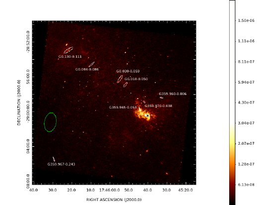
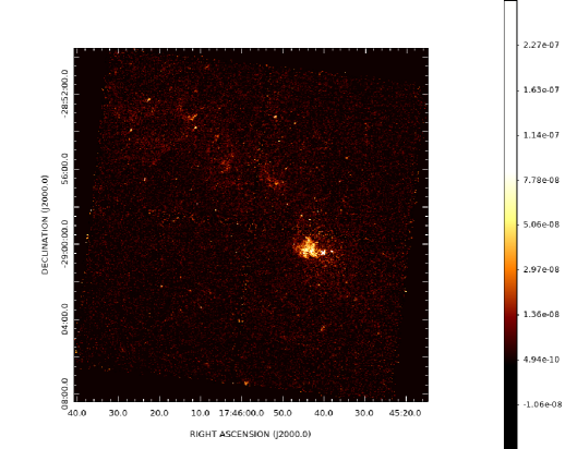
Figure 1: Flux image of the GC in the 0.5-8 keV energy range (upper panel). Sgr A* is marked with a black cross. A few brightest filaments reported by Johnson et al. (2009) are marked with white (small) ellipses and named following the names given in previous detection . The green (large) ellipse shows the region used for background spectrum extraction (the case of distant background, see Sec. 2.4 for details). Bottom panel shows flux image of the GC in the energy range of 6.3-7.0 keV, where iron line is created. Emission presented here is the K_α line emission after subtracting the continuum flux. The flux is presented in asinh scale, since it behaves well for negative count rate values which might originate during subtraction process.

2.1 Data reduction

All subsequent analysis was performed using CIAO 4.4 software, and CALDB version 4.5.3.

We started our analysis by processing individual observations. The corrections for charge transfer inefficiency, bad pixel removal, and background flaring were done in the whole energy band, 0.5-8.0 keV. The lc_sigma_clip tool was used to clip the data that deviates from the mean by more than 2 sigma. In order to minimize the influence of the molecular clouds variability we made two tests: i) point sources were removed from the ACIS-I2 CCD chip, where diffuse emission was marginal, filtering counts to the 0.5-8 keV energy band ii) photons with energy from 7 to 10 keV in the whole ACIS-I field of view were considered. In both cases similar good time intervals (GTI) were obtained. Hereinafter, we decided to use GTI found in case (i), as they set more stringent limits. For all observations the light curves are of good quality and the background flaring is insignificant. Finally, we choose GTI=134.77 ks, which covers 86% of the total exposure time.

Although during all observations the telescope was pointed at the same target, we have found a small shift between three images (a few arcsec). In order to correct the absolute astrometry of the data, we searched for point sources using the wavdetect tool. 53 bright sources were found and their coordinates were obtained from the SIMBAD astronomical database . Subsequently we have applied minor corrections to the WCS using the reproject_aspect script, which calculates shift between the wavdetect output and the absolute coordinates from a catalog.

2.2 Images in continuum and in K_α iron line bandpass

We have regraded event files to a common tangent point with reproject_events and we have merged them using dmmerge. Similar procedure was applied to the images, beside that the reproject_image and dmimgcalc scripts were used instead. We have created exposure-corrected image in the 0.5-8 keV energy band using the fluximage script. The flux image is presented in Fig. 1 upper panel, with the position of Sgr A* marked by the black cross. At this figure we have also indicated and named the brightest filaments reported by Johnson et al. (2009). Nevertheless, our total exposure time was too short to make spectral analysis of these filaments or discover new ones, so we do not proceed with their analysis. However, by merging the three observations we obtained enough counts to study the hot extended plasma around Sgr A*. Since Chandra X-ray observatory has the best spatial resolution among all currently working satellites, in Sec. 4 we present analysis of the surface brightness profile around Sgr A* with $1^{\prime\prime}$ scale resolution.

Since we were interested in the spatial distribution of the ionized iron K_α line, additional images were created in the 4.5-6.3 keV (the continuum) and 6.3-7.0 keV (broad line) energy bands. The former was subtracted from the line image with a normalization factor of 0.12. This constant was calculated on the assumption that the continuum emission is modelled by an absorbed power-law function with photon index $\Gamma=3$ and hydrogen column density $N_{\rm H}=10^{23}\ \textrm{cm}^{-2}$. The continuum spectrum was modeled using Sherpa (Freeman et al. 2001) and simulated with the fake_pha command. The response matrix and effective area files were created with mkacisrmf and mkwarf (sample RMFs and ARFs were also taken from CALDB, similar value was obtained). The normalization factor is simply the ratio of the flux in the line to the flux in the continuum energy band.

The image in iron line emission after subtracting continuum image is presented in the bottom panel of Fig. 1. The majority of point sources and diffuse emission around Sgr A* are properly subtracted. Some faint molecular clouds remained after subtraction because the emission from the cold Fe line overlaps broad line energy band (Ponti et al. 2010). We have constructed the flux image in K_β line, but the emission was negligible.

Fig. 1 bottom panel is presented in the asinh (the inverse hyperbolic sine) scale. In case of the high count rate this scale is practically logarithmic; for low values it changes linearly. It is especially useful in subtracted images i.e. the iron line, as it behaves well for negative count rate values which might be present.

2.3 Sgr A* surface brightness profile

The surface brightness profile can be constructed in counts per pixel squared as a function of distance from the BH. It was previously done for much longer observations (Shcherbakov & Baganoff 2010) with the exposure time 953 ks.

Here, we repeat this analysis for our data, but we fit them with a different model (see below Sec. 4). The size of Chandra pixel is $0.5^{\prime\prime}$, but the position of the satellite over the duration of observation can be determined with the $0.1^{\prime\prime}$ accuracy by comparing with the known positions of bright point sources. As noted by Shcherbakov & Baganoff (2010) we can achieve the pixel resolution accuracy in the surface brightness profile from knowing the orientation of the detector pixels at the given time.

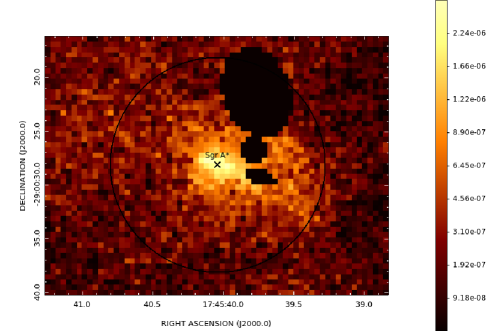
Figure 2: X-ray image of the $10^{\prime\prime}$ region around Sgr A* (circle). Surface brightness profile was extracted integrating counts over annuli from 0 to $10^{\prime\prime}$. The influence of point sources was rejected as shown in the image.

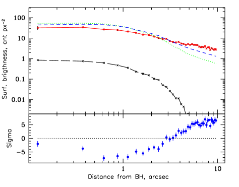
Figure 3: Vicinity of the black hole up to $10^{\prime\prime}$ from Sgr A*. Red points with errors represent observed profile, and are connected by continuous line. Black long dashed line is normalized PSF. Two models convolved with PSF are also presented: green dotted line for $T_{\rm e}^{\rm out}=1$ keV, while blue short dashed line for $T_{\rm e}^{\rm out}=3.5$ keV. Residuals are shown for best fitted model in the range up to $10^{\prime\prime}$, i.e. for $T_{\rm e}^{\rm out}=3.5$ keV.

In Fig. 2 we show pixel image of the close vicinity of the GC. It was necessary to exclude some point-like features in the Sgr A* neighbourhood because they broke spherical symmetry around the source. In order to obtain a radial profile, the net counts in a set of concentric annuli around Sgr A* were measured with dmextract tool. The width of annuli is $0.25^{\prime\prime}$, the radius of the outer annulus is $10^{\prime\prime}$, and is marked in Fig. 2 by a black circle.

The radial profile is monotonically decreasing in the whole range of radii. The final profile of the surface brightness with errors is presented in Fig. 3 by red points.

To make any further analysis of the brightness profile on the sub-pixel scale, we have to account for the point spread function (PSF) appropriate for the Chandra X-ray telescope. Any model fitted to the profile has to be convolved with the PSF. To construct the ACIS-I PSF for our observation we used the Chandra ray-tracing program, ChaRT, to simulate the Sgr A* (point source) photons scattered by the Chandra mirrors, and the MARX software version 4.5.0 to projects the simulated rays onto the detector plane. The MARX output was used to extract the PSF profile for convolution with our model spectra. ChaRT requires the position of the point source on the chip, exposure time and the point source spectrum to run the simulations. For these we used the position of Sgr A* in our stacked observation, total GTI exposure, and the best fitting model to the innermost region of Sgr A* (5”, Table 2). The normalized PSF constructed for our particular observation is presented in Fig. 3 by black crosses and long dashed line. The PSF is wider than in the paper by Shcherbakov & Baganoff (2010), due to the fact that in our observations Sgr A* was slightly off-axis.

2.4 Extraction of the spectrum

We have extracted spectra from regions where the emission of the line was the highest, especially from the region around Sgr A*. Sgr A East region is treated separately and it will be presented in the forthcoming paper.

Table 2: Best fit parameters for the $5^{\prime\prime}$ region around SgrA*. We present two cases modelled with two different statistics: CSTAT for the case where source and background are fitted simultaneously, and $\chi^{2}$ for background subtracted analysis. In the second case we consider two background regions: a distant background marked with the green ellipse in the upper panel of Fig. 1, and a local background defined as an annulus between $6^{\prime\prime}-18^{\prime\prime}$ around the $5^{\prime\prime}$ source region. In the first row we show results obtained with a model consisting of thermal bremsstrahlung with Galactic absorption (tbabs) and Fe Gaussian line only. The second row shows model parameters when three more Gaussian lines are added to account for S, Ar, and Ca emission. Both fits were done using CSTAT statistic. The third and fourth rows describe background subtracted analysis (using the local and distant backgrounds, respectively) performed on data grouped according to S/N = 3 using the $\chi^{2}$ statistic.

Bkgr.	NH	kT [keV]	Line	EKα [keV]	Line	EKα [keV]	Line	EKα [keV]	Line	EKα [keV]	Stat.	d.o.f.
Reg.	$10^{22}$ cm-2			EW [keV]		EW [keV]		EW [keV]		EW [keV]	Val.
	7.44${}^{+0.15}_{-0.15}$	3.57${}^{+0.08}_{-0.09}$	Fe	6.728${}^{+0.035}_{-0.032}$		—		—		—	CSTAT
Distant
				$0.58\pm 0.06$							1759	1019
	9.15${}^{+0.27}_{-0.25}$	2.66${}^{+0.07}_{-0.07}$	Fe	6.739${}^{+0.064}_{-0.042}$	S	2.480${}^{+0.0299}_{-0.0319}$	Ar	3.153${}^{+0.05}_{-0.03}$	Ca	3.861	CSTAT
Distant
				$0.91^{+0.40}_{-0.24}$		0.18${}^{+0.04}_{-0.05}$		0.05${}^{+0.02}_{-0.02}$		0.03${}^{+0.02}_{-0.01}$	1254	1008
	10.52${}^{+0.42}_{-0.39}$	2.24${}^{+0.07}_{-0.07}$	Fe	6.745${}^{+0.118}_{-0.069}$	S	2.489${}^{+0.030}_{-0.030}$	Ar	3.215${}^{---}_{---}$	Ca	3.865${}^{---}_{---}$	$\chi^{2}$
Local
				$1.19^{+0.89}_{-0.48}$		0.20${}^{+0.09}_{-0.09}$		0.06${}^{+0.04}_{-0.03}$		0.05${}^{+0.04}_{-0.03}$	117.32	208
	9.45${}^{+0.31}_{-0.27}$	2.58${}^{+0.07}_{-0.09}$	Fe	6.731${}^{+0.064}_{-0.045}$	S	2.488${}^{+0.012}_{-0.028}$	Ar	3.140${}^{+0.059}_{-0.040}$	Ca	3.866${}^{+0.055}_{-0.086}$	$\chi^{2}$
Distant
				$0.92^{+0.32}_{-0.26}$		0.21${}^{+0.06}_{-0.06}$		0.06${}^{+0.03}_{-0.03}$		0.04${}^{+0.03}_{-0.02}$	122.64	198

For the purpose of this work, spectrum from circular region of the radius of $5^{\prime\prime}$ around Sgr A* was extracted and analysed in details. This was done to see how far from the BH the iron line emission is crucial, and to estimate the temperature at the outer radius of the dynamical flow, which is independently derived while the surface brightness profile is fitted as presented in Sec. 4.1.

Prior to creating the spectrum, a few point-like sources were excluded since they might contaminate the results. The spectrum was obtained with the specextract script for each observation independently and merged with the combine_spectra tool. We consider two different regions for background: a distant region marked as a green ellipse in the upper panel of Fig. 1, and a local region defined as an annulus between $6^{\prime\prime}-18^{\prime\prime}$ around the $5^{\prime\prime}$ source region. The distant background region does not contain any point sources, and the diffuse emission is negligible inside the ellipse. In the case of local background the possible point source contamination was investigated and corrected for during the data reduction process. After background subtraction, the $5^{\prime\prime}$ source photon’s number in the 0.5-8 keV band is equaled to 2937 and 2358, for case distant and local backgrounds, respectively. Full description of our spectral analysis is presented below in Sec. 3.

3 Spectral fitting

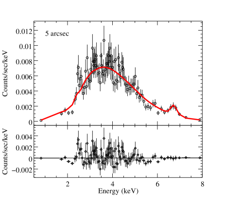
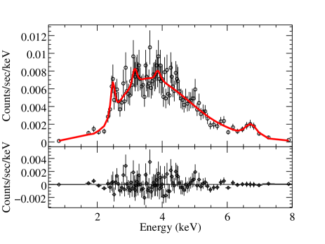
Figure 4: Modelling of the spectrum extracted from the $5^{\prime\prime}$ circular region around the Sgr A*. Both panels present fits with distant background. The upper panel shows a model consisting of Galactic absorption (tbabs), thermal bremsstrahlung and one Gaussian line to account for the iron emission. The lower panel shows a model with three additional Gaussian lines for the S, Ar and Ca emission.

The spectral fitting of the data was performed with the Sherpa 4.4 fitting package. In all plots presented in this section, the data were grouped requiring the signal-to-noise ratio $S/N=5$, for presentation purposes only. All errors on the spectral parameters correspond to the 68% confidence level (1$\sigma$) for one significant parameter.

In the first step, considering case A (distant background), we rejected simple background subtraction process. Instead, the source region and corresponding background were modelled simultaneously using the CSTAT statistic. We used a phenomenological model composed of a thermal bremsstrahlung emission (bremss) to describe the continuum, and a Gaussian profile to account for the iron K_α line emission. The total model was multiplied by warm Galactic absorption (tbabs). The background data were parametrized with a power law model. Resulting fit parameters are presented in Tab. 2 in the first row. Figure 4 (upper panel) shows the data and the best fit model together with residuals. The fit resulted in CSTAT=1759 for 1019 degrees of freedom (d.o.f.). The residuals below 4 keV hint at the presence of additional emission lines detected e.g. by Wang et al. (2013).

In the second step, using the same source/background regions statistics, we add three fit Gaussian profiles to the model to account for S, Ar, and Ca emission lines reported by Wang et al. (2013). The widths of these additional lines were fixed at $\sigma=10^{-5}$ keV. Certain residuals around the energy of the S line were visible also in the background data, and thus the S line was added also to the background model (again with $\sigma$ fixed at $10^{-5}$ keV). These changes resulted in ${\rm CSTAT}=1696$ for 1007 d.o.f., a decrease in the temperature of the plasma, and increase in the column density of the absorber.

Further improvement to the fit quality was obtained by adjusting the curvature of the background model, i.e. replacing the simple power law model with a 3rd degree polynomial, and adding a Gaussian with negative normalization to account for a feature visible below 1 keV. These updates did not affect the values of plasma temperature nor the column density, but they led to a substantial decrease in the fit statistics, ${\rm CSTAT}=1254$ for 1011 d.o.f. The best fit parameters are shown in the second row of Tab. 2. The data and best fit model are presented in Fig 4, lower panel.

We investigated if the change in the values of the $N_{\rm H}$ (from $7.44^{+0.15}_{-0.15}\times 10^{22}$ cm^-2 to $9.15^{+0.27}_{-0.25}\times 10^{22}$ cm^-2) and $kT$ (from $3.57^{+0.08}_{-0.09}$ keV to $2.66^{+0.07}_{-0.07}$ keV) could be due to a degeneracy between these two parameters. Indeed we found that at each step we are able to find both a low-$N_{\rm H}$ high-$kT$ solution, and a high-$N_{\rm H}$ low-$kT$ solution with the statistics that differed only by $\Delta{\rm CSTAT}=5$–32 (for d.o.f. changing from 1019 to 1007, correspondingly), with the high-$N_{\rm H}$ low-$kT$ solution always with the lower ${\rm CSTAT}$. We interpret it as an indication that these two parameters are indeed degenerate in our modelling, with a slight hint towards the high-$N_{\rm H}$ low-$kT$ solution.

Tab. 2 shows also the the best-fit model parameters for two additional fits with total model tbabs + bremss + 4 lines, using the default Sherpa statistic (chi2gehrels), and background subtracted data grouped requiring that $S/N=3$. We performed these fits in order to check how different ways of treating the background affect our analysis. The third and fourth rows of the table presents results obtained using the local and distant backgrounds, respectively. The corresponding plots are presented in Fig. 5.

The change of the statistics does not change the results if the same (distant) background is used. All model parameters are consistent within their uncertainties. In the case with the local background, we observe a further decrease in the plasma temperature to a value $kT=2.24^{+0.07}_{-0.07}$ keV and increase in the absorbing column, $N_{\rm H}=10.52^{+0.42}_{-0.39}\times 10^{22}$ cm^-2; these values are not consistent at $2\sigma$ level with the estimates from the other models including all 4 emission lines.

We conclude that the continuum is well fitted by a thermal bremsstrahlung model indicating temperatures for the plasma around Sgr A* in the 2.2–2.7 keV range, depending on the choice of background. These values are lower than that obtained by Wang et al. (2013) with the same model for the $1.5^{\prime\prime}$ Sgr A* spectrum; they quote $3.5(3.0,4.0)$ keV. The EW of the iron line we find is in the $0.9-1.2$ keV range, but its uncertainties are high, due to the uncertainty in deriving the relative contribution of the continuum and line, the number of model parameters, and the quality of the data. Within the uncertainties, our EW is consistent with that estimated by Wang et al. (2013) at the $1\sigma$ confidence level (EW$=691(584,846)$  eVs). Our data are of not sufficient quality to study the Fe line properties (e.g. its evolution with the distance from Sgr A*) in details and for this purpose we address the reader to the work of Wang et al. (2013). The absorbing column in Wang et al. (2013), $10.1(9.4,11.1)\times 10^{22}$ cm^-2, is also consistent with our results at the $1\sigma$ confidence level. Note, however, that this value of $N_{\rm H}$ is inconsistent with the absorbing column they find for the flaring Sgr A* spectrum, and based on this they tend to discard this phenomenological fitting as unphysical and continue with the development of their RIAF model, where they find plasma temperature $\sim$1 keV. Our value of $kT$ is somewhat intermediate between those of Wang et al. (2013) resulting form their phenomenological and RIAF models. However, in the following, we show alternative to the Wang et al. (2013) fitting of the surface brightness profile. Instead of computing emissivity from the gas with temperature and density profile analytical expressions, which mimic RIAF dynamical model as done by Wang et al. (2013), we fit dynamical Bondi flow directly to the luminosity map, without any profile functions.

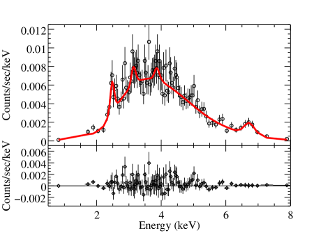
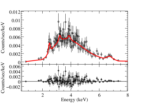
Figure 5: Results of spectral fitting of $5^{\prime\prime}$ region - upper panel for distant background, lower panel for annulus $6^{\prime\prime}-18^{\prime\prime}$. The total model marked with a solid red line is a sum of Galactic absorption (tbabs), thermal bremsstrahlung and four Gaussian lines for Fe, S, Ar and Ca emission.

4 Hot flow around Sgr A*

Chandra ACIS-I camera spatially resolves close vicinity of the central supermassive black hole and the observations constrain the model of hot plasma around Sgr A*. Previously, Shcherbakov & Baganoff (2010) analyzed 953 ksec Chandra data and they have fitted model of hot plasma interacting with stars up to $5^{\prime\prime}$ from the Sgr A* complex. They have provided density and temperature radial profiles of the hot plasma at the outer radius of the flow to be equal: $T=2$ keV and $n_{\rm e}=60$ cm^-3. More recently, Wang et al. (2013) reported 3 Msec observations of Sgr A*, where they have concluded that RIAF model, when the spectrum is fitted by calculating emissivity from RIAF temperature and density profiles, provides an excellent spectral fit indicating the plasma temperature to be 1 keV. Unfortunately, the authors did not fit surface brightness profile to the data.

In the data extracted by us, the collected counts per pixel square are above 30 in the center and a few at $10^{\prime\prime}$ (Fig. 2 red line). Below we present the fit to the surface brightness profile with the model of the hot Bondi flow. The purpose of our studies is to show to which extend the Bondi flow works. In principle in the very centre star influence can be inefficient as discussed by Shcherbakov & Baganoff (2010). In any of such models or RIAF model with outflow, there exists a stagnation radius, which indicates the border between the matter inflowing or outflowing from the very center. At the stagnation radius the Bondi flow stops to be valid, as we show in the section below.

4.1 Dynamical model of the hot accretion flow

We compute model brightness profile based on a standard spherical accretion flow theory (Bondi 1952). The plasma density, temperature, and velocity radial profiles are obtained by solving the general Bondi equations (the conservation equations given in Shapiro & Teukolsky 1983, equations G.21 and G.22). In particular we solve the following Bernoulli equation:

$$h\sqrt{1-\frac{2}{r}+u^{\rm r}}=h_{\rm s}\sqrt{1-3*cs_{\rm s}^{2}}$$ (1)

where fluid enthalpy is $h=1/(1-cs^{2}/(\gamma_{\rm ad}-1))$, $cs$ is the speed of sound, $u^{\rm r}$ is the fluid velocity, and the right-hand-side is the integration constant, found by taking the $h$ and $cs$ at the sonic radius, denoted with underscore s. The speed of sound at the sonic radius $r_{s}$ is given by $cs_{\rm s}^{2}=1/(2*r_{\rm s}-3)$ (see Eq.G17 in Shapiro & Teukolsky 1983). The adiabatic index is assumed to be $\gamma_{\rm ad}\approx 5/3$. Although we use equations that generalize Bondi equations for the Schwarzschild spacetime, our solutions at large distances from the black hole naturally converge to the classical Bondi solution.

The above Bondi model has two (except $\gamma_{\rm ad}$ which is fixed in our model) free parameters: density $n_{\rm e}^{\rm out}$ and temperature of plasma $T_{\rm e}^{\rm out}$, both at the outer radius $R_{\rm out}\geq 10^{\prime\prime}$. These variables are assumed far away from the black hole, and so they are equivalent to the “infinity” values (i.e. $n_{\rm e}^{\rm out}\equiv n_{\infty}$, $T_{\rm e}^{\rm out}\equiv T_{\infty}$). The mass accretion rate onto the black hole in the Bondi models in the units of g s^-1 is:

$$\dot{M}=4\pi\lambda_{s}\frac{(GM_{\rm BH})^{2}\rho_{\infty}}{c_{\rm s,\infty}^{3}}$$ (2)

where $\lambda_{\rm s}$ is a function of adiabatic index $\gamma_{\rm ad}$ (for our $\gamma_{\rm ad}\approx 5/3$, $\lambda_{\rm s}=0.25$). We integrate the model equations from $R_{\rm out}$ down to the black hole horizon. The list of models explored in this work is given in the Tab. 3.

Table 3: List of spherical accretion model parameters ($n_{e,\infty}$ and $T_{\infty}$) with the corresponding mass accretion rate (Eq.2), the speed of sound at the infinity, and Faraday Rotation measures for assumed radial, coherent, moderate ($\beta=1$) and weak ($\beta=10^{7}$) magnetic fields. Fifth and sixth columns show RM_GC computed towards Galactic Center, while seventh and eight columns represent RM_Pulsar computed towards pulsar PSR J1745-2900, located $3^{\prime\prime}$ away from Sgr A* in the projected distance. For comparison, the measured value of RM${}^{*}_{\rm GC}=5.6\pm 0.7\times 10^{5}$ rad/m² (Marrone et al. 2007), and RM${}^{*}_{\rm Pulsar}=6.696\pm 0.004\times 10^{4}$ rad/m² (Eatough et al. 2013).

$\rho_{\infty}$	$T_{\infty}$	$\dot{M}$	$c_{s,\infty}$	RMGC ($\beta=1$)	RMGC ($\beta=10^{7}$)	RMPulsar ($\beta=1$)	RMPulsar ($\beta=100$)
${\rm[cm^{-3}]}$	[keV]	${\rm[M_{\odot}yr^{-1}]}$	${\rm[cms^{-1}]}$	${\rm[rad/m^{2}]}$	${\rm[rad/m^{2}]}$	${\rm[rad/m^{2}]}$	${\rm[rad/m^{2}]}$
1	1	$4.6\times 10^{-7}$	$3.9\times 10^{7}$	$4.4\times 10^{8}$	$1.4\times 10^{5}$	$4.5\times 10^{2}$	40
1	3.5	$7.1\times 10^{-8}$	$7.4\times 10^{7}$	$2.6\times 10^{7}$	$8.4\times 10^{3}$	$6.6\times 10^{2}$	70
1	4	$5.8\times 10^{-8}$	$7.9\times 10^{7}$	$2.0\times 10^{7}$	$6.2\times 10^{3}$	$7.1\times 10^{2}$	70
1	5	$4.1\times 10^{-8}$	$8.9\times 10^{7}$	$1.2\times 10^{7}$	$3.8\times 10^{3}$	$7.8\times 10^{2}$	80
1	6	$3.1\times 10^{-8}$	$9.7\times 10^{7}$	$7.9\times 10^{6}$	$2.5\times 10^{3}$	$8.4\times 10^{2}$	80
1	8	$2.0\times 10^{-8}$	$1.1\times 10^{8}$	$4.1\times 10^{6}$	$1.3\times 10^{3}$	$9.6\times 10^{2}$	$1.0\times 10^{2}$
1	16	$7.2\times 10^{-9}$	$1.5\times 10^{8}$	$9.0\times 10^{5}$	$3.0\times 10^{2}$	$1.3\times 10^{3}$	$1.3\times 10^{2}$
18.3	3.5	$1.3\times 10^{-6}$	$7.4\times 10^{7}$	$2.1\times 10^{9}$	$6.6\times 10^{5}$	$5.2\times 10^{4}$	$5.2\times 10^{3}$
18.4	3.5	$1.3\times 10^{-6}$	$7.4\times 10^{7}$	$2.1\times 10^{9}$	$6.6\times 10^{5}$	$5.3\times 10^{4}$	$5.3\times 10^{3}$
35	1	$1.6\times 10^{-5}$	$3.9\times 10^{7}$	$9.1\times 10^{10}$	$2.9\times 10^{7}$	$9.3\times 10^{4}$	$9.3\times 10^{3}$
35	3.5	$2.4\times 10^{-6}$	$7.4\times 10^{7}$	$5.5\times 10^{9}$	$1.7\times 10^{6}$	$1.4\times 10^{5}$	$1.4\times 10^{4}$
35	4	$2.0\times 10^{-6}$	$7.9\times 10^{7}$	$4.1\times 10^{9}$	$1.3\times 10^{6}$	$1.5\times 10^{5}$	$1.5\times 10^{4}$
35	5	$1.4\times 10^{-6}$	$8.9\times 10^{7}$	$2.5\times 10^{9}$	$7.8\times 10^{5}$	$1.6\times 10^{5}$	$1.6\times 10^{4}$
35	6	$1.1\times 10^{-6}$	$9.7\times 10^{7}$	$1.6\times 10^{9}$	$5.2\times 10^{5}$	$1.7\times 10^{5}$	$1.7\times 10^{4}$
35	8	$7.2\times 10^{-7}$	$1.1\times 10^{8}$	$8.6\times 10^{8}$	$2.7\times 10^{5}$	$2.0\times 10^{5}$	$2.0\times 10^{4}$
35	16	$2.5\times 10^{-7}$	$1.5\times 10^{8}$	$1.8\times 10^{8}$	$5.8\times 10^{4}$	$2.8\times 10^{5}$	$2.8\times 10^{4}$
60	1	$2.8\times 10^{-5}$	$3.9\times 10^{7}$	$2.0\times 10^{11}$	$6.4\times 10^{7}$	$2.1\times 10^{5}$	$2.1\times 10^{4}$
60	3.5	$4.2\times 10^{-6}$	$7.4\times 10^{7}$	$1.2\times 10^{10}$	$3.9\times 10^{6}$	$3.1\times 10^{5}$	$3.1\times 10^{4}$
60	4	$3.4\times 10^{-6}$	$7.9\times 10^{7}$	$9.1\times 10^{9}$	$2.9\times 10^{6}$	$3.3\times 10^{5}$	$3.3\times 10^{4}$
60	5	$2.5\times 10^{-6}$	$8.9\times 10^{7}$	$5.5\times 10^{9}$	$1.7\times 10^{6}$	$3.6\times 10^{5}$	$3.6\times 10^{4}$
60	6	$1.9\times 10^{-6}$	$9.7\times 10^{7}$	$3.7\times 10^{9}$	$1.2\times 10^{6}$	$3.9\times 10^{5}$	$3.9\times 10^{4}$
60	8	$1.2\times 10^{-6}$	$1.1\times 10^{8}$	$1.9\times 10^{9}$	$6.1\times 10^{5}$	$4.4\times 10^{5}$	$4.5\times 10^{4}$
60	16	$4.6\times 10^{-7}$	$1.5\times 10^{8}$	$4.1\times 10^{8}$	$1.3\times 10^{5}$	$6.2\times 10^{5}$	$6.2\times 10^{4}$

To create synthetic brightness profiles, we first generate images of the inner region of the GC $20^{\prime\prime}\times 20^{\prime\prime}$ using a ray tracing method. Our scheme performs radiation transfer through the three dimensional spherically symmetric accretion flow model and records the radiation flux density at each of the detector pixels. In our modelling, we assume that the X-ray radiation is produced by bremsstrahlung. We solve the radiation transfer equation along many rays, using the following bremsstrahlung emissivity function:

$$\epsilon_{\rm ff,\nu}=6.8\times 10^{-38}\,n_{\rm e}^{2}\,\,T_{\rm e}^{-1/2}\,\exp\left(\frac{-h\nu}{kT}\right).$$ (3)

The plasma absorptivity is also taken into account and it is derived from the Kirchhoff’s law of thermal radiation: $\alpha_{\rm ff,\nu}=\epsilon_{\rm ff,\nu}/B_{\nu}$, where $B_{\nu}$ is the Planck function.

To convert the theoretical flux to counts detected by ACIS-I Chandra CCD, the model fluxes are convolved with the instrument response. The total number of counts detected during the exposure time $T_{\rm exp}$ is:

$$C_{\rm tot}=\int T_{\rm exp}\,F_{\rm\nu}\,A_{\rm eff}(\nu)\,\nu^{-1}\,exp(-abs(\nu)\,N_{\rm H})\,d\nu,$$ (4)

where $\nu$ is a frequency corresponding to energies from 0.5 up to 8 keV. Additionally, we assume that absorption also takes place in the ISM between the outer boundary of accretion model and the detector. Hence, we multiply the flux by additional exponential function, and $N_{\rm H}=10^{23}$ cm^-2 is a typical column density of the ISM. Effective area of the instrument $A_{\rm eff}(\nu)$ and absorption coefficient in the ISM abs$(\nu)$ are energy dependent; we adopt the same dependencies as in Shcherbakov & Baganoff (2010, priv. communication).

The final modelled emissivity profiles are obtained by mapping the square images ($20^{\prime\prime}\times 20^{\prime\prime}$) onto 40 concentric rings (the same rings that were used for extracting the data. The total count rate collected on each ring is divided by that ring area (ring area is given in a units of pixels).

Thus computed profiles have to be convolved with the PSF derived for our particular observation in Sec. 2.3. Examples of convolved models of Bondi hot accretion are shown in Fig. 6 by dotted and short dashed lines for two outer temperatures equal 1 and 3.5 keV respectively. For fitting procedure, we have computed a grid of models with different temperatures and densities ranging in $T_{\rm e}^{\rm out}=1-16$ keV and $n_{\rm e}^{\rm out}=1-60$ cm^-3 (see Tab. 3).

4.2 The best model of the surface brightness profile

We fit the model emissivity profile from the Bondi accretion flow convolved with instrument response and with the PSF to the observed surface brightness profile. In Fig. 3 (lower panel) the residuals of fitting up to $10^{\prime\prime}$ are shown. The fit is not statistically acceptable, showing that the uniform Bondi flow is not a good representation for the hot plasma at distances up to $10^{\prime\prime}$ from Sgr A*. In previous analysis by Shcherbakov & Baganoff (2010) a dynamical model of the hot plasma interacting with stars was fitted to the surface brightness profile up to the $5^{\prime\prime}$ from GC. Additionally, Wang et al. (2013) pointed out that Bondi accretion flow ends at the radius $\sim 3.6\times 10^{5}R_{\rm Schw}$ which is $3.8^{\prime\prime}$ in the case of $M=4.4\times 10^{6}M_{\odot}$ black hole.

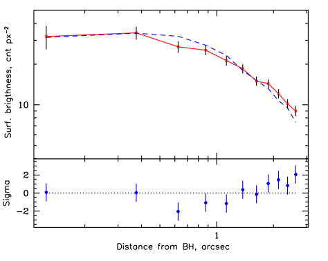
Figure 6: Surface brightness profile up to $3^{\prime\prime}$ away from Sgr A*. Red points represent observed profile, and are connected by continuous line. The best fit model with $T_{\rm e}^{\rm out}=3.5\pm 0.3$ keV and $n_{\rm e}^{\rm out}=18.3\pm 0.1$ cm^-3 is presented by blue short dashed line, and the fit residuals are presented in the lower panel.

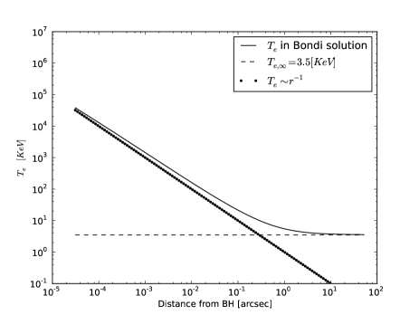
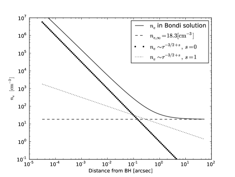
Figure 7: Temperature and density profiles around Sgr A* for our best fitted model $T_{\rm e}^{\rm out}=3.5\pm 0.3$ keV and $n_{\rm e}^{\rm out}=18.3\pm 0.1$ cm^-3, upper and lower panel respectively. The asymptotic values of $T_{\rm e}^{\rm out}$ and $n_{\rm e}^{\rm out}$ are marked as a dashed lines. Additionally, we show the radial dependencies of the temperature and density in RIAF model without (s=0) and with (s=1) an outflow. The normalization of RIAF models is arbitrary.

For this reason, we restricted our modelling to smaller radii and obtained a good fit up to $3^{\prime\prime}$ from Sgr A*. The best theoretical fit profile is shown with a dashed line in the upper panel of Fig. 6, and the parameters of the spherical accretion model are: $n_{\rm e}^{\rm out}=18.3\pm 0.1$ cm^-3 and $T_{\rm e}^{\rm out}=3.5\pm 0.3$ keV. The corresponding integrated mass accretion rate is $\dot{M}=1.3\times 10^{-6}$  M_⊙ yr^-1 . The reduced $\chi^{2}$ of our best fit is 1.19. Residuals are presented in the lower panel of Fig. 6. All data points are within 2 sigma from the model.

From the best fitting model we can estimate profiles of temperature and density of the hot plasma. We present them in Fig. 7 with solid lines. As a result of our fitting we found the values of density and temperature at the distance of $1.5^{\prime\prime}$ to be $n_{\rm e}=29.2$ cm^-3 and $T_{\rm e}=4.8$ keV, respectively. These values are different than those obtained by Shcherbakov & Baganoff (2010) ($n_{\rm e}=130$ cm^-3 and $T_{\rm e}=2$ keV).

The mass accretion rate from our Bondi best fit model is 10-1000 times larger in comparison to the mass accretion rate limits set by the measurements of the Faraday rotation near the central black hole $10^{-9}<\dot{M}<10^{-7}$  M_⊙ yr^-1 (Bower et al. 2005; Marrone et al. 2006, 2007). Nevertheless, the derived mass accretion rate is always model dependent and the direct comparison is meaningless. The above limits computed by Marrone et al. (2006, see Eq. 8 in this paper) strongly depend how the Faraday rotation measure (RM) relates to the accretion flow and magnetic field projected on the line of integration. To avoid any inaccuracies, we present here RM computed from our models according to the formula: RM=$8.1\times 10^{5}\int n_{e}{\rm B}dl$, where electron density $n_{e}$ is in cm^-3, the path length $dl$ is in pc, and the magnetic field ${\rm B}$ - in Gauss (Gardner & Whiteoak 1966), the last defined by standard formula ${\rm B}^{2}=8\pi P_{\rm gas}/\beta$, where $\beta$ is the plasma parameter.

There is no direct constraint on the magnetic field value in Sgr A*, therefore we consider the case of moderate, and very weak magnetic field. We present RM computed towards the GC from all our models in Tab. 3. Fifth column is for $\beta=1$ (magnetic field in equipartition with the gas), while sixth column is for $\beta=10^{7}$. For $\beta=1$, RM_GC for the best fitted model does not agree with measured value RM${}^{*}_{\rm GC}=5.6\pm 0.7\times 10^{5}$ rad/m² (Marrone et al. 2007). But it fully agrees, if we assume that the magnetic field in the radial direction is very weak i.e. $\beta=10^{7}$. We therefore admit, that our best fit model is not well constrained within approximately $100R_{\rm Schw}$ or the magnetic field in radial direction is very weak. When we start the integration of our model from $5\times 10^{-3}$^′′ (which corresponds to the distance of $464\,R_{\rm schw}$), the resulting RM${}_{\rm GC}=6.91\times 10^{5}$ rad/m² with magnetic field being in equipartition. In this case, our result is in quit good agreement with observations, especially that in the paper by Marrone et al. (2006) (Fig. 4) the integration of models was typically done from $300\,R_{\rm schw}$, and than comparred to the data.

For parameter $\beta=10^{7}$, the magnetic field in the center of the flow is ${\rm B}=5\times 10^{-2}$ Gauss, which is not in agreement with recent found that the strength of ${\rm B}$ in GC is around hundred Gauss (Eatough et al. 2013). Nevertheless, this value was given by authors after they have measured RM toward the pulsar PSR J1745-2900 near the GC. Since all model computations are not precise very close to the black hole, we decided to compare the modelled RM towards the above pulsar, located $3^{\prime\prime}$ in the projected distance from the black hole. Such value was reported recently to be equal RM${}^{*}_{\rm Pulsar}=6.696\pm 0.004\times 10^{4}$ rad/m² (Eatough et al. 2013). We project our density profile and magnetic field on the direction towards the pulsar and compute modelled RM_Pulsar in case of $\beta=1$ and $\beta=100$. We present results in Tab. 3, seventh and eight column respectively.

The RM_Pulsar for the best fitted model agrees very well with the observed value for $\beta=1$. For such value of $\beta$ parameter the magnetic field towards Sgr A* is ${\rm B}=157$ Gauss, from our best fitted model. We conclude, that our model density and temperature profiles, and hence mass accretion rate of about $10^{-6}$ M_⊙ yr^-1 around $3^{\prime\prime}$ are consistent with RM measured toward the GC pulsar. It is possible that the mass accretion rate is reduced at distances closer to the black hole. However, these outflows cannot be accounted for in our simple spherically symmetric model that is fitted to spherically averaged brightness profile.

For comparison Fig. 7 also shows the radial profiles of temperature and gas number density from analytical radiativelly inefficient accretion flow (RIAF) models (Shapiro et al. 1976; Rees et al. 1982). In such models the density profile is given by $n\sim r^{(-3/2+s)}$ where $s$ is parameter that if positive then the RIAF launches an outflow. In Fig. 6 lower panel, we plot density profile for $s=0$ (no outflow) and $s=1$, by big and small dots respectively. The density normalization is arbitrary. In RIAF the temperature profile follows $T\sim r^{-\theta}$ where parameter $0<\theta<1$ (the same figure upper panel). Typically in RIAF $\theta=1$ , i.e. temperature has a virial profile (Wang et al. 2013). In Bondi spherical accretion below the sonic point the density profile follows the same radial dependency as in RIAF without the outflow (i.e. s=0), and the temperature is virial. However, the Bondi solutions at large radii naturally connects to constant values, and both, density and temperature profiles deviate from the $n\sim r^{-3/2}$ and $T\sim r^{-1}$ laws, despite of the fact that there is no outflow in this solution.

Our result does not contradict other accretion flow models considered in case of Sgr A*. It shows the position of stagnation radius to be at $3^{\prime\prime}$. Outside this distance, profiles derived by us may not work.

5 Conclusions

In this paper we presented 134 ks Chandra ACIS-I observations of the GC containing the Sgr A* region. After analysing flux images in the continuum (0.5 – 8 keV) and iron line (6.3 – 7.0 keV) bandpasses, we have extracted spectrum of $5^{\prime\prime}$ circular region around Sgr A*. Our spectral model consists of a thermal plasma for the continuum plus Gaussian profiles for the K_α emission of Fe, S, Ar and Ca lines. The continuum is well fitted by a thermal bremsstrahlung emission indicating temperatures for the plasma around Sgr A* in the 2.2 – 2.7 keV range, depending on the choice of background. The corresponding absorbing column densities towards the source are 10.5 – 9.2$\times 10^{22}$ cm^-2, and the corresponding EWs of Fe${}_{K_{\alpha}}$ line are 1.19 – 0.91 keV. Our spectral fitting indicates lower temperature by about 0.5 keV than this obtained by Wang et al. (2013) with the same model. Nevertheless, the strength of iron line consistent with that reported by Wang et al. (2013) at the $1\sigma$ confidence level.

Furthermore, we studied the brightness profile of the hot plasma in the vicinity of the Sgr A* black hole. We found that the classical Bondi accretion can reproduce observed brightness profile up to $3^{\prime\prime}$. This result implies strong constrains on the position of stagnation point always considered to be present in the complicated flow around Sgr A*. The best fit model for surface brightness profile requires that the hot plasma outside the flow to have temperature $T_{\rm e}=3.5\pm 0.3$ keV and density $n_{\rm e}=18.3\pm 0.1$ cm^-3.

Sgr A* has been recently resolved down to $1.5^{\prime\prime}$ and studied by Wang et al. (2013). They have reported an X-ray image of the source based on a 3 Msec Chandra observation. The best fitted model was RIAF (radiatively inefficient accretion flow), but they did not show any resulting temperature and density profiles. Only a general description for the temperature dependence on the distance was given as: $T\propto r^{-\theta}$ where $\theta\gtrsim 0.6$. Additionally, they concluded from the weak line of H-like iron Fe XXVI, that the amount of gas at temperatures $\sim 9$ keV is very small. Our temperature profile predicts the temperature of 9 keV at the distance $0.4^{\prime\prime}$ from the black hole. Such plasma would have number density equal to 70 cm^-3. Both temperature profiles, RIAF and Bondi, agree up to $0.1^{\prime\prime}$, as it is seen in Fig. 7. But Bondi flow fitted by us predicts higher density by one order of magnitude.

All models show different temperatures at the outer parts of the flow $T_{\rm e}$ = 1, 2, and 3.5 keV respectively in the RIAF model (Wang et al. 2013), hot plasma fed by stars (Shcherbakov & Baganoff 2010), and the only Bondi flow reported in this paper. Additionally, spectral fitting done by us and Wang et al. (2013) indicates slightly different temperatures (2.7 and 3.5 respectively). Those results show a big complexity of matter structure around Sgr A*, and additional indications should be taken into account when studying hot plasma in this region. For instance Wang et al. (2013) also found the He-like Fe K_α line. Therefore, we argue, that up to $3^{\prime\prime}$ Bondi flow works, but further away hot matter may be in the form of two-phase medium. We speculate that the Fe K_α line emission at $6.69$ keV can be attributed to the reflection from clouds of the warm gas. This illuminated radiation originates from the very innermost nucleus and depending on the luminosity state of Sgr A*, can provide strong clumpiness and trigger formation of such hot clouds, as proposed by Różańska et al. (2014). However, it is critically important to confirm that the Bondi model fitted here does not overpredict the strength of the FeXXVI line. Wang et al. (2013) concluded that due to the weakness of FeXXVI line, there must be a little gas at temperatures larger than 9 keV. In our Bondi model the gas temperature reaches 9 keV at $0.4"$ (compared to $\leavevmode\nobreak\ 0.1"$ in the RIAF model). If the strength of this line computed from our best fitted model of Bondi flow disagrees with the observed one, this may rule out of our model despite its agreement with the surface brightness profile. To fully check our predictions we plan to construct the model of thermal plasma. Also, better spectrum will be needed for this kind of analysis.

The mass accretion rate from our Bondi best fit model is $1.3\times 10^{-6}$  M_⊙ yr^-1. This is out of the range of accretion rates predicted from measurements of the Faraday rotation (RM) (Marrone et al. 2007). Nevertheless, we point out that the derived mass accretion rate limits are always model dependent. Especially we can modify them by changing the structure and strength of a magnetic field. For our best fitted model the computed RM_GC agrees with observed one toward Galactic Center with assumption of very weak radial magnetic field. Moreover, RM_Pulsar computed from the best fit model towards the pulsar PSR J1745-2900 located at $3^{\prime\prime}$ projected distance from GC is in very good agreement with observations assuming moderate magnetic field, $\beta=1$. This result clearly shows that any limitation on accretion rate from Faraday rotation strongly depends on the model and orientation of magnetic field. We admit that the best way to compare the accretion model to Faraday rotation measure is not by comparing accretion rates, but by self consistent calculations of RM from the model.

Profiles of temperature and density resulting from our fitting put constraints on the physical conditions in the vicinity of the GC. It may provide information on the value of the gas pressure of the hot plasma. Together with radiation pressure taken from observed luminosity states of Sgr A* we can estimate the size of the thermal instability and eventual cloud formation in this region (Różańska et al. 2014). Such multi-phase complex structure is observed in our GC (for review, see Cox 2005). This structure is important from the point of view of feeding the central black hole as well as the possibility of an accompanying outflow.

To study any possible outflow related tot he Sgr A* accretion, we should search for spatially resolved regions of the hot plasma farther away from the Sgr A* region, where the line emission is prominent. For example, strong iron K_α line emission detected in our observations occurs in the Sgr A East region. The origin of this emission is strongly affected by SNR, and more advance spectral model should be used to describe the emerging spectra. We address these studies in the forthcoming paper.