Non–equilibrium Bethe-Salpeter equation for transient photo–absorption spectroscopy

Abstract

In this work we propose an accurate first-principle approach to calculate the transient photo–absorption spectrum measured in Pump& Probe experiments. We formulate a condition of adiabaticity and thoroughly analyze the simplifications brought about by the fulfillment of this condition in the non–equilibrium Green’s function (NEGF) framework. Starting from the Kadanoff-Baym equations we derive a non–equilibrium Bethe–Salpeter equation (BSE) for the response function that can be implemented in most of the already existing ab–initio codes. In addition, the adiabatic approximation is benchmarked against full NEGF simulations in simple model hamiltonians, even under extreme, nonadiabatic conditions where it is expected to fail. We find that the non–equilibrium BSE is very robust and captures important spectral features in a wide range of experimental configurations.

I Introduction

The impressive progresses in ultrafast and ultrastrong laser-pulse technology has paved the way to the modern non–equilibrium (NEQ) attosecond spectroscopies.bgk.2009 ; spsk.2012 ; ghlsllk.2013 ; kc.2014 ; science.2014 Unlike conventional spectroscopies, the sample is driven away from equilibrium by a strong laser pulse (the pump) before the photo–absorption of a weaker (perturbative) probe field is measured. Photo–absorption pump-and-probe (P&p) spectroscopy experiments are carried out using pump pulses with frequency in the infrared-ultraviolet range and ultrashort probe pulses (down to a few hundreds of attoseconds). By varying the delay between the pump and probe pulses one can monitor the excited-state dynamics in a wide energy range.

For samples of linear dimension (in the case of extended systems this is the dimension of the primitive cell) smaller than the wave–length of the incident light, the measured signal can be calculated theoretically from the NEQ density response function bm.1997 ; wssd ; sypl.2011 ; mpb.2012 ; blm.2012 ; dgc.2013 ; PS.2015 $\chi$ (dipole approximation) or, equivalently, from equilibrium dipole correlators of order larger than two. Shen-book ; kbs.1988 ; ym.1990 ; pm.1992 ; Mukamel-book ; yzc.1997 In the present manuscript we follow the first path.

At equilibrium $\chi(\omega)$ can be used to construct the dipole–dipole correlation function $\alpha\left(\omega\right)$ in isolated system, or the dielectric function $\epsilon\left(\omega\right)$ in extended systems. For correlated systems the calculation of $\chi$ is, in general, a difficult task and one has to resort to approximations. The most suitable many–body scheme to implement depends on the sample. For atomic or small molecular samples the Configuration Interaction (CI) scheme consists in expanding the many–body state in Slater determinants to obtain eigenstates and eigenvalues. Subsequently the oscillator strengths are computed and used to construct $\chi$ from a Lehmann representation. For molecules with tens or more nuclei as well as for crystals the number of CI configurations is too large for present-day computational capabilities and alternative (statistical in nature) approaches are required. One such approach is many–body perturbation theory (MBPT). In MBPT the two–particle electron–hole propagator $L$ satisfies a diagrammatic equation known as the Bethe–Salpeter Equation (BSE) and $\chi$ is constructed from a space-time contraction of the arguments of $L$. strinati_review ; svl-book The BSE has been successfully applied to study photo–absorption spectroscopy of systems ranging from small molecules to bulk metals and insulators. In this context the BSE is solved at the GW level with a statically screened interaction.Strinati ; strinati_review ; orr.2002 ; ardo.1998 ; bsb.1998 ; rl.1998 ; pphs.2011 .

Another convenient alternative to CI (and MBPT) is the Linear Response (LR) Time–Dependent Density–Functional Theory (TDDFT). pgg.1996 ; Casida1 Although TDDFT is in principle exact, rg.1984 ; Ullrich the available functionals for actual calculations are based on the Adiabatic Local Density Approximation (ALDA).rozzi-nature ; miguel ; degiovannini It is well known that ALDA functionals fail in capturing double-excitations,mzcb.2004 ; kk.2008 charge transfer excitationsngb.2006 ; m.2005 ; mt.2006 or the Coulomb blockade phenomenonsk.2011 ; ks.2013 in equilibrium systems. For extended systems ALDA performs poorly in the description of the response function as it misses the long–range electron–hole interaction needed to describe excitons.orr.2002 ; roro.2002 Therefore, the applicability of LR–TDDFT is at present restricted to weakly correlated systems with a spectrum dominated by single particle-hole excitations.

Similarly to the equilibrium case the P&p photo–absorption spectrum is described by the NEQ response function $\chi(t,t^{\prime})$. In this work we identify a set of constraints between characteristic times that allows us to rewrite $\chi(t,t^{\prime})$ as a function of the delay $\tau$ between the pump and probe pulses and of the time difference $t-t^{\prime}$, i.e., $\chi(t,t^{\prime})=\chi^{\tau}(t-t^{\prime})$. Henceforth we will refer to this approximation as the adiabatic approximation. The mathematical rigorous definition of the adiabatic approximation as well as its testing in a P&p set-up is the central objective of the present manuscript.

The adiabatic response function can be computed at different levels of accuracy depending on the theoretical scheme used. In the CI approach the time–dependent expansion coefficients are used to calculate the time–dependent product of oscillator strengths and subsequently these products are inserted into a Lehmann–like representation of the NEQ adiabatic $\chi^{\tau}(\omega)$ to yield a P&p spectrum with a time–dependent modulation of the peak intensity.rs.2009 ; nature.2010 ; sypl.2011 ; blm.2012 Within MBPT, instead, we show that the equation of motion for $\chi^{\tau}(t-t^{\prime})$ can be rewritten as a BSE. The main difference with the equilibrium BSE is that the equilibrium single–particle density matrix is replaced by its time–dependent value as, for instance, obtained from the solution of a Boltzmann–like equation. hj-book The NEQ adiabatic $\chi^{\tau}(\omega)$ could also be computed within LR–TDDFT. However, it is reasonable to expect that the performance of ALDA functionals does not improve in NEQ situations.

The structure of the paper is as follows. Section II presents a brief self–contained introduction to the link between the macroscopic observable and the microscopic theory. We discuss both the real–time (Section II.1) and the response function (Section II.2) representations. Here we also identify a set of characteristic times in terms of which the condition of adiabaticity is formulated. The MBPT approach to $\chi$ is developed in Section III where we introduce the non–equilibrium Green’s functions (NEGF).svl-book ; hj-book ; vLDSAvB.2006 ; d.1984 ; bb.2013 ; kb-book The NEGF approach is computationally more expensive than TDDFT but it has the advantage of including dynamical correlations in a nonperturbative diagrammatic fashion. To reduce the numerical cost we implement, in Section III.1, NEGF within the Generalized Kadanoff–Baym Ansatz hj-book ; lsv.1986 (GKBA) and then derive the linear response equations in Section III.2. Except for the GKBA no other approximations are made at this stage. The complexity of the problem is further reduced in Section IV. Here we exploit the adiabatic approximation and obtain the central result of this work, namely a NEQ–BSE. We examine differences and analogies with the more standard equilibrium BSE and discuss the possibility of converting the NEQ–BSE into a Dyson-like equation in Section IV.1. Finally, in Section V we illustrate the theory in a model system by benchmarking the performance of the NEQ–BSE against full NEGF calculations. A summary of the paper and concluding remarks are drawn in Section VI.

II The transient photo–absorption spectrum

In this Section we relate the macroscopic quantity measured in a P&p experiment to microscopic quantum-mechanical properties of the probed sample. This link establishes a connection between the experimental signal and the solution of the complex quantum kinetic equation for the one–particle density–matrix.

II.1 A real time approach

In a P&p experiment the transient photo–absorption spectrum of a system driven out of equilibrium by a pump field is measured. The theoretical description of the driven system is achieved by evolving the many-body state in the simultaneous presence of the pump field and of a weak probe field. Let ${\mathbf{E}}$ and ${\mathbf{e}}$ be the electric pump and probe field respectively. We define the different terms constituting the many–body Hamiltonian $\hat{H}(t)$ according to

$$\hat{H}^{0}=\hat{T}+\hat{V}_{N},$$ (1a)

$$\hat{H}^{\rm eq}=\hat{H}^{0}+\hat{V}_{ee},$$ (1b)

$$\hat{H}^{\rm neq}(t)=\hat{H}^{\rm eq}+{\mathbf{E}}(t)\cdot\hat{{\mathbf{d}}},$$ (1c)

$$\hat{H}(t)=\hat{H}^{\rm neq}(t)+{\mathbf{e}}(t)\cdot\hat{{\mathbf{d}}}.$$ (1d)

Here $\hat{T}$ is the kinetic energy operator, ${\hat{V}_{N}}$ the external static potential of the nuclei and ${\hat{V}_{ee}}$ the electron–electron interaction. Therefore $\hat{H}^{\rm eq}$ is the Hamiltonian of the unperturbed system. The inclusion of other interactions, e.g., the electron-phonon interaction, does not modify the derivation and the results of the present section. The terms ${{\mathbf{E}}(t)\cdot\hat{{\mathbf{d}}}}$ and ${{\mathbf{e}}(t)\cdot\hat{{\mathbf{d}}}}$ describe the coupling of the electrons with the pump and probe fields in the dipole approximation, $\hat{{\mathbf{d}}}$ being the dipole operator (see below for its mathematical definition). For simplicity, we consider linearly polarized pump and probe fields:

$${\mathbf{E}}(t)={\bm{\eta}}_{P}E(t),$$ (2a)

$${\mathbf{e}}(t)={\bm{\eta}}_{p}e(t),$$ (2b)

with ${\bm{\eta}}_{P}$ and ${\bm{\eta}}_{p}$ the polarization vectors. The generalization to other kind of polarizations is straightforward.

We work in the second quantization formalism and introduce a suitable single–particle basis with orthonormal wave–functions $\{\varphi_{i}\left({\mathbf{r}}\right)\}$. Then the creation and annihilation field-operator $\hat{\psi}^{{\dagger}}\left({\mathbf{r}}\right)$ and $\hat{\psi}\left({\mathbf{r}}\right)$ for a particle at position ${\mathbf{r}}$ in space are expanded according to $\hat{\psi}\left({\mathbf{r}}\right)=\sum_{i}\varphi_{i}\left({\mathbf{r}}\right)\hat{c}_{i}$. The one–particle density–matrix operator takes the form

$$\hat{\rho}({\mathbf{r}},{\mathbf{r}}^{\prime})=\hat{\psi}^{{\dagger}}({\mathbf{r}})\hat{\psi}({\mathbf{r}}^{\prime})=\sum_{ij}\varphi^{*}_{i}({\mathbf{r}})\varphi_{j}({\mathbf{r}}^{\prime})\hat{\rho}_{ji},$$ (3)

with $\hat{\rho}_{ji}=\hat{c}^{\dagger}_{i}\hat{c}_{j}$. Similarly, the dipole operator projected along the probe field in the $\{\varphi_{i}\left({\mathbf{r}}\right)\}$ basis reads

$$\hat{d}={\bm{\eta}}_{p}\cdot{\hat{{\mathbf{d}}}\equiv\int d{\mathbf{r}}\;({\bm{\eta}}_{p}\cdot{\bf r})\hat{\rho}({\mathbf{r}},{\mathbf{r}})}=d_{ij}\hat{\rho}_{ji},$$ (4)

with $d_{ij}=\int d{\mathbf{r}}\,\varphi^{*}_{i}({\mathbf{r}})({\bm{\eta}}_{p}\cdot{\bf r})\varphi_{j}({\mathbf{r}})$ the dipole matrix elements. In Eq. (4) and in the remainder of the paper we use the Einstein convention that repeated indices are summed over. The time–dependent expectation value of the dipole operator is given by

$$d\left(t\right)=\langle\Psi(t)|\hat{d}|\Psi(t)\rangle=d_{ij}\langle\Psi(t)|\hat{\rho}_{ji}|\Psi(t)\rangle,$$ (5)

where $|\Psi(t)\rangle$ is the state of the system at time $t$.

Without any loss of generality we assume that the switch-on time of the pump and probe fields is larger than zero; hence the system is in the ground state $|\Psi_{g}\rangle$ at time $t=0$. Let $\hat{\mbox{$\mathcal{U}$}}_{H}(t)$ be the unitary evolution operator corresponding to a system with dynamics $\hat{H}$

$$\hat{\mbox{$\mathcal{U}$}}_{H}(t)\equiv Te^{-i\int_{0}^{t}d\bar{t}\;[\hat{H}(\bar{t})]},\quad t>0.$$ (6)

The time-dependent matrix elements of the one–particle density matrix in the presence of both the pump and probe fields are therefore given by

$$\rho_{ji}(t)\equiv\langle\Psi(t)|\hat{\rho}_{ji}|\Psi(t)\rangle=\langle\Psi_{g}|\,\hat{\mbox{$\mathcal{U}$}}^{{\dagger}}_{H}(t)\hat{\rho}_{ji}\,\hat{\mbox{$\mathcal{U}$}}_{H}(t)|\Psi_{g}\rangle.$$ (7)

Replacing $\hat{H}$ with $\hat{H}^{\rm neq}$ in Eq. (6) we have the evolution operator in the presence of the pump only, ${\hat{\mbox{$\mathcal{U}$}}_{H^{\rm neq}}(t)}$. To simplify the notation we put a tilde on time-dependent expectation values obtained with a probe–free propagation. Thus

$$\tilde{\rho}_{ji}(t)=\langle\Psi_{g}|\,\hat{\mbox{$\mathcal{U}$}}^{{\dagger}}_{H^{\rm neq}}(t)\hat{\rho}_{ji}\,\hat{\mbox{$\mathcal{U}$}}_{H^{\rm neq}}(t)|\Psi_{g}\rangle,$$ (8)

and hence $\tilde{d}(t)=d_{ij}\tilde{\rho}_{ji}(t)$.

For optically thin samples footnote_thin the transmitted probe field ${\mathbf{e}}^{\prime}(t)={\bm{\eta}}_{p}e^{\prime}(t)$ is related to the probe–induced variation $\delta{\bf d}\left(t\right)\equiv{\mathbf{d}}(t)-\tilde{{\mathbf{d}}}(t)$ of the dipole moment byPS.2015

$${\mathbf{e}}^{\prime}(t)={\mathbf{e}}(t)+\frac{2\pi}{Sc}\frac{d}{dt}\left[\delta{\bf d}\left(t\right)\right],$$ (9)

where $S$ is the cross section of the sample (assumed to be smaller than the cross section of the laser beam).

The transmitted probe field is typically split in two halves and then merged back by a spectrometer, thus generating an electric field $\frac{1}{2}[{\mathbf{e}}^{\prime}(t)+{\mathbf{e}}^{\prime}(t-\delta)]$ with a tunable delay $\delta\geq 0$. In a P&p experiment the integrated intensity of this field, i.e., the total absorbed energy per unit area, is measured as a function of $\delta$:

$$I^{\prime}(\delta)=\frac{c}{4\pi}\int_{-\infty}^{\infty}dt\left|\frac{{\mathbf{e}}^{\prime}(t)+{\mathbf{e}}^{\prime}(t-\delta)}{2}\right|^{2}.$$ (10)

The resulting function $I^{\prime}(\delta)$ is then cosine-transformed

$$\mathfrak{I}^{\prime}(\omega)=\int_{0}^{\infty}d\delta\;I^{\prime}(\delta)\cos(\omega\delta),$$ (11)

to gain information about the absorption energies of the system. Although the probe pulse has a finite duration the time integral in Eq. (10) goes from minus to plus infinity since the cosine transform requires $I^{\prime}(\delta)$ for all delays $\delta\geq 0$.

Performing an analogous spectral decomposition of ${\mathbf{e}}(t)$ we get the intensity $\mathfrak{I}(\omega)$ of the incident probe field. The photo–absorption spectrum $\mathfrak{S}(\omega)$ is therefore given by the difference

$$\frac{\mathfrak{S}(\omega)}{S}=\mathfrak{I}(\omega)-\mathfrak{I}^{\prime}(\omega).$$ (12)

Using Eq. (9) it is straightforward to show thatPS.2015

$$\mathfrak{S}(\omega)=-2\omega\,{\rm Im}\left[e\left(\omega\right)\delta d\left(\omega\right)\right]-\frac{2\pi}{Sc}\left|\omega\delta d(\omega)\right|^{2},$$ (13)

where $e\left(\omega\right)$ and $\delta d\left(\omega\right)$ are the Fourier transform of the time-dependent probe field $e(t)$ and probe–induced dipole moment $\delta d(t)$ respectively. This relation expresses the aforementioned link between the macroscopic intensity of the transmitted probe field measured in a P&p experiment and the microscopic dipole moment.

In photo–absorption experiments of equilibrium systems (no pump) the induced electric field [second term in the r.h.s. of Eq. (9)] is typically much smaller than the incident probe, and the quadratic term in the dipole moment appearing in $\mathfrak{S}(\omega)$ can be safely discarded. Moreover, $\delta d(\omega)=\alpha(\omega)e(\omega)$ with $\alpha(\omega)\equiv d_{ij}\chi_{\begin{subarray}{c}ji\\ kl\end{subarray}}(\omega)d_{lk}$ having the property that ${\rm Im}[\alpha(\omega)]\lessgtr 0$ for $\omega\gtrless 0$ (see next section), and therefore the ratio $\mathfrak{S}(\omega)/|e(\omega)|^{2}$ is positive and independent of the shape of the probe. On the contrary, the photo–absorption spectrum of a pump driven system is not an intrinsic property of the sample since $\delta d(\omega)$, although still linear in $e$, depends on $e(\omega^{\prime})$ at all possible frequencies $\omega^{\prime}$. Translating this statement from frequencies to times, the spectrum depends on the shape of the probe and on the NEQ state of the system at the time the probe pulse enters the sample (hence on the delay between the pump and probe pulses). Furthermore, there might be frequencies for which the spectrum $\mathfrak{S}(\omega)$ is negative due to a dominance of the stimulated emission over absorption.

For a fixed shape of the pump and probe pulse the main interest in P&p experiments is to study the evolution of the spectrum as the delay $\tau$ between the two pulses is varied. Assuming that the quadratic term in $\delta d$, see Eq. (13), is small and taking into account that $\delta d(\omega)=d_{ij}[\rho_{ji}(\omega)-\tilde{\rho}_{ji}(\omega)]$, the resulting spectrum reads

$$\mathfrak{S}^{\tau}(\omega)=-2\omega\,{\rm Im}\left[e^{\ast}(\omega)d_{ij}\delta\rho_{ji}(\omega)\right],$$ (14)

where we define $\delta\rho=\rho-\tilde{\rho}$. In Eq. (14) we explicitly added to $\mathfrak{S}$ a dependence on $\tau$ since the probe field as well as the time-dependent density matrix depends on the pump–probe delay. This dependence is, in general, rather complex and difficult to interpret. As we shall see, the calculation of the spectrum as well as its physical interpretation are greatly simplified if the adiabatic approximation is made.

II.2 A response–function representation: the adiabatic condition

Equation (14) can be rewritten in a different way using linear response theory out of equilibrium. Let us introduce the (retarded) NEQ response function

$$\chi_{\begin{subarray}{c}ji\\ lk\end{subarray}}\left(t,t^{\prime}\right)=-i\theta\left(t-t^{\prime}\right)\\ \times\langle\Psi_{g}|\left[\hat{c}^{\dagger}_{iH}\left(t\right)\hat{c}_{jH}\left(t\right),\hat{c}^{\dagger}_{kH}\left(t^{\prime}\right)\hat{c}_{lH}\left(t^{\prime}\right)\right]|\Psi_{g}\rangle,$$ (15)

where $\hat{c}_{iH}(t)\equiv\hat{\mbox{$\mathcal{U}$}}^{{\dagger}}_{H^{\rm neq}}(t)\hat{c}_{i}\,\hat{\mbox{$\mathcal{U}$}}_{H^{\rm neq}}(t)$ are fermion operators in the Heisenberg picture with respect to the probe–free Hamiltonian $\hat{H}^{\rm neq}$. To first order in ${\mathbf{e}}$ the probe–induced variation of the dipole moment reads

$$\delta d\left(t\right) = d_{ij}\int dt^{\prime}\chi_{\begin{subarray}{c}ji\\ lk\end{subarray}}\left(t,t^{\prime}\right)d_{kl}\,e(t^{\prime})$$ (16)

$$= \int dt^{\prime}\left[d\circ\chi\left(t,t^{\prime}\right)\circ d\right]e(t^{\prime}).$$

In Eq. (16) we introduced a short–hand notation for the contraction of tensors of different rank. Below we define the four types of contractions, which include the one in Eq. (16), that we use in the manuscript:

$$(M\circ V)_{pq}\equiv M_{\begin{subarray}{c}pq\\ mn\end{subarray}}V_{nm},$$ (17a)

$$(T\circ M\circ V)\equiv T_{pq}M_{\begin{subarray}{c}qp\\ mn\end{subarray}}V_{nm},$$ (17b)

$$(M\circ N)_{\begin{subarray}{c}mn\\ rs\end{subarray}}\equiv M_{\begin{subarray}{c}mn\\ pq\end{subarray}}N_{\begin{subarray}{c}qp\\ rs\end{subarray}},$$ (17c)

$$[N,V]_{\begin{subarray}{c}mn\\ pq\end{subarray}}=-[V,N]_{\begin{subarray}{c}mn\\ pq\end{subarray}}\equiv N_{\begin{subarray}{c}mi\\ pq\end{subarray}}V_{in}-V_{mi}N_{\begin{subarray}{c}in\\ pq\end{subarray}}.$$ (17d)

The rank of the tensors will be clear from the context. Notice that Eq. (17d) has the same structure of a commutator since the lower indices are fixed. Taking into account Eq. (14) we clearly see from Equation (16) the relation between the P&p spectrum and the NEQ response function; we can also appreciate the complex time dependence introduced by the pump field. In fact, in equilibrium (no pump) the response function reduces to a function of $\left(t-t^{\prime}\right)$ due to the invariance under time-translations. Using this invariance, the linear response relation Eq. (16) in Fourier space reads $\delta d(\omega)=\alpha(\omega)e(\omega)$ with $\alpha=\left(d\circ\chi\circ d\right)$, and the ratio $\mathfrak{S}(\omega)/|e(\omega)|^{2}$ becomes independent of the probe. As already discussed in the introduction the equilibrium response function can be calculated by solving the BSE.

In the time domain the equation for the electron-hole propagator $L$ ($\chi$ follows from a space-time contraction of $L$) is valid out-of-equilibrium too svl-book but its numerical solution is essentially impossible for present-days computational capabilities. The problem is therefore to find a simple but still accurate approach to calculate the NEQ $\chi$ within MBPT. For this purpose we will extend the equilibrium BSE to NEQ situations relevant to P&p experiments and provide a sound interpretation of the two–time dependence. In the following we refer to this equation as the NEQ–BSE.

We begin the discussion by introducing two fundamental characteristic times that support the adiabatic approximation: the key idea is that a NEQ–BSE is meaningful whenever the system is substantially frozen in a NEQ configuration during the measurement process. The characteristic times are

• the time scale $T_{P}$ of the electron dynamics induced by the pump. If $\Delta t\ll T_{P}$, then $\tilde{\rho}\left(t+\Delta t\right)\approx\tilde{\rho}\left(t\right)$.

• the life–time $\tau_{p}$ of the dressed probe pulse, which is the duration of the measurement process too.

We can formulate the condition of applicability of the adiabatic approximation as

$$T_{P}\gg\tau_{p}.$$ (18)

Equation (18) expresses the physical condition that the probe–free $\tilde{\rho}(t)$ has to vary on a time scale ($T_{P}$) much longer than the duration ($\tau_{p}$) of the dressed probe. Of course for $\tau_{p}$ to be smaller than typical electronic time scales there should exist decay channels faster than the radiative decay. This is the case of solid slabs as well as of thick atomic or molecular gases. The following analysis applies to these class of systems.

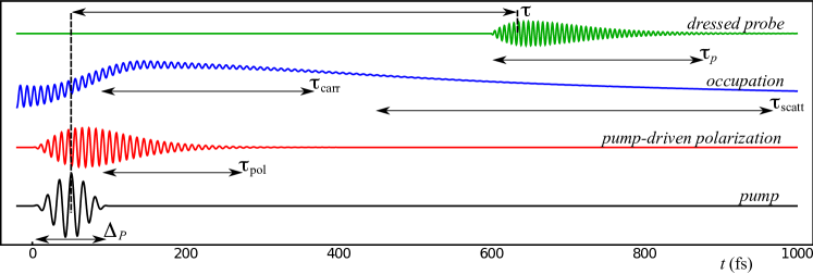
Figure 1: Illustration of the characteristic times described in the main text: $T_{P}$ is the time scale of the electron dynamics induced by the pump, $\tau_{\rm pol}$ the dephasing time of the pump-induced polarization, $\tau_{\rm carr}$ the stabilization time of the occupations, $\tau_{\rm scatt}$ the time to relax back to the equilibrium state and $\tau_{p}$ the life–time of the dressed probe field. We also display the delay $\tau$ between pump and probe.

We identify two different situations where the condition in Eq. (18) is fulfilled. 1) If the pump itself varies on a time scale $T_{P}\gg\tau_{p}$ then Eq. (18) is always fulfilled since the pump-induced dynamics cannot be faster than $T_{P}$. In this case the adiabatic approximation, and hence the NEQ–BSE, can be used to describe the transient spectrum for any delay $\tau$ between the pump and probe fields. 2) In general, however, the pump is a pulse of duration $\Delta_{P}$, see Fig. 1, no longer than a few hundreds of femtoseconds capable of inducing arbitrary fast processes. During the action of the pump the level occupations change and the system polarizes. Shortly after $\Delta_{P}$ we have a transient period characterized by a dephasing-driven drop of the pump-induced polarization, we denote by $\tau_{\rm pol}$ the polarization life–time in this nonequilibrium situation, and by a stabilization of the level occupations at some nonequilibrium value, we denote by $\tau_{\rm carr}$ the characteristic time for the occupations to stabilize, see again Fig. 1. Thus, after a time $\tau_{\rm max}={\rm max}(\tau_{\rm pol},\tau_{\rm carr})$, typically $\tau_{\rm pol}<\tau_{\rm carr}$, we may say that the system is in a quasi–stationary state with carriers in some excited levels. In this quasi–stationary regime the time to relax back to the ground state is dictated by scattering processes (electron–electron, electron–phonon and electron–photon) and can be of the order of picoseconds. If we denote by $\tau_{\rm scatt}$ this relaxation time-scale then we have $T_{P}=\tau_{\rm scatt}$. Suppose now to probe the system in this quasi–stationary state with a pulse $e(t)$ of duration $\Delta_{p}$. The probe induces a polarization $\delta d(t)$ which dresses the bare $e(t)$ and, in general, has a finite life–time $\tilde{\tau}_{p}$. Hence the duration of the dressed probe field, which coincides with the duration of the measurement process, is $\tau_{p}=\Delta_{p}+\tilde{\tau}_{p}$. In this regime the condition in Eq. (18) is fulfilled provided that $\tau_{p}$ is shorter than the relaxation time $\tau_{\rm scatt}$. This is often the case as $\tau_{p}$ is typically in the femtosecond range.

In Fig. 1 we represent the dressed probe field with oscillations of frequency $\omega_{p}$. Although the characteristic frequency $\omega_{p}$ can be any, it is clear that it is only for

$$\tau_{p}\gg\frac{2\pi}{\omega_{p}}$$ (19)

that the Fourier transform of the probe–induced dipole has a well defined structure in $\omega_{p}$. This implies that the life–time $\tau_{p}$ also sets a lower limit to the frequency resolution of a transient spectroscopy experiment.

When the inequality of Eq.  (18) is satisfied the probe sees a NEQ frozen system. If we take $t=0$ as the time at which the pump is on then the probe acts at $t=\tau$ and for times $(t,t^{\prime})\in[\tau-\tau_{p},\tau+\tau_{p}]$ the response function

$$\chi(t,t^{\prime})\approx\chi^{\tau}(t-t^{\prime})$$ (20)

depends only on $(t-t^{\prime})$ to a large extent. We will provide a more precise definition of $\chi^{\tau}(t-t^{\prime})$ in the next section. For the time being we observe that whenever we can make the adiabatic approximation of Eq. (20) the transient photoabsorption spectrum of Eq. (14) can be written as

$$\mathfrak{S}^{\tau}(\omega)=-2\omega\,|e(\omega)|^{2}\,{\rm Im}\left[d\circ\chi^{\tau}(\omega)\circ d\right].$$ (21)

Consequently the ratio $\mathfrak{S}^{\tau}(\omega)/|e(\omega)|^{2}$ becomes independent of the probe and can be interpreted as an intrinsic property of the nonequilibrium system.

As a very general remark we notice that when the system is probed after the pump (no overlap between the pulses) the probe–induced dipole moment oscillates at frequencies $\Omega_{\alpha\beta}=E_{\alpha}-E_{\beta}$, where $E_{\alpha},E_{\beta}$ are eigen–energies of $\hat{H}^{\rm eq}$, see Eqs. (15) and (16).PS.2015 ; FLSM.2015 Furthermore, the amplitude of the oscillations depends on the delay $\tau$.PS.2015 Therefore P&p spectra are richer than equilibrium spectra where the probe–induced dipole moment can oscillate only at frequencies $\Omega_{\beta}=E_{g}-E_{\beta}$, with $E_{g}$ the ground state energy, with constant amplitudes. The extra transitions are usually referred to as photo–induced absorption and stimulated emission.

To summarize, Eqs. (14) and (21) represent two different ways of calculating the transient photo–absorption spectrum. We could either perform a time propagation with both the pump and the probe, a second time propagation with only the pump and then extract the probe–induced dipole moment $\delta d$ or we can evaluate the response function $\chi^{\tau}$ from a NEQ–BSE. The latter approach is developed in the next section.

III A non–equilibrium Green’s function approach to transient absorption

In the previous section we have introduced the theoretical description of transient absorption experiments with two possible approaches. The first, which is exact, based on Eq. (14) and the second, which uses the adiabatic approximation, based on Eq. (21). However, these equations assume that it is ideally possible to compute the exact time-dependent density matrix or the exact adiabatic response function. This is not doable in practice and one has to resort to approximations. In the following we show how to use NEGF theory to obtain a MBPT equation for $\delta d\left(t\right)$. In the next Section we use this result to generate an equation for the NEQ response function $\chi(t,t^{\prime})$, and subsequently make the adiabatic approximation to derive the NEQ–BSE for $\chi^{\tau}(t-t^{\prime})$.

In the MBPT approach the description in terms of the many–body hamiltonian containing the electron–electron interaction is replaced by a description in terms of the one particle hamiltonian and the many–body self–energy. We thus define:

$$h^{0}=\left[-\frac{\nabla^{2}}{2}+V_{N}({\mathbf{r}})\right],$$ (22a)

$$h^{\rm eq}=h^{0}+\Sigma^{0},$$ (22b)

$$\tilde{h}^{t}(t)=h^{\rm eq}+\Delta\tilde{\Sigma}_{s}^{t}+{\mathbf{E}}(t)\cdot{\mathbf{d}},$$ (22c)

$$h^{t}(t)=\tilde{h}^{t}(t)+\delta\Sigma_{s}^{t}+{\mathbf{e}}(t)\cdot{\mathbf{d}}.$$ (22d)

We have here introduced the $t$ superscript to indicate a quantity whose time–dependence is given by the implicit dependence on the density matrix. This means that, for a generic function $f$, we have

$$f^{t}\equiv f\left[\rho\left(t\right)\right],$$ (23)

$$f^{t}(t)\equiv f\left[\rho\left(t\right)\right](t).$$ (24)

The difference between $f^{t}$ and $f^{t}\left(t\right)$ is that the second function has an explicit time dependence too. Furthermore, to indicate that the function is calculated at the probe–free density matrix $\tilde{\rho}$ we put a tilde symbol on the function. Thus $\tilde{f}^{t}\equiv f\left[\tilde{\rho}\left(t\right)\right]$ and $\tilde{f}^{t}(t)\equiv f\left[\tilde{\rho}\left(t\right)\right](t)$. Let us define the three different self–energies appearing in Eqs. (22). The self–energy $\Sigma^{0}=\Sigma_{s}[\rho^{\rm eq}]$ is the static part of the equilibrium many–body self–energy and it is therefore calculated at the equilibrium density matrix $\rho^{\rm eq}$. The self–energies ${\Delta\tilde{\Sigma}_{s}^{t}}$ and ${\delta\Sigma_{s}^{t}}$ are the variations due to a change in $\rho$ induced by the pump and the probe respectively:

$$\Delta\tilde{\Sigma}_{s}^{t}\equiv\Sigma_{s}[\tilde{\rho}(t)]-\Sigma_{s}[\rho^{\rm eq}]=\tilde{\Sigma}_{s}^{t}-\Sigma^{0},$$ (25a)

$$\delta\Sigma_{s}^{t}\equiv\Sigma_{s}[\rho(t)]-\Sigma_{s}[\tilde{\rho}(t)]=\Sigma_{s}^{t}-\tilde{\Sigma}_{s}^{t}.$$ (25b)

In general $\Sigma_{s}$ is the Hartree–Fock (HF) plus static correlation self–energy. It plays a crucial role as it renormalizes the single–particle level energies and introduces correlation effects (like electron–hole attraction) also in the polarization function. The different possible approximations to $\Sigma_{s}$ reflect the different kind of physics introduced in the dynamics:

• A mean–field potential that mimics the correlation effects. An example is DFT where $\Sigma_{s}^{t}$ is local in space and given by the sum of the Hartree and exchange–correlation potential.

• HF self–energy. In this case no correlation is included. The HF self–energy reads ${\Sigma^{t}_{s}=V\circ\rho(t)}$, with the four-index tensor ${V_{\begin{subarray}{c}ij\\ mn\end{subarray}}=2v_{imnj}-v_{imjn}}$ and $v_{imnj}$ the two-electron Coulomb integrals.

• Hartree plus a Coulomb Hole and Screened Exchange (COHSEX) self–energy. In this case correlation is included using a linear–response approximation but dynamical effects are neglected. The COHSEX self–energy reads $\Sigma_{s}^{t}=V^{t}\circ\rho+W^{t}_{C}$ with $V^{t}_{\begin{subarray}{c}ij\\ mn\end{subarray}}=2v_{imnj}-v^{t}_{imjn}$ and $W^{t}_{C}$ the Coulomb hole potential. In $V^{t}$ the screened exchange interaction reads

  $$v^{t}({\mathbf{r}},{\mathbf{r}}^{\prime})\equiv\int\,d\overline{{\bf r}}\,\epsilon^{-1}_{\rm RPA}[\rho(t)]\left({\bf r},\overline{{\bf r}}\right)v\left(\overline{{\bf r}}-{\bf r}^{\prime}\right).$$ (26)

In all cases the static self–energy is a time-local functional of the density matrix.

III.1 Real–time dynamics (I): the Generalized Kadanoff-Baym Ansatz

In NEGF theory the key quantities are the lesser, ${G^{<}(t,t^{\prime})}$, and greater, ${G^{>}(t,t^{\prime})}$, Green’s functions. These functions are defined according to

$$G_{ij}^{<}(t,t^{\prime})=i\langle\hat{c}^{\dagger}_{jH}(t^{\prime})\hat{c}_{iH}(t)\rangle,$$ (27a)

$$G_{ij}^{>}(t,t^{\prime})=-i\langle\hat{c}_{iH}(t)\hat{c}^{\dagger}_{jH}(t^{\prime})\rangle.$$ (27b)

It is easy to verify that the one-particle density matrix is given by the lesser Green’s function at equal times, ${\rho\left(t\right)\equiv-iG^{<}\left(t,t\right)}$. The functions $G^{\lessgtr}$ satisfy a set of coupled equations known as the Kadanoff-Baym equations (KBE).kb-book ; hj-book ; vLDSAvB.2006 ; d.1984 ; svl-book ; bb.2013 ; DvL.2006 ; MSSvL.2009 The KBE are integro-differential equations with a self–energy kernel depending on both $G^{<}$ and $G^{>}$. It is possible to collapse the KBE into a single equation for the one–particle density matrix by making the so called Generalized Kadanoff-Baym Ansatz (GKBA).lsv.1986 The corresponding equation for $\rho$ reads

$$\frac{d}{dt}\rho(t)+i\left[h^{t}(t),\rho(t)\right]=-I^{t}(t),$$ (28)

where $h^{t}(t)$ is defined in Eq. (22).

The collision integral $I^{t}(t)=I[\rho(t)](t)$ on the r.h.s. of Eq. (28), at difference with the static self–energies previously discussed, is non–local in time (unless specific approximations are made). The functional form is uniquely determined through the GKBA once an approximation for the correlation self–energy, $\Sigma_{c}$, is made. Let us show how to obtain $I^{t}$ starting from its exact KBE expression and then making the GKBA. From the KBE we have

$$I(t)=\int d\bar{t}\left[\Sigma_{c}^{<}(t,\bar{t})G^{\rm(a)}(\bar{t},t)\right.\\ \left.+\Sigma_{c}^{\rm(r)}(t,\bar{t})G^{<}(\bar{t},t)\right]+{\rm H.c.}$$ (29)

with $\Sigma_{c}$ a functional of $G^{<}$ and $G^{>}$. The functional form of $\Sigma_{c}$ must be consistent with the choice of $\Sigma_{s}$, i.e. ${\Sigma_{c}=\Sigma-\Sigma_{s}}$ with $\Sigma$ the full many–body self–energy. Retarded/advanced functions carry a superscript (r)/(a) and are defined in terms of the lesser and greater functions according to

$$X^{\rm(r)}(t,t^{\prime}) = [X^{\rm(a)}(t^{\prime},t)]^{{\dagger}}$$ (30)

$$= \theta(t-t^{\prime})\left[X^{>}(t,t^{\prime})-X^{<}(t,t^{\prime})\right],$$

where $X$ can be $G$, $\Sigma_{c}$ or any other two-time correlator. The GKBA is an ansatz for $G^{\lessgtr}$ which turns $\Sigma_{c}$, and hence the collision integral, into a functional of $\rho$ and $G^{\rm(r)/(a)}$:

$$G^{<}(t,t^{\prime})= - G^{\rm(r)}(t,t^{\prime})\rho(t^{\prime})+\rho(t)G^{\rm(a)}(t,t^{\prime}),$$ (31a)

$$G^{>}(t,t^{\prime})= + G^{\rm(r)}(t,t^{\prime})\bar{\rho}(t^{\prime})-\bar{\rho}(t)G^{\rm(a)}(t,t^{\prime}),$$ (31b)

where $\bar{\rho}=1-\rho$. To transform $I(t)$ into a functional $I^{t}(t)$ of the density matrix, and hence to close Eq. (28), one needs to express the propagator $G^{(\rm r)}$ in terms of $\rho$. Depending on the system there exist optimal approximations to the propagator, the most common one being the quasi–particle (QP) propagator

$$G^{\rm(r)}(t,t^{\prime})=-i\theta(t-t^{\prime})Te^{-i\int_{t^{\prime}}^{t}d\bar{t}\,h^{\rm qp}(\bar{t})}.$$ (32)

For (small) finite systems the choice ${h^{\rm qp}=h^{\rm eq}}$ (usually $h^{\rm eq}$ is the HF single–particle hamiltonian) is a good choice. For extended systems, however, the lack of damping in $h^{\rm eq}$ prevents the system to relax. In these cases the propagator is typically corrected by adding non–hermitean terms given by the quasi–particle life–times ${h^{\rm qp}=h^{\rm eq}+i\gamma}$.marini.2008 ; marini.2003 ; h.1992 ; bsh.1999 ; m.2012 ; LPUvLS.2014

III.2 Real–time dynamics (II): the linear regime

If the probe is a weak perturbation we can work within a linear–response approach. Then $\delta\Sigma_{s}^{t}$ is of first order in ${\mathbf{e}}$ and the collision integral can be expanded as

$$I^{t}(t)\approx\tilde{I}^{t}(t)+\delta I^{t}(t).$$ (33)

Inserting Eq. (33) into Eq. (28) and equating terms of the same order in the probe field we get two equations, one for $\tilde{\rho}$ and another for $\delta\rho$ (omitting the explicit time-dependence from the various quantities):

$$\frac{d}{dt}\tilde{\rho}+i[\,\tilde{h}^{t},\tilde{\rho}\,]=-\tilde{I}^{t},$$ (34a)

$$\frac{d}{dt}\delta\rho+i[\,\tilde{h}^{t},\delta\rho\,]+[\,\delta\Sigma^{t}_{s}+{\mathbf{e}}\cdot{\mathbf{d}},\tilde{\rho}\,]=-\delta I^{t}.$$ (34b)

As we are in the linear–response regime, we can rewrite $\delta\Sigma^{t}_{s}$ and $\delta I^{t}$ in terms of kernel functions of the probe–free density matrix $\tilde{\rho}$. The notation introduced proves now useful because it highlights the dependence on $\tilde{\rho}$ and $\delta\rho$:

$$\delta\Sigma^{t}_{s}=\tilde{K}^{t}_{s}\circ\delta\rho(t),$$ (35a)

$$\delta I^{t}(t)=\int d\bar{t}\,\tilde{K}_{c}^{t}(t,\bar{t})\circ\delta\rho(\bar{t}).$$ (35b)

The static kernel $\tilde{K}^{t}_{s}$ and the correlation kernel $\tilde{K}_{c}^{t}$ depend only on $\tilde{\rho}$. Furthermore $\tilde{K}_{c}^{t}(t,\bar{t})$ vanishes for $\bar{t}>t$ since $I^{t}(t)$ depends on $\rho(\bar{t})$ only for $\bar{t}<t$, as it follows directly from Eq. (29) and the GKBA in Eqs. (31). With Eqs. (35) we can rewrite Eq. (34b) as

$$\frac{d}{dt}\delta\rho+i[\,\tilde{h}^{t},\delta\rho\,]+i[\,\tilde{K}^{t}_{s}\circ\delta\rho+{\mathbf{e}}\cdot{\mathbf{d}},\tilde{\rho}\,]=\\ -\int d\bar{t}\,\tilde{K}_{c}^{t}(t,\bar{t})\circ\delta\rho(\bar{t}).$$ (36)

Equation (36) is the many–body equation for the calculation of the probe–induced change of the density matrix. In the next section we combine Eq. (36) with the condition of adiabaticity in Eq. (18) to derive a NEQ–BSE.

IV Non–equilibrium Bethe–Salpeter equation

The next step in the derivation of a BSE in the presence of the pump field is to transform Eq. (36) into an equation for the response function. To this end we use the relation:

$$\chi_{\begin{subarray}{c}ji\\ lk\end{subarray}}(t,t^{\prime})=\frac{\delta\rho_{ji}(t)}{\delta u_{kl}(t^{\prime})},$$ (37)

with ${u_{kl}(t)={\mathbf{e}}(t)\cdot{\mathbf{d}}_{kl}}$. Taking the functional derivative of Eq. (36) with respect to $u(t^{\prime})$ and find

$$\frac{d}{dt}\chi(t,t^{\prime})+i\left[\tilde{h}^{t}(t),\chi(t,t^{\prime})\right]+\\ +i\left[\tilde{K}^{t}_{s}\circ\chi(t,t^{\prime})+\mathbbm{1}\delta(t-t^{\prime}),\tilde{\rho}(t)\right]=\\ -\int d\bar{t}\;\tilde{K}^{t}_{c}(t,\bar{t})\circ\chi(\bar{t},t^{\prime}),$$ (38)

where we introduced the four index tensor $\mathbbm{1}_{\begin{subarray}{c}ji\\ kl\end{subarray}}=\delta_{jl}\delta_{ik}$. At zero pump this equation reduces to the equilibrium BSE

$$\frac{d}{dt}\chi^{\rm eq}(t-t^{\prime})+i\left[h^{\rm eq},\chi^{\rm eq}(t-t^{\prime})\right]+\\ +i\left[K^{\rm eq}_{s}\circ\chi^{\rm eq}(t-t^{\prime})+\mathbbm{1}\delta(t-t^{\prime}),\rho^{\rm eq}\right]=\\ -\int d\bar{t}\;K^{\rm eq}_{c}(t-\bar{t})\circ\chi^{\rm eq}(\bar{t}-t^{\prime}),$$ (39)

The differences between Eq. (38) and Eq. (39) are:

• in the equilibrium limit all quantities depend on the relative time coordinate only;

• $\rho^{\rm eq}$ is time independent while $\tilde{\rho}(t)$ is time dependent;

• the static equilibrium hamiltonian ${h^{\rm eq}}$ is replaced by the time dependent ${\tilde{h}^{t}(t)}$;

• the kernels ${\tilde{K}^{t}_{s}}$ and ${\tilde{K}_{c}^{t}(t,\bar{t})}$ are evaluated at the pump–driven time-dependent density matrix ${\tilde{\rho}}$ whereas the kernels ${K^{\rm eq}_{s}}$ and ${K^{\rm eq}_{c}(t-\bar{t})}$ are evaluated at the static equilibrium density matrix $\rho^{\rm eq}$.

Due to these points it is not possible to reduce Eq. (38) to an algebraic equation for ${\chi(t,t^{\prime})}$, as it is commonly done in state-of-the-art equilibrium calculations after Fourier transforming with respect to the time difference ${t-t^{\prime}}$. In Eq. (38) ${\chi(t,t^{\prime})}$ is not a function of ${t-t^{\prime}}$ and, furthermore, the dependence on $t$ appears both implicitly and explicitly in $\tilde{h}^{t}$, $\tilde{K}^{t}_{s}$, $\tilde{K}^{t}_{c}$ and $\tilde{\rho}$.

Analytical progress can be made provided that the adiabatic condition, see Eq. (18), is fulfilled. We recall that in this approximation the pump–driven density matrix $\tilde{\rho}(t)$ varies slowly over the life–time $\tau_{p}$ of the dressed probe. Thus for $t\in[\tau-\tau_{p},\tau+\tau_{p}]$ we have

$$\tilde{\rho}(t)\approx\tilde{\rho}(\tau).$$ (40)

In the same time window ${\mathbf{E}}(t)\approx{\mathbf{E}}(\tau)$ and hence Eq. (40) implies that

$$\tilde{h}^{t}(t)\approx\tilde{h}^{\tau}(\tau),$$ (41)

$$\tilde{K}^{t}_{s}\approx\tilde{K}^{\tau}_{s}.$$ (42)

This is a direct consequence of the fact that the functionals $\tilde{h}^{t}(t)$ and $\tilde{K}^{t}_{s}$ are time-local functionals of ${\tilde{\rho}(t)}$.

Another simplification brought about by the adiabatic condition is that for times $t,t^{\prime}\in[\tau-\tau_{p},\tau+\tau_{p}]$ the retarded Green’s function, see Eq. (32), can be approximated as

$$G^{\rm(r)}(t,t^{\prime})\approx-i\theta(t-t^{\prime})\exp[-ih^{\rm qp}(\tau)(t-t^{\prime})].$$ (43)

Therefore, the adiabatic retarded Green’s function is invariant under time translations. The crucial consequence of this fact is that the correlation kernel too becomes a function of the time difference only:

$$\tilde{K}^{t}_{c}(t,t^{\prime})\simeq\tilde{K}^{\tau}_{c}(t-t^{\prime}).$$ (44)

Taking into account Eqs. (40–44) we see that the solution of Eq. (38) is a response function ${\chi(t,t^{\prime})\simeq\chi^{\tau}(t-t^{\prime})}$ depending on the delay $\tau$ and on the time difference $t-t^{\prime}$.

In the adiabatic approximation Eq. (38) can be conveniently Fourier transformed to yield an algebraic equation for the frequency-dependent response function

$$-i\omega\chi^{\tau}(\omega)+i\left[\tilde{h}^{\tau}(\tau),\chi^{\tau}(\omega)\right]+i\left[\tilde{K}^{\tau}_{s}\circ\chi^{\tau}(\omega)+\mathbbm{1},\tilde{\rho}(\tau)\right]\\ =-\tilde{K}^{\tau}_{c}(\omega)\circ\chi^{\tau}(\omega).$$ (45)

This is the aforementioned NEQ–BSE and the main result of the present work. We emphasize that $\chi^{\tau}$ is the response function of the finite system. In the case of extended systems $\chi^{\tau}$ is equivalent to the macroscopic response function obtained from a supercell calculation where the spatial long–range component of the induced Hartree field (corresponding to its ${\bf q}\rightarrow 0$ Fourier component) has been removed orr.2002 .

The solution of Eq. (45) requires a preliminary calculation of the one-particle density matrix $\tilde{\rho}(t)$. In the next sub–section we show how to rewrite the NEQ–BSE as a Dyson equation for $\chi^{\tau}$. The NEQ Dyson equation is then compared with its equilibrium counterpart to provide an intuitive physical interpretation of the response function.

IV.1 Reduction to a Dyson equation

The NEQ–BSE, Eq. (45), can be implemented in most of the ab–initio  numerical schemes and codes. However, in order to create an even closer connection to standard implementations of the BSE we further discuss the approximations and conditions under which Eq. (45) turns into a simple Dyson equation.

The crucial aspect is the choice of the reference basis and its link with the adiabatic approximation. Let us first re-examine the equilibrium case. Consider the representation in which ${h^{\rm eq}}$ is diagonal, i.e., ${h^{{\rm eq}}_{ij}=\delta_{ij}\epsilon_{i}^{\rm eq}}$. Then, the equilibrium density matrix is diagonal too and its entries are the occupation factors of the electronic levels: $\rho^{\rm eq}_{ij}=\delta_{ij}f^{\rm eq}_{i}$. In this basis the Fourier transform of the equilibrium BSE, i.e. Eq. (39), reads

$$\left[\omega\mathbbm{1}-\Delta\epsilon^{\rm eq}+iK^{\rm eq}_{c}(\omega)\right]\circ\chi^{\rm eq}(\omega)=\\ -\Delta f^{\rm eq}\circ\left[\mathbbm{1}+K^{\rm eq}_{s}\circ\chi^{\rm eq}(\omega)\right],$$ (46)

where

$$(\Delta\epsilon^{\rm eq})_{\begin{subarray}{c}ij\\ pq\end{subarray}}=(\epsilon_{i}^{\rm eq}-\epsilon_{j}^{\rm eq})\mathbbm{1}_{\begin{subarray}{c}ij\\ pq\end{subarray}},$$ (47)

and

$$(\Delta f^{\rm eq})_{\begin{subarray}{c}ij\\ pq\end{subarray}}=(f_{i}^{\rm eq}-f_{j}^{\rm eq})\mathbbm{1}_{\begin{subarray}{c}ij\\ pq\end{subarray}}.$$ (48)

Introducing the response function

$$\chi_{0}^{\rm eq}(\omega)\equiv-\left[\omega\mathbbm{1}-\Delta\epsilon^{\rm eq}+iK^{\rm eq}_{c}(\omega)\right]^{-1}\circ\Delta f^{\rm eq}$$ (49)

we can rewrite Eq. (46) in the form normally used in first principles calculations

$$\chi^{\rm eq}(\omega)=\chi_{0}^{\rm eq}(\omega)+\chi_{0}^{\rm eq}(\omega)\circ K^{\rm eq}_{s}\circ\chi^{\rm eq}(\omega)\ .$$ (50)

The correlation kernel $K^{\rm eq}_{c}(\omega)$ appearing in $\chi_{0}^{\rm eq}$ deserves a comment. In most of the applications $K^{\rm eq}_{c}$ is usually replaced by a constant, i.e. $K^{\rm eq}_{c}(\omega)\approx\eta$. More sophisticated approximations with $(K^{\rm eq}_{c})_{\begin{subarray}{c}ij\\ mn\end{subarray}}\approx\gamma_{i}\delta_{ij}+\gamma_{m}\delta_{mn}$, have been explored. marini.2008 In this case the quasi–particle line–widths $\gamma_{i}$ are calculated from equilibrium MBPT. The approximation of a static correlation kernel is based on the observation that dynamical corrections to the screened interaction are partially cancelled by the dynamical effects in the quasi–particle corrections, see Ref. marini.2003, .

Let us now consider the NEQ–BSE, i.e. Eq. (45). Like in the equilibrium case we would like to introduce a $\chi_{0}$ and turn Eq. (45) into a Dyson equation. However, in the NEQ case neither ${\tilde{\rho}(\tau)}$ nor ${\tilde{h}^{\tau}(\tau)}$ are diagonal in the eigenbasis of $h^{\rm eq}$. Of course we can rotate the equilibrium basis so to have ${\tilde{h}^{\tau}(\tau)}$ diagonal but, in general, ${\tilde{\rho}(\tau)}$ has off-diagonal entries in this new basis too. Let $O(\tau)$ be the orthogonal matrix of the transformation from the equilibrium basis to the adiabatic basis in which ${\tilde{h}^{\tau}(\tau)}$ is diagonal

$$\left[O^{\dagger}(\tau)\tilde{h}^{\tau}O(\tau)\right]_{ij}=\delta_{ij}\tilde{\epsilon}_{i}\left(\tau\right).$$ (51)

The NEQ–BSE Eq. (45) in the adiabatic basis reads

$$\left[\omega\mathbbm{1}-\Delta\tilde{\epsilon}(\tau)+i\tilde{K}^{\tau}_{c}(\omega)\right]\circ\chi^{\tau}(\omega)=\\ -\left[\tilde{\rho}(\tau),\tilde{K}^{\tau}_{s}\circ\chi^{\tau}(\omega)+\mathbbm{1}\right]$$ (52)

where the four-index tensor $\Delta\tilde{\epsilon}(\tau)$ is defined as in Eq. (47) with $\epsilon_{i}^{\rm eq}\to\tilde{\epsilon}_{i}(\tau)$. Next we define the NEQ response function $\chi_{0}^{\tau}$ according to

$$\chi_{0}^{\tau}(\omega)\equiv-\left[\omega-\Delta\tilde{\epsilon}(\tau)+i\tilde{K}^{\tau}_{c}(\omega)\right]^{-1}\circ\left[\,\tilde{\rho}(\tau),\mathbbm{1}\right]$$ (53)

which generalizes Eq. (49) to nondiagonal density matrices. Using the identity

$$\left[\tilde{\rho}(\tau),\tilde{K}^{\tau}_{s}\circ\chi^{\tau}(\omega)\right]=\left[\,\tilde{\rho}(\tau),\mathbbm{1}\right]\circ\tilde{K}^{\tau}_{s}\circ\chi^{\tau}(\omega)$$ (54)

we can rewrite the NEQ–BSE in a Dyson-like form

$$\chi^{\tau}(\omega)=\chi_{0}^{\tau}(\omega)+\chi_{0}^{\tau}(\omega)\circ\tilde{K}^{\tau}_{s}\circ\chi^{\tau}(\omega).$$ (55)

The analogy between Eq. (55) and the standard, equilibrium BSE becomes more evident if we make some further approximations that are often used in actual implementations:

• ${h^{\rm eq}}$ constructed from the dynamical GW self–energy. In this way the equilibrium basis is the quasi–particles basis whose states are renormalized by dynamical effects. The same approximation applies, for internal consistency, to $\Delta\Sigma^{\tau}_{s}$.

• In order to recover the equilibrium limit of standard BSE implementations the term ${\delta\Sigma^{\tau}_{s}}$ must be the statically screened COHSEX approximation. This has been proved in Ref. Att.2011, .

With these two approximations in mind we discuss Eq. (45) in the case of a weak pump field. This condition is often realized in P&p experiments as it allows to photo–excite the system without changing too much its electronic and optical properties. Therefore, weak pump fields provide a non–invasive method to monitor the excited states of the equilibrium system.

For weak pump fields the density of the excited carriers is small. This implies that we can approximate the orthogonal matrix $O_{ij}(\tau)\approx\delta_{ij}$. In other words the adiabatic basis and the equilibrium basis are essentially the same. The obvious and physically intuitive consequence of this fact is that the diagonal elements of the density matrix are the NEQ occupations ${\tilde{\rho}_{ii}(\tau)=\tilde{f}_{i}(\tau)}$ whereas the off-diagonal elements describe the polarization of the system. If the photo–excited carrier density is small the off–diagonal elements can be neglected and Eq. (53) simplifies to

$$\tilde{\chi}_{0}^{\tau}(\omega)\equiv-\left[\omega-\Delta\tilde{\epsilon}(\tau)+i\tilde{K}^{\tau}_{c}(\omega)\right]^{-1}\circ\Delta\tilde{f}(\tau)$$ (56)

where the four–index tensor $\Delta\tilde{f}(\tau)$ is defined as in Eq. (48) with $f_{i}^{\rm eq}\to\tilde{f}_{i}(\tau)$. In addition, the pump-induced renormalization of the single–particle energy levels is

$$\tilde{\epsilon}_{i}(\tau)\approx\epsilon^{\rm eq}_{i}+{\mathbf{E}}(\tau)\cdot{\mathbf{d}}_{ii}+\Delta\Sigma_{s,ii}^{\tau},$$ (57)

where $\Delta\Sigma_{s}^{\tau}$ is a time-local functional of the occupations only. The $\tau$-dependent renormalization of the energy levels represents the explanation in MBPT language of the well known band gap renormalization effect, i.e., the reduction of the elemental gap induced by pump excited carriers.

Another consequence of the diagonal structure of the density matrix is that the static kernel too becomes a functional of the NEQ occupations only: ${\tilde{K}^{\tau}_{s}\approx\tilde{K}_{s}[\tilde{f}(\tau)]}$. This dependence can be used to interpret the renormalization of the electron–hole interaction and hence, in systems with bound excitons, the renormalization of the excitonic binding energy.

V A numerical example

V.1 Model

We illustrate the theory developed in the previous sections by calculating the transient photoabsorption spectrum of a four-level model system with two valence states (orbital quantum numbers $\mu=1,2$) and two “conduction” or excited states (orbital quantum numbers $\mu=3,4$). In second quantization the equilibrium Hamiltonian reads

$$\hat{H}^{\rm eq}=\sum_{\mu\sigma}\epsilon_{\mu}\hat{n}_{\mu\sigma}+\frac{1}{2}\sum_{\begin{subarray}{c}\mu\nu\\ \sigma\sigma^{\prime}\end{subarray}}v_{\mu\nu}\hat{c}^{\dagger}_{\mu\sigma}\hat{c}^{\dagger}_{\nu\sigma^{\prime}}\hat{c}_{\nu\sigma^{\prime}}\hat{c}_{\mu\sigma},$$ (58)

with $\hat{n}_{\mu\sigma}=\hat{c}^{\dagger}_{\mu\sigma}\hat{c}_{\mu\sigma}$ the occupation operator of level $\mu$ with spin $\sigma$. The system is driven out of equilibrium by a strong pulse which pumps electrons from the valence states to the conduction states. In accordance with the notation of Eqs. (1) we consider a pump-dipole coupling of the form

$${\mathbf{E}}(t)\cdot\hat{{\mathbf{d}}}=E(t)\sum_{\begin{subarray}{c}\mu=1,2\\ \nu=3,4\end{subarray}}\sum_{\sigma}\left(d_{\mu\nu}\hat{c}^{\dagger}_{\mu\sigma}\hat{c}_{\nu\sigma}+{\rm H.c.}\right),$$ (59)

where $d_{\mu\nu}=\langle\varphi_{\mu}|\mbox{\boldmath$\eta$}_{P}\cdot\hat{{\mathbf{r}}}|\varphi_{\nu}\rangle=\mbox{\boldmath$\eta$}_{P}\cdot{\mathbf{d}}_{\mu\nu}$. After a time $\tau$ the excited system is irradiated by a weak ultrafast probe. The probe–dipole coupling is the same as in Eq. (59) except that the field amplitude $E(t)$ is replaced by the amplitude $e(t)$ of the probe pulse. For the numerical simulations we choose the amplitudes $E(t)$ and $e(t)$ asblm.2012

$$E(t)=E_{0}\sin^{2}\big{(}\pi\frac{t}{\Delta_{P}}\big{)}\sin\omega_{P}t$$ (60)

for $0<t<\Delta_{P}$ and zero otherwise, and

$$e(t)=e_{0}\sin^{2}\big{(}\pi\frac{t-\Delta_{P}-\tau}{\Delta_{p}}\big{)}\sin\omega_{p}(t-\Delta_{P}-\tau)$$ (61)

for $0<t-\Delta_{P}-\tau<\Delta_{p}$ and zero otherwise.

The equation of motion for the single-particle density matrix is Eq. (28). For $h^{t}(t)$ we take the HF Hamiltonian (see discussion just before Section III.1)

$$h^{t}_{\mu\nu}(t) = \delta_{\mu\nu}\big{[}\epsilon_{\mu}+\sum_{\alpha}2v_{\mu\alpha}\rho_{\alpha\alpha}(t)\big{]}-v_{\mu\nu}\rho_{\nu\mu}(t)$$ (62)

$$+ [E(t)+e(t)]d_{\mu\nu}.$$

For the collision integral we consider a two-step relaxation approximation (in matrix form)

$$I^{t}(t)\approx\left\{\Gamma^{\rm pol}(t),\rho(t)-\rho^{\rm qs}\right\}+\left\{\Gamma^{\rm scatt}(t),\rho(t)-\rho^{\rm eq}\right\},$$ (63)

where the curly brackets signify an anticommutator. In Eq. (63) the first term accounts for the dephasing of the pump-induced polarization and is responsible for driving the system toward a quasi–stationary state described by $\rho^{\rm qs}$. After the dephasing $\Gamma^{\rm pol}(t)\approx 0$ and the collision integral is dominated by the second term which describes the relaxation toward the equilibrium state. The damping matrices $\Gamma^{\rm pol}(t)=\gamma^{\rm pol}(t)\mathbbm{1}$ and $\Gamma^{\rm scatt}(t)=\gamma^{\rm scatt}(t)\mathbbm{1}$ are proportional to the identity matrix, thus guaranteeing the conservation of the total number of particles $N=2{\rm Tr}[\rho]$. Since there is no pump-induced dephasing in the absence of the pump $\Gamma^{\rm pol}$ is proportional to the amplitude of the pump pulse.

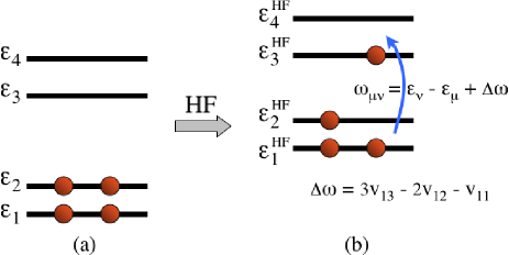
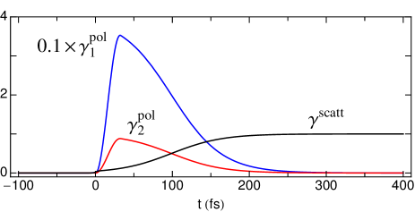
Figure 2: Upper panel: (a) non–interacting energy levels $\epsilon_{1}=0$, $\epsilon_{2}=0.1$, $\epsilon_{3}=1.0$, $\epsilon_{4}=1.3$ and (b) HF energy levels $\epsilon_{\mu}^{\rm HF}=\epsilon_{\mu}+\sum_{\alpha}f^{\rm eq}_{\alpha}(2v_{\mu\alpha}-\delta_{\mu\alpha}v_{\mu\mu})$ with $v_{\mu\mu}=0.4$, $v_{12}=v_{23}=0.2$ and otherwise $v_{\mu\nu}=0.1$ (we recall that $f^{\rm eq}_{\alpha}=\rho^{\rm eq}_{\alpha\alpha}$). The position of the poles $\omega_{\mu\nu}$ of the equilibrium TD-HF $\chi^{\rm eq}(\omega)$ (solution of Eqs. (49-50) with $K_{c}^{\rm eq}=0$) can be calculated analytically and are also indicated. Lower panel: Plot of the damping functions $\gamma^{\rm scatt}(t)$, $\gamma^{\rm pol}_{1}(t)$ (reduced by a factor of 10) and $\gamma^{\rm pol}_{2}(t)$ used in the numerical simulations. Energies $\epsilon_{\mu},\epsilon^{\rm HF}_{\mu}$ and $v_{\mu\nu}$ are in eV while $\gamma^{\rm scatt}$ and $\gamma^{\rm pol}_{1,2}$ are in meV.

The system has filled valence states and empty conduction states at time $t=0$, hence $\rho^{\rm eq}={\rm diag}\{1,1,0,0\}$. The model parameters as well as the HF equilibrium configuration can be found in Fig. 2. For the dipole matrix we use

$$d=d_{0}\left(\begin{array}[]{cccc}0&0&1&1\\ 0&0&1&1\\ 1&1&0&0\\ 1&1&0&0\end{array}\right).$$ (64)

The damping functions $\gamma^{\rm scatt}$ and the two different $\gamma^{\rm pol}=\gamma^{\rm pol}_{1},\gamma^{\rm pol}_{2}$ that we consider are illustrated in the lower panel of Fig. 2. In particular $\gamma^{\rm pol}$ is responsible for the relaxation toward the quasi–stationary density matrix $\rho^{\rm qs}={\rm diag}\{0.9,0.9,0.1,0.1\}$. For the external fields we study a pump pulse of duration $\Delta_{P}=66$ fs and frequency $\omega_{P}=0.6$ eV, and a probe of duration $\Delta_{p}=20$ fs and frequency $\omega_{p}=0.6$ eV; the amplitudes $E_{0}$, $e_{0}$ and $d_{0}$ are chosen to yield $E_{0}d_{0}=0.1$ eV and $e_{0}d_{0}=0.001$ eV.

We calculate $\rho(t)$ in the presence of both pump and probe as well as the probe–free $\tilde{\rho}$ and then extract the probe–induced dipole moment $\delta d(t)=d_{\mu\nu}(\rho_{\nu\mu}(t)-\tilde{\rho}_{\nu\mu}(t))$. Successively, we obtain the transient spectrum of Eq. (14) by Fourier transforming the function $\delta d(t)\times e^{-t/\tilde{\tau}_{p}}$ with $\tilde{\tau}_{p}=80$ fs the life–time of the probe–induced dipole. In the figures below the exponential damping is always included in the probe–induced dipole. The probe–free $\tilde{\rho}$ is also used in Eq. (45) to calculate the adiabatic NEQ response function and hence the transient spectrum according to Eq. (21). The quality of the adiabatic approximation is assessed in different regimes.

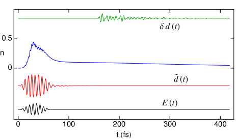
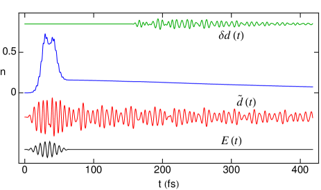
Figure 3: From bottom to top, pump pulse $E(t)$ (black), probe–free dipole $\tilde{d}(t)$ (red), occupation $n_{3}=n_{4}\equiv n$ of valence states (blue) and probe–induced dipole $\delta d(t)$ (green) for the large $\gamma^{\rm pol}_{1}$ (top panel) and small $\gamma^{\rm pol}_{2}$ (bottom panel) damping functions. These results are obtained for a delay $\tau=130$ fs. The quantities $E(t)$, $\tilde{d}(t)$ and $\delta d(t)$ are in arbitrary units.

V.2 Results and discussion

In the upper panel of Fig. 3 we show some relevant quantities obtained from the numerical solution of Eq. (28) with $\gamma^{\rm pol}=\gamma^{\rm pol}_{1}$, namely (from bottom to top) the pump pulse $E(t)$, the probe–free dipole $\tilde{d}(t)$, the time-dependent occupation $n_{3}(t)=n_{4}(t)\equiv n(t)$ of the valence states 3 and 4, and the probe–induced dipole $\delta d(t)$. The behavior of these quantities resemble the behavior in Fig. 1. When the probe arrives ($\tau=130$ fs), the pump-induced polarization is completely dephased ($\tau_{\rm pol}\sim 100$ fs), and the system is slowly moving around the quasi–stationary excited state described by $\rho^{\rm qs}$. In this situation the time-scale over which the one–particle density matrix changes is $T_{P}\sim 1/\gamma^{\rm scatt}\sim 10^{3}$ fs. Since $T_{P}$ is much larger than the life–time $\tau_{p}=\tilde{\tau}_{p}+\Delta_{p}=100$ fs of the dressed probe the adiabatic condition is fulfilled, see Eq. (18).

The transient absorption spectra $\mathfrak{S}^{\tau}(\omega)$ obtained within NEGF according to Eq. (14) and with the NEQ–BSE according to Eq. (21) are displayed in Fig. 4. As expected, the NEQ–BSE approach is very accurate for delays $\tau\lesssim-\tau_{p}$ and $\tau\gtrsim\tau_{\rm pol}$, i.e., when the probe–induced dipole does not overlap the pump-induced polarization. For $\tau\lesssim-\tau_{p}$ the spectrum $\mathfrak{S}^{\tau}(\omega)$ is the equilibrium spectrum with four peaks at energies $\omega_{\mu\nu}=\epsilon_{\nu}-\epsilon_{\mu}+\Delta\omega$ (with $\mu=1,2$, $\nu=3,4$ and $\Delta\omega=3v_{13}-2v_{12}-v_{11}$), thus NEGF and NEQ–BSE obviously agree. For $\tau\gtrsim\tau_{\rm pol}$ the system is in a nonequilibrium state and the condition of adiabaticity matters. The NEQ–BSE well captures the $\tau$-dependent structure of the NEGF spectrum, with the correct bending of the position of the four main absorption peaks towards their equilibrium value for large $\tau$. At first sight, the agreement seems rather good in the overlap region $-\tau_{p}<\tau<\tau_{\rm pol}$ too. However, in this region $\mathfrak{S}^{\tau}(\omega)$ is very small due to the sizable broadening induced by the large $\gamma^{\rm pol}_{1}$, and a more careful comparison between the NEQ–BSE and NEGF spectra reveals some discrepancies (not shown).

A second simulation has been performed using the smaller damping function $\gamma^{\rm pol}=\gamma^{\rm pol}_{2}$. In this case the pump-induced polarization $\tilde{d}(t)$ is long–lived, as it can be seen in the lower panel of Fig. 3. After a time $\tau=130$ fs the time–scale $T_{P}$ over which the one–particle density matrix changes is given by the period of the coherent oscillations of $\tilde{d}(t)$ and it is roughly equal to the inverse gap $1/\omega_{23}\approx 10$ fs. Thus the condition of adiabaticity $T_{P}\gg\tau_{p}$ is not fulfilled and no agreement between NEQ–BSE and NEGF is expected. The transient absorption spectra are displayed in Fig. 5 showing that the two approaches differ whenever the probe experiences a sizable $\tilde{d}(t)$, i.e., for $-\tau_{p}<\tau\lesssim 500$. In this region the NEGF spectrum exhibits alternating fringes characterized by a large oscillation of the spectral weight at fixed $\omega$ as a function of $\tau$. These features origin from the nonadiabatic coherent motion of the electrons between valence and conduction states, and hence they are out of reach of the NEQ–BSE approach. Remarkably, however, the NEQ–BSE captures important spectral features even in this strongly nonadiabatic situation, the most prominent feature being the upward bending of the main peaks around $\tau=0$. When the coherence is destroyed by the dephasing, i.e., for $\tau>500$ fs, the NEQ–BSE and NEGF spectra are found to be in excellent agreement.

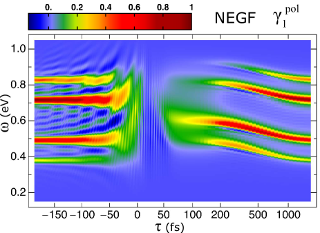
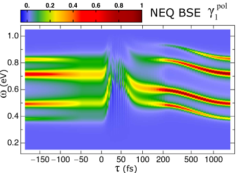
Figure 4: Transient absorption spectrum $\mathfrak{S}^{\tau}(\omega)$ (normalized to its maximum value) obtained within NEGF according to Eq. (14) (upper panel) and with the NEQ–BSE according to Eq. (21) (lower panel) using the damping function $\gamma^{\rm pol}=\gamma^{\rm pol}_{1}$. The peaks of the NEQ–BSE spectrum have been broadened by the inverse life–time $1/\tilde{\tau}_{p}$ of $\delta d(t)$. Notice that the scale of the horizontal axis is linear for $\tau<100$ fs and logarithmic otherwise.

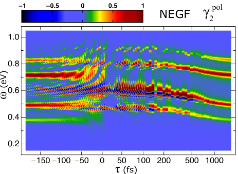
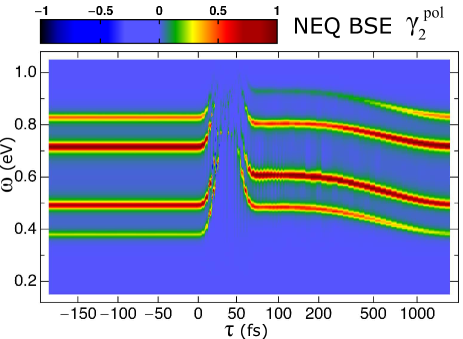
Figure 5: Same as Fig. 4 except that the small damping function $\gamma^{\rm pol}_{2}$ has been used in Eq. (63).

VI Conclusions

We propose a practical method based on MBPT to calculate P&p spectra for delays in the “adiabatic” regime. Starting from the KBE for the Keldysh Green’s function we use the GKBA to obtain an equation of motion for the one–particle density matrix $\rho$ in the presence of both pump and probe fields. Linearization around zero probe yields an equation for the NEQ response function $\chi(t,t^{\prime})$. After the action of the pump we identify a physically relevant regime during which the probe–free density matrix $\tilde{\rho}$ varies on a time-scale much longer than the life–time of the dressed probe. In this regime we make the adiabatic approximation and show that $\chi(t,t^{\prime})$ can be written as a function of the pump-probe delay $\tau$ and of the relative time $(t-t^{\prime})$, i.e., $\chi(t,t^{\prime})\approx\chi^{\tau}(t-t^{\prime})$. This simplification allows us to Fourier transform with respect to the relative time and to derive the main result of this work: a NEQ–BSE that can be implemented in most of the ab–initio  numerical schemes and codes. We further provide a sound physical interpretation of the NEQ response function and showed that it can be related to intrinsic spectral properties of the nonequilibrium system. Well known effects like the renormalization of the band–gap and excitonic binding energies in semiconductors and insulators are naturally explained.

The computational advantage of the NEQ–BSE over NEGF simulations is enormous as only the probe–free one–particle density matrix $\tilde{\rho}$ enters in the solution of the NEQ–BSE. This implies that a single time–propagation is sufficient to obtain the transient spectrum for several delays. In contrast, the NEGF approach requires a time-propagation for every delay (to obtain the one–particle density matrix with pump and probe fields) in addition to the time–propagation to obtain $\tilde{\rho}$. The validity of the NEQ–BSE has been successfully demonstrated in a simple four-level model system and it is currently under investigation in more realistic hamiltonians with encouraging results.

References

- (1) R. Berera, R. van Grondelle and J. T. M. Kennis, Photosynth. Res. 101, 105 (2009).
- (2) G. Sansone, T. Pfeifer, K. Simeonidis and A. I. Kuleff, Chem. Phys. Chem. 13, 661 (2012).
- (3) L. Gallmann, J. Herrmann, R. Locher, M. Sabbar, A. Ludwig, M. Lucchini and U. Keller, Mol. Phys. 111, 2243 (2013).
- (4) A. I. Kuleff and L. S. Cederbaum, J. Phys. B: At. Mol. Opt. Phys. 47, 124002 (2014).
- (5) S. M. Falke, C. A. Rozzi, D. Brida, M. Maiuri, M. Amato, E. Sommer, A. De Sio, A. Rubio, G. Cerullo, E. Molinari and C. Lienau, Science 344, 1001 (2014).
- (6) W. Beenken and V. May, J. Opt. Soc. Am. B 14, 2804 (1997).
- (7) B. Wolfseder, L. Seidner, G. Stock and W. Domcke, Chem. Phys. 217, 275 (1997).
- (8) R. Santra, V. S. Yakovlev, T. Pfeifer and Z. Loh, Phys. Rev. A 83, 033405 (2011).
- (9) A. S. Moskalenko, Y. Pavlyukh and J. Berakdar, Phys. Rev. A 86, 013202 (2012).
- (10) J. C. Baggesen, E. Lindroth and L. B. Madsen, Phys. Rev. A 85, 013415 (2012).
- (11) A. D. Dutoi, K. Gokhberg and L. S. Cederbaum, Phys. Rev. A 88, 013419 (2013).
- (12) E. Perfetto and G. Stefanucci, Phys. Rev. A 91, 033416 (2015).
- (13) Y. Shen, The principles of nonlinear optics (Wiley Series in Pure and Applied Optics, J. Wiley, 1984).
- (14) G. Khitrova, P. R. Berman and M. Sargent III, J. Opt. Soc. Am. B 5, 160 (1988).
- (15) Y. J. Yan and S. Mukamel, Phys. Rev. A 41, 6485 (1990).
- (16) W. T. Pollard and R. A. Mathies, Annu. Rev. Phys. Chem. 43, 497 (1992).
- (17) S. Mukamel, Principles of Nonlinear Optical Spectroscopy (Oxford University Press, Oxford, 1995).
- (18) Y. J. Yan, W. Zhang and J. Che, J. Che. Phys. 106, 2212 (1997).
- (19) G. Strinati, Rivista del Nuovo Cimento 11, 1 (1988).
- (20) G. Stefanucci and R. van Leeuwen, Nonequilibrium Many-Body Theory of Quantum Systems: A Modern Introduction (Cambridge University Press, Cambridge, 2013).
- (21) G. Strinati, H. J. Mattausch and W. Hanke, Phys. Rev. B 25, 2867 (1982).
- (22) G. Onida, L. Reining, and A. Rubio, Rev. Mod. Phys. 74, 601 (2002).
- (23) S. Albrecht, L. Reining, R. Del Sole, G. Onida, Phys. Rev. Lett. 80, 4510 (1998).
- (24) L. X. Benedict, E. L. Shirley, R. B. Bohn, Phys. Rev. Lett. 80, 4514 (1998).
- (25) M. Rohlfing, S. G. Louie, Phys. Rev. Lett. 81, 2312 (1998)
- (26) G. Pal, Y. Pavlyukh, W. Hübner, and H.C. Schneider, Eur. Phys. J. B 79, 327 (2011).
- (27) M. Petersilka, U. J. Gossmann and E. K. U. Gross, Phys. Rev. Lett. 76, 1212 (1996).
- (28) M. E. Casida, in Recent Advances in Density Functional Methods, Part I, edited by D.P. Chong (Singapore, World Scientific, 1995), p. 155.
- (29) E. Runge and E. K. U. Gross, Phys. Rev. Lett. 52, 997 (1984).
- (30) C. A. Ullrich, Time-Dependent Density-Functional Theory: Concepts and Applications (Oxford University Press, 2011).
- (31) C. A. Rozzi, S. M. Falke, N. Spallanzani, A. Rubio, E. Molinari, D. Brida, M. Maiuri, G. Cerullo, H. Schramm, J. Christoffers and C. Lienau, Nat. Comm. 4, 1602 (2013).
- (32) Ch. Neidel, J. Klei, C.-H. Yang, A. Rouzée, M. J. J. Vrakking, K. Klünder, M. Miranda, C. L. Arnold, T. Fordell, A. L’Huillier, M. Gisselbrecht, P. Johnsson, M. P. Dinh, E. Suraud, P.-G. Reinhard, V. Despré, M. A. L. Marques, and F. Lépine, Phys. Rev. Lett. 111, 033001 (2013).
- (33) U. De Giovannini, G. Brunetto, A. Castro, J. Walkenhorst and A. Rubio, ChemPhysChem 14, 1363 (2013).
- (34) N. T. Maitra, F. Zhang, R. J. Cave and K. Burke, J. Chem. Phys. 120, 5932 (2004).
- (35) S. Kümmel and L. Kronik, Rev. Mod. Phys. 80, 3 (2008).
- (36) O. Gritsenko and E. J. Baerends, J. Chem. Phys. 121, 655 (2004).
- (37) N. T. Maitra, J. Chem. Phys. 122, 234104 (2005).
- (38) N. T. Maitra and D. G. Tempel, J. Chem. Phys. 125, 184111 (2006).
- (39) G. Stefanucci and S. Kurth, Phys. Rev. Lett. 107, 216401 (2011).
- (40) S. Kurth and G. Stefanucci, Phys. Rev. Lett. 111, 030601 (2013).
- (41) L. Reining, V. Olevano, A. Rubio and G. Onida, Phys. Rev. Lett. 88, 066404 (2002).
- (42) E. Goulielmakis, Z. Loh, A. Wirth, R. Santra, N. Rohringer, V. S. Yakovlev, S. Zherebtsov, T. Pfeifer, A. M. Azzeer, M. F. Kling, S. R. Leone and F. Krausz, Nature 466, 739 (2010).
- (43) N. Rohringer and R. Santra, Phys. Rev. A 79, 053402 (2009).
- (44) H. Haug and A.-P. Jauho, Quantum Kinetics in Transport and Optics of Semiconductor (Springer-Verlag, Berlin, 1998).
- (45) Here for optically thin we mean that the sample is microscopic along the propagation direction of the light-pulse.
- (46) R. van Leeuwen, N. E. Dahlen, G. Stefanucci, C.-O. Almbladh and U. von Barth, Lect. Notes Phys. 706, 33 (2006).
- (47) P. Danielewicz, Ann. Phys. 152, 239 (1984).
- (48) K. Balzer and M. Bonitz, Nonequilibrium Green’s Functions Approach to Inhomogeneous Systems, Lecture Notes in Physics (Springer-Verlag, Berlin Heidelberg, 2013), Vol. 867.
- (49) L. P. Kadanoff and G. Baym, Quantum Statistical Mechanics (Westview Press, Boulder, CO, 1994).
- (50) P. Lipavský, V. pika and B. Velický, Phys. Rev. B 34, 6933 (1986).
- (51) J. I. Fuks, K. Luo, E. D. Sandoval, and N. T. Maitra, Phys. Rev. Lett. 114, 183002 (2015).
- (52) N. E. Dahlen and R. van Leeuwen, Phys. Rev. Lett. 98, 153004 (2007).
- (53) P. Myöhänen, A. Stan, G. Stefanucci and R. van Leeuwen, Phys. Rev. B 80, 115107 (2009).
- (54) A. Marini, Phys. Rev. Lett. 101, 106405 (2008).
- (55) A. Marini and R. Del Sole, Phys. Rev. Lett. 91, 176402 (2003).
- (56) H. Haug, Phys. Status Solidi B 173, 139 (1992).
- (57) M. Bonitz, D. Semkat, and H. Haug, Eur. Phys. J. B 9, 309 (1999).
- (58) A. Marini, J. Phys. Conf. Ser. 427, 012003 (2013).
- (59) S. Latini, E. Perfetto, A.-M. Uimonen, R. van Leeuwen and G. Stefanucci, Phys. Rev. B 89, 075306 (2014).
- (60) C. Attaccalite, M. Grüning, A. Marini, Phys. Rev. B 84, 245110 (2011).