Spatio-temporal Patterns in Inclined Layer Convection

Abstract

This paper reports on a theoretical analysis of the rich variety of spatio-temporal patterns observed recently in inclined layer convection at medium Prandtl number when varying the inclination angle $\gamma$ and the Rayleigh number $R$. The present numerical investigation of the inclined layer convection system is based on the standard Oberbeck-Boussinesq equations. The patterns are shown to originate from a complicated competition of buoyancy-driven and shear-flow driven pattern forming mechanisms. The former are expressed as longitudinal convection rolls with their axes oriented parallel to the incline, the latter as perpendicular transverse rolls. Along with conventional methods to study roll patterns and their stability, we employ direct numerical simulations in large spatial domains, comparable with the experimental ones. As a result, we determine the phase diagram of the characteristic complex 3D convection patterns above onset of convection in the $\gamma-R$ plane, and find that it compares very well with the experiments. In particular we demonstrate that interactions of specific Fourier modes, characterized by a resonant interaction of their wavevectors in the layer plane, are key to understanding the pattern morphologies.

1 Introduction

Pattern forming instabilities in macroscopic dissipative systems, driven out of equilibrium by external stresses, are common in nature and have been studied intensely over the last decades (see e.g. Cross & Hohenberg (1993)). Prominent examples are found in fluid systems (see e.g. Chandrasekhar (1961), Swinney & Gollub (1985)) where the pattern formation is driven either thermally or by shear stresses. The general understanding of pattern forming systems has benefited from numerous experimental and theoretical investigations of the classical, thermally driven Rayleigh-Bénard convection (RBC) in a layer of a simple fluid heated from below (Busse, 1989; Bodenschatz, Pesch & Ahlers, 2000; Lappa, 2009). In the RBC system, the main control parameter is the Rayleigh number, $R$, a dimensionless measure of the applied temperature gradient. At a critical Rayleigh number, $R_{c}$, the quiescent heat-conducting basic state develops into the well-known periodic arrays of convection rolls characterized by a critical wavevector $\bm{q}_{c}$. The stability of the rolls and their evolution towards characteristic 3D patterns via sequences of bifurcations with increasing $R$ has been investigated by Busse and coworkers (see e.g. Cross & Hohenberg (1993); Busse & Clever (1996) and references therein). The present paper analyzes a variant of RBC, the inclined layer convection (ILC) system, where the fluid layer is inclined at an angle $\gamma$ to the horizontal. Investigations of this system also have a long tradition (see e.g. Vest & Arpaci (1969); Gershuni & Zhukhovitzkii (1969); Hart (1971); Bergholz (1977); Ruth et al. (1980); Fujimura & Kelly (1992); Daniels et al. (2000)).

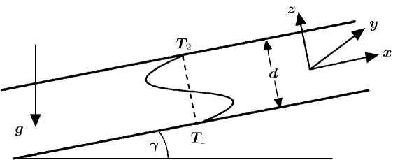
Figure 1: Inclined convection cell of thickness $d$ which is heated from below and cooled from above with temperature difference $\Delta T\equiv T_{1}-T_{2}>0$ for the inclination angle $0^{\circ}\leq\gamma\leq 90^{\circ}$. Driven by gravity $\bm{g}$ the cold fluid flows downwards near the top plate and the hot fluid flows upwards near the bottom plate in the form of a cubic velocity profile (2). For the range $90^{\circ}<\gamma<180^{\circ}$, the fluid layer is inverted and is heated from above.

In the ILC system, for $\gamma\neq 0^{\circ}$ gravity $\bm{g}$ has components both perpendicular and parallel to the fluid layer, which leads to an important modification of the basic state compared to RBC. The applied temperature gradient first produces stratified fluid layers with continuously varying temperatures and densities. In addition, the basic state already contains a flow field driven by the in-plane component of $\bm{g}$: the heavier (colder) fluid will flow down the incline and the lighter (warmer) fluid will flow upwards. Since the resulting flow field creates a velocity gradient perpendicular to the fluid layer, both buoyancy and shear stress driven instabilities of the basic state compete. Their relative importance is governed by the Prandtl number Pr, the ratio of the thermal diffusivity, $\kappa$, to the kinematic viscosity, $\nu$, of the fluid. Furthermore, the strength of the shear stress can be continuously increased by increasing $\gamma$. The orientation of the roll axes at onset of convection allows for directly discriminating between buoyancy and shear driving. The buoyancy driven rolls are aligned parallel to the incline (longitudinal rolls) while the shear driven rolls are aligned perpendicular to the incline (transverse rolls). It should be noted that the latter also bifurcate, when the fluid layer is heated from above and the thermal stress is therefore stabilizing.

Our goal is not a representative parameter study of ILC with respect to $R,\gamma,\mbox{{Pr}}$, which would go beyond the scope of a single paper. Our theoretical investigations have instead been motivated by recent ILC experiments in pressurized $\mathrm{CO_{2}}$ (Daniels et al., 2000; Bodenschatz et al., 2000) with a fixed value $\mbox{{Pr}}=1.07$ of the Prandtl number. In this work the $R-\gamma$ parameter space has been systematically explored and a variety of fascinating patterns have been described. As in all ILC studies mentioned above, our theoretical analysis is based on the Oberbeck-Boussinesq equations (OBE). In contrast to the extensively studied RBC, earlier results in the literature for the ILC system are mostly limited to the linear regime and characterize the primary bifurcation of the convection rolls from the basic state at $R=R_{c}$ (see e.g. Vest & Arpaci (1969); Gershuni & Zhukhovitzkii (1969); Hart (1971); Ruth et al. (1980); Fujimura & Kelly (1992)). In the nonlinear regime ($R>R_{c}$) Busse and Clever (Clever & Busse, 1977; Busse & Clever, 1992) investigated secondary and tertiary instabilities of the convection rolls for some special cases. In contrast, the present work is devoted to a comprehensive theoretical analysis of the patterns in Daniels et al. (2000) at $\mbox{{Pr}}=1.07$.

In the present work we make use of the well-known arsenal of concepts to analyse pattern forming instabilities in fluid systems (see e.g. Cross & Hohenberg (1993)). This approach deploys its full power in large aspect ratio systems (lateral extension, $L$, of the fluid layer much larger than its thickness, $d$) which were first realized experimentally in Daniels et al. (2000). From a linear instability analysis of the basic state we determine the critical values $R_{c},\bm{q}_{c}$ at the onset of convection. The properties of the rolls in the weakly nonlinear regime, $R\gtrsim R_{c}$, are then analyzed in the framework of amplitude equations, which yield approximate roll solutions. Using these as starting solutions allows for the iterative determination of the roll solutions in the nonlinear regime, where $R>R_{c}$. In a further step, their stability is again tested to identify the secondary instabilities of the roll pattern.

We will demonstrate the agreement between experiments and theory with respect to the onset of convection in the $\gamma$-$R$-plane. For inclination angles $\gamma$ below a codimension $2$ angle $\gamma_{c2}\approx 78^{\circ}$ for $\mbox{{Pr}}=1.07$ the destabilisation of the basic state is driven by longitudinal rolls, while transverse rolls bifurcate for $\gamma>\gamma_{c2}$. Both bifurcations are always stationary and continuous (supercritical). The subsequent secondary destabilisation of the 2D rolls for $\gamma\neq 0^{\circ}$ at increasing $R$ is driven by oblique roll solutions, whose axes are not along the longitudinal or transverse roll directions. As a result, spatially periodic 3D patterns are often observed. These are characterized by the nonlinear interaction of three roll modes with wave vectors ($\bm{q}_{1},\bm{q}_{2}\textrm{~{}and~{}}\bm{q}_{3}$), that fulfil a wavevector resonance condition $\bm{q}_{1}+\bm{q}_{2}+\bm{q}_{3}=0$.

As common in other large aspect ratio convection experiments, one also finds imperfectly periodic, weakly turbulent patterns. For instance, the 3D motifs mentioned above appear locally superimposed on the original the 2D roll pattern, where they burst and vanish repeatedly in time (Daniels et al., 2000; Daniels & Bodenschatz, 2002; Daniels et al., 2003). To test whether such dynamic states are caused by experimental imperfections (e.g. lateral boundaries, spatial variations of the cell thickness, inclination of the cell in two directions), we have performed the first comprehensive numerical simulations of the OBE in ILC for large aspect ratio convection cells. While a conclusive assessment of the underlying mechanism producing bursts remains elusive, the weakly turbulent dynamics of the pattern have been well reproduced in our simulations. Since the shear stresses play an important role in our system, there might be an analogy to the instabilities of the laminar state in purely shear driven fluid systems like Couette or Poisseuille flow, which also often appear in the form of localized events (for recent examples see e.g. (Lemoult et al., 2014; Tuckerman et al., 2014)). We hope that investigations such as this one will reveal deeper commonalities between ILC and such shear driven patterns in the future.

The paper is structured as follows: a brief summary of the governing OBE for the ILC system is given in §2. We then discuss the onset of convection in terms of $\bm{q}_{c},R_{c}$ for $\mbox{{Pr}}=1.07$ and the resulting periodic roll pattern in §3. The results of the stability analysis of the rolls the nonlinear regime and the resulting phase diagram are presented in §4. In §5 we show direct simulations of the OBE for different $R$ and $\gamma$, which compare well with the experiments. A short summary of this work together with perspectives for future work can be found in §6. In three detailed appendices we present first the detailed OBE equations for the ILC system and discuss the numerical method to characterize the roll solutions above onset together with their secondary instabilities (Appendix A). Then we address briefly our approach to solve the OBE in general using direct numerical simulations (Appendix B). Finally we return to the linear stability analysis of the basic state to give additional informations regarding the properties of $\bm{q}_{c},R_{c}$ (Appendix C).

2 Oberbeck-Boussines equations for ILC

As shown in figure 1, we consider convection in a fluid layer of thickness $d$, which is inclined at an angle $\gamma$ ($0^{\circ}<\gamma<180^{\circ}$) with respect to the horizontal. Constant temperatures $T_{2}$ ($T_{1}$) with difference $\Delta T=T_{1}-T_{2}>0$ are prescribed at the boundaries ($z=\pm d/2)$ of the layer. Both cases, heating from below ($0^{\circ}<\gamma\leq 90^{\circ}$) and heating from above ($90^{\circ}<\gamma<180^{\circ}$), will be considered in this paper.

The resulting ILC system is described by the standard Oberbeck-Boussinesq equations (OBE) for incompressible fluids. As usual, the OBE are non-dimensionalized using $d$ as the length scale and the vertical diffusion time $t_{v}={d^{2}}/{\kappa}$ as the time scale. The velocity $\bm{u}$ is measured in units of $d/t_{v}$ and the temperature $T$ in units of $T_{s}={\nu\kappa}/{\alpha gd^{3}}$ with $\alpha$ the thermal expansion coefficient. Using a Cartesian coordinate system aligned with the layer (see figure 1), the OBE read as follows:

$$\left[{\partial}/{\partial t}+(\bm{u}\cdot\bm{\nabla})\right]T =\nabla^{2}T+R\hat{\bm{z}}\cdot\bm{u},$$ (1a)

$$\mbox{{Pr}}^{-1}\left[{\partial}/{\partial t}+(\bm{u}\cdot\bm{\nabla})\right]\bm{u} =\nabla^{2}\bm{u}-\frac{\bm{g}}{g}T-\bm{\nabla}p\,,$$ (1b)

where $\bm{\nabla}\cdot\bm{u}=0$ due to incompressibility and $\bm{g}=-g\left(\cos\gamma\hat{\bm{z}}+\sin\gamma\hat{\bm{x}}\right)$ describes the effect of gravity with the gravitational constant $g$. All terms which can be expressed as gradients are included in the pressure term $\bm{\nabla}p$. Equations (1) are characterized by the angle of inclination $\gamma$ along with two nondimensional parameters, the Prandtl number $\mbox{{Pr}}=\nu/\kappa$ and the Rayleigh number $R=\Delta T/T_{s}$.

In line with previous theoretical investigations of ILC in the literature (see in particular (Clever & Busse, 1977; Busse & Clever, 1992)), we idealize the system to be quasi-infinite in the $x-y$ plane. This is considered to be the appropriate description for large aspect-ratio systems. Equations (1) then admit primary (basic) solutions (denoted with subscript $0$) of a linear temperature profile $T_{0}(z)$ and cubic shear velocity profile $\bm{U}_{0}(z)$:

$$T_{0}(z)=R\left[\frac{T_{1}+T_{2}}{2\Delta T}-z\right],\,\,\bm{U}_{0}(z)=\hat{\bm{x}}\sin\gamma R\frac{z}{6}\left[z^{2}-\frac{1}{4}\right]\equiv\hat{\bm{x}}\sin\gamma RU^{x}_{0}(z).$$ (2)

It is convenient to introduce modifications $\theta$ and $\bm{v}$ of the basic state and describe the secondary convective state as:

$$T(\bm{x},z,t)=T_{0}(z)+\theta(\bm{x},z,t)\textrm{,}\quad\bm{u}(\bm{x},z,t)=\bm{U}_{0}+\bm{v}(\bm{x},z),\,\,\bm{x}=(x,y),$$ (3)

which fulfill the boundary conditions $\theta(z=\pm 1/2)=\bm{v}(z=\pm 1/2)=0$. Furthermore, the solenoidal velocity field $\bm{v}$ is mapped by the well-known poloidal-toroidal decomposition to two scalar velocity functions $f,\Phi(\bm{x},z,t)$ and a correction $\bm{U}(z,t)$ of $\bm{U}_{0}(z)$; for details, see Appendix A. The resulting coupled set of equations for $\theta,f,\Phi,\bm{U}$ are analyzed in the following sections using standard Galerkin methods and direct numerical simulations (DNS).

3 Finite-amplitude roll solutions

Spatially periodic convection roll solutions of the OBE (1) with wavevector $\bm{q}$ exist for Rayleigh numbers $R>R_{c}$, where the homogeneous basic state (2) is unstable against infinitesimal perturbations which depend on $x,y$. The onset of convection in ILC system at the critical Rayleigh number $R_{c}$, associated with the critical wavevector $\bm{q}_{c}$, has been discussed in Gershuni & Zhukhovitzkii (1969); Birikh et al. (1972); Hart (1971). A very useful overview can be found in Chen & Pearlstein (1989) and references therein. Some additional general information is given in Appendix C.

Since the ILC system is anisotropic, we have to consider the linear stability of the basic state against arbitrarily-oriented convection rolls with wavenumbers $\bm{q}=q(\cos\psi,\sin\psi)$. For that purpose, we have to analyse (1) linearized about the basic state (2). For details of the standard numerical method, see Appendix A.1. For $\gamma=0$ (horizontal layer with $\bm{U}_{0}\equiv 0$) the system is isotropic and we have the standard Rayleigh-Bénard convection (RBC) where $|\bm{q}_{c}|=q_{c0}=3.1163$ and $R_{c}=R_{c0}=1707.762$ (see e.g. Dominguez-Lerma et al. (1984)) which depend on neither $\psi$ nor Pr. This is distinct from finite $\gamma$, since $\bm{U}_{0}(z)$ defined in (2) yields a contribution proportional to $\cos\psi\sin\gamma/\mbox{{Pr}}$ in the linear equations (see 12b).

In the following, we concentrate on the special case $\mbox{{Pr}}=1.07$, where the bifurcation of the basic state is always stationary; other Pr are briefly discussed In Appendix C.2. Figure 2 displays the rescaled critical Rayleigh number $R_{c}/R_{c0}$ and the critical wavenumber $q_{c}$ as function of the inclination angle $\gamma$ and different $\psi$. In general, only two particular $\bm{q}-$orientations turn out to be relevant (see e.g. Appendix C.2). The convection solutions at onset are either buoyancy driven longitudinal rolls with their axes along the incline, i.e. $\bm{q}_{c}=q_{c}\hat{\bm{y}},~{}\psi=90^{\circ}$ or shear driven transverse rolls with their axis perpendicular to the incline where $\bm{q}_{c}=q_{c}\hat{\bm{x}},~{}\psi=0^{\circ}$.

Longitudinal rolls ($\psi=90^{\circ}$) exist only in the range $0<\gamma<90^{\circ}$ (heating from below, see figure 1). Their critical wavenumber is given by $q^{l}_{c}=q_{c0}$ for all $\gamma$ and the critical Rayleigh number $R_{c}^{l}(\gamma)$ fulfils the relation $R^{l}_{c}(\gamma)\cos\gamma=R_{c0}$ (see Appendix C.2), implying that $R^{l}_{c}$ diverges in the limit $\gamma\rightarrow 90^{\circ}$. In contrast, a bifurcation to transverse rolls exists in the whole interval $0<\gamma<180^{\circ}$. The critical Rayleigh number $R^{t}_{c}(\gamma)$ rises continuously as function of $\gamma$ and diverges at $\gamma=180^{\circ}$ (stable horizontal fluid layer, heated from above). In figure 2 the critical data have been shown only for $\gamma$ up to $120^{\circ}$, where $R^{t}_{c}\sim 10^{5}$ involves large thermal gradients. Thus, the use of the OBE becomes questionable for $\gamma>120^{\circ}$, since non-Boussinesq effects due to temperature variation of the various material parameters should be taken into account.

Inspection of figure 2 reveals the existence of a codimension-2 bifurcation point $\gamma_{c2}=77.746^{\circ}$ where $R_{c}^{l}=R^{t}_{c}=8046.420$, such that for $\gamma<\gamma_{c2}$ longitudinal rolls bifurcate at onset ( $R_{c}^{l}<R^{t}_{c}$) while for $\gamma>\gamma_{c2}$ the transverse ones prevail. As first demonstrated in Gershuni & Zhukhovitzkii (1969) and detailed in Appendix C.2, the threshold curves $R^{ob}_{c}(\gamma,\psi)$ for general oblique rolls ($\psi\neq 90$) can be constructed by suitable transformations of the critical values $R^{t}_{c}(\gamma)$ and $q^{t}_{c}(\gamma)$ of the transverse rolls. In this paper, we will often use the reduced main control parameter $\epsilon$ defined as:

$$\epsilon=(R-R_{c}(\gamma,\mbox{{Pr}}))/R_{c}(\gamma,\mbox{{Pr}})$$ (4)

as a measure for the relative distance from threshold $R_{c}(\gamma)$ at $\epsilon=0$, instead of $R$.

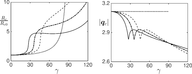
Figure 2: Normalized critical Rayleigh number $R_{c}/R_{c0}$ (left panel) and critical wave number $|\bm{q}_{c}|$ (right panel) as function of the inclination angle $\gamma$ for $\mbox{{Pr}}=1.07$ for different roll orientations $\psi$. Dotted line is for $\psi=90^{\circ}$ (longitudinal rolls), dashed line for $\psi=60^{\circ}$, dashed-dotted line for $\psi=45^{\circ}$ and solid line for $\psi=0^{\circ}$ (transverse rolls).

The standard computational methods to construct finite-amplitude roll solutions with wavevector $\bm{q}_{c}$ for $R>R_{c}$, where exponential growth of the linear modes is balanced by the nonlinear terms in the OBE, are sketched in Appendix A.2. The amplitudes of the roll solutions grow continuously like $\sqrt{\epsilon}$ (see the discussion after (16)). Thus, the primary bifurcation to rolls is continuous (forward).

4 Secondary instabilities of roll solutions for Pr= 1.07

In this section, we discuss the secondary destabilisation mechanism of rolls with wavevector $\bm{q}_{c}$, in a ILC system with $\mbox{{Pr}}=1.07$ and inclination angle $\gamma$, that become unstable when $\epsilon=\epsilon_{inst}(\gamma)$. Based on the methods described in Appendix A.2, the stability diagram presented in figure 3 has been determined in the $\gamma-\epsilon$ plane.The solid lines mark the locations of the various secondary instabilities of the finite amplitude roll solutions with $\bm{q}=\bm{q}_{c}(\gamma)$ at $\epsilon=\epsilon_{inst}(\gamma)$. Thus to the left of this line for $\gamma\approx 15^{\circ}$ and below this line for larger $\gamma$ stable roll solutions exist. For details of the dependence of these secondary stability lines upon cut-off parameters in the Fourier-Galerkin expansions see Appendix A.3.

According to figure 3, the type of secondary roll instabilities depends strongly on the inclination angle $\gamma$. Our main interest in this paper are the various $3D$ patterns which develop for $\epsilon>\epsilon_{inst}$. As a first impression, we include in figure 3 excerpts of patterns observed in experiments (Daniels et al., 2000). Here, we aim to reproduce and interpret such $3D$ patterns based on direct numerical simulations (DNS) of the OBE. For details of time stepping scheme we refer to the algorithm presented in Appendix B.

We first consider small $\epsilon<\epsilon_{inst}(\gamma)$. Starting from random initial conditions, modes with wave vector $\bm{q}_{c}(\gamma)$ prevail leading to perfect roll patterns, as shown in figure 4. The DNS are performed on a square with side lengths $L_{x}=L_{y}=12\lambda_{c}$ with $\lambda_{c}=2\pi/qc(\gamma)$ where we obtain, longitudinal rolls at $\gamma=10^{\circ}$ and transverse rolls at $\gamma=85^{\circ}$. Here, and in the rest of this paper, we show snapshots of the vertical ($z$) average $\langle\theta(\bm{x},t)\rangle$ of the temperature field $\theta(\bm{x},z,t)$ (see (13)). Throughout this paper the height of the convection cell increases from left to right, i.e. with increasing $x$ with respect to the coordinate system attached to the cell (see figure 1). Such pictures, which we refer to as the temperature plots, are typically used in the literature to compare with experimental convection patterns, which are visualized via shadowgraphy (for examples, see Bodenschatz et al. (2000)). In gas convection experiments of the type considered in this paper, dark and bright regions in figure 4 indicate positive (hot) and negative (cold) variations in the temperature field around the basic linear temperature profile (de Bruyn et al., 1996). We use a 8-bit grayscale to visualize $\langle\theta(\bm{x})\rangle$; whose range increases monotonically as a function of $\epsilon$.

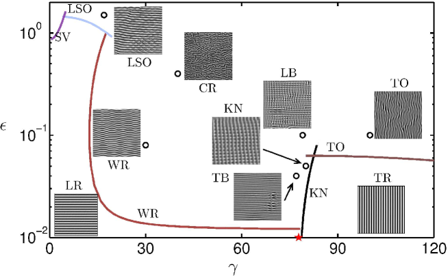
Figure 3: Phase diagram of the convective roll patterns in the $\gamma,\epsilon$ plane for $\mbox{{Pr}}=1.07$. Solid lines (coloured online) indicate the secondary instabilities of the primary roll patterns at $\epsilon=\epsilon_{inst}$, i.e. at $R=(1+\epsilon_{inst})R_{c}(\gamma)$. The codimension 2 point with $\gamma_{c2}=77.746^{\circ}$ is marked by a star. For $\gamma<\gamma_{c2}$, we obtain longitudinal rolls (LR), and for $\gamma>\gamma_{c2}$, transverse rolls (TR). Increasing $\gamma$ in the interval $0\leq\gamma<\gamma_{c2}$, we obtain the thresholds for skewed varicose instability (SV) shown in purple, longitudinal subharmonic oscillations (LSO) shown in light blue and wavy rolls (WR) shown in dark red as instabilities of the LR. In the range $\gamma>\gamma_{c2}$ the thresholds for instability of the transverse rolls through the knot instability (KN) is shown in black and for the transverse oscillations (TO) in brown. The graph is decorated with excerpts from corresponding experimental pictures (Daniels et al., 2000). In addition crawling rolls (CR), transverse (TB) and the longitudinal bursts (LB) are shown, which cannot be directly associated to the secondary instabilities. Black open circles indicate locations in the $\gamma-\epsilon$ plane, where experiments and numerical simulations are compared in section §5.

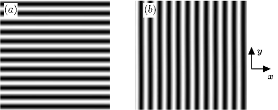
Figure 4: Temperature plots $\langle\theta(\bm{x})\rangle$, for $\mbox{{Pr}}=1.07$ from direct numerical simulations of the OBE (1): ($a$) buoyancy dominated longitudinal rolls oriented along the incline from right to left at $\mbox{{Pr}}=1.07$, $\epsilon=0.01$, $\gamma=10^{\circ}$ with $\bm{q_{c}}=(0,3.1163)$ (left panel); ($b$) shear dominated transverse rolls oriented perpendicular to the incline at $\epsilon=0.02$, $\gamma=85^{\circ}$ with $\bm{q_{c}}=(2.82,0)$ (right panel). In the plane the figures are oriented along the x-axis of local coordinate system in figure 1 (reproduced at the right). All temperature plots in the rest of the paper are shown using the same convention.

In the following, we discuss the secondary instabilities of the primary convection rolls in detail. We start with inclination angles $\gamma$ below $\gamma_{c2}$ in §4.1, before we concentrate on the vicinity of $\gamma_{c2}$ and finally on larger $\gamma$.

The various secondary instabilities are visualized by direct simulations of the underlying OBE (see Appendix B.1). In general we use a minimal rectangular integration domain in the $x-y$ plane which is consistent with $\bm{q}_{c}$ and the wavevectors of the dominant destabilizing modes. For visualisation, the domain is periodically extended to a larger domain with $Lx=12\lambda_{c}=L_{y}$.

4.1 Secondary roll instabilities below $\gamma_{c2}$

In this section, we will characterize in detail the secondary instabilities of longitudinal rolls in figure 3.

4.1.1 Skewed varicose instability (SV)

For small inclinations ($\gamma\lesssim 5^{\circ}$), we recover the well known skewed varicose (SV) instability for planar RBC with $\gamma=0$ (Busse & Clever, 1979). This is a stationary long-wavelength instability where the original longitudinal rolls are slowly modulated along their axes but also with respect to their distance. The SV instability will not be further discussed in this paper.

4.1.2 Logitudinal subharmonic oscillations (LSO)

Figure 5: Subharmonic oscillatory instability of longitudinal rolls (LSO) for $Pr=1.07$, $\gamma=17^{\circ}$ and $\epsilon=1.3$: temperature plot (left panel) together with the wavevectors $\bm{q}_{1}=\bm{q}_{c},\bm{q}_{2},\bm{q}_{3}$ (wavevector resonance $\bm{q}_{1}=\bm{q}_{2}+\bm{q}_{3}$) of the leading Fourier modes (right panel).

.

In the range $5^{\circ}<\gamma\leq 21^{\circ}$, the longitudinal roll pattern with $\bm{q}=\bm{q}_{c}=(0,3.1163)$ becomes linearly unstable to oscillatory subharmonic perturbations with wavevectors $\bm{q}_{2,3}=(\pm q_{x},q_{c}/2)$ and a finite circular frequency $\omega_{inst}$. For the representative case $\gamma=17^{\circ}$, where primary rolls get unstable at $\epsilon_{inst}=1.044$, we have $q_{x}=1.279$ and $\omega_{inst}=10.21$. In figure 5, we show an excerpt from our simulation at $\epsilon=1.3$. performed on the minimal rectangle with sidelengths $L_{x}=2\pi/q_{x}$ and $L_{x}=2\lambda_{c}/q_{c}$ with $\lambda_{c}=2\pi/q_{c}$. The periodically extended picture is six times larger. The pattern is characterized by periodic modulations of the longitudinal rolls, which are in phase on every second roll reflecting the subharmonic nature of the instability. The resulting LSO pattern obeys the wavevector resonance $\bm{q}_{1}-\bm{q}_{2}-\bm{q}_{3}=0$ as seen in the Fourier spectrum.

The time evolution of the pattern in the $x-y$plane is:

$$f(x,y)=A\cos(q_{c}y)+B(t)\cos(q_{x}x+q_{c}y/2)+C(t)\sin(q_{x}x-q_{c}y/2)$$ (5)

The coefficient $A$ is independent of time while $B(t)$ and $C(t)$ are periodic with circular frequency $\omega\approx\omega_{inst}$. The time evolution of these coefficients (given in units of $T_{s}=O(1mK)$ defined in §2) are shown in figure 6.

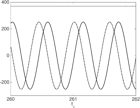
Figure 6: The coefficients $A$ (horizontal upper dotted line), $B(t)$ (dash-dotted) and $C(t)$ (solid line) in (5) as function of time in units of $T_{s}$; $B(t),C(t)$ are multiplied by a factor of four for better visualisation.

The LSO instability has been first described by Busse & Clever (2000) at the lower Prandtl numbers $\mbox{{Pr}}=0.7$, by solving (15) in the minimal integration domain. In addition for certain parameter combinations of $q_{x},q_{y}$ an intermittent appearance of bursts has been described, which we have not reproduced for $\mbox{{Pr}}=1.07$.

4.1.3 Wavy Roll (WR) instabilities

The next instability type, characterized by the appearance of longitudinal rolls undulating like snakes along their axes, has been first described in Clever & Busse (1977) where the notion wavy-instability has been coined. The resulting bifurcation to wavy rolls (WR) is observed in a fairly large $\gamma$-interval between $21^{\circ}<\gamma\leq\gamma_{c2}$, very close to onset of convection ( $\epsilon_{inst}=O(0.01)$). In the framework of the Galerkin stability analysis in Appendix A.2, this instability is characterized by long-wavelength destabilizing modes with wavevectors $\bm{q}_{max}=(\pm q_{x},q_{c})$ with ($|q_{x}|\ll|\bm{q}_{c}|$).

The WR have been discussed in detail in Daniels et al. (2008), to which we refer for details. Here one finds representative experimental and theoretical pictures (see also figure 13 in §5 below) as well as a Galerkin stability analysis of the 3D wavy roll patterns. In fact, for $\epsilon>\epsilon_{inst}$ stable WR with finite $q_{x}$ exist. They are spatially periodic in the plane, characterized by the wavevector resonance $\bm{q}_{2}+\bm{q}_{3}=2\bm{q}_{c}$ with $\bm{q}_{2,3}=(\pm q_{x},q_{c})$. In the $x,y-$plane the temperature pattern is described as

$$f(x,y)=A\cos(q_{c}y)+B\sin(q_{c}y)\sin(q_{x}x).$$ (6)

For $\epsilon=0.1$ and $q_{x}=1.28$, we find for instance $A=48.1$ and $B=12.8$ in units of $T_{s}$.

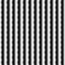
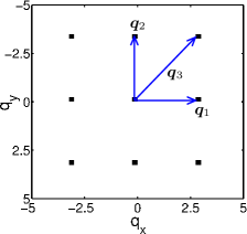
Figure 7: Knot instability of transverse rolls at $Pr=1.07$, $\gamma=81.9^{\circ}$ and $\epsilon=0.055$: temperature plot (left panel); wavevectors of the leading Fourier modes $\bm{q}_{1}=\bm{q}_{c}$, $\bm{q}_{2}=(0,q_{c0})$ and ${\bf{q}}_{3}\,=\,{\bf{q}}_{1}+{\bf{q}}_{2}$ (right panel).

4.2 Secondary roll instabilities above $\gamma_{c2}$

In this section we discuss the secondary instabilities of the transverse rolls bifurcating for inclinations $\gamma>\gamma_{c2}$.

4.2.1 Knot (KN) instability

Just above the codimension 2 point, the shear dominated transverse rolls with $\bm{q_{1}}=(q_{c},0)$ and $q_{c}\simeq 2.82$ (see figure 2) are destabilized by the longitudinal rolls with wavevector $\bm{q}_{2}=(0,q_{y})$ and $q_{y}=q_{c0}=3.1163$. The steeply rising stability line starts at $\gamma=\gamma_{c2}$ at $\epsilon=0$. In view of the logarithmic $\epsilon$-scale, the curve is only shown for $\epsilon>0.01$. In the weakly nonlinear regime, the oblique mode with wave vector $\bm{q}_{3}=(q_{c},q_{y})$ is already important and the wavevector resonance $\bm{q}_{3}\,=\,\bm{q}_{1}+\bm{q}_{2}$ is established. The pattern is well described by:

$$f(x,y)=A\cos(q_{c}x)+B\sin(q_{y}y)+C\sin(q_{c}x)\cos(q_{y}y)$$ (7)

As a function of $\epsilon$, the amplitudes $B,C$ increase continuously above $\epsilon=\epsilon_{inst}$.

In figure 7 we address an representative example for $\gamma=81.9^{\circ}$ with $\epsilon_{inst}=0.053$, where originally $Lx=\lambda_{c}$ and $L_{y}=2\pi/q_{c0}$. At $\epsilon=0.055$, we find $A=17.9,B=1.95,C=2.16$ in (7). The resulting stationary pattern (see figure 7, left panel) has some similarity to the knot patterns described in Busse & Clever (1979) for the isotropic RBC system. However, contrary to the patterns in Busse & Clever (1979), we observe a wavevector resonance triggered by the oblique mode $\bm{q}_{3}$ in the ILC system.

For completeness, it should be mentioned that the knot instability in ILC has been previously investigated in Fujimura & Kelly (1992) for $\gamma\lesssim 90^{\circ}$ in the framework of two coupled amplitude equations restriced to the amplitudes $A,B$ in (7).

4.2.2 Transverse Oscillatory rolls (TO)

For $\gamma>83.2^{\circ}$ the destabilization of the transverse rolls starts to be governed by the transverse oscillatory rolls (TO) along an almost horizontal transition line as function of $\gamma$. Transverse oscillatory rolls (TO) are characterized by destabilizing modes with a Floquet vector $\bm{s}$ of relatively small but finite modulus $|\bm{s}|\sim q_{c}/6$ and by an oscillatory time dependence of period about $3.5t_{v}$. In an analogy to the stationary SV instability of longitudinal rolls (see §4.1.1), the rolls are expected to become slowly modulated along their axis and also with respect to other in-plane direction. Without a definitive resonance condition among the dominant destabilizing modes, we do not expect periodic 3D patterns of the kind discussed in the previous subsections. Thus, we have to solve the OBE on a larger domain in the $x-y$ plane, including modes with wave vectors $|(q_{x},q_{y})|\ll q_{c}$. An excerpt of representative DNS pattern for $\gamma=84.9^{\circ}$ is shown in figure 8 (left panel) at $\epsilon=0.07$. This pattern results from a secondary instability of transverse rolls ($R_{c}=8282.64$ and $q_{c}=2.8023$) at $\epsilon_{inst}=0.063$ with $\omega_{inst}=1.809$. One observes the appearance of localized patches with reduced amplitudes on top of the original slowly modulated transverse rolls. Apparently, the pattern arises through a complex beating phenomena, due to a superposition of oscillating modes with slightly different wave vectors. The most prominent ones ($\bm{q}_{2},\bm{q}_{3}$) together with $\bm{q}_{1}\equiv\bm{q}_{c}$ are shown in figure 8 (right panel).

Figure 9 shows the complicated evolution of the pattern during one cycle ($2\pi/\omega_{inst}$). The localized patches of reduced amplitudes in figure 9(i), evolve into slanted lines of reduces amplitudes in (ii). Further in the cycle, the undulation amplitude of the rolls first increases and decreases then before arriving again at the initial pattern in figure 9(iii-vi).

According to our phase diagram in figure 3, the instability of the transverse rolls towards the TO pattern remains relevant for larger $\gamma$ and also governs the secondary instability in the case of heating from above. A representative example of a time sequence is shown in figure 10 for $\gamma=100^{\circ}$, where the TO instability is characterized by $\epsilon_{inst}=0.06$ and $\omega_{inst}=1.48$. The graph of the most relevant destabilizing modes looks practically identical to the one in figure 8 and is thus not shown. The interaction of the modes leads, however, to a much simpler time evolution, as compared to figure 9 for $\gamma=84.9^{\circ}$. It is possible that in the latter case, the destabilizing modes triggering the knot instability for slightly smaller $\gamma$ in figure 3 come into play as well.

As will be discussed in §5, the regions of suppressed amplitudes become elongated and are no longer periodically arranged in the plane for increasing aspect ratio ($L_{x},L_{y}$). As shown in figure 18 below, they compare well with the corresponding experimental patterns in (Daniels et al., 2000), called switching diamond panes (SDP) there.

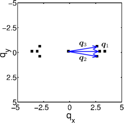
Figure 8: Transverse oscillatory rolls at $Pr=1.07$, $\gamma=84.9^{\circ}$ and $\epsilon=0.07$: temperature plot (left panel); wave vectors of the dominant Fourier modes (right panel). In this case, we use a square grid with $q_{y}=q_{c}=3.117$.

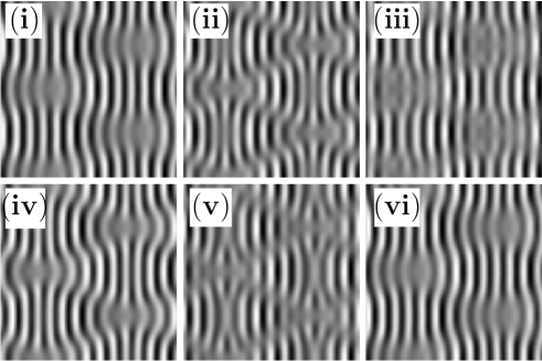
Figure 9: A time sequence of TO patterns shown over one time period for the case of heating from below. Consecutive panels are separated by $0.44t_{\nu}$. System parameters are the same as figure 8 with $Pr=1.07$, $\gamma=84.9^{\circ}$ and $\epsilon=0.07$.

Figure 10: A time sequence of TO patterns shown over one time period for the case of heating from above. Consecutive panels are separated by $0.4t_{\nu}$. System parameters are $Pr=1.07$, $\gamma=100^{\circ}$ and $\epsilon=0.08$.

4.2.3 Vertical convection

The case of a vertical convection cell ($\gamma=90^{\circ}$) is of special interest since the pattern formation is exclusively driven by the shear stress. So this system has motivated many previous investigations, mainly in the linear regime and often with $\mbox{{Pr}}\gtrsim 12.45$ where an oscillatory bifurcation to transverse rolls takes place. For $\mbox{{Pr}}=1.07$, however, we observe stationary transverse rolls at onset, and their stability analysis yields always a secondary bifurcation to the TO pattern for all $\gamma$ near $90^{\circ}$ (see figure 3 and our discussion in the previous subsection).

This result is noteworthy, since in the previous literature (Clever & Busse, 1995) for $\mbox{{Pr}}=0.71$ (air) a stationary secondary instability of the transverse rolls driven by the effective subharmonic roll modes with wavevectors $\bm{q}_{2,3}=(q_{c}/2,\pm p)$ was predicted. This finding has been confirmed by our own calculations. The instability of the transverse rolls with $q_{c}=2.8123,R_{c}=5701.2625$ takes place at $\epsilon_{inst}=0.0599$ with $p=1.5898$. These numbers are consistent with those used for direct simulations of the OBE in Clever & Busse (1995) ($R_{c}=5726.9,q_{c}=2.69,p=1.7$ and $\epsilon\gtrsim 0.11$).

In close analogy to the LSO (§4.1.2), the resonance conditions $\bm{q}_{c}=\bm{q}_{2}+\bm{q}_{3}$ holds. To confirm the results of stability analysis we have performed DNS of the OBE on the smallest periodicity domain in the plane compatible with instability data above, i.e. with $L_{x}=2\lambda_{c},L_{y}=\lambda_{c}(q_{c}/p)$. The resulting stationary temperature plot (periodically extended) for $\epsilon=0.064>\epsilon_{inst}$ is shown in figure 11 for $L_{x}=L_{y}=12\lambda_{c}$. Keeping the dominant Fourier modes, the pattern is represented as:

$$f(x,y)=A\cos(q_{c}x)-B\sin(q_{c}x/2)\cos(py)$$ (8)

with $A=131.23,B=60.76$ in units of $T_{s}$; the subharmonic instability of the transverse rolls is obvious from the argument of sine in the second term.

A closer look at the Pr-dependence of the secondary bifuraction of the transverse rolls in this regime shows that for $\mbox{{Pr}}\gtrsim 0.9$ the secondary SHV bifurcation of the transverse rolls is replaced by the TO bifurcation discussed in §4.2.2. This is consistent with our stability analysis and experimental observations at $\mbox{{Pr}}=1.07$.

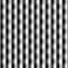
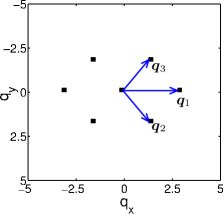
Figure 11: Subharmonic varicose instability of transverse rolls with $\mbox{{Pr}}=0.71$, $\epsilon=0.065$ and $\gamma=90^{\circ}$: temperature plot (left panel); wavevectors of the leading Fourier amplitudes (right panel). Given that $q_{x}=2.8123$ and $q_{y}=1.59$ and choosing the number of rolls $n_{L}=12$, we have $\triangle q_{x}=q_{x}/n_{L}=0.2344$ and $\triangle q_{y}=q_{y}/n_{L}=0.1358$.

5 Comparison with experimental results

In the previous section, we have discussed the various characteristic secondary instabilities of the ILC roll patterns with increasing inclination angle $\gamma$. A number of basic destabilization mechanisms have been identified by considering simulations in small periodicity domains in the plane of linear dimension $L$, where $L=O(2d)$ with $d$ the cell thickness. Our goal in this section is a comparison with the pressurized $\mathrm{CO_{2}}$ experiments (Daniels et al., 2000; Daniels, 2002) at $\mbox{{Pr}}=1.07$. In these experiments a convection cell with very small layer thickness $d=(710\pm 7)\mu$ m could be realized together with quite large lateral dimensions [($42\times 21$)$d^{2}$]. Thus, the dimensions of the convection cell are such that the experiments are expected to be well described in simulations by periodic boundary conditions in the plane. Furthermore, such dimensions give a vertical diffusion time $t_{v}=d^{2}/\kappa=3.0$ s, which sets the time scale, is small enough for typical experiments. In the rest of this section, we will present the generic features of the patterns when all transients have died out. To compare with theory, we have performed numerical simulations of the basic equations (1) on a large horizontal domain with lateral dimension up to $L=20\lambda_{c}=O(40d)$. For the numerical method, see Appendix B.

Excerpts of the experimental shadowgraph pictures to be discussed in this section are already shown in figure 3. We will follow the same sequence of parameter combinations used in the preceding section, where $\gamma$ was systematically increased. As discussed in §4, we show in this section the vertical temperature average $\langle\theta(\bm{x})\rangle$ side by side with the corresponding experiments. A quantitative agreement between theory and experiment is not to be expected, as along with the complicated optics involved in shadowgraphy (Trainoff & Canell, 2002), the experimental pictures are typically digitally remastered to enhance their contrast.

5.1 Convection pattern for $\gamma<\gamma_{c2}$

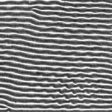
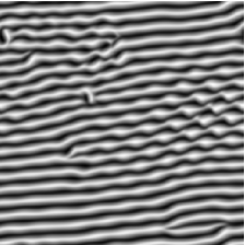
Figure 12: Snapshots of an longitudinal subharmonic oscillations (LSO) for $Pr=1.07$, $\gamma=17^{\circ}$ and $\epsilon=1.5$ from experiments (left panel) and from our numerical simulation (right panel).

We start with the subharmonic oscillatory patterns (LSO), in figure 5 which bifurcate from longitudinal rolls. As shown in figure 12, experiments and theory match very well. We observe patches of subharmonic oscillations, which we have previously discussed in §4.1.2 on the basis of a stability analysis of the longitudinal rolls and numerical simulations in a minimal domain (containing only one roll pair). In large ILC systems, typically such motifs appear only in localized patches that compete with moderately distorted rolls. Such patches expand and shrink in time and their centers move erratically over the plane. The subharmonic oscillations within the localized patches show an internal dynamics with a time scale of 1 to 3 cycles per $t_{v}$ which is of the same order as the period $2\pi/\omega_{inst}$ of the Hopf bifurcation in §4.1.2.

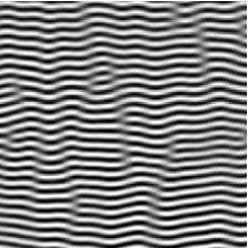
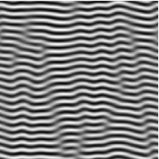
Figure 13: Representative wavy roll patterns (WR) from experiments (left panel) in comparison with simulations (right panel) for $Pr=1.07$, $\gamma=30^{\circ}$ and $\epsilon=0.08$.

With increasing $\gamma$, the longitudinal rolls become unstable against undulations even for very small $\epsilon$; i.e. the instability line in figure 3 bends dramatically down. Typical experimental and theoretical pictures of undulated (wavy) rolls (WR) shown in figure 13 again match very well with each other. However, instead of the stationary undulations as predicted in §4.1.3, the patterns are characterized by patches of uniform undulated rolls, separated by grain boundaries (Daniels et al., 2000; Daniels & Bodenschatz, 2002). In addition, the rolls are scattered with point defects that move at right angles to the rolls. The wavy patterns have been discussed in detail in Daniels et al. (2008), where also a weakly chaotic dynamics of the amplitudes $A,B$ in (6) is analyzed in detail.

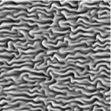
Figure 14: Crawling rolls (CR) from experiments (left panel) and from simulations (right panel) at the same parameters as in figure 13 except at a larger $\epsilon=0.4$.

With increasing $\epsilon$, the undulations become more and more disordered and the rolls get disrupted. A transition is observed to the dynamic state of the so called crawling rolls (CR) Daniels et al. (2000) as shown in figure 14. This state is also obtained in our numerical simulations, which indicates that it is not caused by experimental imperfections.

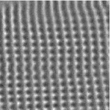
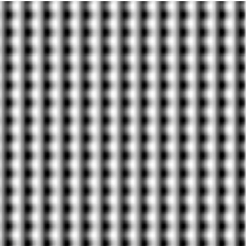
Figure 15: Knot pattern (KN) at $\gamma=80^{\circ}$ and $\epsilon=0.05$ in experiments (left panel) and in simulations (right panel).

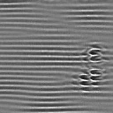
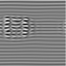
Figure 16: Localized transverse bursts (TB) for the parameters $Pr=1.07$, $\gamma=77^{\circ}$ and $\epsilon=0.04$ in experiments (left panel) and in simulations (right panel).

5.2 Convection close to codimension 2 point

The vicinity of the codimension 2 point $\gamma_{c2}$ is of particular interest. According to figure 3 the wavy roll instability governs the secondary instability of the longitudinal rolls up to $\gamma=\gamma_{c2}$. In contrast, for $\gamma\gtrsim\gamma_{c2}$ the primary transverse rolls are predicted to become unstable against cross rolls leading to the knot patterns (KN). This instability mechanism is confirmed by the pictures shown in figures 15. It is remarkable that the DNS on a large domain in the plane ($L_{x}=L_{y}=20\lambda_{c}$) starting from random initial conditions has led to perfect knot patterns. They are indistinguishable from those shown in figure 7 generated on a small domain with $L_{x},L_{y}\approx\lambda_{c}$. The teeth-like structure on the transverse rolls caused by a resonant interaction of the three roll modes (see figure 7) is born out in the experimental picture. However, the transverse rolls are slightly oblique here and undulated.

We now discuss two types of patterns which do not allow for a direct interpretation by secondary instabilities of the basic rolls. First, we show in figure 16 the transverse bursts (TB) for $\gamma=77^{\circ}\lesssim\gamma_{c2}$ and at $\epsilon=0.04$ slightly above the secondary wavy bifurcation of the longitudinal rolls. Both in experiments and simulations, we observe a background of slightly undulated rolls with some amplitude modulations. Intermittently, localized transverse structures (bursts) appear, which contract, vanish and reappear at other places. The longitudinal bursts in experiments have been analyzed in Daniels et al. (2003), to which we refer for more details.

In contrast, for $\gamma>\gamma_{c2}$ and intermediate $\epsilon$, longitudinal bursts (LB) are observed; representative examples are shown in figure 17. They are characterized by localized loops of longitudinal rolls superimposed on transverse rolls. The experimental picture shows more of the bimodal knot pattern in the background than do the simulations. In the vicinity of $\gamma_{c2}$, we do not expect simulations to reproduce all details of the the experiments at the same parameters, as the system is very sensitive against small changes of $\gamma$ and $\epsilon$. The material parameters in the experiments certainly have some inaccuracies. In addition, non-Boussinesq effects presumably lead to a slow drift of the experimental pattern. Although the two burst phenomena are clearly reflected in our simulations, additional efforts are necessary in the future to understand their underlying mechanism.

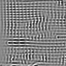
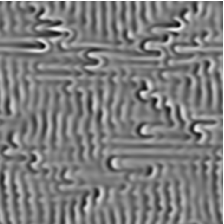
Figure 17: Localized longitudinal bursts (LB) for the parameters $Pr=1.07$, $\gamma=79^{\circ}$ and $\epsilon=0.1$ in experiments (left panel) and in simulations (right panel)

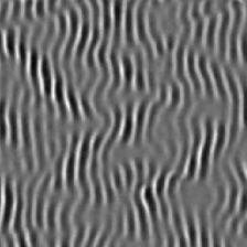
Figure 18: Switching diamond panes (SDP) for the parameters $Pr=1.07$, $\gamma=100^{\circ}$ and $\epsilon=0.1$ in experiments (left panel) and in simulations (right panel).

Figure 19: Patterns formed during a typical evolution of switching oscillatory rolls shown in order, for the case of heating from above as in figure 18. Consecutive panels are separated by $5\,t_{\nu}$. System parameters are $Pr=1.07$, $\gamma=100^{\circ}$ and $\epsilon=0.1$.

5.3 Shear stress dominated instabilities

Finally, we briefly address the heating-from-above case which is described in §3, for which the inclination angle is $\gamma>90^{\circ}$. As discussed before, the destabilization of the basic state is due to the shear stress of the cubic flow profile $\bm{U}_{0}$ (2). In §4.2.2 we have described the destabilisation of the primary transverse rolls to switching diamond pane patterns shown in Daniels & Bodenschatz (2002). According to figure 3, the transition line to the TO is almost horizontal and begins at $\gamma$ slightly above $\gamma_{c2}$. In figure 18, we show a representative example for $\gamma=100^{\circ}$, where experiment and simulations agree very well. The time evolution observed in the corresponding time sequence, presented in figure 19, reflects the frequency $\omega_{inst}=1.48$ given in §4.2.2 and documented in figure 10. Increasing $\epsilon$ further causes the patches with enhanced amplitude to get smaller and to move more erratically as shown in figure 20.

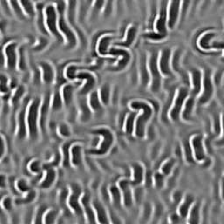
Figure 20: Chaotic switching rolls at $\gamma=100^{\circ},\epsilon=0.19$ [experiments (left panel), simulations (right panel)].

6 Conclusions

The recent experimental study of ILC for $\mbox{{Pr}}=1.07$ by Daniels et al. (2000) has opened a new path to a much better understanding of this dynamically rich system. For a recent overview, see chapter 7 in Lappa (2009). In contrast to previous work, the convection instabilities of the basic state, sketched in figure 1, have been systematically explored as function of the inclination angle $\gamma$ and the Rayleigh number $R$. Furthermore, the resulting patterns are visualized directly and the large variety of new pattern types are shown in the phase diagram in figure 3.

For the theoretical analysis in this paper, the large lateral extent of the convection cell in the experiment has been of particular importance. For large aspect ratio systems the influence of the lateral boundaries of the cell is certainly highly suppressed, making it appropriate to use periodic boundary conditions. A convincing agreement with experiments by Daniels et al. (2000) has been obtained. The analysis of the primary bifurcation of rolls at the onset of convection and their secondary bifurcations have revealed the complicated interaction of buoyancy and shear driven destabilization mechanisms. Of particular importance is the spatially resonant interaction between three roll systems with different orientations in the plane (wavevector resonance, as detailed in §4).

A look at the experimental pictures and the pattern dynamics (see Daniels et al. (2000)) shows that they are not completely described by perfect periodic patterns either in one or two dimensions in the fluid layer plane. One finds cases where a kind of clear periodicity is expressed only in parts of the cell (figures 12, 13). One also observes defect lines; in addition the patterns change in time. Further increasing $R$ in these cases often leads to turbulent patterns (see figures 14, 20). In addition, there are other cases where localized patches of a different structure than the underlying, regular background patterns appear intermittently. Two examples are the transverse bursts in figure 16 and the longitudinal bursts in figure 17. The ability to reproduce such weakly turbulent patterns in direct numerical simulations of the OBE validates their generic character, independent of experimental conditions.

To unravel the basic underlying mechanism is a difficult task; here we have been unable to understand these states in terms of instabilities of the underlying roll patterns. Phenomena where complex patterns that cannot be explained in terms of the instabilities of the underlying simpler patterns, have been previously described in standard RBC. A prominent example is the spiral defect chaos (Bodenschatz et al., 2000), which is often observed for medium Pr and for Rayleigh numbers $R$ slightly larger than $R_{c}$, where rolls are linearly stable.

Further effort is thus needed to analyze and to quantify the dynamics of the turbulent events in detail as has been done for the bursts in Daniels & Bodenschatz (2002); Daniels et al. (2003) or for the wavy patterns in Daniels et al. (2008). Another issue is the weakly turbulent convection states described by Busse and coworkers in ILC, appearing even for very small systems containing only one roll pair (Busse & Clever, 1992, 2000). Their relation to the weakly turbulent events, which here cover considerably larger domains in the plane, requires further investigation.

In this paper, we have restricted ourselves to the special case of $\mbox{{Pr}}=1.07$. As part of future work, it is planned to apply our methods in particular to fluids with large $\mbox{{Pr}}>12.47$, where the primary roll bifurcation is oscillatory.

Appendix A Governing equations and stability of rolls

In section §2, the poloidal-toroidal decomposition of the solenoidal velocity field $\bm{v}$ (3) is written as follows:

$$\bm{v}(x,y,z,t)=\bm{\nabla}\times(\bm{\nabla}\times f\hat{\bm{z}})+{\bm{\nabla}}\times\Phi{\hat{\bm{z}}}+\bm{U}(z,t)\equiv{\bm{\chi}}f+{\bm{\eta}}\Phi+\bm{U}(z,t).$$ (9)

The explicit equations for $\theta,f,\Phi$ are obtained by inserting (3) into (1) followed by requiring the divergence of velocity to vanish in (1b). The evolution equation for the secondary meanflow flow $\bm{U}(z,t)$ is obtained by averaging the velocity equation (1b) over the $x-y$ plane, leading to:

$$\frac{1}{\mbox{{Pr}}}\frac{\partial\bm{U}(z,t)}{\partial t}=-\frac{1}{\mbox{{Pr}}}\frac{\partial\overline{(v_{z}\bm{v})}}{\partial z}+\frac{\partial^{2}\bm{U}}{\partial z^{2}}+\sin\gamma\,\overline{\theta}-(\partial_{x},\partial_{y},0)(P_{x}x+P_{y}y),$$ (10)

where the overbar indicates a horizontal average.

Except for minor changes, the resulting equations for $\theta,f,\Phi$ can already be found in Busse & Clever (1992); Daniels et al. (2008). The differences arise firstly from the definition of the Rayleigh number $R=\Delta T\cos\gamma/T_{s}$, whose explicit dependence on $\cos\gamma$, is not convenient for the description of vertical convection cells when $\gamma=90^{0}$. By the transformation $\theta\rightarrow\theta/\cos\gamma$ and interchanging $x$ and $y$ we arrive at our formulation. Secondly, our equations for the meanflow $\bm{U}$ (10) contain the additional pressure terms $P_{x}(t),P_{y}(t)$. They have been proposed in a different context in Busse & Clever (2000), to guarantee mass conservation, $\int dz\bm{U}(z)=0$. Finite $P_{x}(t),P_{y}(t)$ appear only in the DNS of complex patterns in §5.

For the following discussions, a compact symbolic representation of the equations for the fields $\theta,f,\Phi$ is useful:

$$\widehat{\cal C}\;\frac{\partial}{\partial t}{\widehat{\bm{V}}}(\bm{x},z,t)=\widehat{\cal L}\widehat{\bm{V}}(\bm{x},z,t)+\widehat{\bm{N}}[\widehat{\bm{V}}+\bm{U},\widehat{\bm{V}}]$$ (11)

with $\bm{x}=(x,y)$ and the symbolic vector ${\widehat{\bm{V}}}=[\theta,f,\Phi]^{T}$. The symbol $\widehat{\bm{N}}$ stands for the nonlinear terms which consist of quadratic forms in $\theta,f,\Phi$ and $\bm{U}$.

As an example, we show the explicit expressions for the linear terms of $\theta$ and $f$. This allows us to immediately identify the corresponding components of the linear operators $\widehat{\cal C},\widehat{\cal L}$:

$$\frac{\partial}{\partial t}\theta =-R\Delta_{2}f+\nabla^{2}\theta-R\sin\gamma(U^{x}_{0}(z)\partial_{x})\theta,$$ (12a)

$$\frac{1}{\mbox{{Pr}}}\partial_{t}\nabla^{2}\triangle_{2}f =\nabla^{4}\triangle_{2}f-\cos\gamma\,\triangle_{2}\theta+\sin\gamma\,\partial_{x}\partial_{z}\theta-\frac{1}{\mbox{{Pr}}}\sin\gamma R\,F[U^{x}_{0}]f\,$$ (12b)

with $\Delta_{2}=(\partial_{xx}+\partial_{yy})$. The term $F[U^{x}_{0}]\equiv[U^{x}_{0}(z)\nabla^{2}-\partial^{2}_{zz}U^{x}_{0}(z)]\partial_{x}\Delta_{2}$ originates from the contribution of the basic mean flow $\bm{U}_{0}$ in (2) to the velocity $\bm{u}$ in (1b). Note that $\theta,f$ are not coupled to $\Phi$ in (12).

In general, equations (11) are solved with the boundary conditions $\theta(z=\pm 1/2)=0$ and $f=\partial_{z}f=\Phi=\bm{U}=0$ at $z=\pm 1/2$ which derive from the no-slip boundary conditions $\bm{v}(z=\pm 1/2)=0$. These conditions are automatically satisfied by the use of Galerkin expansions with respect to $z$. As in Busse & Clever (1992) we use for $\theta$ the ansatz:

$$\theta(\bm{x},z,t)=\sum_{m=1}^{M}S_{m}(z){\vartheta}_{m}(\bm{x},t);\qquad S_{m}(z)=\sin(m\pi(z+1/2)),$$ (13)

since $S_{m}(z=\pm 1/2)=0$. For $\Phi$ and the secondary mean flow $\bm{U}(z,t)$ in (10) also sine functions are used, while $f$ is expanded in terms of the Chandrasekhar functions $C_{m}(z)$ (Chandrasekhar, 1961) with $C_{m}(\pm 1/2)=\partial_{z}C_{m}(z=\pm 1/2)=0$.

A.1 Linear Stability Analysis of the basic state

The primary convection instability of the basic state corresponds to exponentially growing solutions in time of (11) in the linear regime $(\widehat{\bm{N}}=0)$. We use the ansatz $\widehat{\bm{V}}(\bm{x},z,t)=e^{\lambda t}e^{\mathrm{i}\bm{q}\cdot\bm{x}}\tilde{\bm{V}}(\bm{q},z,R)$ in (11) to arrive at the following linear eigenvalue problem for $\sigma$:

$$\sigma{\cal{C}}(\bm{q},\partial_{z})\tilde{\bm{V}}(\bm{q},z;R)={\cal L}\tilde{\bm{V}}(\bm{q},z;R)\equiv[{\cal A}(\bm{q},\partial_{z})+R{\cal B}(\bm{q},\partial_{z})]\tilde{\bm{V}},$$ (14)

where the operators ${\cal{C,L}}(\bm{q},\partial_{z})$ etc. in Fourier space derive from the corresponding ones in position space (see (11)) carrying a hat symbol via the transformation $\partial_{\bm{x}}\rightarrow\mathrm{i}\bm{q}$. In this paper we make use of Galerkin expansions ((see (13)) to handle the $z$ dependence. Thus, for instance (12) is transformed into an algebraic linear eigenvalue problem of dimension $2M$ in the Fourier-Galerkin space.

If $\sigma_{max}(R,\mbox{{Pr}},\gamma,\bm{q})$ is the eigenvalue with the largest real part in (14), then rolls become unstable when $\sigma_{max}(R,\mbox{{Pr}},\gamma,\bm{q})$ crosses zero. The standard procedure to determine the neutral surface $R=R_{0}(\mbox{{Pr}},\gamma;\bm{q})$ through the condition $\sigma_{max}(R=R_{0},\mbox{{Pr}},\gamma,\bm{q})=0$. The minimum of $R_{0}(\bm{q},\gamma)$ with respect to $\bm{q}$ gives the critical wavevector $\bm{q}_{c}$ and the critical Rayleigh number $R_{c}=R_{0}(\bm{q}_{c})$ as function of $\mbox{{Pr}},\gamma$. If the frequency $\omega_{c}\equiv\mbox{Im}[\sigma_{max}(R_{c},\bm{q}_{c})]=0$, the bifurcation of the basic state is ${\it stationary}$ otherwise it is ${\it oscillatory}$. This method works in the ranges $\gamma\lesssim 12^{0}$ and $\gamma\gtrsim 17^{0}$ in figure 3, where the rolls are stable for $R<(1+\epsilon_{inst})R_{c}(\gamma)$. Between $12^{\circ}<\gamma<17^{0}$, where $R_{0}(\bm{q},\gamma)$ is not unique, we analyze $\sigma_{max}(R,\mbox{{Pr}},\gamma,\bm{q})=0$ using scans of $\gamma,\bm{q}$ at fixed $R$ to determine the upward-bent threshold of the wave roll instability, which limits the stability of the longitudinal rolls.

It turns out, that eigenvalues $\sigma$ with $\mbox{Re}[\sigma_{max}]\geq 0$ are obtained by reducing the eigenvalue problem (14) to its $\theta,f$ part (12). Thus, the use of our Galerkin-expansions (13) reduces Eq. (14) to an algebraic linear eigenvalue problem with $2M\times 2M$ matrices, which is analyzed using standard linear algebra codes (LAPACK).

A.2 Secondary of instabilities of roll solutions

For intermediate Pr, considered in this paper, the primary bifurcation to rolls with wavevector $\bm{q}_{c}$ at $R=R_{c}$ is stationary. To construct the evolving finite-amplitude solution ${\widehat{\bm{V}}}={\widehat{\bm{V}}}_{r}$ for $R>R_{c}$ from (11) we use the Fourier ansatz:

$${\widehat{\bm{V}}}_{r}(\bm{x},z)=\sum_{k=-N/2}^{n=N/2}e^{ik\bm{q}_{c}\cdot\bm{x}}\bm{V}_{r}(k\bm{q}_{c},z).$$ (15)

With respect to $z$, we introduce an additional Galerkin expansion (see (13)) of the $(N+1)$ Fourier coefficients $\bm{V}_{r}(k\bm{q}_{c},z)$. Furthermore, the Galerkin expansion of the mean-flow $\bm{U}$ using sine functions leads to $2M$ additional equations. Thus, we arrive at a system of $3M(N+1)+2M$ coupled nonlinear algebraic equations for all Galerkin expansion coefficients. This system is solved by Newton-Raphson methods.

The iteration process is started from the weakly-nonlinear roll solution of (11) characterized in Fourier space by the ansatz $\bm{V}_{wnl}(\bm{q}_{c},z)=A(\bm{q}_{c},R)\bar{\bm{V}}_{max}(\bm{q_{c}},z;R)$; $\bar{\bm{V}}_{max}$ is given by the solution of (14) for $\sigma=\sigma_{max}$ at $\bm{q}=\bm{q}_{c}$. For $\epsilon\gtrsim 0$, a systematic expansion with respect to the small parameter $\epsilon$ determines the amplitude $A$ of $\bm{V}_{wnl}$ via the solution of the amplitude equation:

$$\sigma_{max}(\bm{q}_{c},R,\mbox{{Pr}},\gamma)A-cA|A|^{2}=0,\quad\textrm{with}\quad Re[\sigma_{max}]\propto\epsilon\,.$$ (16)

For stationary primary ILC bifurcations at intermediate Pr, both $\sigma_{max}$ and the cubic coefficient $c$ are always real and positive and the bifurcation is thus forward (supercritical) at onset, i.e. $|A|^{2}\propto\epsilon/c$ increases continuously beyond the threshold $\epsilon=0$.

To examine the linear stability of the roll solutions $\hat{V}_{r}$ (15), we linearize (11) with respect to an infinitesimal perturbation $\delta{\widehat{\bm{V}}}_{r}(\bm{x},z,t)$ of ${\widehat{\bm{V}}}_{r}$. Then we arrive at a set of coupled linear equations for the components of $\delta{\widehat{\bm{V}}}_{r}$, which are solved by the standard Floquet ansatz:

$$\delta\widehat{\bm{V}}_{r}(\bm{x},z,t)=e^{\Lambda\,t}e^{i\bm{s}^{\prime}\boldsymbol{\cdot}\bm{x}}\sum_{k=-N/2}^{k=N/2}\,e^{ik\bm{q}_{c}\boldsymbol{\cdot}\bm{x}}\delta\bm{V}_{r}(k\bm{q}_{c},z),$$ (17)

Thus, we arrive at a linear eigenvalue problem for the eigenvalues $\Lambda(\bm{s}^{\prime},\bm{q}_{c},R)$. This is mapped, as before, to a linear algebraic problem using an Galerkin expansion of $\delta\bm{V}_{r}(k\bm{q}_{c},z)$. The eigenvalue $\Lambda_{0}$ with the largest real part defines the growth rate $\lambda_{0}(\bm{s}^{\prime})\equiv\mbox{Re}[\Lambda_{0}(\bm{s}^{\prime})]$ of the perturbation $\delta\widehat{\bm{V}}_{r}$.

Given that $\lambda_{0}(\bm{s}^{\prime})$ assumes its maximum $\lambda_{max}(R,\mbox{{Pr}},\gamma)$ at $\bm{s}^{\prime}=\bm{s}^{\prime}_{max}$, we then determine the smallest Rayleigh number $R=R_{inst}(\gamma,\mbox{{Pr}})$ at which $\lambda_{max}$ crosses zero for every $R$. In other words at $R=R_{inst}$ the secondary instability of the rolls with wavevector $\bm{q}_{c}$ occurs for given parameters $\mbox{{Pr}},\gamma$. When $\omega_{inst}=Im[\Lambda_{0}(\bm{s}^{\prime},R_{inst})]\neq 0$ the secondary bifurcation is called oscillatory, otherwise stationary. For an appropriate interpretation of the instability, we have to determine for a given $\bm{s}^{\prime}_{max}$ the index $k_{max}$ corresponding to the largest modulus $|\delta\bm{V}_{r}(k_{max}\bm{q}_{c},z))|$ of the expansion coefficients in (17). This yields then the wavevector(s) $\bm{q}_{inst}$ of the dominant destabilizing mode(s) as $\bm{q}_{inst}=k_{max}\bm{q}+\bm{s}^{\prime}_{max}$. It turns out that $k_{max}$ is always governed by the temperature component of $\delta\bm{V}_{r}$ and that $|k_{max}|\leq 1$ holds.

The stability of roll patterns along the method described above has been intensively employed for the investigation of the standard isotropic RBC ($\gamma=0$) by Busse and coworkers also for $\bm{q}\neq\bm{q}_{c}$. They have constructed the Busse balloon (Busse & Clever, 1979, 1996), which is the stability diagram of rolls with wavevector $\bm{q}$ in the $R,\mbox{{Pr}}-$ parameter space. In our anisotropic ILC system the calculation of the full Busse balloon is possible if we replace $\bm{q}_{c}$ by arbitrary $\bm{q}$ everywhere in equations (15 - 17).

Here we consider only the special case $\bm{q}=\bm{q}_{c}$, where only finite $\bm{s}^{\prime}$ perturbations have been found to be relevant. This has been discussed in detail in §4. In particular in several cases the same maximal value of $|\delta\bm{V}(k\bm{q},z))|$ is assumed at two different integers $k_{2},k_{3}$ and thus two different dominant destabilizing modes $\bm{q}_{inst}=\bm{q}_{2},\bm{q}_{3}$ exist. The resulting patterns are in addition often characterized by wavevector resonances of the form $\bm{q}_{1}+\bm{q}_{2}+\bm{q}_{3}=0$ between the wavevector $\bm{q}_{1}=\bm{q}_{c}$ of the basic roll pattern and the $\bm{q}_{2},\bm{q}_{3}$, which characterize the 3D patterns for $R>R_{inst}(\bm{q}_{c},\gamma)$ in Fourier space. The stability analysis yields also the relative phases of the three Fourier amplitudes. Because of translational invariance of the system in the $x-$ and the $y-$ directions two phases can be chosen to be zero without loss of generality; the third one is then determined by the ratio of the components of $\delta\bm{V}_{r}(k_{2}\bm{q}_{c},z)$ and $\delta\bm{V}_{r}(k_{3}\bm{q}_{c},z)$ with the largest moduli.

A.3 Accuracy of the stability limits

The accuracy of all thresholds and results presented in this paper depend on the choice of the truncation parameter $M$ of the Galerkin expansion with respect to $z$ (see (13)) and the truncation parameter $N$ in Fourier space (see (15, 17)). In this paper we have always chosen $M=8$ and $N=5$. By systematically increasing these parameters (see below) we have tested that this choice is sufficient to guarantee that the relative errors of all results given in this paper are below $0.1\%$. Even reducing the values to $M=6$ and $N=3$ does not practically change the curves shown in this paper.

In the table 1 we give representative examples for linear threshold values $R_{c}$ and $q_{c}$ and their dependence upon increasing values for the Galerkin truncation parameter $M$. In addition, the determination of the codimension 2 point varies as $\gamma_{c2}=77.7857^{\circ}$, $77.7462^{\circ}$, $77.7544^{\circ}$ and $77.7560^{\circ}$ when varying $M$ as $M=6,8,10,12$ respectively.

$\gamma$	$M$	$q_{c}$	$R_{c}$
$0^{\circ}$	6	3.1159	1707.985
	8	3.1162	1707.824
	10	3.1163	1707.784
	12	3.1163	1707.771

$\gamma$	$M$	$q_{c}$	$R_{c}$
$90^{\circ}$	6	2.7920	8504.200
	8	2.8076	8470.286
	10	2.8059	8476.495
	12	2.8056	8477.690

$\gamma$	$M$	$q_{c}$	$R_{c}$
$100^{\circ}$	6	2.7723	9150.774
	8	2.7985	9108.171
	10	2.7877	9115.841
	12	2.7871	9117.068

Table 1: Dependence of threshold values $q_{c}$ and $R_{c}$ for $\mbox{{Pr}}=1.07$ of longitudinal rolls at $\gamma=0^{\circ}$ (horizontal cell), transverse rolls at $\gamma=90^{\circ}$ (vertical cell) and at $\gamma=100^{\circ}$ (heating from above) upon different Galerkin truncation parameters $M$.

Analogous convergence checks have been performed for the secondary instabilities of the convection rolls. In general the data are more sensitive against changes of $M$ than of $N$. We did all calculations with $M=8$, which guarantees the same accuracy of the data as in the linear regime above.

To guarantee an relative accuracy of better than $0.1\%$ $N=3$ is sufficient at small $\epsilon$; for $\epsilon=O(1)$ one needs $N\geq 4$. This conclusion is supported by the following representative data. The secondary instability towards wavy rolls in figure 3 at $\epsilon_{inst}=0.8$ occurs at $\gamma=16.50^{\circ}$ for $N=5$ and at $\gamma=16.5288^{\circ}$, for $N=4$. For $N=8$ The LSO instability at $\gamma=17^{\circ}$ is characterized by $\epsilon_{inst}=1.04423$ with the circular oscillation frequency $\omega_{inst}=10.20808$ and Floquet vector as $s_{x}=1.27929$ and $s_{y}=q_{c0}/2$. With the smaller $N=4$ we find only small changes with $\epsilon_{inst}=1.0436,\omega_{inst}=10.2038$ and $s_{x}=1.278990,s_{y}=q_{c0}/2$. Finally we mention the knot instability of transverse rolls at $\gamma=83^{\circ}$. For $N=5$ we find $\epsilon_{inst}=0.07134$ with $s_{y}=3.1179$, which remain unchanged for $N=4$.

Appendix B Direct simulations of the OBE in ILC

Direct simulations of the OBE in (1) are in general confined to a rectangle in the $x-y$ plane with the lateral extensions $L_{x},L_{y}$ using periodic boundary condition ${\widehat{\bm{V}}}(x,y,z)={\widehat{\bm{V}}}(x+L_{x},y+L_{y},z)$. Thus, we transform to Fourier space by introducing a discrete 2D Fourier transformation of ${\widehat{\bm{V}}}$ on a $N_{f}\times N_{f}$ grid with mesh sizes $\Delta q_{x},\Delta q_{y}$ in the $x$- and $y$-directions:

$${\widehat{\bm{V}}}(\bm{x},z,t)=\sum_{\bm{q}}e^{i\bm{q}\cdot\bm{x}}\bm{V}(\bm{q},z,t)\,\,\textrm{where}\,\,\bm{q}=\{(k\Delta q_{x},l\Delta q_{y})\}\;\textrm{with}\,-N_{f}/2\leq(k,l)\leq\,N_{f}/2\,,$$ (18)

and $/\Delta q_{x}=2\pi/L_{x},\Delta q_{y}=2\pi/L_{y}$. Reality of ${\widehat{\bm{V}}}(\bm{x},z,t)$ implies the condition $\bm{V}(\bm{q})=\bm{V}(-\bm{q})^{*}$. With respect to $z$, we use Galerkin expansions with the truncation parameter $M$ as before. The quadratic nonlinearities $\widehat{N}$ in (11) are treated by standard pseudospectral methods (see e.g. Boyd (2001)). Substituting the Fourier ansatz (18) into (11) and projecting on the respective Galerkin modes one arrives at a system of $3M\times N_{f}^{2}$ coupled ordinary differential equations for the evolution of all the combined Fourier-Galerkin expansion coefficients. In addition, (10) is mapped into a system of 2 M equations for the Galerkin coefficients of the secondary meanflow $\bm{U}$. Semi-implicit time stepping methods, as sketched in the following subsection, are used to compute the time evolution of all our fields.

For all DNS shown in section §5, we have used $L_{x}=L_{y}=n_{L}\lambda_{c}$ with the critical wavelength $\lambda_{c}=2\pi/q_{c}$ and the truncation parameters $N_{f}=256,M=8$ and $n_{L}=20$. Note that the number of roll pairs (black and white stripes) of the underlying 2D roll patterns directly reflects $n_{L}$.

As also evident from the previous section our Fourier coefficients decay quickly with increasing $|\bm{q}|$. The truncation parameter $N_{f}=256$ in the simulations corresponding to $N=(124/20)>5$, is used for the stability analysis of rolls in Appendix A.2. Thus it is not surprising that the results of the Floquet analysis are reproduced in the DNS. Increasing $N_{f}$ and/or decreasing $n_{L}$ corresponds to keeping Fourier modes with larger $|\bm{q}|$. We have checked that all the typical scenarios discussed in §5 are recovered.

The goal of most simulations in §4 was to validate the secondary instabilities of rolls originally obtained on the basis of A.2, which lead to strictly-periodic $3D$ patterns. Thus, we have performed the DNS on minimal domains in the plane, where one side length was given as $\lambda_{c}$ while the other was determined by the wavevectors of the dominant destabilizing modes $\bm{q}_{2},\bm{q}_{3}$ introduced in Appendix A.2. The data have then been mapped to a larger domain in the $x-y$ plane by periodically extending the minimal domains for visualization.

B.1 Exponential Time Differencing method

Our starting point is (11), where the components of $\bm{V}(\bm{q},z,t)$ in (18) are expanded into the appropriate Galerkin modes like in (13). In the resulting Fourier-Galerkin (11) can be written as:

$$\frac{d}{dt}\bm{V}(t)={\mathsf{A}}\bm{V}(t)-\bm{\tilde{N}}\quad\textrm{with}\quad\bm{\tilde{N}}={\cal C}^{-1}\bm{N},\,{\mathsf{A}}={\cal C}^{-1}{\cal L},$$ (19)

since the matrix $\cal C$ is not singular. Equation (19) allows for the formal solution:

$$\bm{V}(t+dt)=e^{{\mathsf{A}}dt}\bm{V}(t)-e^{{\mathsf{A}}(t+dt)}\int_{t}^{t+dt}e^{{-\mathsf{A}}t^{\prime}}\bm{\tilde{N}}(t^{\prime})dt^{\prime}.$$ (20)

Approximating $\bm{\tilde{N}}(t^{\prime})$ by the leading terms of the Taylor expansion about the lower limit $t$ of the integral in (20) followed by the variable transformations $t^{\prime}\rightarrow\tau^{\prime}+t$ and subsequently $\tau^{\prime}=\tau dt$ one arrives at:

$$\bm{V}(t+dt)=e^{{\mathsf{A}}dt}\bm{V}(t)-dt\int_{0}^{1}e^{{(1-\tau)\mathsf{A}}dt}\,\left[\bm{\tilde{N}}(t)+\tau\,dt\,\frac{\bm{\tilde{N}}(t)-\bm{\tilde{N}}(t-dt)}{dt}\right]d\tau.$$ (21)

In Koikari (2009), one finds for an arbitrary matrix $\mathsf{M}$, the following definition of the matrix functions $\phi_{k}(\mathsf{M})$:

$$\phi_{0}(\mathsf{M})=e^{\mathsf{M}},\quad\phi_{k}(\mathsf{M})=\frac{1}{(k-1)!}\int_{0}^{1}e^{(1-\tau)\mathsf{M}}\;\tau^{k-1}d\tau;\quad k=1,2\dots.$$ (22)

Thus, (21) can be rewritten as:

$$\bm{V}(t+dt)=\phi_{0}({\mathsf{A}}\,dt)\,\bm{V}(t)-\,dt\,\phi_{1}({\mathsf{A}}\,dt)\,\bm{\tilde{N}}(t)-dt^{2}\,\phi_{2}({\mathsf{A}}\,dt)\,\left(\frac{\bm{\tilde{N}}(t)-\bm{\tilde{N}}(t-dt)}{dt}\right).$$ (23)

Note, that both $\bm{V}$ and the secondary meanflow $\bm{U}$ (see 10)) are calculated using the time exponential method.

The time stepping scheme described in (23) incorporates the convergence to stationary solutions $\bm{V}_{s}$ of (19) which have to fulfill ${\mathsf{A}}\bm{V}_{s}-\bm{\tilde{N}}_{s}=0$. This can be proven using the recurrence identities of the matrix operators $\phi_{k}(\mathsf{M})$ as

$$\phi_{k}(\mathsf{M})=\mathsf{M}^{-1}[\phi_{k-1}(\mathsf{M})-I]\,.$$ (24)

It should be remarked that the matrix exponentials could be also treated by using a spectral representation of ${\mathsf{A}}$ (19) in terms of its direct and adjoint eigenfunctions. In this way, one makes immediate contact to the method used in Pesch (1996). While this procedure has been successfully applied in a series of papers on complex patterns in standard RBC (Bodenschatz et al., 2000; Egolf et al., 2000), its application to ILC requires particular care and is less robust, since the spectral properties of the operator ${\mathsf{A}}$ are complicated (Rudakov, 1967; Chen & Pearlstein, 1989).

Appendix C Additional remarks on the linear stability calculations

In §3, the linear instability of the basic state, against rolls with wavevector $\bm{q}=q(\cos\psi,\sin\psi)$ was discussed. This case corresponds to the existence of an eigenvalue $\sigma$ of (14) with $Re[\sigma]\gtrsim 0]$. In the following, we will exclusively concentrate on the $\theta,f$ components obtained from Fourier transformation of (12)), since $\Re[\sigma]<0$ for eigenvalues of the separated $\Phi-$ equation. Since (12) are invariant against the transformations $(x,z)\rightarrow-(x,z)$ and separately $(y\rightarrow-y)$, it is sufficient to restrict $\psi$ to the interval $(0\leq\psi<90^{\circ})$. As already mentioned in §3, and documented in figure 2 for $\mbox{{Pr}}=1.07$, it is sufficient to investigate only the special cases either $\psi=90^{\circ}$ (longitudinal rolls) or $\psi=0^{\circ}$ (transverse rolls). A proof can be found in Gershuni & Zhukhovitzkii (1969). In subsection C.2, we will present our own very short version.

C.1 Linear stability results for small and large Pr

We have reproduced some of the earlier results in the literature as validation of our numerical methods. In general, the codimension 2 point $\gamma=\gamma_{c2}$, where the critical Rayleigh numbers $R^{l}_{c}(\gamma)$ of the longitudinal rolls and $R^{t}_{c}(\gamma)$ of the transverse ones are equal, moves continuously towards $\gamma=0$ for decreasing Pr . Below $\mbox{{Pr}}<0.264$ (more precisely calculated in Fujimura & Kelly (1992)), only the primary bifurcation to transverse rolls prevails even at incremental inclinations from the flat $\gamma=0$ state.

On the other hand, for $\mbox{{Pr}}>1.07$, the codimension 2 point moves continuously towards $\gamma=90^{0}$ and eventually the bifurcation to transverse rolls is relevant only in the range $90^{\circ}\lesssim\gamma<180^{\circ}$. In addition, the primary bifurcation to transverse rolls becomes oscillatory at large Pr. For the vertical case ($\gamma=90^{\circ}$) we calculate that this happens at $\mbox{{Pr}}\gtrsim 12.45$, in agreement with Fujimura & Kelly (1992). The oscillatory bifurcation has been perfectly reproduced by our own calculations. At a slightly larger $\mbox{{Pr}}=12.7$ again at $\gamma=90^{0}$, we find $R_{c}=88220$, $\omega_{c}=504.6$ which is in excellent agreement with Bergholz (1977).

C.2 Bifurcation of oblique rolls

It is useful to exploit a certain form invariance of the linear equations (12a, 12b) in Fourier space using the transformation $f\rightarrow f/R$. It turns out that the Rayleigh number $R$, the inclination angle $\gamma$ and the oblique roll angle $\psi$ appear first in the combination $R\sin\gamma\cos\psi$ due to the contributions of $\bm{U}_{0}$ (see (2)) and furthermore in (12b) as $R\cos\gamma$. In addition, these equations depend only on $|\bm{q}|$.

Thus, the critical Rayleigh number $R^{l}_{c}(\gamma)$ of the longitudinal rolls ($\psi=90^{\circ}$) is determined by $R_{c}^{l}(\gamma)\cos\gamma=R_{c}^{l}(\gamma=0)=1707.824$. At the codimension 2 point $\gamma_{c2}$, we have $R_{c}^{l}(\gamma_{c2})=R_{c}^{t}(\gamma_{c2})$, where $R^{t}(\gamma)$ denotes the critical Rayleigh number of the transverse rolls. Thus, $\gamma_{c2}$ is determined by the transcendental equation $R^{t}_{c}(\gamma_{c2})\cos(\gamma_{c2})=R_{c0}$ which has always a unique solution $0<\gamma_{c2}<90^{\circ}$ for $0.246<\mbox{{Pr}}<12.45$.

The form invariance of the $\theta,f$ equations implies a direct relation between transverse eigensolutions ($\psi=0$) of (14) for given values of $\gamma\neq 90^{\circ},|\bm{q}|,\sigma,\mbox{{Pr}}$ and the oblique eigensolutions ($\psi\neq 90^{\circ}$) for the same values of $|\bm{q}|,\sigma,\mbox{{Pr}}$ but at a different inclination angle $\Gamma\neq\gamma$ and for a Rayleigh number $R=R^{t}(\Gamma)\neq R^{ob}$. In detail, we have:

$$R^{ob}\sin\gamma\cos\psi=R^{t}(\Gamma)\sin\Gamma,\quad R^{ob}\cos\gamma=R^{t}\cos\Gamma\Longrightarrow\tan(\gamma)\cos(\psi)=\tan(\Gamma).$$ (25)

In the special case $\Gamma=\gamma=90^{\circ}$ equation (25) simplifies to $R^{ob}\cos\psi=R^{t}$. In Gershuni & Zhukhovitzkii (1969) the authors have arrived to analogous relations. As a general consequence an explicit analysis of linear oblique rolls is not necessary, since they can be determined from the transverse rolls on the basis of (25).

Equations (25) are useful to characterize the stationary bifurcation to oblique rolls ($\sigma=0$) at medium Pr, which is characterized by the curve $R=R^{ob}_{c}(\gamma,\psi)$ as function of the inclination angle $\gamma$. This curve crosses the longitudinal threshold curve $R_{c}^{l}(\gamma)$ at the codimension 2 point $\gamma^{ob}_{c2}(\psi)<90^{\circ}$, which is thus determined by the relation $R^{ob}_{c}(\gamma^{ob}_{c2},\psi)=R_{c0}/\cos(\gamma^{ob}_{c2})$.

Thus, (25) predicts that there exists a certain angle $\Gamma^{\prime}$ which allows for expressing $R^{ob}_{c}(\gamma^{obl}_{c2},\psi)$ by $R^{t}_{c}(\Gamma^{\prime})$ as follows:

$$R^{ob}_{c}(\gamma^{ob}_{c2},\psi)\cos(\gamma^{ob}_{c2})=R^{t}_{c}(\Gamma^{\prime})\cos(\Gamma^{\prime})=R_{c0};\hskip 5.69046pt\tan(\gamma^{ob}_{c2})\cos(\psi)=\tan(\Gamma^{\prime}).$$ (26)

From the first equation in (26), we conclude $\Gamma^{\prime}=\gamma_{c2}$ and from the second one $\gamma^{ob}_{c2}>\gamma_{c2}$ for ($0<\psi<90^{\circ}$), such that for $\gamma>\gamma_{c2}$ pure transverse rolls prevail at onset. From (26), is also obvious that the dip in the $q_{c}(\gamma)-$curve in the transverse case ($\psi=0)$ is mapped to corresponding ones for $\psi\neq 0$ with the same $|\bm{q}_{c}|$; this immediately explains their equal heights in figure 4.

Though not relevant for the onset of convection, the sudden, strong increase of $R^{t}_{c}(\gamma)$ curve at $\gamma\approx 26.5^{\circ}$ in figure 2 is interesting. For $\mbox{{Pr}}>1.75$ even discontinuous jumps in $R^{t}_{c}$ and $q_{c}^{t}$ at $\gamma\approx 30^{\circ}$ develop. These are associated with the phenomenon of two disconnected neutral curves as seen in figure 6 in Chen & Pearlstein (1989)).

References

- Bergholz (1977) Bergholz, R.F. 1977 Instability of steady natural convection in a vertical slot. Journal of Fluid Mechanics 94, 743–768.
- Birikh et al. (1972) Birikh, R. V., Gershuni, G.Z, Zhukhovitzkii, E.M. & Rudakov, R. N. 1972 On oscillatory instability of plane parallel convective motion in a vertical channel. Prikl. Mat. i Mekh. (PMM), 745 36.
- Bodenschatz et al. (2000) Bodenschatz, E., Pesch, W. & Ahlers, G. 2000 Recent developments in Rayleigh-Bénard convection. Annual Review of Fluid Mechanics 32, 709–778.
- Boyd (2001) Boyd, J.P. 2001 Chebyshev and Fourier Spectral methods. Dover.
- de Bruyn et al. (1996) de Bruyn, J. R., Bodenschatz, E., Morris, S. W., Trainoff, S. P., Hu, Y., Cannell, D. S. & Ahlers, G. 1996 Apparatus for the study of Rayleigh-Bénard convection in gases under pressure. Review of Scientific Instruments 67, 2043–2067.
- Busse (1989) Busse, F. H. 1989 Fundamentals of thermal convection. In Mantle Convection: Plate Tectonics and Global Dynamics (ed. W.H. Peltier). Montreaux: Gordon and Breach.
- Busse & Clever (1979) Busse, F. H. & Clever, R. M. 1979 Instabilities of convection rolls in a fluid of moderate Prandtl number. Journal of Fluid Mechanics 91, 319–335.
- Busse & Clever (1992) Busse, F. H. & Clever, R. M. 1992 Three-dimensional convection in an inclined layer heated from below. Journal of Engineering Mathematics 26, 1–49.
- Busse & Clever (1996) Busse, F. H. & Clever, R. M. 1996 The sequence-of-bifurcations approach towards an understanding of complex flows. In Mathematical Modelling and Simulation in Hydrodynamic Stability (ed. D. N. Riahi). World Scientific, Singapore.
- Busse & Clever (2000) Busse, F. H. & Clever, R. M. 2000 Bursts in inclined layer convection. Physics of Fluids 12, 2137–2140.
- Chandrasekhar (1961) Chandrasekhar, S. 1961 Hydrodynamic and Hydromagnetic Stability. Clarendon Press, Oxford.
- Chen & Pearlstein (1989) Chen, Y. M. & Pearlstein, A. J. 1989 Stability of free-convection flows of variable-viscosity fluids in vertical and inclined slots. Journal of Fluid Mechanics 198, 513–541, note that the inclination angle ( in this work) is measured with respect to the vertical direction.
- Clever & Busse (1977) Clever, R. M. & Busse, F. H. 1977 Instabilities of longitudinal convection rolls in an inclined layer. Journal of Fluid Mechanics 81, 107–127.
- Clever & Busse (1995) Clever, R. M. & Busse, F. H. 1995 Tertiary and quarternary solutions for convection in a vertical fluid layer heated from the side. Chaos, Solitons & Fractals 5, 1795–1803.
- Cross & Hohenberg (1993) Cross, M.C. & Hohenberg, P.C. 1993 Pattern formation outside of equilibrium. Rev. Mod. Phys. 65, 852–1111.
- Daniels (2002) Daniels, K. 2002 Pattern formation and dynamics in inclined layer convection. PhD thesis, Cornell University, USA.
- Daniels & Bodenschatz (2002) Daniels, K. E. & Bodenschatz, E. 2002 Defect turbulence in inclined layer convection. Phys. Rev. Lett. 88, 034501.
- Daniels et al. (2008) Daniels, K. E., Brausch, O., Pesch, W. & Bodenschatz, E. 2008 Competition and bistability of ordered undulations and undulation chaos in inclined layer convection. Journal of Fluid Mechanics 597, 261–282.
- Daniels et al. (2000) Daniels, K. E., Plapp, B. B. & Bodenschatz, E. 2000 Pattern formation in inclined layer convection. Phys. Rev. Lett. 84, 5320–5323.
- Daniels et al. (2003) Daniels, K. E., Wiener, R. J. & Bodenschatz, E. 2003 Localized transverse bursts in inclined layer convection. Phys. Rev. Lett. 91, 114501.
- Dominguez-Lerma et al. (1984) Dominguez-Lerma, M. A., Ahlers, G. & Cannell, D.S. 1984 Marginal stability curve and linear growth rate for rotating couette-taylor flow and rayleigh.b enard convection. Phys. Fluids 27, 856–860.
- Egolf et al. (2000) Egolf, D., Melnikov, I.V., Pesch, W. & Ecke, R. 2000 Extensive spatiotemporal chaos in Rayleigh-Bénard convection. Nature 404, 733.
- Fujimura & Kelly (1992) Fujimura, K. & Kelly, R.E 1992 Mixed mode convection in an inclined slot. Journal of Fluid Mechanics 246, 545–568.
- Gershuni & Zhukhovitzkii (1969) Gershuni, G.Z & Zhukhovitzkii, E.M. 1969 Stability of plane-parallel convective motion with respect to spatial perturbations. Prikl. Mat. i Mekh. (PMM), 855 33.
- Hart (1971) Hart, J. E. 1971 Stability of flow in a differentially heated inclined box. Journal of Fluid Mechanics 91, 319–335.
- Koikari (2009) Koikari, S. 2009 Planar measurements of differential diffusion in turbulent jets. ACM Transactions on Mathematical Software 36, 12.
- Lappa (2009) Lappa, M. 2009 Thermal Convection, Patterns, Evolution and Stability. Wiley.
- Lemoult et al. (2014) Lemoult, G., Gumowski, K., Aider, J-L. & Wesfreid, J.E. 2014 Turbulent spots in channel flow: An experimental study. The European Physical Journal E 37 (4), 25.
- Pesch (1996) Pesch, W. 1996 Complex spatiotemporal convection patterns. Chaos: An Interdisciplinary Journal of Nonlinear Science 6, 348–357.
- Rudakov (1967) Rudakov, R. N. 1967 Spectrum of perturbations and stability of convective motion between vertical planes. Prikl. Mat. i Mekh. (PMM), 349 31.
- Ruth et al. (1980) Ruth, D.W., Hollands, K. G. T. & Raithby, G. D. 1980 On free convection experiments in inclined air layers heated from below. Journal of Fluid Mechanics 96, 461–479.
- Swinney & Gollub (1985) Swinney, H.L. & Gollub, J.P. 1985 Hydrodynamic Instabilities and the Transition to Turbulence, Second Edition. Springer-Verlag Berlin.
- Trainoff & Canell (2002) Trainoff, S. P. & Canell, D. S. 2002 Physical optics treatment of the shadowgraph. Phys. Fluids 14, 1340–1363.
- Tuckerman et al. (2014) Tuckerman, L. S., Kreilos, T., Schrobsdorff, H., Schneider, T. M. & Gibson, J. F. 2014 Turbulent-laminar patterns in plane poiseuille flow. Physics of Fluids 26 (11), 114103.
- Vest & Arpaci (1969) Vest, C. M & Arpaci, V.S. 1969 Stability of natural convection in a vertical slot. Journal of Fluid Mechanics 36, 1–15.