Optimization of synchronizability in multiplex networks

Abstract

We investigate the optimization of synchronizability in multiplex networks and demonstrate that the interlayer coupling strength is the deciding factor for the efficiency of optimization. The optimized networks have homogeneity in the degree as well as in the betweenness centrality. Additionally, the interlayer coupling strength crucially affects various properties of individual layers in the optimized multiplex networks. We provide an understanding to how the emerged network properties are shaped or affected when the evolution renders them better synchronizable.

Synchronization Networks and genealogical trees Introduction: Synchronization is one of the most fascinating phenomena witnessed in interacting dynamical units [1]. Given a wide applicability of this phenomenon, in the last two decades, a large number of studies have been devoted to understand the interplay of the individual dynamical units and the underlying network structure [2], most importantly how structural properties affect the synchronizability [3, 4]. Furthermore, various spectral properties of the underlying networks impart an understanding to the collective dynamical behavior [5, 6, 7, 8], with the extremum eigenvalues of the corresponding Laplacian matrices providing insight in to the synchronizability of a network [9, 10, 11].

So far most of the works pertaining to the synchronization as well as optimally synchronized networks are restricted to the single layer networks, where attempts have been made to understand the evolutionary origin of the most synchronizable networks based on the minimization of the ratio (R) of the largest and the first nonzero eigenvalues of the Laplacian matrices using simulated annealing [12]. However, multilayer or multiplex networks have been increasingly realized to present a more realistic framework to model the interactions in real world systems [13]. Given the importance of the multilayer framework, there is a spurt in the activities of understanding and characterizing their structural [14] and spectral properties [15, 16]. These works have shown that the synchronizability of multilayer networks is dependent on the interlayer coupling strength and attains a maximum value at some critical value of the strength, however, the degree of efficiency of optimization is not understood with respect to the interlayer coupling strength [16]. Furthermore, a weighted nature of the coupling strength has been realized in many real world networks [17, 18]. The optimization of synchronizability in weighted coupling is a complex problem due to the contribution arising from the degree of freedom in the coupling strength as well as the connection pattern of the networks. Few works pertaining to understand the impact of weighted nature of coupling strength on the synchronizability of a network conclude that the scale-free networks are more sensitive to various optimization methods [19, 20, 21, 22].

In this Letter, we investigate the impact of structural properties of a network on its synchronizability under the multiplex network framework. The multiplex networks are evolved using the Genetic algorithm (GA) considering $R$ as the fitness function. We find that the best synchronizable multilayer network has a stronger interlayer connectivity as compared to the connections within each layer. Further, the optimal network supports homogeneity in the degree, in addition to an emergence of the degree-degree correlations for the mirror nodes in different layers, reflecting several distinguished features incorporating multiplexity. We provide an understanding of various emerging structural features of the final evolved networks by relating them with the load distribution on the interlayer links [8] as well as by the spectral properties of the underlying Laplacian matrices [19, 16].

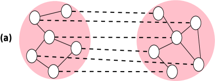
Figure 1: (a) Schematic diagram of a multiplex network consisting of two layers in which the solid lines represent intralayer couplings, whereas the dashed lines depict interlayer couplings. (b) Schematic diagram denoting evolution of networks using the genetic algorithm, where $G_{i}$ represents the $i^{th}$ network in a population. $G^{f}_{i}$ and $G^{c}_{i}$ represent $i^{th}$ fitter parent and child networks, respectively. The solid arrow represents progression of generation from the initial population and the dashed arrow indicates that the fitter and child graphs form the initial population for the next generation.

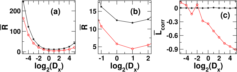
Figure 2: Minimized (circles) and initial (stars) average value of $R$ for various interlayer coupling strength in panel (a) and its zoomed version in panel (b). Panel (c) shows the values of the correlation $\overline{L}_{\mathrm{corr}}$ for initial ER random networks (stars) and optimized networks (circles). For each case, GA minimize the $R$ till 6000 iterations and the average is taken over population of 1000 networks and for the last 1000 iterations. Each initial layer of ER networks have $\langle k\rangle$=6 and $N=100$ [26].

Theoretical framework: We consider a bi-layer multiplex network, each layer having $P$ network population with a fixed size $N$ and a fixed average degree $\langle k\rangle$. The networks representing different layers may have different architecture. Let the adjacency matrix of the first and second layers be denoted by $A^{i}$ and $B^{i}$, respectively, where $1\leqslant i\leqslant P$. The weighted adjacency matrix $M^{i}$ of size 2N$\times$2N for the multiplex network (Fig. 1(a)) is defined by

$$M^{i}=\left[\begin{array}[]{cc}A^{i}~{}~{}D_{x}I\\ D_{x}I~{}~{}B^{i}\end{array}\right]$$ (1)

where I is the identity matrix of size N$\times$N and $D_{x}$ is the interlayer coupling strength.

Figure 3: Average value of $R_{norm}$ when individual network in a population is represented as (a) ER and (b) scale-free networks, respectively. For each case, GA minimizes the value of $R$ till 6000 iterations and the average is taken over the population of 1000 networks for last 1000 iterations. Each layer of the networks have $\langle k\rangle$=6 and $N=100$, which are preserved throughout the evolution.

The Laplacian matrix $L^{i}$ obtained from $M^{i}$ is defined by

$$L^{i}_{jk}=\begin{cases}~{}~{}~{}d^{i}_{j}~{}~{}~{}~{}\mbox{if }{~{}~{}~{}j\not=k}\\ -M^{i}_{jk}~{}~{}\mbox{otherwise},\end{cases}$$ (2)

where $d^{i}_{j}=\sum_{k}M^{i}_{jk}$. Let $\lambda^{i}_{1}$ $<$ $\lambda^{i}_{2}$ $\leqslant$ …. $\leqslant$ $\lambda^{i}_{2N}$ be the eigenvalues of $L^{i}$. The eigenvalue ratio $R^{i}$ = $\lambda^{i}_{2N}$/$\lambda^{i}_{2}$ of the $L^{i}$ matrix is used as a fitness function of $i^{th}$ multiplex network in the genetic algorithm. A network having the lesser $R$ value is more fit. Out of $P$ population of the initial networks, we select $P/2$ fitter networks for the next generation, which we term as the parent networks (Fig. 1(b)). The remaining $P/2$ networks of the next generation, known as the child networks, are constructed from the parent networks as follows. First a pair of the matrices is selected randomly from the $P/2$ population and then the adjacency matrices of these selected parent networks, termed as the parent matrices, are used to construct one crossed child matrix. Each block of this child matrix is constructed from the block having the same position in one of the parent matrices which are selected with the equal probability. Then, by taking the upper triangular part of the crossed matrix, a symmetric child matrix is built leading to the undirected child network. Further, the average degree of the crossed matrix is preserved by randomly inserting or deleting 1 and 0 entries decided by a probability. This probability is dependent on the fluctuations of $1$ entries from the adjacency matrices of the parent networks. The details of these steps are given in [23]. The process is repeated until we generate $P/2$ child networks which along with the $P/2$ parent networks form the same size of the population as of the initial networks. The networks are evolved until we attain the steady state. We measure various structural properties of networks as they evolve and analyze the interplay of these properties with the optimization of synchronizability.

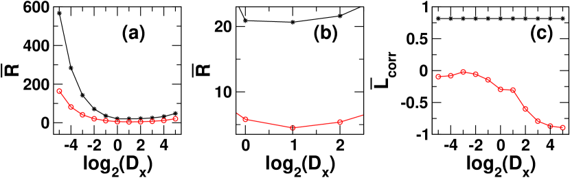
Figure 4: Minimized (circles) and initial (stars) average value of $R$ for various interlayer coupling strength in panel (a) and its zoomed version in panel (b). Panel (c) shows the values of the correlation $\overline{L}_{\mathrm{corr}}$ for initial SF networks (stars) and optimized networks (circles). For each case GA minimize the $R$ till 6000 iterations and the average of is taken over population of 1000 networks and last 1000 iterations. Each initial layer of scale-free networks have $\langle k\rangle$=6 and $N=100$.

Results and Discussion: In order to draw a close coherence with the real world networks, we consider the sparse networks as the initial population in GA. Starting with networks having random architecture, we evolve them using GA taking $R$ as the fitness function. We find that at the lower interlayer couplings ($D_{x}<<1$), the $\overline{R}$ is high which decreases with an increase in the $D_{x}$ values. At a certain $D_{x}$ value, the $\overline{R}$ attains its minima, then saturates followed by an increase in its value for $D_{x}>>1$ (Fig. 2(a),(b)). Note that for all the simulations, the size and the average degree of individual layer remains same as for the initial network, hence, any change in the value of $\overline{R}$ for initial network population is arising due to changes in the $D_{x}$ values. The lower $D_{x}$ values indicate the higher values of $R$ as at lower interlayer coupling strength the $\lambda_{2}$ values are low and at higher $D_{x}$ values the $\lambda_{N}$ values are high. Both the factors contribute to an increase in the $R$ values [16] and for the model considered in the Letter, $R$ can be determined as following: Case(1), when $D_{x}<<1$

$$R\approx\frac{\max\limits_{\alpha}\big{[}\lambda_{max}(L^{\alpha})~{}+~{}D_{x}\big{]}}{2D_{x}}$$ (3)

where $L^{\alpha}$ is the Laplacian of $\alpha^{th}$ layer, $\lambda_{max}(L^{\alpha})$ is the maximum eigenvalue of the Laplacian of $\alpha$th layer. Case(2), when $D_{x}>>$ 1

$$R\approx\frac{2D_{x}+\sqrt{2}\lambda_{max}(L^{AV})}{\lambda_{2}(L^{AV})}$$ (4)

where $L^{AV}$ is average Laplacian of two layers [16]. Eq. 3 indicates that $R$ is a decreasing function of $D_{x}$ for weaker interlayer coupling strength whereas Eq. 4 indicates that $R$ is an increasing function of $D_{x}$ for the stronger interlayer coupling strength. Consequently there is a trade off between both the behaviors leading to a value of $D_{x}$ for which $R$ achieves its minimum value. It turns out that this minimum value occurs at $D_{x}$ = 2 and hence Eq. 4 stands as a better approximation for $R$. What follows that the structural changes in the architecture of the optimized networks affect the second term in the numerator and the denominator which collectively contribute to minimization of the $R$ values.

Further, we define the efficiency of optimization as $R_{norm}=R_{opt}/R_{ini}$, where $R_{ini}$ and $R_{opt}$ are the eigenvalue ratio of the initial and the optimized networks, respectively. A lower value of $R_{norm}$ reflects a high efficiency of the synchronizability. For the ER random networks, initially with an increase in the $D_{x}$ values, $R_{norm}$ remains almost constant until the interlayer coupling strength reaches to 0.50 (Fig. 3(a)). However, the value of $R_{norm}$ being less than one implies that there is an optimization efficiency with respect to the initial population. Thereafter, it exhibits an abrupt decrease and attains a minimum value for $D_{x}$ = 2. Therefore, GA finds a variability in the efficiency of the optimization for various values of $D_{x}$. The value of $R_{norm}$ starts increasing after attaining the minimum value. The above results indicate that the enhancement in the first term of the numerator of Eq. 4, which is proportional to the interlayer coupling strength, might lead to a decrease in the efficiency of the optimization ($R_{norm})$. The GA, thus maximizes the synchronizability for various values of the interlayer coupling strength (Fig. 2(a), (b)) with $D_{x}=2$ leading to the most efficient structure.

In order to capture the structural features emerging in the best synchronizable networks, we define the Pearson product correlation ($L_{\mathrm{corr}}$) between the degrees of the mirror nodes in the pair of the layers as the evolution progresses as;

$$L_{\mathrm{corr}}=\frac{(\sum_{i}(k_{i}-\langle k\rangle)(\sum_{i}(K_{i}-\langle K\rangle)}{[(\sum_{i}(k_{i}-\langle k\rangle)^{2}(\sum_{i}(K_{i}-\langle K\rangle)^{2}]^{1/2}},$$

where $k_{i}$ and $K_{i}$ are the degrees of $i^{th}$ node in the first and the second layers, respectively. The terms $\langle k\rangle$ and $\langle K\rangle$ denote the average degrees of the first and the second layers, respectively. $\overline{L}_{\mathrm{corr}}$ is the average over the $L_{\mathrm{corr}}$ values of the population used in the GA. For lower values of $D_{x}$($<$ 0.5), the optimized networks do not reveal significant changes in $\overline{L}_{\mathrm{corr}}$ and remain close to zero, with small random fluctuations. With a further increase in $D_{x}$ values, the average correlation $\overline{L}_{\mathrm{corr}}$ decreases for the optimized networks (Fig. 2(c)). This can be considered to occur in order to minimize the value of maximal load over the interlayer links.

The reasons behind the emerging behavior of $\overline{L}_{\mathrm{corr}}$ might be explained as follows. When the higher degree nodes in one layer are connected with the higher degree nodes of the second layer and the interlayer coupling strength is high as well ($D_{x}$ $>$ 1), there is a very high load on the interlayer links, making it to become a dominant factor for affecting the synchronizability of the network [8]. Whereas, in a situation when the higher degrees in one layer are connected with the lower degree nodes in another layer, the value of the maximal load on the interlayer links becomes less, leading to a homogeneity of the loads on the interlayer links. In order to achieve this homogeneity, at higher values of $D_{x}$, the optimized networks exhibit negative values of $\overline{L}_{\mathrm{corr}}$. These results demonstrate an impact of the multiplexity on the maximization of the synchronizability as well as an impact of the weighted couplings on the evolved network architecture.

Further, in order to demonstrate the impact of structural properties of the initially selected networks population on the structural properties of the optimized networks, we present the results for the scale-free networks taken as the initial population. The scale-free networks are generated using Barabasi-Albert algorithm [24]. As observed for the ER networks, the GA approach successfully minimizes the $R$ values for various $D_{x}$ values for the scale-free networks as well. The value of $D_{x}$, for which $R$ takes a minimum value, also remains same (Fig. 4(a), (b)). The $L_{corr}$ value for the initial networks population is positive (Fig. 4(c)) since the mirror nodes in both the layers are associated with the same time in the growth algorithm, but the optimized networks exhibit negative $L_{corr}$ values as $D_{x}$ increases (Fig. 4(c)). The efficiency of optimization for scale-free networks taken as the initial population, captured through $R_{norm}$, also exhibits a behavior similar to the ER random networks (Fig. 3(b)) at the same interlayer coupling strength, though the values of $R_{norm}$ are lesser than those of ER random networks probably due to the higher values of $R$ for scale-free networks as compared to the ER random networks.

Figure 5: (a) Average values of $R_{norm}$ as a function of $D_{x}$. For each case GA minimize the $R_{norm}$ till 6000 iterations and the average of is taken over population of 1000 networks and last 1000 iterations. Panel (b) shows the convergence of average of $R_{norm}$ values over GA networks populations with generations(G) for $D_{x}$ = 1. For both cases $E_{y}$ = 4 and each initial layer of ER networks have $\langle k\rangle$=6 and $N=100$.

In order to analyze the impact of intralayer coupling strength on the global synchronizability, we introduce a parameter $E_{y}$. The new weighted adjacency matrix $M^{i}$ for the multiplex network can be defined as,

$$M^{i}=\left[\begin{array}[]{cc}A^{i}~{}~{}D_{x}I\\ D_{x}I~{}~{}E_{y}B^{i}\end{array}\right]$$ (5)

We consider one layer having intralayer coupling strength stronger than that of the other layer ($E_{y}=4$ in Eq. 5). With an initial increase in $D_{x}$, the values $R_{\mathrm{norm}}$ remains unaffected. After a certain value of $D_{x}$, $R_{\mathrm{norm}}$ decreases drastically and thereafter for a certain range of $D_{x}$ the rate of decrement becomes less. After attaining a minimum value, $R_{\mathrm{norm}}$ increases again (Fig. 5(a)). This behavior shares a close similarity to the one observed for $E_{y}$ = 1 (Eq. 3), the major difference being the shift in the minima of $R_{\mathrm{norm}}$ towards right, appearing at $D_{x}$ = 16. The probable reason behind this shift might be rescaling of the $D_{x}$ values with respect to $E_{y}$ towards the regime $D_{x}$ $<<$ 1. As a result, Eq. 3 holds good instead of Eq. 4 for the rescaled values of $D_{x}$ lying in the regime $D_{x}$ $<<$ 1.

Furthermore, there is a nearly similar behavior of convergence of $R_{norm}$ with an increase in generation (G) of the GA. We find that initially with an increase in the generation, the $\overline{R}_{norm}$ values exhibit a faster decrement (Fig. 5(b)). After a certain value of G, the $\overline{R}_{norm}$ converges to a fixed value and the properties affecting the optimization of the networks population saturate. This leads to a steady value of $\overline{R}_{norm}$ which remains unaffected by a further increase in G.

Figure 6: Average value of the variance of degree and betweenness centrality of the nodes in the optimized networks in the left and right panels, respectively. Initial layer of each ER network has $\langle k\rangle$=6 and $N=100$.

Further, to analyze the properties in the optimized networks, we calculate the variance in the degree and the betweenness centrality [25] for the different $D_{x}$ values. The initial ER random networks population has certain amount of degree heterogeneity due to the Poisson degree distribution [24]. For the lower interlayer coupling strength ($D_{x}<2$), the heterogeneity is suppressed (Fig.  6). With a further decrease in the $D_{x}$ values, the suppression in the degree heterogeneity remains invariant, beyond which the suppression decreases in the optimized networks (Fig.  6(a)). Note that there is a higher heterogeneity in the connectivity for $D_{x}$ = 2 as compared to $D_{x}$ = 1. Further, the betweenness centrality of a node can also be treated as a measure of the load distribution over the nodes in a network [12]. The ER random networks forming the initial population again display a certain amount of the betweenness centrality heterogeneity. For the higher coupling strength, the heterogeneity in betweenness centrality is not much suppressed in the optimized networks, however with a decrease in the interlayer coupling strength the suppression increases and converges to the homogeneous distribution at the lower coupling regime (Fig.  6(b)). Though the optimized networks suppress heterogeneity in the degree as well as in the betweenness centrality, the interlayer coupling strength plays an instrumental role in deciding the amount of heterogeneity. The larger interlayer coupling strengths lead to more heterogeneity in the various structural properties of the optimized networks.

These behaviors can be explained from the nature of Eq. 3 and Eq. 4. From Eq. 3, which holds good in the regime $D_{x}$ $>>$ 1, a structural change leads to a variation in the maxima of $\lambda_{max}$ over layers by keeping its denominator constant for a given $D_{x}$ value. Since the upper bound of $\lambda_{max}$ is an increasing function of the maximum degree of a network [27], a minimized value of $\lambda_{max}$ is achieved when the maxima of the degree of networks in both the layers are minimized. However in regime $D_{x}$ $>>$ 1, average value of $\lambda_{2}$ of the Laplacian for the layers appear in the denominator of Eq. 4 which is lower bounded by the inverse of the diameter of the network multiplied with the total number of connections [19], providing another degree of freedom. As a result sufficient amount of the homogeneity does not emerge in the optimized networks.

Conclusion: To conclude, we study the behavior of synchronizability in the multiplex networks with respect to interlayer coupling strength. Various bounds for $D_{x}$ provide an understanding to how interlayer coupling strength turns out to be a deciding factor for achieving the most synchronizable networks as well as for the efficiency of the optimization. The results presented here have two fold applications, one being the influence of the weights in coupling strength on the synchronizability and the other pertains to the importance of the multiplex network framework in capturing the enhancement in the synchronizability and the identification of the structural features whose interplay can help in designing the best synchronizable networks. The behavior of the synchronizability with respect to the interlayer coupling strength is robust against changes in the initial networks architecture. Based on the eigenvalue ratio, we argue that a particular interlayer coupling strength value leads to the highest efficiency of the optimization. Interestingly, the dynamical behavior of individual layers has been demonstrated to be largely affected while using them in the multiplex network framework. While the individual layers may not be favoring synchronizability, the evolved multiplex networks can be best synchronizable demonstrating the importance of multilayer framework. Additionally, the betweenness centrality of the edges being treated as the load distribution [12] explains the emergence of the negative correlation in the mirror nodes in the best synchronizable networks.

The framework and analysis presented here can be extended further in identifying a particular layer of the multiplex network which can be targeted to achieve the best or the worst synchronizable multiplex networks. Further, the approach presented in this Letter can be adopted to optimize other dynamical properties [28] in multiplex networks having restrictions on wiring topologies [29].

Acknowledgements: SJ thanks CSIR, Govt. of India project grant (25(0205)/12/EMR-II) and DST, Govt. of India project grant (EMR/2014/000368) for financial support. SKD acknowledges University Grants Commission, Govt. of India, for the fellowship.

References

- [1] J. Kurths, A. Pikovsky, and M. Rosenblum, Synchronization: A Universal Concept in Nonlinear Sciences (Cambridge University Press, Cambridge, 2001).
- [2] S. Boccaletti et. al., Physics Reports 424, 175 (2006).
- [3] A. Arenas et al., Physics Reports 469 93 (2008).
- [4] I. Belykh, E. de Lange, and M. Hasler, Phys. Rev. Lett. 94, 188101 (2005).
- [5] A. E. Motter et al., Phys. Rev. E 71, 016116 (2005).
- [6] M. Boguñà et al., Phys. Rev. Lett. 90, 028701 (2003).
- [7] J. G. Restrepo et al., Chaos 16, 015107 (2006).
- [8] T. Nishikawa et al., Phys. Rev. Lett. 91, 014101 (2003).
- [9] M. Barahona and L. M. Pecora, Phys. Rev. Lett. 89, 054101 (2002).
- [10] J. G. Restrepo, and E. Ott, and H. R. Brian, Phys. Rev. Lett. 96 254103 (2006).
- [11] L. M. Pecora and T. L. Carroll, Phys. Rev. Lett. 80, 2109 (1998).
- [12] L. Donetti, et al., Phys. Rev. Lett. 95, 188701 (2005).
- [13] S. Boccaletti, et al., Phys. Rep. 544, 1 (2014).
- [14] F. Battiston, V. Nicosia and V. Latora, Phys. Rev. E. 89, 032804 (2014)
- [15] S. Gómez, et al., Phys. Rev. Lett. 110, 028701 (2013)
- [16] A. Sole-Ribalta, et al., Phys. Rev. E 88 (2013).
- [17] S. H. Yook, H. Jeong, and A.-L. Barabási, Phys. Rev. Lett. 86 (25), 5835 (2001).
- [18] A. Barrat et al., PNAS 101 (11), 3747 (2004).
- [19] F. R. K. Chung, Spectral Graph Theory (American Mathematical Society, 1997).
- [20] F. Bauer, F. M. Atay, and J. Jost, EPL 89, 20002 (2010); F. M. Atay, J. Jost, and A. Wende, Phys. Rev. Lett. 92, 144101 (2004).
- [21] C. Zhou and J. Kurths, Phys. Rev. Lett. 96, 164102 (2006).
- [22] M. Chavez, et al., Phys. Rev. Lett. 94, 218701 (2005).
- [23] S.K. Dwivedi and S. Jalan, Phys. Rev. E. 90, 032803 (2014).
- [24] R. Albert and A.-L. Barabasi, Rev. Mod. Phys. 74, 47 (2002).
- [25] M. E. J. Newman, Networks: An Introduction (Oxford University Press, Oxford, 2010).
- [26] Note that with a change in the average degree of the networks, the value of for which the best synchronizable networks are obtained shifts, although the behavior of interlayer coupling strength remains same. Further, the interlayer coupling strength still is the deciding factor for the evolution of the heterogeneity in the degree and the betweenness centrality. For larger network size, requirement of the memory allocation for a population of networks in GA amounting to size of the 1-d array, becomes computationally very exhaustive. The network considered for the GA model in E. A. Variano et. al., Phys. Rev. Lett. 92, 188701 (2004) is 25.
- [27] K. Ch. Das, Linear Algebra Appl. 368 269 (2003).
- [28] G. Li et. al., Phys. Rev. E 87, 042810 (2013).
- [29] A. Halu, S. Mukharjee and G. Bianconi, Phys. Rev. E 89 012806 (2014).