Quadratic Convergence of Levenberg-Marquardt Method
for Elliptic and Parabolic Inverse Robin Problems

Abstract

We study the Levenberg-Marquardt (L-M) method for solving the highly nonlinear and ill-posed inverse problem of identifying the Robin coefficients in elliptic and parabolic systems. The L-M method transforms the Tikhonov regularized nonlinear non-convex minimizations into convex minimizations. And the quadratic convergence of the L-M method is rigorously established for the nonlinear elliptic and parabolic inverse problems for the first time, under a simple novel adaptive strategy for selecting regularization parameters during the L-M iteration. Then the surrogate functional approach is adopted to solve the strongly ill-conditioned convex minimizations, resulting in an explicit solution of the minimisation at each L-M iteration for both the elliptic and parabolic cases. Numerical experiments are provided to demonstrate the accuracy and efficiency of the methods.

Key Words. Inverse Robin problems, Levenberg-Marquardt method, surrogate functional.

1 Introduction

We are concerned in this work with the determination of the Robin coefficient in both stationary elliptic and time-dependent parabolic systems from noisy measurement data on a partial boundary. This is a highly nonlinear and ill-posed inverse problem and arises in many applications of practical importance. The Robin coefficient may characterize the thermal properties of conductive materials on the interface or certain physical processes near the boundary, e.g., it represents the corrosion damage profile in corrosion detection [5][7], and indicates the thermal property in quenching processes [15].

For the description of the model problems that are considered in this work, we let $\Omega\subset R^{d}~{}(d\geq 1)$ be an open bounded and connected domain, with a boundary $\partial\Omega$, which consists of two disjointed parts $\partial\Omega=\Gamma_{i}\cup\Gamma_{a}$, with $\Gamma_{i}$ and $\Gamma_{a}$ each being a $(d-1)$-dimensional polyhedral surface. $\Gamma_{i}$ and $\Gamma_{a}$ are respectively the part of the boundary that is inaccessible and accessible to experimental measurements. Then we shall consider the inverse Robin problems associated with the elliptic boundary value problem

$$\left\{\begin{array}[]{rclll}-\nabla\cdot(a({\bf x})\nabla u)+c({\bf x})u&=&f({\bf x})&\mbox{in}&\Omega\,,\\ a({\bf x})\frac{\partial u}{\partial n}+\gamma({\bf x})u&=&g({\bf x})&\mbox{on}&\Gamma_{i}\,,\\ a({\bf x})\frac{\partial u}{\partial n}&=&h({\bf x})&\mbox{on}&\Gamma_{a}\,,\end{array}\right.$$ (1.1)

and the parabolic initial boundary value problem

$$\left\{\begin{array}[]{rclll}\partial_{t}u-\nabla\cdot(a({\bf x})\nabla u)&=&f({\bf x},t)&\mbox{in}&\Omega\times[0,T]\,,\\ a({\bf x})\frac{\partial u}{\partial n}+\gamma({\bf x})u&=&g({\bf x},t)&\mbox{on}&\Gamma_{i}\times[0,T]\,,\\ a({\bf x})\frac{\partial u}{\partial n}&=&h({\bf x},t)&\mbox{on}&\Gamma_{a}\times[0,T]\,,\\ u({\bf x},0)&=&u_{0}({\bf x})&\mbox{in}&\Omega\,.\end{array}\right.$$ (1.2)

The coefficients $a({\bf x})$ and $c({\bf x})$ are the heat conductivity and radiation coefficient, satisfying that $\underline{a}\leq a({\bf x})\leq\bar{a}$ and $\underline{c}\leq c({\bf x})\leq\bar{c}$ in $\Omega$, where $\underline{a},\,\bar{a}$ and $\underline{c},\,\bar{c}$ are positive constants. Functions $f$, $g$ and $h$ are the source strength, ambient temperature and heat flux respectively. Both coefficients $\gamma({\bf x})$ in (1.1) and (1.2) represent the Robin coefficients, which will be the focus of our interest and is assumed to stay in the following feasible constraint set:

$$K:=\Big{\{}\gamma\in L^{2}(\Gamma_{i});\,\,0<\gamma_{1}\leq\gamma({\bf x})\leq\gamma_{2}\,\,a.e.\,\,{\rm on}\,\,\Gamma_{i}\Big{\}},$$

where $\gamma_{1}$ and $\gamma_{2}$ are two positive constants. For convenience, we often write the solutions of the systems (1.1) and (1.2) as $u(\gamma)$ to emphasize their dependence on the Robin coefficient $\gamma$.

We are now ready to formulate the inverse problems of our interest in this work.

Elliptic Inverse Robin Problem: recover the Robin coefficient $\gamma({\bf x})$ in (1.1) on the inaccessible part $\Gamma_{i}$ from the measurable data $z$ of $u$ on the accessible part $\Gamma_{a}$.

Parabolic inverse Robin problem: recover the Robin coefficient $\gamma({\bf x})$ in (1.2) on the inaccessible part $\Gamma_{i}$ from the measurable data $z$ of $u$ on the accessible part $\Gamma_{a}$ over the whole time range $[0,T]$.

The inverse Robin problems have been widely studied in literature; see [5] [2] [10][11][12] and the references therein. The Gauss-Newton method was applied in [5] to solve the least-squares formulation of the elliptic inverse Robin problem, but with no consideration of regularizations. An $L^{1}$-tracking functional approach was suggested for the elliptic inverse Robin problem in [2]. Effectiveness and justifications of least-squares formulations with regularizations were analysed in [10][11][12] for the Robin inverse problems, and some iterative methods were applied to solve the resulting nonlinear least-squares minimizations. However, we may observe a common feature of these existing methods, which solve directly the nonlinear optimizations resulting from least-squares formulations with regularisations, but these optimisation problems are highly non-convex as the forward solution $u(\gamma)$ is nonlinear with respect to $\gamma$, and strongly unstable at discrete level with fine mesh sizes and time step sizes due to the severe ill-posedness of the inverse problems and the fact that noise is always present in the observation data.

In order to alleviate the effects of these drawbacks, we shall apply the L-M iterative method [4] [6] [13] [14] [16] to solve the nonlinear optimizations resulting from least-squares formulations with regularisations for the concerned inverse Robin problems. With the L-M method, we need only to solve a convex optimization at each iteration. Furthermore, in combination with the surrogate functional technique, we will not require the solution of any optimisation problems in each iteration as the minimisers can be computed explicitly. Another important novelty of this work is its establishment of the quadratic rate of convergence of the L-M method for both the elliptic and parabolic inverse Robin problems. This appears to be the first time in literature to demonstrate the quadratic convergence of the L-M method for a highly nonlinear ill-posed inverse problem. Compared with general optimal control problems or general direct nonlinear optimisation systems, the analysis on the quadratic rate of convergence of the L-M method here is much more delicate and tricky, due to the severe ill-posedness, high nonlinearity and strong instability of the current inverse problems and the direct effect on the convergence from two crucial parameters involved, namely the regularization parameter and the noise level in the data.

The rest of the paper is organized as follows. In Section 2, we discuss the uniqueness of the nonlinear elliptic and parabolic inverse Robin problems. In Sections 3 and 4, we formulate the Tikhonov regularizations for the nonlinear elliptic and parabolic inverse Robin problem respectively and study some mathematical properties of the resulting nonlinear optimisations. In Subsections 3.1 and 4.1, Fréchet derivatives of the forward solution of (1.1) and (1.2) and corresponding adjoint operators are derived respectively. In Subsections 3.2 and 4.2, the L-M iterative methods are formulated and their quadratic convergences are established. The surrogate functional approach is applied in Subsections 3.3 and 4.3 to solve the convex minimization at each L-M iteration for the nonlinear elliptic and parabolic inverse Robin problem respectively. Several numerical experiments are presented in Section 5 to illustrate the efficiency and accuracy of the proposed methods. Some concluding remarks are given in Section 6.

Throughout this work, $C$ is often used for a generic positive constant. We shall use the symbol $\langle\cdot,\cdot\rangle$ for the general inner product, and write the norms of the spaces $H^{m}(\Omega)$, $L^{2}(\Omega)$, $H^{{1}/{2}}(\Gamma)$ and $L^{2}(\Gamma)$ (for some $\Gamma\subset\partial\Omega$) respectively as $\|\cdot\|_{m,\Omega}$, $\|\cdot\|_{\Omega}$, $\|\cdot\|_{1/2,\Gamma}$ and $\|\cdot\|_{\Gamma}$.

2 Uniqueness and local Lipschitz stability of the inverse Robin problems

In this section, we shall demonstrate the uniqueness and local Lipschitz stability of the Robin coefficients in the concerned nonlinear elliptic and parabolic inverse Robin problems.

We first study the uniqueness and local Lipschitz stability of the elliptic inverse Robin problem.

Theorem 2.1.

(Uniqueness of the elliptic inverse Robin problem) Let $\gamma_{1}$ and $\gamma_{2}$ be two solutions to the elliptic inverse Robin problem as stated in Section 1, and $\partial\Omega$ be $C^{2}$ smooth. Furthermore, we assume that ${\rm meas}(\{{\bf x}\in\Gamma_{i};\,u({\bf x})=0\})=0$ where $u$ is the solution to the forward system (1.1), then $\gamma_{1}=\gamma_{2}$ almost everywhere on $\Gamma_{i}$.

Proof. It is straightforward to verify using (1.1) that $u(\gamma_{1})-u(\gamma_{2})$ satisfies

$$\left\{\begin{array}[]{rclll}-\nabla\cdot(a({\bf x})\nabla(u(\gamma_{1})-u(\gamma_{2})))+c({\bf x})(u(\gamma_{1})-u(\gamma_{2}))&=&0&\mbox{in}&\Omega\,,\\ a({\bf x})\frac{\partial(u(\gamma_{1})-u(\gamma_{2}))}{\partial n}&=&0&\mbox{on}&\Gamma_{a}\,,\\ u(\gamma_{1})-u(\gamma_{2})&=&0&\mbox{on}&\Gamma_{a}\,,\end{array}\right.$$ (2.4)

and on the boundary $\Gamma_{i}$,

$$a({\bf x})\frac{\partial(u(\gamma_{1})-u(\gamma_{2}))}{\partial n}+\gamma_{1}u(\gamma_{1})-\gamma_{2}u(\gamma_{2})=0.$$ (2.5)

The unique continuation principle [8] implies that $u(\gamma_{1})-u(\gamma_{2})=0$ in $\Omega$. Hence, by the trace theorem and the weak form of the system (2.4), we have

$$\|u(\gamma_{1})-u(\gamma_{2})\|_{\partial\Omega}\leq C\|u(\gamma_{1})-u(\gamma_{2})\|_{1,\Omega}=0,$$

and for any $\varphi\in H^{1}(\Omega)$,

$$\int_{\Gamma_{i}}a({\bf x})\frac{\partial(u(\gamma_{1})-u(\gamma_{2}))}{\partial n}\varphi ds=\int_{\Omega}a({\bf x})\nabla(u(\gamma_{1})-u(\gamma_{2}))\cdot\nabla\varphi+c({\bf x})(u(\gamma_{1})-u(\gamma_{2}))\varphi d{\bf x}=0\,.$$

Therefore we immediately see sthat

$$a({\bf x})\frac{\partial(u(\gamma_{1})-u(\gamma_{2}))}{\partial n}=0~{}~{}~{}~{}{\rm and}~{}~{}~{}~{}u(\gamma_{1})=u(\gamma_{2})~{}~{}~{}~{}{\rm on}~{}~{}~{}~{}\Gamma_{i},$$

which, along with (2.5), leads to

$$u(\gamma_{1})(\gamma_{1}-\gamma_{2})=0~{}~{}~{}~{}{\rm on}~{}~{}~{}~{}\Gamma_{i}.$$

Now the assumption that ${\rm meas}(\{{\bf x}\in\Gamma_{i}:\,u({\bf x})=0\})=0$ implies $\gamma_{1}=\gamma_{2}$ a.e. on $\Gamma_{i}$. $\sharp$

For the local Lipschitz stability, let $\gamma^{*}$ be the true Robin coefficient, we shall write for any positive constant $b$ that

$$N(\gamma^{*},b)=\{\gamma\in K;\,\,\|\gamma-\gamma^{*}\|_{\Gamma_{i}}\leq b\}.$$ (2.6)

Then we refer to [9] and give the following theorem to show the local Lipschitz stability.

Theorem 2.2.

(Local Lipschitz stability of the elliptic inverse Robin problem) Assume that $u(\gamma^{*})\geq c_{0}>0$ on $\Gamma_{i}$, then there exists a positive constant $b$ such that the following stability estimate holds:

$$\|u(\gamma_{1})-u(\gamma_{2})\|_{\Gamma_{a}}\geq C\|\gamma_{1}-\gamma_{2}\|_{\Gamma_{i}}\quad\forall\,\gamma_{1},\gamma_{2}\in N(\gamma^{*},b)\,.$$ (2.7)

Next, we study the uniqueness and local Lipschitz stability of the parabolic inverse Robin problem.

Theorem 2.3.

(Uniqueness of the parabolic inverse Robin problems) Let $\gamma_{1}$ and $\gamma_{2}$ be two solutions to the parabolic inverse Robin problem as stated in Section 1, and $\partial\Omega$ be $C^{2}$ smooth. Moreover, we assume that ${\rm meas}(\{{\bf x}\in\Gamma_{i};\,u({\bf x},t)=0~{}\mbox{for}~{}t\in(0,T)\})=0$, where $u$ is the solution to the forward system (1.2), then $\gamma_{1}=\gamma_{2}$ almost everywhere on $\Gamma_{i}$.

Proof. It is straightforward to verify using (1.2) that $u(\gamma_{1})-u(\gamma_{2})$ satisfies

$$\left\{\begin{array}[]{rclll}\partial_{t}(u(\gamma_{1})-u(\gamma_{2}))-\nabla\cdot(a({\bf x})\nabla(u(\gamma_{1})-u(\gamma_{2})))&=&0&\mbox{in}&\Omega\times[0,T]\,,\\ a({\bf x})\frac{\partial(u(\gamma_{1})-u(\gamma_{2}))}{\partial n}&=&0&\mbox{on}&\Gamma_{a}\times[0,T]\,,\\ u(\gamma_{1})-u(\gamma_{2})&=&0&\mbox{on}&\Gamma_{a}\times[0,T]\,,\\ (u(\gamma_{1})-u(\gamma_{2}))({\bf x},0)&=&0&\mbox{in}&\Omega\,,\end{array}\right.$$ (2.12)

and on the boundary $\Gamma_{i}\times[0,T]$,

$$a({\bf x})\frac{\partial(u(\gamma_{1})-u(\gamma_{2}))}{\partial n}+\gamma_{1}u(\gamma_{1})-\gamma_{2}u(\gamma_{2})=0.$$ (2.13)

The unique continuation principle [8] implies that $u(\gamma_{1})-u(\gamma_{2})=0$ in $\Omega\times[0,T]$. Hence, by the trace theorem and the weak form of the system (2.12), we have

$$\|u(\gamma_{1})-u(\gamma_{2})\|_{\partial\Omega}\leq C\|u(\gamma_{1})-u(\gamma_{2})\|_{1,\Omega}=0,$$

and for any $\varphi\in L^{2}(0,T;H^{1}(\Omega))$,

$$\int_{0}^{T}\int_{\Gamma_{i}}a({\bf x})\frac{\partial(u(\gamma_{1})-u(\gamma_{2}))}{\partial n}\varphi dsdt = \int_{0}^{T}\int_{\Omega}a({\bf x})\nabla(u(\gamma_{1})-u(\gamma_{2}))\cdot\nabla\varphi d{\bf x}dt$$

$$+\int_{0}^{T}\int_{\Omega}\partial_{t}(u(\gamma_{1})-u(\gamma_{2}))\varphi d{\bf x}dt=0\,.$$

Therefore we immediately see that

$$a({\bf x})\frac{\partial(u(\gamma_{1})-u(\gamma_{2}))}{\partial n}=0~{}~{}~{}~{}{\rm and}~{}~{}~{}~{}u(\gamma_{1})=u(\gamma_{2})~{}~{}~{}~{}{\rm on}~{}~{}~{}~{}\Gamma_{i}\times[0,T],$$

which, along with (2.13), yields sthat

$$u(\gamma_{1})(\gamma_{1}-\gamma_{2})=0~{}~{}~{}~{}{\rm on}~{}~{}~{}~{}\Gamma_{i}\times[0,T].$$

Now the assumption ${\rm meas}(\{{\bf x}\in\Gamma_{i};\,u({\bf x},t)=0~{}{\rm for}~{}t\in(0,T)\})=0$ implies $\gamma_{1}=\gamma_{2}$ a.e. on $\Gamma_{i}$. $\sharp$

For the local Lipschitz stability, we also refer to [9] and give the following theorem to show the local Lipschitz stability.

Theorem 2.4.

(Local Lipschitz stability of the parabolic inverse Robin problem) Assume that $u(\gamma^{*})\geq c_{0}>0$ on $\Gamma_{i}\times[0,T]$, then there exists a constant $b>0$ such that

$$\|u(\gamma_{1})-u(\gamma_{2})\|_{L^{2}(0,T;L^{2}(\Gamma_{a}))}\geq C\|\gamma_{1}-\gamma_{2}\|_{\Gamma_{i}}\,\quad\forall\,\gamma_{1},\gamma_{2}\in N(\gamma^{*},b)\,.$$ (2.14)

3 Elliptic inverse Robin problem and its L-M solution

3.1 Tikhonov regularization for elliptic inverse Robin problem

In this section we first formulate the Levenberg-Marquardt method for solving the nonlinear non-convex optimisation problems resulting from the least-squares formulation of the elliptic inverse Robin problem as stated in Section 1, incorporated with Tikhonov regularization to handle its ill-posedness and instability due to the presence of the noise in the observation data [12]. We assume the noise level in the observation data $z^{\delta}$ of the true solution $u$ to the elliptic system (1.1) is of order $\delta$, namely

$$\|u(\gamma^{*})-z^{\delta}\|_{\Gamma_{a}}\leq\delta\,,$$ (3.1)

where $\gamma^{*}$ is the true Robin coefficient. The elliptic inverse Robin problem is frequently transformed into the following stabilized minimization system with Tikhonov regularization:

$$\min_{\gamma\in K}{\cal J}(\gamma) = \|u(\gamma)-z^{\delta}\|_{\Gamma_{a}}^{2}+\beta\|\gamma\|_{\Gamma_{i}}^{2}\,,$$ (3.2)

where $\beta$ is the regularization parameter. The formulation (3.2) was shown to be stable in the sense that its minimizer depends continuously on the change of the noise in the data $z^{\delta}$ [12].

For the subsequent analysis on the convergence of the Levenberg-Marquardt method for solving the optimisation (3.2), we shall frequently need the Fréchet derivative of the forward solution $u(\gamma)$ of system (1.1). Let $w:=u^{\prime}(\gamma)d$ be the Fréchet derivative at direction $d$, then it solves the following system:

$$\left\{\begin{array}[]{rccll}-\nabla\cdot(a({\bf x})\nabla w)+c({\bf x})w&=&0&\mbox{in}&\Omega\,,\\ a({\bf x})\frac{\partial w}{\partial n}+\gamma\,w&=&-d\,u(\gamma)&\mbox{on}&\Gamma_{i}\,,\\ a({\bf x})\frac{\partial w}{\partial n}&=&0&\mbox{on}&\Gamma_{a}\,.\end{array}\right.$$ (3.3)

Let $u^{\prime}(\gamma)^{*}$ be the adjoint operator of the Fréchet derivative $u^{\prime}(\gamma)$, then it it easy to verify that $w^{*}:=u^{\prime}(\gamma)^{*}p\in H^{1}(\Omega)$ at a general direction $p$ solves the following system

$$\left\{\begin{array}[]{rccll}-\nabla\cdot(a({\bf x})\nabla w^{*})+c({\bf x})w^{*}&=&0&\mbox{in}&\Omega\,,\\ a({\bf x})\frac{\partial w^{*}}{\partial n}+\gamma\,w^{*}&=&0&\mbox{on}&\Gamma_{i}\,,\\ a({\bf x})\frac{\partial w^{*}}{\partial n}&=&-p\,u(\gamma)&\mbox{on}&\Gamma_{a}\,.\end{array}\right.$$ (3.4)

The following lemma gives an important relation for our later study.

Lemma 3.1.

The following relation holds for any directions $d$ and $p$:

$$\langle w,\,u(\gamma)p\rangle_{\Gamma_{a}}=\langle u(\gamma)d,\,w^{*}\rangle_{\Gamma_{i}}.$$ (3.5)

Proof. For any $\varphi,\psi\in H^{1}(\Omega)$, we can readily derive the variational forms of systems (3.3) and (3.4):

$$\int_{\Omega}a({\bf x})\nabla w\cdot\nabla\varphi d{\bf x}+\int_{\Omega}c({\bf x})w\varphi d{\bf x}=\int_{\Gamma_{i}}(-du(\gamma)-\gamma w)\varphi ds,$$ (3.6)

$$\int_{\Omega}a({\bf x})\nabla w^{*}\cdot\nabla\psi d{\bf x}+\int_{\Omega}c({\bf x})w^{*}\psi d{\bf x}=-\int_{\Gamma_{i}}\gamma w^{*}\psi ds-\int_{\Gamma_{a}}pu(\gamma)\psi ds.$$ (3.7)

Now (3.5) follows by taking $\varphi=w^{*}$ and $\psi=w$ respectively in (3.6) and (3.7). $\sharp$

3.2 Levenberg-Marquardt method and its convergence

The nonlinearity of the forward solution $u(\gamma)$ of the system (1.1) makes the minimization (3.2) highly nonlinear and non-convex with respect to the Robin coefficient $\gamma$, as well as strongly unstable at discrete level with fine mesh sizes and time step sizes due to the severe ill-posedness of the inverse problem and the fact that noise is always present in the observation data. To alleviate these difficulties in numerical solutions, we shall apply the Levenberg-Marquardt method to solve (3.2). For a given $\bar{\gamma}\in K$, we apply the linearization

$$u(\gamma)\approx u(\bar{\gamma})+u^{\prime}(\bar{\gamma})(\gamma-\bar{\gamma}),$$

then we may solve the minimization system (3.2) by the following Levenberg-Marquardt iteration, which is widely used for general nonlinear optimization problems [4] [16]:

$$J(\gamma^{k+1})=\min_{\gamma\in K}J(\gamma):=\|u^{\prime}(\gamma^{k})(\gamma-\gamma^{k})-(z^{\delta}-u(\gamma^{k}))\|_{\Gamma_{a}}^{2}+\beta_{k}\|\gamma-\gamma^{k}\|_{\Gamma_{i}}^{2}\,.$$ (3.8)

Before our study of the convergence of the iteration (3.8), we shall develop some auxiliary results.

Lemma 3.2.

Assume the forward operator $u(\gamma)$ of system (1.1) satisfies that $u(\gamma)\in L^{\infty}(\Gamma_{i})$ for $\gamma\in K$, then there exist two positive constants $L$ and $c_{1}$ such that the following estimates hold for all $\gamma,\,\bar{\gamma}\in K$:

$$\|u(\gamma)-u(\bar{\gamma})\|_{\Gamma_{a}} \leq L\|\gamma-\bar{\gamma}\|_{\Gamma_{i}},$$ (3.9)

$$\|u^{\prime}(\bar{\gamma})(\gamma-\bar{\gamma})-(u(\gamma)-u(\bar{\gamma}))\|_{\Gamma_{a}} \leq c_{1}\|\gamma-\bar{\gamma}\|^{2}_{\Gamma_{i}}\,.$$ (3.10)

Proof. From the variational form of the system (1.1), we can easily find that

$$\int_{\Omega}a({\bf x})\nabla(u(\gamma)-u(\bar{\gamma}))\cdot\nabla\varphi d{\bf x}+\int_{\Omega}c({\bf x})(u(\gamma)-u(\bar{\gamma}))\varphi d{\bf x}$$ (3.11)

$$+ \int_{\Gamma_{i}}\bar{\gamma}(u(\gamma)-u(\bar{\gamma}))\varphi ds=-\int_{\Gamma_{i}}(\gamma-\bar{\gamma})u(\gamma)\varphi ds.$$

Taking $\varphi=u(\gamma)-u(\bar{\gamma})$ and using the lower bounds of $a({\bf x})$, $c({\bf x})$, and $\bar{\gamma}$, we derive

$$\min\{\underline{a},\underline{c}\}\|u(\gamma)-u(\bar{\gamma})\|^{2}_{1,\Omega}+\gamma_{1}\|u(\gamma)-u(\bar{\gamma})\|^{2}_{\Gamma_{i}}\leq|\int_{\Gamma_{i}}(\gamma-\bar{\gamma})u(\gamma)(u(\gamma)-u(\bar{\gamma}))ds|$$

$$\leq \|u(\gamma)\|_{L^{\infty}(\Gamma_{i})}\|\gamma-\bar{\gamma}\|_{\Gamma_{i}}\|u(\gamma)-u(\bar{\gamma})\|_{\Gamma_{i}}\leq C\|\gamma-\bar{\gamma}\|_{\Gamma_{i}}\|u(\gamma)-u(\bar{\gamma})\|_{\Gamma_{i}}.$$

Then it follows by the Cauchy-Schwarz inequality that

$$\min\{\underline{a},\underline{c}\}\|u(\gamma)-u(\bar{\gamma})\|^{2}_{1,\Omega}\leq\frac{C^{2}}{2\gamma_{1}}\|\gamma-\bar{\gamma}\|^{2}_{\Gamma_{i}}\,.$$

Now estimate (3.9) follows directly from this inequality and the trace theorem. To verify the estimate (3.10), we first show

$$\|u^{\prime}(\gamma)d\|_{\partial\Omega}\leq C\|d\|_{\Gamma_{i}}.$$ (3.12)

Indeed, choosing $\varphi=u^{\prime}(\gamma)d$ in (3.6), we readily get

$$\int_{\Omega}a({\bf x})|\nabla(u^{\prime}(\gamma)d)|^{2}d{\bf x}+\int_{\Omega}c({\bf x})|u^{\prime}(\gamma)d|^{2}d{\bf x}+\int_{\Gamma_{i}}\gamma|u^{\prime}(\gamma)d|^{2}ds=-\int_{\Gamma_{i}}du(\gamma)(u^{\prime}(\gamma)d)ds.$$

Then it follows by the Cauchy-Schwarz inequality that

$$\min\{\underline{a},\underline{c}\}\|u^{\prime}(\gamma)d\|^{2}_{1,\Omega}\leq\frac{C^{2}}{2\gamma_{1}}\|d\|^{2}_{\Gamma_{i}},$$

which, along with the trace theorem, gives (3.12) immediately.

Next, we prove the estimate (3.10). Taking $\gamma=\bar{\gamma}$ and $d=\gamma-\bar{\gamma}$ in (3.6), we have

$$\int_{\Omega}a({\bf x})\nabla u^{\prime}(\bar{\gamma})(\gamma-\bar{\gamma})\cdot\nabla\varphi d{\bf x}+\int_{\Omega}c({\bf x})u^{\prime}(\bar{\gamma})(\gamma-\bar{\gamma})\varphi d{\bf x}$$ (3.13)

$$+ \int_{\Gamma_{i}}\bar{\gamma}u^{\prime}(\bar{\gamma})(\gamma-\bar{\gamma})\varphi ds=-\int_{\Gamma_{i}}(\gamma-\bar{\gamma})u(\bar{\gamma})\varphi ds~{}~{}\forall\,\varphi\in H^{1}(\Omega)\,.$$

Subtracting (3.13) from (3.11) yields

$$\int_{\Omega}a({\bf x})\nabla(u^{\prime}(\bar{\gamma})(\gamma-\bar{\gamma})-(u(\gamma)-u(\bar{\gamma})))\cdot\nabla\varphi d{\bf x}+\int_{\Gamma_{i}}\bar{\gamma}(u^{\prime}(\bar{\gamma})(\gamma-\bar{\gamma})-(u(\gamma)-u(\bar{\gamma})))\varphi ds$$

$$+ \int_{\Omega}c({\bf x})(u^{\prime}(\bar{\gamma})(\gamma-\bar{\gamma})-(u(\gamma)-u(\bar{\gamma})))\varphi d{\bf x}=\int_{\Gamma_{i}}(\gamma-\bar{\gamma})(u(\gamma)-u(\bar{\gamma}))\varphi ds.$$

Then applying the trace theorem, Lagrange mean value theorem and inequality (3.12), we derive

$$\|u^{\prime}(\bar{\gamma})(\gamma-\bar{\gamma})-(u(\gamma)-u(\bar{\gamma}))\|_{\Gamma_{a}}\leq C\|u^{\prime}(\bar{\gamma})(\gamma-\bar{\gamma})-(u(\gamma)-u(\bar{\gamma}))\|_{1,\Omega}$$

$$\leq C\|(\gamma-\bar{\gamma})(u(\gamma)-u(\bar{\gamma}))\|_{\Gamma_{i}}=C\|(\gamma-\bar{\gamma})u^{\prime}(\xi)(\gamma-\bar{\gamma})\|_{\Gamma_{i}}\leq c_{1}\|\gamma-\bar{\gamma}\|^{2}_{\Gamma_{i}},$$

where $\xi$ is some element in $K$ between $\gamma$ and $\bar{\gamma}$. $\sharp$

Now we are ready to establish a quadratic rate on the convergence of the Levenberg-Marquardt method (3.8), under the following basic condition:

$$\|u(\gamma)-u(\gamma^{*})\|_{\Gamma_{a}}\geq c_{2}\|\gamma-\gamma^{*}\|_{\Gamma_{i}}\quad\forall\,\gamma\in N(\gamma^{*},b)$$ (3.14)

where $c_{2}$ and $b$ are two positive constants with $b\in(0,1)$. Here $N(\gamma^{*},b)$ denotes the $b$-neighborhood of the true Robin coefficient $\gamma^{*}\in K$ defined in (2.6). Assumption (3.14) is the frequently adopted basic condition to ensure the quadratic convergence of the Levenberg-Marquardt method for most direct nonlinear optimization problems [4] [16], so it is natural to bring it to the current nonlinear ill-posed inverse problems. The condition (3.14) may be viewed as a direct motivation of the local Lipschitz stability of the elliptic inverse Robin problems (see estimate (2.7) in Theorem 2.2).

It is a well-known technical difficulty in a practical numerical realisation of any Tikhonov regularised optimisation system like the ones (3.2) and (3.8) to choose a reasonable and effective regularization parameter $\beta$ or $\beta_{k}$. Another important novelty of this work is our suggestion of a very simple and easy implementable choice of the parameter $\beta_{k}$ based on the following rule:

$$\beta_{k}=\|u(\gamma^{k})-z^{\delta}\|^{2}_{\Gamma_{a}}\,.$$ (3.15)

And surprisingly, as we shall demonstrate below, this choice of the regularization parameter $\beta_{k}$ ensures a quadratical convergence of the resulting Levenberg-Marquardt iteration (3.8).

Considering the presence of the noise (see (3.1)), it is reasonable for us to terminate the L-M iteration (3.8) when its minimizer $\gamma^{k}$ is accurate enough in terms of the noise level, more specifically, we shall terminate the iteration if the following criterion is realised:

$$c_{2}\|\gamma^{k}-\gamma^{*}\|_{\Gamma_{i}}<2\delta\quad\mbox{or}\quad\|u(\gamma^{k})-z^{\delta}\|_{\Gamma_{a}}<\sqrt{\delta}\,.$$ (3.16)

Lemma 3.3.

Under the conditions (3.14), (3.15) and (3.16), if $\gamma^{k}\in N(\gamma^{*},b)$ then $\gamma^{k+1}$ generated by the iteration (3.8) satisfies

$$\|u^{\prime}(\gamma^{k})(\gamma^{k+1}-\gamma^{k})-(z^{\delta}-u(\gamma^{k}))\|_{\Gamma_{a}} \leq c_{3}(\|\gamma^{k}-\gamma^{*}\|^{2}_{\Gamma_{i}}+\delta),$$ (3.17)

$$\|\gamma^{k+1}-\gamma^{k}\|^{2}_{\Gamma_{i}} \leq c_{4}(\|\gamma^{k}-\gamma^{*}\|^{2}_{\Gamma_{i}}+\delta),$$ (3.18)

where constants $c_{3}$ and $c_{4}$ are given explicitly by $c_{3}=\sqrt{\max\{2c_{1}^{2}+2L^{2}+1,\,3\}}$ and $c_{4}=\max\{\frac{8c_{1}^{2}}{c_{2}^{2}}+1,\,2\}$.

Proof. As $\gamma^{k+1}$ is a minimizer in (3.8), we derive using the estimates (3.1), (3.9)-(3.10), equality (3.15) and the Cauchy-Schwarz inequality

$$\|u^{\prime}(\gamma^{k})(\gamma^{k+1}-\gamma^{k})-(z^{\delta}-u(\gamma^{k}))\|_{\Gamma_{a}}^{2}\leq J(\gamma^{k+1})\leq J(\gamma^{*})$$

$$= \|u^{\prime}(\gamma^{k})(\gamma^{*}-\gamma^{k})-(u(\gamma^{*})-u(\gamma^{k}))+u(\gamma^{*})-z^{\delta}\|_{\Gamma_{a}}^{2}+\beta_{k}\|\gamma^{*}-\gamma^{k}\|_{\Gamma_{i}}^{2}$$

$$\leq 2c_{1}^{2}\|\gamma^{k}-\gamma^{*}\|^{4}_{\Gamma_{i}}+2\delta^{2}+\|u(\gamma^{k})-u(\gamma^{*})+u(\gamma^{*})-z^{\delta}\|^{2}_{\Gamma_{a}}\|\gamma^{*}-\gamma^{k}\|_{\Gamma_{i}}^{2}$$

$$\leq 2c_{1}^{2}\|\gamma^{k}-\gamma^{*}\|^{4}_{\Gamma_{i}}+2\delta^{2}+2L^{2}\|\gamma^{*}-\gamma^{k}\|_{\Gamma_{i}}^{4}+2\delta^{2}\|\gamma^{*}-\gamma^{k}\|_{\Gamma_{i}}^{2}$$

$$\leq (2c_{1}^{2}+2L^{2}+1)\|\gamma^{k}-\gamma^{*}\|^{4}_{\Gamma_{i}}+(2+\delta^{2})\delta^{2}$$

$$\leq \max\{2c_{1}^{2}+2L^{2}+1,\,3\}(\|\gamma^{k}-\gamma^{*}\|^{4}_{\Gamma_{i}}+\delta^{2}),$$

which implies (3.17) immediately.

Again, using the minimizing property of $\gamma^{k+1}$ in (3.8) and the estimates (3.1) and (3.10), we can deduce as follows:

$$\|\gamma^{k+1}-\gamma^{k}\|^{2}_{\Gamma_{i}}\leq\frac{1}{\beta_{k}}J(\gamma^{k+1})\leq\frac{1}{\beta_{k}}J(\gamma^{*})$$ (3.19)

$$= \frac{1}{\beta_{k}}\|u^{\prime}(\gamma^{k})(\gamma^{*}-\gamma^{k})-(z^{\delta}-u(\gamma^{k}))\|_{\Gamma_{a}}^{2}+\|\gamma^{*}-\gamma^{k}\|_{\Gamma_{i}}^{2}$$

$$\leq \frac{1}{\beta_{k}}(2c_{1}^{2}\|\gamma^{k}-\gamma^{*}\|^{4}_{\Gamma_{i}}+2\delta^{2})+\|\gamma^{*}-\gamma^{k}\|_{\Gamma_{i}}^{2}$$

$$= \frac{2c_{1}^{2}\|\gamma^{k}-\gamma^{*}\|^{4}_{\Gamma_{i}}}{\|u(\gamma^{k})-z^{\delta}\|^{2}_{\Gamma_{a}}}+\frac{2\delta^{2}}{\|u(\gamma^{k})-z^{\delta}\|^{2}_{\Gamma_{a}}}+\|\gamma^{*}-\gamma^{k}\|_{\Gamma_{i}}^{2}.$$

As stated in (3.16), the iterative process (3.8) terminates if $c_{2}\|\gamma^{k}-\gamma^{*}\|_{\Gamma_{i}}<2\delta$ or $\|u(\gamma^{k})-z^{\delta}\|_{\Gamma_{a}}<\sqrt{\delta}$. Otherwise we have $c_{2}\|\gamma^{k}-\gamma^{*}\|_{\Gamma_{i}}\geq 2\delta$ and $\|u(\gamma^{k})-z^{\delta}\|_{\Gamma_{a}}\geq\sqrt{\delta}$. Then we can easily see that $\frac{2\delta^{2}}{\|u(\gamma^{k})-z^{\delta}\|^{2}_{\Gamma_{a}}}\leq 2\delta$ and

$$\|u(\gamma^{k})-z^{\delta}\|_{\Gamma_{a}}\geq\|u(\gamma^{k})-u(\gamma^{*})\|_{\Gamma_{a}}-\|u(\gamma^{*})-z^{\delta}\|_{\Gamma_{a}}$$

$$\geq c_{2}\|\gamma^{k}-\gamma^{*}\|_{\Gamma_{i}}-\delta\geq c_{2}\|\gamma^{k}-\gamma^{*}\|_{\Gamma_{i}}-\frac{c_{2}}{2}\|\gamma^{k}-\gamma^{*}\|_{\Gamma_{i}}=\frac{c_{2}}{2}\|\gamma^{k}-\gamma^{*}\|_{\Gamma_{i}}\,.$$

Now the desired result (3.18) follows readily from these two estimates and (3.19). $\sharp$

Lemma 3.4.

Under the conditions (3.14), (3.15) and (3.16), let $\gamma^{k}$ and $\gamma^{k+1}$ be two consequent iterates generated by the iteration (3.8) such that both $\gamma^{k}$ and $\gamma^{k+1}$ lie in $N(\gamma^{*},b)$, then

$$\|\gamma^{k+1}-\gamma^{*}\|_{\Gamma_{i}}\leq c_{5}(\|\gamma^{k}-\gamma^{*}\|^{2}_{\Gamma_{i}}+\delta),$$ (3.20)

where constant $c_{5}$ is given explicitly by $c_{5}={(c_{3}+c_{1}c_{4}+1)}/{c_{2}}$.

Proof. It follows from (3.14), (3.10), (3.17) and (3.18) that

$$c_{2}\|\gamma^{k+1}-\gamma^{*}\|_{\Gamma_{i}}\leq\|u(\gamma^{k+1})-u(\gamma^{*})\|_{\Gamma_{a}}\leq\|u(\gamma^{k+1})-z^{\delta}\|_{\Gamma_{a}}+\delta$$

$$= \|u^{\prime}(\gamma^{k})(\gamma^{k+1}-\gamma^{k})+u(\gamma^{k})-z^{\delta}-\{u^{\prime}(\gamma^{k})(\gamma^{k+1}-\gamma^{k})+u(\gamma^{k})-u(\gamma^{k+1})\}\|_{\Gamma_{a}}+\delta$$

$$\leq \|u^{\prime}(\gamma^{k})(\gamma^{k+1}-\gamma^{k})+u(\gamma^{k})-z^{\delta})\|_{\Gamma_{a}}+\|u^{\prime}(\gamma^{k})(\gamma^{k+1}-\gamma^{k})+u(\gamma^{k})-u(\gamma^{k+1})\|_{\Gamma_{a}}+\delta$$

$$\leq c_{3}(\|\gamma^{k}-\gamma^{*}\|^{2}_{\Gamma_{i}}+\delta)+c_{1}\|\gamma^{k+1}-\gamma^{k}\|^{2}_{\Gamma_{i}}+\delta$$

$$\leq c_{3}(\|\gamma^{k}-\gamma^{*}\|^{2}_{\Gamma_{i}}+\delta)+c_{1}c_{4}(\|\gamma^{k}-\gamma^{*}\|^{2}_{\Gamma_{i}}+\delta)+\delta$$

$$\leq (c_{3}+c_{1}c_{4}+1)(\|\gamma^{k}-\gamma^{*}\|^{2}_{\Gamma_{i}}+\delta),$$

which implies the estimate (3.20). $\sharp$

In order to establish the quadratic convergence of the L-M iteration, we now emphasize the dependence of all the constants $c_{1}$, $\cdots$, $c_{5}$ in our previous estimates on the radius $b$ of the ball $N(\gamma^{*},b)$. First, we know both constants $c_{1}$ and $c_{3}$ in (3.10) and (3.17) are independent of $b$. But constant $c_{2}$ in (3.14) depends on this radius $b$, so we will write $c_{2}(b)$ to emphasize this dependence. Similarly, we can write the constants $c_{4}$ and $c_{5}$ in the estimates (3.18) and (3.20) as $c_{4}(b)$ and $c_{5}(b)$.

We are now ready to establish our major convergence results in this work, the quadratic convergence and quadratic rate of convergence for the Levenberg-Marquardt iteration (3.8). For simplicity, we set

$$r(b,\delta)=\min\Big{\{}b,\,\frac{b-\sqrt{c_{4}(\frac{1}{3})\delta}}{\sqrt{c_{4}(\frac{1}{3})}+1}\Big{\}},\quad\alpha=c_{5}(\frac{1}{3})\Big{(}\sqrt{c_{4}(\frac{1}{3})}+1\Big{)}\,,$$

$$\beta(\delta)=\delta c_{5}(\frac{1}{3})\Big{(}\sqrt{c_{4}(\frac{1}{3})}+1\Big{)}+\sqrt{c_{4}(\frac{1}{3})\delta}\,.$$ (3.21)

We can readily see from (3.9) and assumption (3.14) that $c_{2}(b)\leq L$, using which we can directly check from the definitions of $c_{4}$ and $c_{5}$ that $c_{5}(b)>\sqrt{2}$ and $c_{4}(b)\geq 2$. Using these we know $\alpha>3$, and ${1+\sqrt{1-4\alpha\beta(\delta)}}<(2\alpha)/3$, which will be used in the following theorem.

Theorem 3.1.

Under the conditions (3.14), (3.15) and (3.16), we assume $\delta$ is small enough such that $r(b,\delta)>0$, $1-4\alpha\beta(\delta)>0$ and choose $b\in[\frac{1-\sqrt{1-4\alpha\beta(\delta)}}{2\alpha},\,\frac{1+\sqrt{1-4\alpha\beta(\delta)}}{2\alpha}]$, then for any $\gamma^{0}\in N(\gamma^{*},r(b,\delta))$, the sequence $\{\gamma^{k}\}$ generated by (3.8) stays always in $N(\gamma^{*},b)$ and satisfies

$$\|\gamma^{k+1}-\gamma^{*}\|_{\Gamma_{i}}\leq c_{5}(\frac{1}{3})(\|\gamma^{k}-\gamma^{*}\|^{2}_{\Gamma_{i}}+\delta).$$

Proof. From the results of Lemma 3.4, we only need to show that the sequence $\{\gamma^{k}\}$ generated by (3.8) stays always in $N(\gamma^{*},b)$. This is proved below by the mathematical induction.

First, by the choice $b$ we know $0<b<{1}/{3}$, we know $\gamma^{0}\in N(\gamma^{*},r(b,\delta))\subset N(\gamma^{*},{1}/{3})$. Then by the triangle inequality and estimate (3.18) with $b={1}/{3}$ we can deduce

$$\|\gamma^{1}-\gamma^{*}\|_{\Gamma_{i}} \leq \|\gamma^{1}-\gamma^{0}\|_{\Gamma_{i}}+\|\gamma^{0}-\gamma^{*}\|_{\Gamma_{i}}\leq(\sqrt{c_{4}(\frac{1}{3})}+1)\|\gamma^{0}-\gamma^{*}\|_{\Gamma_{i}}+\sqrt{c_{4}(\frac{1}{3})\delta}$$

$$\leq (\sqrt{c_{4}(\frac{1}{3})}+1)r(b,\delta)+\sqrt{c_{4}(\frac{1}{3})\delta}\leq b,$$

which implies $\gamma^{1}\in N(\gamma^{*},b)\subset N(\gamma^{*},{1}/{3})$.

Now we show $\gamma^{l+1}\in N(\gamma^{*},b)$ if $\gamma^{k}\in N(\gamma^{*},b)$ for $k=1,...,l$. Indeed, we deduce from the triangle inequality, the estimate (3.18) for $\gamma^{l}\in N(\gamma^{*},b)$ and the estimate (3.20) for $\gamma^{l},\gamma^{l-1}\in N(\gamma^{*},b)$ that

$$\|\gamma^{l+1}-\gamma^{*}\|_{\Gamma_{i}} \leq \|\gamma^{l+1}-\gamma^{l}\|_{\Gamma_{i}}+\|\gamma^{l}-\gamma^{*}\|_{\Gamma_{i}}$$ (3.22)

$$\leq (\sqrt{c_{4}(\frac{1}{3})}+1)\|\gamma^{l}-\gamma^{*}\|_{\Gamma_{i}}+\sqrt{c_{4}(\frac{1}{3})\delta}$$

$$\leq (\sqrt{c_{4}(\frac{1}{3})}+1)c_{5}(\frac{1}{3})(\|\gamma^{l-1}-\gamma^{*}\|^{2}_{\Gamma_{i}}+\delta)+\sqrt{c_{4}(\frac{1}{3})\delta}$$

$$\leq \alpha b^{2}+\beta(\delta)\leq b\,,$$

which implies that $\gamma^{l+1}\in N(\gamma^{*},b)$, if it holds that $\alpha b^{2}+\beta(\delta)\leq b$.

To see $\alpha b^{2}+\beta(\delta)\leq b$, we define a quadratic functional $f(b)=\alpha b^{2}-b+\beta(\delta)\,.$ As $1-4\alpha\beta(\delta)>0$, it is easy to see $0<b_{1}=\frac{1-\sqrt{1-4\alpha\beta(\delta)}}{2\alpha}<1/6$ and $b_{1}<b_{2}=\frac{1+\sqrt{1-4\alpha\beta}}{2\alpha}<1/3$, and $b_{1}$ and $b_{2}$ are two solutions of $f(b)=0$. Clearly for any $b\in[b_{1},\,b_{2}]$, we know $f(b)\leq 0$, namely, $\alpha b^{2}+\beta(\delta)\leq b$. $\sharp$

3.3 Surrogate functional technique

In each step of the L-M iteration we have to solve the minimization problem (3.8). Let us now derive its optimality system, i.e., $J^{\prime}(\gamma^{k+1})\xi=0$ for any $\xi\in L^{2}(\Gamma_{i})$. By direct computations, we have

$$J^{\prime}(\gamma)\xi = 2\langle u^{\prime}(\gamma^{k})(\gamma-\gamma^{k})-(z^{\delta}-u(\gamma^{k})),u^{\prime}(\gamma^{k})(\xi)\rangle_{\Gamma_{a}}+2\beta_{k}\langle\gamma-\gamma^{k},\xi\rangle_{\Gamma_{i}}$$

$$= 2\langle u(\gamma^{k})\{u^{\prime}(\gamma^{k})^{*}(\frac{u^{\prime}(\gamma^{k})(\gamma-\gamma^{k})-(z^{\delta}-u(\gamma^{k}))}{u(\gamma^{k})})\},\xi\rangle_{\Gamma_{i}}+2\beta_{k}\langle\gamma-\gamma^{k},\xi\rangle_{\Gamma_{i}},$$

where we have used the adjoint relation (3.5). This is equivalent to the following equation:

$$u(\gamma^{k})\{u^{\prime}(\gamma^{k})^{*}(\frac{u^{\prime}(\gamma^{k})(\gamma-\gamma^{k})}{u(\gamma^{k})})\}+\beta_{k}(\gamma-\gamma^{k})=u(\gamma^{k})\{u^{\prime}(\gamma^{k})^{*}(\frac{z^{\delta}-u(\gamma^{k})}{u(\gamma^{k})})\}.$$ (3.23)

So we have to solve this rather complicated linear system (whose discretized system is highly ill-conditioned) to get the solution $\gamma^{k+1}$ at each iteration of (3.8), e.g., by some iterative method. This is still difficult and computationally very expensive.

Next, we shall make use of the surrogate functional technique to greatly simplify the solution to the minimization (3.8), resulting in an explicit solution at each iteration. The resultant algorithm is computationally much less expensive. The surrogate functional technique was studied in [3] for solving a linear inverse operator equation of the form $Kh=f$. We now construct a surrogate functional $J^{s}(\gamma,\gamma^{k})$ of $J(\gamma)$ in (3.8):

$$J^{s}(\gamma,\gamma^{k})=J(\gamma)+A\|\gamma-\gamma^{k}\|_{\Gamma_{i}}^{2}-\|u^{\prime}(\gamma^{k})(\gamma-\gamma^{k})\|_{\Gamma_{a}}^{2},$$ (3.24)

where $A$ can be any positive constant such that $\|u^{\prime}(\gamma^{k})d\|_{\Gamma_{a}}^{2}\leq A\|d\|_{\Gamma_{i}}^{2}$ for all $d\in L^{2}(\Gamma_{i})$. Next, we will simplify the expression (3.24). Using the adjoint relation (3.5), we can rewrite $J^{s}(\gamma,\gamma^{k})$ as follows:

$$J^{s}(\gamma,\gamma^{k}) = \|u^{\prime}(\gamma^{k})(\gamma-\gamma^{k})-(z^{\delta}-u(\gamma^{k}))\|_{\Gamma_{a}}^{2}+\beta_{k}\|\gamma-\gamma^{k}\|_{\Gamma_{i}}^{2}+A\|\gamma-\gamma^{k}\|_{\Gamma_{i}}^{2}$$ (3.25)

$$-\|u^{\prime}(\gamma^{k})(\gamma-\gamma^{k})\|_{\Gamma_{a}}^{2}$$

$$= -2\langle u^{\prime}(\gamma^{k})(\gamma-\gamma^{k}),\,z^{\delta}-u(\gamma^{k})\rangle_{\Gamma_{a}}+\beta_{k}\|\gamma-\gamma^{k}\|_{\Gamma_{i}}^{2}+A\|\gamma-\gamma^{k}\|_{\Gamma_{i}}^{2}$$

$$+\|z^{\delta}-u(\gamma^{k})\|^{2}_{\Gamma_{a}}$$

$$= -2\langle\gamma-\gamma^{k},\,u(\gamma^{k})\{u^{\prime}(\gamma^{k})^{*}(\frac{z^{\delta}-u(\gamma^{k}}{u(\gamma^{k})})\}\rangle_{\Gamma_{i}}+\beta_{k}\|\gamma-\gamma^{k}\|_{\Gamma_{i}}^{2}$$

$$+A\|\gamma-\gamma^{k}\|_{\Gamma_{i}}^{2}+\|z^{\delta}-u(\gamma^{k})\|^{2}_{\Gamma_{a}}$$

$$= A\|\gamma-\gamma^{k}-\frac{1}{A}u(\gamma^{k})\{u^{\prime}(\gamma^{k})^{*}(\frac{z^{\delta}-u(\gamma^{k})}{u(\gamma^{k})})\}\|_{\Gamma_{i}}^{2}+\beta_{k}\|\gamma-\gamma^{k}\|_{\Gamma_{i}}^{2}$$

$$+\Big{\{}\|z^{\delta}-u(\gamma^{k})\|^{2}_{\Gamma_{a}}-A\|\frac{1}{A}u(\gamma^{k})\{u^{\prime}(\gamma^{k})^{*}(\frac{z^{\delta}-u(\gamma^{k})}{u(\gamma^{k})})\}\|_{\Gamma_{i}}^{2}\Big{\}}.$$

We can see that the last term above is independent of $\gamma$, so does not affect the minimization. Hence we will drop that term in the functional $J^{s}(\gamma,\gamma^{k})$ and obtain

$$\min_{\gamma\in K}J^{s}(\gamma,\gamma^{k})=\min_{\gamma\in K}A\Big{\|}\gamma-\gamma^{k}-\frac{1}{A}u(\gamma^{k})\Big{\{}u^{\prime}(\gamma^{k})^{*}(\frac{z^{\delta}-u(\gamma^{k})}{u(\gamma^{k})})\Big{\}}\Big{\|}_{\Gamma_{i}}^{2}+\beta_{k}\|\gamma-\gamma^{k}\|_{\Gamma_{i}}^{2}.$$ (3.26)

This is a simple quadratic minimization, and we can compute its minimizer exactly:

$$\underset{\gamma\in K}{\rm argmin}\,J^{s}(\gamma,\gamma^{k})=\gamma^{k}+\frac{1}{A+\beta_{k}}u(\gamma^{k})\Big{\{}u^{\prime}(\gamma^{k})^{*}(\frac{z^{\delta}-u(\gamma^{k})}{u(\gamma^{k})})\Big{\}}.$$ (3.27)

This motivates us with the following reconstruction algorithm for the Robin coefficient in (1.1), which is clearly much easier and computationally much less expensive than solving the minimization (3.8) directly.

Algorithm 3.1.

Choose a tolerance parameter $\epsilon>0$ and an initial value $\gamma^{0}$, and set $k:=0$.

1. Compute $\gamma^{k+1}$:

   $$\gamma^{k+1} = \gamma^{k}+\frac{1}{A+\beta_{k}}u(\gamma^{k})\Big{\{}u^{\prime}(\gamma^{k})^{*}(\frac{z^{\delta}-u(\gamma^{k})}{u(\gamma^{k})})\Big{\}}.$$ (3.28)

2. If $\frac{\|\gamma^{k+1}-\gamma^{k}\|_{\Gamma_{i}}}{\|\gamma^{k}\|_{\Gamma_{i}}}\leq\epsilon$, stop the iteration; otherwise set $k:=k+1$, go to Step 1.

4 Parabolic inverse Robin problem and its L-M solution

4.1 Tikhonov regularization for the parabolic inverse Robin problem

In this section we first formulate the Levenberg-Marquardt method for solving the nonlinear non-convex optimisation problems resulting from the least-squares formulation of the parabolic inverse Robin problem as stated in Section 1, incorporated with Tikhonov regularization to handle its ill-posedness and instability due to the presence of the noise in the observation data [11]. We assume the noise level in the observation data $z^{\delta}$ of the true solution $u$ to the parabolic system (1.2) is of order $\delta$, namely

$$\int_{0}^{T}\|u(\gamma^{*})-z^{\delta}\|^{2}_{\Gamma_{a}}dt\leq\delta^{2}.$$ (4.1)

where $\gamma^{*}$ is the true Robin coefficient in the system (1.2). The parabolic inverse Robin problem is frequently transformed into the following stabilized minimization system with Tikhonov regularization:

$$\min_{\gamma\in K}{\cal J}(\gamma) = \int_{0}^{T}\|u(\gamma)-z^{\delta}\|_{\Gamma_{a}}^{2}dt+\beta\|\gamma\|_{\Gamma_{i}}^{2}\,.$$ (4.2)

where $\beta$ is the regularization parameter. The formulation (4.2) was shown to be stable in the sense that its minimizer depends continuously on the change of the noise in the data $z^{\delta}$ [11].

For the subsequent analysis on the convergence of the Levenberg-Marquardt method for solving the optimisation (4.2), we shall frequently need the Fréchet derivative of the forward solution $u(\gamma)$ of system (1.2). Let $w:=u^{\prime}(\gamma)d$ be the Fréchet derivative at direction $d$, then $w\in L^{2}(0,T;H^{1}(\Omega))$ solves the following system:

$$\left\{\begin{array}[]{rclll}\partial_{t}w-\nabla\cdot(a({\bf x})\nabla w)&=&0&\mbox{in}&\Omega\times(0,T)\,,\\ a({\bf x})\frac{\partial w}{\partial n}+\gamma\,w&=&-d\,u(\gamma)&\mbox{on}&\Gamma_{i}\times(0,T)\,,\\ a({\bf x})\frac{\partial w}{\partial n}&=&0&\mbox{on}&\Gamma_{a}\times(0,T)\,,\\ w({\bf x},0)&=&0&\mbox{in}&\Omega\,,\end{array}\right.$$ (4.3)

Let $u^{\prime}(\gamma)^{*}$ be the adjoint operator of the Fréchet derivative $u^{\prime}(\gamma)$, then it it easy to verify that $w^{*}:=u^{\prime}(\gamma)^{*}p\in L^{2}(0,T;H^{1}(\Omega))$ at a general direction $p$ solves the following system:

$$\left\{\begin{array}[]{rclll}-\partial_{t}w^{*}-\nabla\cdot(a({\bf x})\nabla w^{*})&=&0&\mbox{in}&\Omega\times[0,T]\,,\\ a({\bf x})\frac{\partial w^{*}}{\partial n}+\gamma\,w^{*}&=&0&\mbox{on}&\Gamma_{i}\times[0,T]\,,\\ a({\bf x})\frac{\partial w^{*}}{\partial n}&=&-p\,u(\gamma)&\mbox{on}&\Gamma_{a}\times[0,T]\,,\\ w^{*}({\bf x},T)&=&0&\mbox{in}&\Omega\,.\end{array}\right.$$ (4.4)

The following lemma gives an important relation for our later analysis.

Lemma 4.1.

It holds for any directions $d$ and $p$ that

$$\int_{0}^{T}\langle u(\gamma)w,\,p\rangle_{\Gamma_{a}}dt=\langle d,\,\int_{0}^{T}u(\gamma)w^{*}dt\rangle_{\Gamma_{i}}.$$ (4.5)

Proof. For any $\varphi,\psi\in L^{2}(0,T;H^{1}(\Omega))$, we can readily derive the variational forms of (4.3) and (4.4):

$$\int_{0}^{T}\int_{\Omega}\partial_{t}w\varphi d{\bf x}dt + \int_{0}^{T}\int_{\Omega}a({\bf x})\nabla w\cdot\nabla\varphi d{\bf x}dt=\int_{0}^{T}\int_{\Gamma_{i}}(-du(\gamma)-\gamma w)\varphi dsdt,$$ (4.6)

$$-\int_{0}^{T}\int_{\Omega}\partial_{t}w^{*}\psi d{\bf x}dt + \int_{0}^{T}\int_{\Omega}a({\bf x})\nabla w^{*}\cdot\nabla\psi d{\bf x}dt$$ (4.7)

$$= -\int_{0}^{T}\int_{\Gamma_{i}}\gamma w^{*}\psi dsdt-\int_{0}^{T}\int_{\Gamma_{a}}pu(\gamma)\psi dsdt.$$

By integrating by parts with respect to $t$ in (4.7), we derive

$$-\int_{\Omega}w^{*}({\bf x},T)\psi({\bf x},T)d{\bf x}+\int_{\Omega}w^{*}({\bf x},0)\psi({\bf x},0)d{\bf x}+\int_{0}^{T}\int_{\Omega}\partial_{t}\psi w^{*}d{\bf x}dt$$

$$+\int_{0}^{T}\int_{\Omega}a({\bf x})\nabla w^{*}\cdot\nabla\psi d{\bf x}dt=-\int_{0}^{T}\int_{\Gamma_{i}}\gamma w^{*}\psi dsdt-\int_{0}^{T}\int_{\Gamma_{a}}pu(\gamma)\psi dsdt.$$ (4.8)

Taking $\varphi=w^{*}$ in (4.6), $\psi=w$ in (4.8) and noting that $w^{*}({\bf x},T)=w({\bf x},0)=0$, we can easily find that

$$\int_{0}^{T}\langle u(\gamma)w,\,p\rangle_{\Gamma_{a}}dt=\int_{0}^{T}\langle d,\,u(\gamma)w^{*}\rangle_{\Gamma_{i}}dt=\langle d,\,\int_{0}^{T}u(\gamma)w^{*}dt\rangle_{\Gamma_{i}}.~{}~{}~{}~{}~{}~{}~{}~{}\sharp$$

4.2 Levenberg-Marquardt method and its convergence

The nonlinearity of the parabolic forward solution $u(\gamma)$ of the system (1.2) makes the minimization (4.2) highly nonlinear and non-convex with respect to the Robin coefficient $\gamma$, as well as strongly unstable at discrete level with fine mesh sizes and time step sizes due to the severe ill-posedness of the inverse problem and the fact that noise is always present in the observation data. To alleviate these difficulties in numerical solutions, we propose to solve the minimization (4.2) by the Levenberg-Marquardt iteration:

$$J(\gamma^{k+1})=\min_{\gamma\in K}J(\gamma)=:\int_{0}^{T}\|u^{\prime}(\gamma^{k})(\gamma-\gamma^{k})-(z^{\delta}-u(\gamma^{k}))\|_{\Gamma_{a}}^{2}dt+\beta_{k}\|\gamma-\gamma^{k}\|_{\Gamma_{i}}^{2}\,.$$ (4.9)

Before our study of the convergence of the iteration (4.9), we establish some important auxiliary results.

Lemma 4.2.

Let $u(\gamma)$ be the forward operator of the system (1.2) and $u(\gamma)\in L^{2}(0,T;L^{\infty}(\Gamma_{i}))$ for $\gamma\in K$, then there exist positive constants $\bar{L}$ and $\bar{c}_{1}$ such that the following estimates hold for any $\gamma,\,\bar{\gamma}\in K$:

$$\int_{0}^{T}\|u(\gamma)-u(\bar{\gamma})\|^{2}_{\Gamma_{a}}dt \leq \bar{L}\|\gamma-\bar{\gamma}\|^{2}_{\Gamma_{i}},$$ (4.10)

$$\int_{0}^{T}\|u^{\prime}(\bar{\gamma})(\gamma-\bar{\gamma})-(u(\gamma)-u(\bar{\gamma}))\|^{2}_{\Gamma_{a}}dt \leq \bar{c}_{1}\|\gamma-\bar{\gamma}\|^{4}_{\Gamma_{i}}\,.$$ (4.11)

Proof. From the variational form of the system (1.2), we can easily see for any $\varphi\in L^{2}(0,T;H^{1}(\Omega))$ that

$$\int_{\Omega}\partial_{t}(u(\gamma)-u(\bar{\gamma}))\varphi d{\bf x}+\int_{\Omega}a({\bf x})\nabla(u(\gamma)-u(\bar{\gamma}))\cdot\nabla\varphi d{\bf x}d{\bf x}$$ (4.12)

$$+ \int_{\Gamma_{i}}\bar{\gamma}(u(\gamma)-u(\bar{\gamma}))\varphi ds=-\int_{\Gamma_{i}}(\gamma-\bar{\gamma})u(\gamma)\varphi ds.$$

Taking $\varphi=u(\gamma)-u(\bar{\gamma})$ in (4.12) and integrating by parts with respect to $t$ over $[0,\tau]$ for $\tau\in[0,T]$, then using the Cauchy-Schwarz inequality, we derive

$$\frac{1}{2}\|u(\gamma)({\bf x},\tau)-u(\bar{\gamma})({\bf x},\tau)\|^{2}_{\Omega}+\underline{a}\int_{0}^{\tau}\|\nabla u(\gamma)-\nabla u(\bar{\gamma})\|^{2}_{\Omega}dt$$

$$+\gamma_{1}\int_{0}^{\tau}\|u(\gamma)-u(\bar{\gamma})\|^{2}_{\Gamma_{i}}dt\leq|\int_{0}^{\tau}\int_{\Gamma_{i}}(\gamma-\bar{\gamma})u(\gamma)(u(\gamma)-u(\bar{\gamma}))dsdt|$$

$$\leq\|u(\gamma)\|_{L^{2}(0,T;L^{\infty}(\Gamma_{i}))}\sqrt{\tau}\|\gamma-\bar{\gamma}\|_{\Gamma_{i}}\|u(\gamma)-u(\bar{\gamma})\|_{L^{2}(0,\tau;L^{2}(\Gamma_{i}))}$$

$$\leq C\|\gamma-\bar{\gamma}\|_{\Gamma_{i}}\|u(\gamma)-u(\bar{\gamma})\|_{L^{2}(0,\tau;L^{2}(\Gamma_{i}))}.$$

Now a direct application of the Young’s inequality gives

$$\|u(\gamma)({\bf x},\tau)-u(\bar{\gamma})({\bf x},\tau)\|^{2}_{\Omega}+\int_{0}^{\tau}\|\nabla u(\gamma)-\nabla u(\bar{\gamma})\|^{2}_{\Omega}dt\leq C\|\gamma-\bar{\gamma}\|^{2}_{\Gamma_{i}},$$

from which and the trace theorem, we obtain

$$\int_{0}^{T}\|u(\gamma)-u(\bar{\gamma})\|^{2}_{\Gamma_{a}}dt\leq C\int_{0}^{T}\|u(\gamma)-u(\bar{\gamma})\|^{2}_{1,\Omega}dt\leq\bar{L}\|\gamma-\bar{\gamma}\|^{2}_{\Gamma_{i}}.$$

To verify the estimate (4.11), we first have by taking $\varphi=u^{\prime}(\gamma)d$ in (4.6) and then following the same technique as we did for (4.10) that

$$\int_{0}^{T}\|u^{\prime}(\gamma)d\|^{2}_{\partial\Omega}dt\leq C\|\gamma-\bar{\gamma}\|^{2}_{\Gamma_{i}}\,.$$ (4.13)

Next, we take $\gamma=\bar{\gamma}$ and $d=\gamma-\bar{\gamma}$ in (4.6) to deduce

$$\int_{0}^{T}\int_{\Omega}\partial_{t}(u^{\prime}(\bar{\gamma})(\gamma-\bar{\gamma}))\varphi d{\bf x}dt + \int_{0}^{T}\int_{\Omega}a({\bf x})\nabla(u^{\prime}(\bar{\gamma})(\gamma-\bar{\gamma}))\cdot\nabla\varphi d{\bf x}dt$$ (4.14)

$$= \int_{0}^{T}\int_{\Gamma_{i}}(-(\gamma-\bar{\gamma})u(\bar{\gamma})-\bar{\gamma}(u^{\prime}(\bar{\gamma})(\gamma-\bar{\gamma})))\varphi dsdt.$$

Subtracting (4.14) from (4.12) gives

$$\int_{0}^{T}\int_{\Omega}\partial_{t}(u^{\prime}(\bar{\gamma})(\gamma-\bar{\gamma})-(u(\gamma)-u(\bar{\gamma})))\varphi d{\bf x}dt+\int_{0}^{T}\int_{\Omega}a({\bf x})\nabla(u^{\prime}(\bar{\gamma})(\gamma-\bar{\gamma})-(u(\gamma)-u(\bar{\gamma})))\cdot\nabla\varphi d{\bf x}dt$$

$$+\int_{0}^{T}\int_{\Gamma_{i}}\bar{\gamma}(u^{\prime}(\bar{\gamma})(\gamma-\bar{\gamma})-(u(\gamma)-u(\bar{\gamma})))\varphi dsdt=\int_{0}^{T}\int_{\Gamma_{i}}(\gamma-\bar{\gamma})(u(\gamma)-u(\bar{\gamma}))\varphi dsdt.$$

Now applying the trace theorem, Lagrange mean value theorem and estimate (4.13), we can derive

$$\int_{0}^{T}\|u^{\prime}(\bar{\gamma})(\gamma-\bar{\gamma})-(u(\gamma)-u(\bar{\gamma}))\|^{2}_{\Gamma_{a}}dt\leq C\int_{0}^{T}\|u^{\prime}(\bar{\gamma})(\gamma-\bar{\gamma})-(u(\gamma)-u(\bar{\gamma}))\|^{2}_{1,\Omega}dt$$

$$\leq C\int_{0}^{T}\|(\gamma-\bar{\gamma})(u(\gamma)-u(\bar{\gamma}))\|^{2}_{\Gamma_{i}}dt=C\int_{0}^{T}\|(\gamma-\bar{\gamma})u^{\prime}(\xi)(\gamma-\bar{\gamma})\|^{2}_{\Gamma_{i}}dt\leq\bar{c}_{1}\|\gamma-\bar{\gamma}\|^{4}_{\Gamma_{i}},$$

where $\xi$ is some element in $K$ between $\gamma$ and $\bar{\gamma}$. $\sharp$

Now we are ready to establish a quadratic rate on the convergence of the Levenberg-Marquardt method, under the following basic condition:

$$\int_{0}^{T}\|u(\gamma)-u(\gamma^{*})\|^{2}_{\Gamma_{a}}dt\geq\bar{c}_{2}\|\gamma-\gamma^{*}\|^{2}_{\Gamma_{i}},\quad\forall\,\gamma\in N(\gamma^{*},b)$$ (4.15)

where $\bar{c}_{2}$ and $b$ are two positive constants with $b\in(0,1)$. Assumption (4.15) is the frequently adopted basic condition to ensure the quadratic convergence of the Levenberg-Marquardt method for most direct nonlinear optimization problems [4] [15], so it is natural to bring it to the current nonlinear ill-posed parabolic inverse problem. The condition (4.15) may be viewed as a direct motivation of the local Lipschitz stability of the parabolic inverse Robin problems (see estimate (2.14) in Theorem 2.4).

It is a well-known technical difficulty in a practical numerical realisation of any Tikhonov regularised optimisation system like the ones (4.2) and (4.9) to choose a reasonable and effective regularization parameter $\beta$ or $\beta_{k}$. The same as we did in Section 3.2, one of the important novelties of this work is our suggestion of a very simple and easy implementable choice of the parameter $\beta_{k}$ based on the rule:

$$\beta_{k}=\int_{0}^{T}\|u(\gamma^{k})-z^{\delta}\|^{2}_{\Gamma_{a}}dt,$$ (4.16)

And surprisingly, as we shall demonstrate below, this choice of the regularization parameter $\beta_{k}$ still ensures a quadratical convergence of the resulting Levenberg-Marquardt iteration (4.9).

Considering the presence of the noise (see (4.1)), it is reasonable for us to terminate the L-M iteration (4.9) when its minimizer $\gamma^{k}$ is accurate enough in terms of the noise level, more specifically, we shall terminate the iteration if the following criterion is realised:

$$\sqrt{\bar{c}_{2}}\|\gamma^{k}-\gamma^{*}\|_{\Gamma_{i}}<2\delta\quad\mbox{or}\quad\int_{0}^{T}\|u(\gamma^{k})-z^{\delta}\|^{2}_{\Gamma_{a}}dt<\delta\,.$$ (4.17)

Lemma 4.3.

Under the conditions (4.15), (4.16) and (4.17), if $\gamma^{k}\in N(\gamma^{*},b)$, then $\gamma^{k+1}$ generated by the iteration (4.9) satisfies

$$\int_{0}^{T}\|u^{\prime}(\gamma^{k})(\gamma^{k+1}-\gamma^{k})-(z^{\delta}-u(\gamma^{k}))\|^{2}_{\Gamma_{a}}dt \leq \bar{c}_{3}(\|\gamma^{k}-\gamma^{*}\|^{4}_{\Gamma_{i}}+\delta^{2}),$$ (4.18)

$$\|\gamma^{k+1}-\gamma^{k}\|^{2}_{\Gamma_{i}} \leq \bar{c}_{4}(\|\gamma^{k}-\gamma^{*}\|^{2}_{\Gamma_{i}}+\delta),$$ (4.19)

where $\bar{c}_{3}$ and $\bar{c}_{4}$ are two constants given explicitly by $\bar{c}_{3}=\max\{2\bar{c}_{1}+2\bar{L}+1,\,3\}$ and $\bar{c}_{4}=\max\{\frac{8\bar{c}_{1}}{\bar{c}_{2}}+1,\,2\}$.

Proof. As $\gamma^{k+1}$ is a minimizer in (4.9), we can derive by using the estimates (4.1), (4.10)-(4.11), the equality (4.16) and Cauchy-Schwarz inequality that

$$\int_{0}^{T}\|u^{\prime}(\gamma^{k})(\gamma^{k+1}-\gamma^{k})-(z^{\delta}-u(\gamma^{k}))\|_{\Gamma_{a}}^{2}dt\leq J(\gamma^{k+1})\leq J(\gamma^{*})$$

$$= \int_{0}^{T}\|u^{\prime}(\gamma^{k})(\gamma^{*}-\gamma^{k})-(u(\gamma^{*})-u(\gamma^{k}))+u(\gamma^{*})-z^{\delta}\|_{\Gamma_{a}}^{2}dt+\beta_{k}\|\gamma^{*}-\gamma^{k}\|_{\Gamma_{i}}^{2}$$

$$\leq 2\bar{c}_{1}\|\gamma^{k}-\gamma^{*}\|^{4}_{\Gamma_{i}}+2\delta^{2}+\int_{0}^{T}\|u(\gamma^{k})-u(\gamma^{*})+u(\gamma^{*})-z^{\delta}\|^{2}_{\Gamma_{a}}dt\|\gamma^{*}-\gamma^{k}\|_{\Gamma_{i}}^{2}$$

$$\leq 2\bar{c}_{1}\|\gamma^{k}-\gamma^{*}\|^{4}_{\Gamma_{i}}+2\delta^{2}+2\bar{L}\|\gamma^{*}-\gamma^{k}\|_{\Gamma_{i}}^{4}+2\delta^{2}\|\gamma^{*}-\gamma^{k}\|_{\Gamma_{i}}^{2}$$

$$\leq (2\bar{c}_{1}+2\bar{L}+1)\|\gamma^{k}-\gamma^{*}\|^{4}_{\Gamma_{i}}+(2+\delta^{2})\delta^{2}$$

$$\leq \max\{2\bar{c}_{1}+2\bar{L}+1,\,3\}(\|\gamma^{k}-\gamma^{*}\|^{4}_{\Gamma_{i}}+\delta^{2})$$

$$\equiv \bar{c}_{3}(\|\gamma^{k}-\gamma^{*}\|^{4}_{\Gamma_{i}}+\delta^{2}).$$

Again, using the minimizing property of $\gamma^{k+1}$ in (4.9) and the estimates (4.1) and (4.11), we can deduce as follows:

$$\|\gamma^{k+1}-\gamma^{k}\|^{2}_{\Gamma_{i}}\leq\frac{1}{\beta_{k}}J(\gamma^{k+1})\leq\frac{1}{\beta_{k}}J(\gamma^{*})$$ (4.20)

$$= \frac{1}{\beta_{k}}\int_{0}^{T}\|u^{\prime}(\gamma^{k})(\gamma^{*}-\gamma^{k})-(z^{\delta}-u(\gamma^{k}))\|_{\Gamma_{a}}^{2}dt+\|\gamma^{*}-\gamma^{k}\|_{\Gamma_{i}}^{2}$$

$$\leq \frac{1}{\beta_{k}}(2\bar{c}_{1}\|\gamma^{k}-\gamma^{*}\|^{4}_{\Gamma_{i}}+2\delta^{2})+\|\gamma^{*}-\gamma^{k}\|_{\Gamma_{i}}^{2}$$

$$= \frac{2\bar{c}_{1}\|\gamma^{k}-\gamma^{*}\|^{4}_{\Gamma_{i}}}{\int_{0}^{T}\|u(\gamma^{k})-z^{\delta}\|^{2}_{\Gamma_{a}}dt}+\frac{2\delta^{2}}{\int_{0}^{T}\|u(\gamma^{k})-z^{\delta}\|^{2}_{\Gamma_{a}}dt}+\|\gamma^{*}-\gamma^{k}\|_{\Gamma_{i}}^{2}.$$

As stated in (4.17), the iterative process (4.9) terminates if $\sqrt{\bar{c}_{2}}\|\gamma^{k}-\gamma^{*}\|_{\Gamma_{i}}<2\delta$ or $\int_{0}^{T}\|u(\gamma^{k})-z^{\delta}\|_{\Gamma_{a}}^{2}dt<\delta$. Otherwise we have $\sqrt{\bar{c}_{2}}\|\gamma^{k}-\gamma^{*}\|_{\Gamma_{i}}\geq 2\delta$ and $\int_{0}^{T}\|u(\gamma^{k})-z^{\delta}\|_{\Gamma_{a}}^{2}dt\geq\delta$, which implies

$$(\int_{0}^{T}\|u(\gamma^{k})-z^{\delta}\|^{2}_{\Gamma_{a}}dt)^{\frac{1}{2}}\geq(\int_{0}^{T}\|u(\gamma^{k})-u(\gamma^{*})\|_{\Gamma_{a}}^{2}dt)^{\frac{1}{2}}-(\int_{0}^{T}\|u(\gamma^{*})-z^{\delta}\|_{\Gamma_{a}}^{2}dt)^{\frac{1}{2}}$$

$$\geq \sqrt{\bar{c}_{2}}\|\gamma^{k}-\gamma^{*}\|_{\Gamma_{i}}-\delta\geq\sqrt{\bar{c}_{2}}\|\gamma^{k}-\gamma^{*}\|_{\Gamma_{i}}-\frac{\sqrt{\bar{c}_{2}}}{2}\|\gamma^{k}-\gamma^{*}\|_{\Gamma_{i}}=\frac{\sqrt{\bar{c}_{2}}}{2}\|\gamma^{k}-\gamma^{*}\|_{\Gamma_{i}}.$$

Now the desired estimate (4.19) follows directly from (4.20) and the above two estimates. $\sharp$

Lemma 4.4.

Under the conditions (4.15), (4.16) and (4.17), let $\gamma^{k}$ and $\gamma^{k+1}$ be two consequent iterates generated by the iteration (4.9) and satisfy that $\gamma^{k},\,\gamma^{k+1}\in N(\gamma^{*},b)$, then

$$\|\gamma^{k+1}-\gamma^{*}\|_{\Gamma_{i}}\leq\bar{c}_{5}(\|\gamma^{k}-\gamma^{*}\|^{2}_{\Gamma_{i}}+\delta),$$ (4.21)

where $\bar{c}_{5}$ is a constant given explicitly by $\bar{c}_{5}=\sqrt{(2\bar{c}_{3}+4\bar{c}_{1}\bar{c}_{4}^{2}+1)/{\bar{c}_{2}}}$.

Proof. By direct computing and triangle inequality it follows from (4.15), (4.11), (4.18) and (4.19) that

$$\bar{c}_{2}\|\gamma^{k+1}-\gamma^{*}\|_{\Gamma_{i}}^{2}\leq\int_{0}^{T}\|u(\gamma^{k+1})-u(\gamma^{*})\|^{2}_{\Gamma_{a}}dt\leq\int_{0}^{T}\|u(\gamma^{k+1})-z^{\delta}\|^{2}_{\Gamma_{a}}dt+\delta^{2}$$

$$= \int_{0}^{T}\|u^{\prime}(\gamma^{k})(\gamma^{k+1}-\gamma^{k})+u(\gamma^{k})-z^{\delta}-\{u^{\prime}(\gamma^{k})(\gamma^{k+1}-\gamma^{k})+u(\gamma^{k})-u(\gamma^{k+1})\}\|_{\Gamma_{a}}^{2}dt+\delta^{2}$$

$$\leq 2\int_{0}^{T}\|u^{\prime}(\gamma^{k})(\gamma^{k+1}-\gamma^{k})+u(\gamma^{k})-z^{\delta})\|_{\Gamma_{a}}^{2}dt+2\bar{c}_{1}\|\gamma^{k+1}-\gamma^{k}\|^{4}_{\Gamma_{i}}+\delta^{2}$$

$$\leq 2\bar{c}_{3}(\|\gamma^{k}-\gamma^{*}\|^{4}_{\Gamma_{i}}+\delta^{2})+2\bar{c}_{1}\bar{c}_{4}^{2}(\|\gamma^{k}-\gamma^{*}\|^{2}_{\Gamma_{i}}+\delta)^{2}+\delta^{2}$$

$$\leq (2\bar{c}_{3}+4\bar{c}_{1}\bar{c}_{4}^{2}+1)(\|\gamma^{k}-\gamma^{*}\|^{4}_{\Gamma_{i}}+\delta^{2}),$$

which leads to (4.21) directly. $\sharp$

In order to establish the quadratic convergence of the L-M iteration, we now emphasise the dependence of all the constants $\bar{c}_{1}$, $\cdots$, $\bar{c}_{5}$ in our previous estimates on the radius $b$ of the ball $N(\gamma^{*},b)$. First, we can easily see that both constants $\bar{c}_{1}$ and $\bar{c}_{3}$ in (4.11) and (4.18) are independent of $b$. But the constant $\bar{c}_{2}$ in (4.15) depends on this radius $b$, so we will write $\bar{c}_{2}(b)$ to emphasize this dependence. Similarly, we may also write the constants $\bar{c}_{4}$ and $\bar{c}_{5}$ in the estimates (4.19) and (4.21) as $\bar{c}_{4}(b)$ and $\bar{c}_{5}(b)$.

We are now ready to establish our major convergence results in this work, the quadratic convergence and quadratic rate of convergence for the Levenberg-Marquardt iteration (4.9). For simplicity, we set

$$\bar{r}(b,\delta)=\min\Big{\{}b,\,\frac{b-\sqrt{\bar{c}_{4}(\frac{1}{3})\delta}}{\sqrt{\bar{c}_{4}(\frac{1}{3})}+1}\Big{\}},\quad\bar{\alpha}=(\sqrt{\bar{c}_{4}(\frac{1}{3})}+1)\bar{c}_{5}(\frac{1}{3})\,,$$

$$\bar{\beta}(\delta)=(\sqrt{\bar{c}_{4}(\frac{1}{3})}+1)\bar{c}_{5}(\frac{1}{3})\delta+\sqrt{\bar{c}_{4}(\frac{1}{3})\delta}\,.$$ (4.22)

We can directly verify from the definitions of the constants $\bar{c}_{4}$ and $\bar{c}_{5}$ that $\bar{c}_{4}(b)\geq 2$, $\bar{c}_{5}(b)>2$ and $\bar{\alpha}>3$.

Following the same arguments as the ones for Theorem  3.1, we can derive

Theorem 4.1.

Under the conditions (4.15), (4.16) and (4.17), we assume $\delta$ is small enough such that $\bar{r}(b,\delta)>0$, $1-4\bar{\alpha}\bar{\beta}(\delta)>0$ and choose $b\in[\frac{1-\sqrt{1-4\bar{\alpha}\bar{\beta}(\delta)}}{2\bar{\alpha}},\,\frac{1+\sqrt{1-4\bar{\alpha}\bar{\beta}(\delta)}}{2\bar{\alpha}}]$, then for any $\gamma^{0}\in N(\gamma^{*},\bar{r}(b,\delta))$, the sequence $\{\gamma^{k}\}$ generated by (3.8) stay always in $N(\gamma^{*},b)$, and

$$\|\gamma^{k+1}-\gamma^{*}\|_{\Gamma_{i}}\leq\bar{c}_{5}(\frac{1}{3})(\|\gamma^{k}-\gamma^{*}\|^{2}_{\Gamma_{i}}+\delta).$$

4.3 Surrogate functional method

In each step of the L-M iteration we have to solve the minimization problem (4.9). Let us now derive its optimality system, i.e., $J^{\prime}(\gamma^{k+1})\xi=0$ for any $\xi\in L^{2}(\Gamma_{i})$. By direct computations, we have

$$J^{\prime}(\gamma)\xi = 2\int_{0}^{T}\langle u^{\prime}(\gamma^{k})(\gamma-\gamma^{k})-(z^{\delta}-u(\gamma^{k})),u^{\prime}(\gamma^{k})(\xi)\rangle_{\Gamma_{a}}dt+2\beta_{k}\langle\gamma-\gamma^{k},\xi\rangle_{\Gamma_{i}}$$

$$= 2\langle\int_{0}^{T}u(\gamma^{k})\{u^{\prime}(\gamma^{k})^{*}(\frac{u^{\prime}(\gamma^{k})(\gamma-\gamma^{k})-(z^{\delta}-u(\gamma^{k}))}{u(\gamma^{k})})\}dt,\xi\rangle_{\Gamma_{i}}+2\beta_{k}\langle\gamma-\gamma^{k},\xi\rangle_{\Gamma_{i}},$$

where we have used the adjoint relation (4.5). This is equivalent to the following equation:

$$\int_{0}^{T}u(\gamma^{k})\{u^{\prime}(\gamma^{k})^{*}(\frac{u^{\prime}(\gamma^{k})(\gamma-\gamma^{k})}{u(\gamma^{k})})\}dt+\beta_{k}(\gamma-\gamma^{k})=\int_{0}^{T}u(\gamma^{k})\{u^{\prime}(\gamma^{k})^{*}(\frac{z^{\delta}-u(\gamma^{k})}{u(\gamma^{k})})\}dt.$$ (4.23)

So we have to solve this rather complicated linear system (whose discretized system is strongly ill-conditioned) to get the solution $\gamma^{k+1}$ at each step of the iteration (4.9), e.g., by some iterative method. This is still difficult and computationally rather expensive.

Next, we shall make use of the surrogate functional technique in an attempt to greatly simplify the solution to the minimization (4.9), resulting in an explicit solution at each iteration. The resultant algorithm is computationally much less expensive. For the purpose, we construct an auxiliary surrogate functional $J^{s}(\gamma,\gamma^{k})$ of $J(\gamma)$ of the form:

$$J^{s}(\gamma,\gamma^{k})=J(\gamma)+A\|\gamma-\gamma^{k}\|_{\Gamma_{i}}^{2}-\int_{0}^{T}\|u^{\prime}(\gamma^{k})(\gamma-\gamma^{k})\|_{\Gamma_{a}}^{2}dt,$$ (4.24)

where $A$ is any positive constant such that $\int_{T-\sigma}^{T}\|u^{\prime}(\gamma^{k})d\|_{\Gamma_{a}}^{2}dt\leq A\|d\|_{\Gamma_{i}}^{2}$ for $d\in L^{2}(\Gamma_{i})$. Now we shall convert the functional $J^{s}(\gamma,\gamma^{k})$ in (4.24) into a more explicit representation. Using the adjoint relation (4.5), we can rewrite $J^{s}(\gamma,\gamma^{k})$ as follows:

$$J^{s}(\gamma,\gamma^{k}) = \int_{0}^{T}\|u^{\prime}(\gamma^{k})(\gamma-\gamma^{k})-(z^{\delta}-u(\gamma^{k}))\|_{\Gamma_{a}}^{2}dt+\beta_{k}\|\gamma-\gamma^{k}\|_{\Gamma_{i}}^{2}+A\|\gamma-\gamma^{k}\|_{\Gamma_{i}}^{2}$$ (4.25)

$$-\int_{0}^{T}\|u^{\prime}(\gamma^{k})(\gamma-\gamma^{k})\|_{\Gamma_{a}}^{2}dt$$

$$= -2\int_{0}^{T}\langle u^{\prime}(\gamma^{k})(\gamma-\gamma^{k}),\,z^{\delta}-u(\gamma^{k})\rangle_{\Gamma_{a}}dt+\beta_{k}\|\gamma-\gamma^{k}\|_{\Gamma_{i}}^{2}+A\|\gamma-\gamma^{k}\|_{\Gamma_{i}}^{2}$$

$$+\int_{0}^{T}\|z^{\delta}-u(\gamma^{k})\|_{\Gamma_{a}}^{2}dt$$

$$= -2\langle\gamma-\gamma^{k},\,\int_{0}^{T}u(\gamma^{k})\{u^{\prime}(\gamma^{k})^{*}(\frac{z^{\delta}-u(\gamma^{k})}{u(\gamma^{k})})\}dt\rangle_{\Gamma_{i}}+\beta_{k}\|\gamma-\gamma^{k}\|_{\Gamma_{i}}^{2}$$

$$+A\|\gamma-\gamma^{k}\|_{\Gamma_{i}}^{2}+\int_{0}^{T}\|z^{\delta}-u(\gamma^{k})\|_{\Gamma_{a}}^{2}dt$$

$$= A\|\gamma-\gamma^{k}-\frac{1}{A}\int_{0}^{T}u(\gamma^{k})\{u^{\prime}(\gamma^{k})^{*}(\frac{z^{\delta}-u(\gamma^{k})}{u(\gamma^{k})})\}dt\|_{\Gamma_{i}}^{2}+\beta_{k}\|\gamma-\gamma^{k}\|_{\Gamma_{i}}^{2}$$

$$+\Big{\{}\int_{0}^{T}\|z^{\delta}-u(\gamma^{k})\|_{\Gamma_{a}}^{2}dt-A\|\frac{1}{A}\int_{0}^{T}u(\gamma^{k})\{u^{\prime}(\gamma^{k})^{*}(\frac{z^{\delta}-u(\gamma^{k})}{u(\gamma^{k})})\}dt\|_{\Gamma_{i}}^{2}\Big{\}}.$$

We note that the last term in (4.25) is a constant, so it does not affect the minimization. Hence we will drop that term in the functional $J^{s}(\gamma,\gamma^{k})$ and consider the following minimization:

$$\min_{\gamma\in K}J^{s}(\gamma,\gamma^{k})=\min_{\gamma\in K}A\|\gamma-\gamma^{k}-\frac{1}{A}\int_{0}^{T}u(\gamma^{k})\{u^{\prime}(\gamma^{k})^{*}(\frac{z^{\delta}-u(\gamma^{k})}{u(\gamma^{k})})\}dt\|_{\Gamma_{i}}^{2}+\beta_{k}\|\gamma-\gamma^{k}\|_{\Gamma_{i}}^{2}.$$ (4.26)

This is a simple quadratic minimization, and it is easy to find its exact minimizer explicitly:

$$\underset{\gamma\in K}{\rm argmin}\,J^{s}(\gamma,\gamma^{k})=\gamma^{k}+\frac{1}{A+\beta_{k}}\int_{0}^{T}u(\gamma^{k})\{u^{\prime}(\gamma^{k})^{*}(\frac{z^{\delta}-u(\gamma^{k})}{u(\gamma^{k})})\}dt.$$ (4.27)

This motivates us with the following reconstruction algorithm for the Robin coefficient in (1.2), which is clearly much easier and computationally much less expensive than solving the minimization (4.9) directly.

Algorithm 4.1.

Choose a tolerance parameter $\epsilon>0$ and an initial value $\gamma^{0}$, set $k:=0$.

1. Compute $\gamma^{k+1}$:

   $$\gamma^{k+1} = \gamma^{k}+\frac{1}{A+\beta_{k}}\int_{0}^{T}u(\gamma^{k})\{u^{\prime}(\gamma^{k})^{*}(\frac{z^{\delta}-u(\gamma^{k})}{u(\gamma^{k})})\}dt.$$ (4.28)

2. If $\frac{\|\gamma^{k+1}-\gamma^{k}\|_{\Gamma_{i}}}{\|\gamma^{k}\|_{\Gamma_{i}}}\leq\epsilon$, stop the iteration; otherwise set $k:=k+1$, go to Step 1.

5 Numerical experiments

In this section, we shall apply Algorithms 3.1 and 4.1 that were proposed in the previous Subsections 3.3 and 4.3 to identify the Robin coefficients in the elliptic and parabolic systems (1.1) and (1.2) respectively.

We choose the domain $\Omega=(0,1)\times(0,2)$ and triangulate it into $N\times M$ small squares of equal size and further divide each square through its diagonal into two triangles. This results in a finite element triangulation of domain $\Omega$. All the elliptic problems involved in Algorithms 3.1 are solved by the continuous linear finite element method, while all the parabolic problems in Algorithm 4.1 are solved by the continuous linear finite element method in space and the backward difference scheme in time.

The parameters involved in Algorithms 3.1 and 4.1 are chosen as follows. The initial guesses are set to be identically equal to some constants, which as we see are rather poor initial guesses for all the test problems. The noisy data $z^{\delta}$ is obtained by adding some uniform random noise to the exact data, i.e., $z^{\delta}=u+\delta R\,u$, where $R$ is a uniform random function varying in the range [-1,1]. The errors are the relative $L^{2}$-norm errors $\|\gamma^{k}-\gamma^{*}\|/\|\gamma^{*}\|$, where $\gamma^{*}$ and $\gamma^{k}$ are the exact parameter and its numerical reconstruction by Algorithms 3.1 and 4.1 at the $k$th iteration respectively.

We start two numerical tests for the Robin coefficient reconstructions on the partial boundary $\Gamma_{i}=\{(x,y);~{}x=1,\,\,0\leq y\leq 2\}$ in the elliptic system (1.1), where we take $a({\bf x})=c({\bf x})=1$ in $\Omega$, the ambient temperature $g=2+(\cos(\pi y)+1)\gamma({\bf x})$ on $\Gamma_{i}$, the heat flux $h=0$ on $\Gamma_{a}$, the source strength $f=(\pi^{2}+1)\cos(\pi y)+x^{2}-2$ and the exact forward solution $u=x^{2}+\cos(\pi y)$ in $\Omega$. We set the noise level $\delta=2\%$, the mesh $N=16$ and $M=32$, the tolerance parameter $\epsilon=2\times 10^{-3}$ and the constant $A=1$.

Example 5.1.

We take the exact Robin coefficient $\gamma=3-\sin(\frac{\pi}{2}y)$ and the initial guess $\gamma^{(0)}=2$.

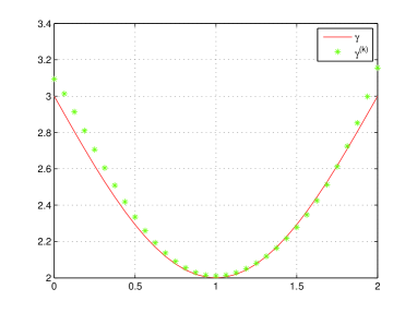
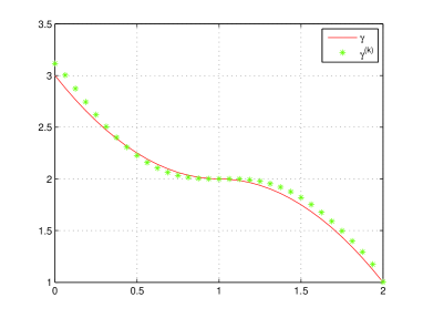
Figure 5.1: Exact and reconstructed Robin coefficients for Example 5.1 (left: $k=13$, the error $=0.0235$) and Example 5.2 (right: $k=19$, the error $=0.0270$).

Example 5.2.

We take the exact Robin coefficient $\gamma=(y-1)^{2}+2$ on $\{(x,y)\in\Gamma_{i};\,0\leq y\leq 1\}$ and $\gamma=-(y-1)^{2}+2$ on $\{(x,y)\in\Gamma_{i};\,1\leq y\leq 2\}$ and the initial guess $\gamma^{(0)}=2$.

Figure 5.1 (left) and Figure 5.1 (right) give respectively the exact and reconstructed Robin coefficients for Examples 5.1 and 5.2. We see from the figure that the numerical reconstructed Robin coefficients, with a $2\%$ noise in the data and very bad constant initial guesses, appear to be quite satisfactory, in view of the severe ill-posedness of the inverse Robin problem. We can also clearly see that Algorithms 3.1 converges quite fast with less than 20 iterations.

Next, we demonstrate two numerical examples of reconstructing the Robin coefficient $\gamma({\bf x})$ on the partial boundary $\Gamma_{i}=\{(x,y);~{}x=1,\,\,0\leq y\leq 2\}$ in the parabolic system (1.2) with $a({\bf x})=1$. We take the ambient temperature $g=(2+(\cos(\pi y)+1)\gamma({\bf x}))t$ on $\Gamma_{i}\times[0,T]$, the heat flux $h=0$ on $\Gamma_{a}\times[0,T]$, the source strength $f=\cos(\pi y)+x^{2}+(\pi^{2}\cos(\pi y)-2)t$ and the exact forward solution $u=(x^{2}+\cos(\pi y))t$ in $\Omega\times[0,T]$. We set the noise level $\delta=2\%$, the mesh $N=16$ and $M=32$, the tolerance parameter $\epsilon=5\times 10^{-3}$, the constant $A=1$ and the terminal time $T=2$.

Example 5.3.

We take the exact Robin coefficient $\gamma=-(y-1)^{2}+2$ and the initial guess $\gamma^{(0)}=2$.

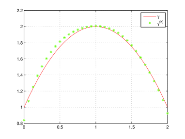
Figure 5.2: Exact and reconstructed Robin coefficients for Example 5.3 (left: $k=14$, the error $=0.0281$) and Example 5.4 (right: $k=12$, the error $=0.0270$)

Example 5.4.

We take the exact Robin coefficient $\gamma=\frac{1}{2}(\sin(\frac{\pi}{2}y)+y^{\frac{1}{4}})+1$ and the initial guess $\gamma^{(0)}=2$.

Figure 5.2 (left) and Figure 5.2 (right) give respectively the exact and reconstructed Robin coefficients for Examples 5.3 and 5.4. We see from the figure 5.2 that the numerical reconstructed Robin coefficients, with a $2\%$ noise in the data and very bad constant initial guesses, appear to be quite satisfactory, in view of the severe ill-posedness of the inverse Robin problem. And we also note that Algorithm 4.1 converges quite fast with less than 20 iterations.

6 Concluding remarks

We have justified in this work the uniqueness of the elliptic and parabolic Robin inverse problems. Then the Levenberg-Marquardt iterative method is formulated to solve the nonlinear Tikhonov regularized optimizations, which transform the original highly nonlinear and nonconvex minimizations into convex minimizations. We have established the quadratic convergence and the quadratic rate of convergence for the L-M iterations for the highly ill-posed nonlinear elliptic and parabolic Robin inverse problems. This appears to be the first time in literature to achieve the quadratic convergence and the quadratic rate of convergence for the L-M iterations rigorously for a highly nonlinear and ill-posed inverse problem, in combination with a simple and easily implementable choice rule of regularization parameters. The surrogate functional techniques have been applied to solve the convex minimizations at each L-M iteration, which lead to explicit expressions of the minimizers for both the elliptic and parabolic cases, resulting in two computationally very efficient solvers for the highly ill-posed nonlinear inverse problems. Numerical experiments have demonstrated the computational efficiency of the methods and their robustness against the noise in the observation data.

References

- [1] H.T. Banks and K. Kunisch, Estimation Techniques for Distributed Parameter Systems, Birkhauser, Boston, (1989).
- [2] S. Chaabane, J. Ferchichi and K. Kunisch, Differentiability properties of the -tracking functional and application to the Robin inverse problem, Inverse Problems, 20 (2004), 1083-1097.
- [3] I. Daubechies, M. Defrise, and C. DeMol, An iterative thresholding algorithm for linear inverse problems, Comm. Pure Appl. Math. 57 (2004), no. 11, 1413-1457.
- [4] J.Y. Fan and Y.X. Yuan, On the Quadratic Convergence of the Levenberg-Marquardt Method without Nonsingularity Assumption, Computing 74, 23-39 (2005).
- [5] W. Fang and M. Lu, A fast collocation method for an inverse boundary value problem, Int. J. Numer. Methods Eng., 59 (2004), 1563-1585.
- [6] M. Hanke, A regularization Levenberg-Marquardt scheme, with applications to inverse groundwater filtration problems, Inverse Problems 13 (1997), 79-95.
- [7] G. Inglese, An inverse problem in corrosion detection, Inverse Problems, 13 (1997), 977-994.
- [8] V. Isakov, Inverse Problems for Partial Differential Equations, 2nd edn. New York: Springer (2006).
- [9] D.J. Jiang and J. Zou, Local Lipschitz stability for inverse Robin problems in elliptic and parabolic systems, arXiv:1603.02556.
- [10] B. Jin, Conjugate gradient method for the Robin inverse problem associated with the Laplace equation, Int. J. Numer. Methods Eng., 71 (2007), 433-453.
- [11] B. Jin and X. Lu, Numerical identification of a Robin coefficient in parabolic problems, Math. Comput., 81 (2012), 1369-1398.
- [12] B. Jin and J. Zou, Numerical estimation of the Robin coefficient in a stationary diffusion equation, IMA J. Numer. Anal. 30 (2010), no. 3, 677-701.
- [13] K. Levenberg, A method for the solution of certain nonlinear problems in least squares, Quart. Appl. Math. 2 (1944), 164-166.
- [14] D.W. Marquardt, An algorithm for least-squares estimation of nonlinear inequalities, SIAM J. Appl. Math. 11 (1963), 431-441.
- [15] A.M. Osman and J.V. Beck, Nonlinear inverse problem for the estimation of time-and-space dependent heat transfer coefficients, J. Thermophys. Heat Transf., 3 (1989), 146-152.
- [16] N. Yamashita and M. Fukushima, On the rate of convergence of the Levenberg-Marquardt method, Computing (Suppl. 15): 237-249 (2001).