Millimeter Wave MIMO with Lens Antenna Array: A New Path Division Multiplexing Paradigm

Abstract

Millimeter wave (mmWave) communication over the largely unused mmWave spectrum is a promising technology for the fifth-generation (5G) cellular systems. To compensate for the severe path loss in mmWave communications, large antenna arrays are generally used at both the transmitter and receiver to achieve significant beamforming gains. However, the high hardware and power consumption cost due to the large number of radio frequency (RF) chains required renders the traditional beamforming method impractical for mmWave systems. It is thus practically valuable to achieve the large-antenna gains, but with only limited number of RF chains for mmWave communications. To this end, we study in this paper a new lens antenna array enabled mmWave multiple-input multiple-output (MIMO) communication system. We first show that the array response of the proposed lens antenna array at the receiver/transmitter follows a “sinc” function, where the antenna with the peak response is determined by the angle of arrival (AoA)/departure (AoD) of the received/transmitted signal. By exploiting this unique property of lens antenna arrays along with the multi-path sparsity of mmWave channels, we propose a novel low-cost and capacity-achieving MIMO transmission scheme, termed orthogonal path division multiplexing (OPDM). With OPDM, multiple data streams are simultaneously transmitted in parallel over different propagation paths with simple per-path signal processing at both the transmitter and receiver. For channels with insufficiently separated AoAs and/or AoDs, we also propose a simple path grouping technique with group-based small-scale MIMO processing to mitigate the inter-path interference. Numerical results are provided to compare the performance of the proposed lens antenna arrays for mmWave MIMO system against that of conventional arrays, under different practical setups. It is shown that the proposed system achieves significant throughput gain as well as complexity and hardware cost reduction, both making it an appealing new paradigm for mmWave MIMO communications.

I Introduction

The fifth-generation (5G) wireless communication systems on the roadmap are expected to provide at least 1000 times capacity increase over the current 4G systems [1]. To achieve this goal, various technologies have been proposed and extensively investigated during the past few years [2]. Among others, wireless communication over the largely unused millimeter wave (mmWave) spectrum (say, 30-300GHz) is regarded as a key enabling technology for 5G and has drawn significant interests recently (see [3, 4, 5, 6] and the references therein). Existing mmWave communication systems are designed mainly for short-range line-of-sight (LOS) indoor applications, e.g., wireless personal area networking (WPAN) [7] and wireless local area networking (WLAN) [8]. While recent measurement results have shown that, even in non-line-of-sight (NLOS) outdoor environment, mmWave signals with satisfactory strengths can be received up to 200 meters [9, 10], which indicates that mmWave communications may also be feasible for future cellular networks with relatively small cell coverage.

MmWave signals generally experience orders-of-magnitude more path loss than those at much lower frequency in existing cellular systems. On the other hand, their smaller wavelengths make it practically feasible to pack a large number of antennas with reasonable form factors at both the transmitter and receiver, whereby efficient MIMO (multiple-input multiple-output) beamforming techniques can be applied to achieve highly directional communication to compensate for the severe path loss [10, 11, 12, 13]. However, traditional MIMO beamforming is usually implemented digitally at baseband and thus requires one dedicated radio frequency (RF) chain for each transmit/receive antenna, which may not be feasible in mmWave systems due to the high hardware and power consumption cost of the large number of RF chains required. To reduce the cost and yet achieve the high array gain, analog beamforming has been proposed for mmWave communications [14, 15, 16], which can be implemented via phase shifters in the RF frontend, and thus requires only one RF chain for the entire transmitter/receiver. Despite of the notable cost reduction, analog beamforming usually incurs significant performance loss due to the constant-amplitude beamformer constraint imposed by the phase shifters, as well as its inability to perform spatial multiplexing for high-rate transmission. To enable spatial multiplexing, hybrid analog/digital precoding has been recently proposed [17, 18, 19, 20, 21, 22], where the precoding is implemented in two stages with a baseband digital precoding using a limited number of RF chains followed by a RF-band analog processing through a network of phase shifters. Since the hybrid precoding in general requires a large number of phase shifters, antenna subset selection has been proposed in [23] by replacing the phase shifters with switches. However, antenna selection may cause significant performance degradation due to the limited array gains resulted [24, 25], especially in highly correlated MIMO channels as in mmWave systems.

Besides, another promising line of research for mmWave or large MIMO systems aims to reduce signal processing complexity and RF chain cost without notable performance degradation by utilizing advanced antenna designs, such as the lens antenna array [26, 27, 28, 29, 30]. As shown in Fig. 1, a lens antenna array is in general composed of two main components: an electromagnetic (EM) lens and a matching antenna array with elements located in the focal region of the lens. Generally speaking, EM lenses can be implemented via three main technologies: i) the dielectric lenses made of dielectric materials with carefully designed front and/or rear surfaces [31, 32]; ii) the traditional planar lenses consisting of arrays of transmitting and receiving antennas connected via transmission lines with variable lengths [33, 34]; and iii) the modern planar lenses composed of sub-wavelength periodic inductive and capacitive structures [35, 36]. Regardless of the actual implementation methods, the fundamental principle of EM lenses is to provide variable phase shifting for EM rays at different points on the lens aperture so as to achieve angle of arrival (AoA)/departure (AoD)-dependent energy focusing, i.e., a receiving (transmitting) lens antenna array is able to focus (steer) the incident (departure) signals with sufficiently separated AoAs (AoDs) to (from) different antenna subsets. In [27], the concept of beamspace MIMO communication is introduced, where the lens antenna arrays are used to approximately transform the signals in antenna space to beamspace, which has much lower dimensions, to significantly reduce the number of RF chains required. However, the studies in [27] focus on the LOS mmWave channels, where spatial multiplexing is possible only for very short transmission range (e.g. a few meters) and/or extremely large antenna apertures. In a parallel work [29], the lens antenna array is applied to the massive MIMO cellular system with large number of antennas at the base station (BS) [37, 38, 39], which is shown to achieve significant performance gains as well as cost reduction as compared to the conventional arrays without lens. However, the result in [29] is only applicable for the single-input multiple-output (SIMO) uplink transmission, instead of the more general setup with lens antenna arrays applied at both the transmitter and receiver. Moreover, neither [27] nor [29] fully explores the characteristics of mmWave channels, such as the multi-path sparsity [5] due to limited scattering and the frequency selectivity in broadband transmission.

In this paper, we study the mmWave MIMO communication where both the transmitter and receiver are equipped with lens antenna arrays. Due to the AoA/AoD-dependent energy focusing, in mmWave systems with limited number of multi-paths, the signal power is generally focused on only a small subset of the antenna elements in the lens array; as a result, antenna selection can be applied to significantly reduce the RF chain cost, yet without notably comprising the system performance, which is in sharp contrast to the case of applying antenna selection with the conventional arrays [24, 25]. Furthermore, for mmWave channels with sufficiently separated AoAs/AoDs, different signal paths can be differentiated in the spatial domain with the use of the lens antenna array. Therefore, the detrimental multi-path effect in wide-band communications, i.e., the inter-symbol interference (ISI), can be easily alleviated in the lens array MIMO systems, without the need of sophisticated ISI mitigation techniques such as equalization, spread spectrum, or multi-carrier transmission [40]. In fact, in the favorable scenario where the AoAs/AoDs are sufficiently separated, the lens MIMO system can be shown to be equivalent to a set of parallel additive white Gaussian noise (AWGN) sub-channels, each corresponding to one of the multi-paths, for both narrow-band and wide-band communications. Thus, multiple data streams can be simultaneously multiplexed and transmitted over these sub-channels in parallel, each over one of the multi-paths with simple per-path processing. We term this new MIMO spatial multiplexing scheme enabled by the lens antenna array as orthogonal path division multiplexing (OPDM), in contrast to the conventional multiplexing techniques over orthogonal time or frequency. We summarize the main contributions of this paper as follows.

• First, we present the array configuration for the proposed lens antenna array in detail, and derive its corresponding array response. Our result shows that, different from the conventional arrays whose response is generally given by phase shifting across the antenna elements, the array response for the lens antennas follows a “sinc” function, where the antenna with peak response is determined by the AoA/AoD of the received/transmitted signal. This analytical result is consistent with that reported in prior works based on simulations [32, 30] or experiments [35]. With the derived array response, the channel model for the lens MIMO system is obtained, which is compared with that of a benchmark system using the conventional uniform planar arrays (UPAs).

• Next, to obtain fundamental limit and draw insight, we consider the so-called “ideal” AoA/AoD environment, where the signal power of each multi-path is focused on one single element of the lens array at the receiver/transmitter. We show that the channel capacity in this case is achieved by the novel OPDM scheme, which can be easily implemented by antenna selection with only $L$ transmitting/receiving RF chains, with $L$ denoting the number of multi-paths. Notice that $L$ is usually much smaller than the number of transmitting/receiving antennas in mmWave MIMO channels due to the multi-path sparsity. We further compare the lens array based mmWave MIMO system with that based on the conventional UPAs, in terms of capacity performance as well as signal processing complexity and RF chain cost.

• Finally, the mmWave lens MIMO is studied under the practical setup with multi-paths of arbitrary AoAs/AoDs. We propose a low-complexity transceiver design based on path-division multiplexing (PDM), applicable for both narrow-band and wide-band communications, with per-path maximal ratio transmission (MRT) at the transmitter and maximal ratio combining (MRC)/minimum mean square error (MMSE) beamforming at the receiver. We analytically show that in the case of wide-band communications, the proposed design achieves perfect ISI rejection if either the AoAs or AoDs (not necessarily both) of the multi-path signals are sufficiently separated, which usually holds in practice. Moreover, for cases with insufficiently separated AoAs and/or AoDs, we propose a simple path grouping technique with group-based small-scale MIMO processing to mitigate the inter-path interference.

It is worth pointing out that there has been an upsurge of interest recently in exploiting the angular domain of multi-path/multiuser signals in the design of massive MIMO systems. For example, by utilizing the fact that there is limited angular spread for signals sent from the mobile users, the authors in [41] propose a channel covariance-based pilot assignment strategy to mitigate the pilot contamination problem in multi-cell massive MIMO systems. Similarly in [42, 43], an AoA-based user grouping technique is proposed, which leads to the so-called joint spatial division and multiplexing scheme that makes massive MIMO also possible for frequency division duplexing (FDD) systems due to the significantly reduced channel estimation overhead after user grouping. In [44], an OFDM (orthogonal frequency division multiplexing) based beam division multiple access scheme is proposed for massive MIMO systems by simultaneously serving users with different beams at each frequency sub-channel. In this paper, we also exploit the different AoAs/AoDs of multi-path signals for complexity and cost reduction in mmWave MIMO systems, by utilizing the novel lens antenna arrays at both the transmitter and receiver.

The rest of this paper is organized as follows. Section II presents the array architecture as well as the array response function of the proposed lens antenna, based on which the MIMO channel model for mmWave communications is derived. The benchmark system using the conventional UPAs is also presented. In Section III, we consider the case of “ideal” AoA/AoD environment to introduce OPDM and demonstrate the great advantages of applying lens antenna arrays over conventional UPAs in mmWave communications. In Section IV, the practical scenario with arbitrary AoAs/AoDs is considered, where a simple transceiver design termed PDM applicable for both narrow-band and wide-band communications is presented, and a path grouping technique is proposed to further improve the performance. Finally, we conclude the paper and point out future research directions in Section V.

Notations: In this paper, scalars are denoted by italic letters. Boldface lower- and upper-case letters denote vectors and matrices, respectively. $\mathbb{C}^{M\times N}$ denotes the space of $M\times N$ complex-valued matrices, and $\mathbf{I}$ represents an identity matrix. For an arbitrary-size matrix $\mathbf{A}$, its complex conjugate, transpose, and Hermitian transpose are denoted by $\mathbf{A}^{*}$, $\mathbf{A}^{T}$, and $\mathbf{A}^{H}$, respectively. For a vector $\mathbf{a}$, $\|\mathbf{a}\|$ denotes its Euclidean norm, and $\mathrm{diag}{(\mathbf{a})}$ represents a diagonal matrix with the diagonal elements given in $\mathbf{a}$. For a non-singular square matrix $\mathbf{S}$, its matrix inverse is denoted as $\mathbf{S}^{-1}$. The symbol $j$ represents the imaginary unit of complex numbers, with $j^{2}=-1$. The notation $\circledast$ denotes the linear convolution operation. $\delta(\cdot)$ denotes the Dirac delta function, and $\mathrm{sinc}(\cdot)$ is the “sinc” function defined as $\mathrm{sinc}(x)\triangleq\sin(\pi x)/(\pi x)$. For a real number $a$, $\lfloor a\rfloor$ denotes the largest integer no greater than $a$, and $\mathrm{round}(a)$ represents the nearest integer of $a$. Furthermore, $U[a,b]$ represents the uniform distribution in the interval $[a,b]$. $\mathcal{N}(\boldsymbol{\mu},\mathbf{C})$ and $\mathcal{CN}(\boldsymbol{\mu},\mathbf{C})$ denote the real-valued Gaussian and the circularly symmetric complex-valued Gaussian (CSCG) distributions with mean $\boldsymbol{\mu}$ and covariance matrix $\mathbf{C}$, respectively. For a set $\mathcal{S}$, $|\mathcal{S}|$ denotes its cardinality. Furthermore, $\mathcal{S}_{1}\cap\mathcal{S}_{2}$ and $\mathcal{S}_{1}\cup\mathcal{S}_{2}$ denote the intersection and union of sets $S_{1}$ and $S_{2}$, respectively.

II System Description and Channel Model

II-A Lens Antenna Array

A lens antenna array in general consists of an EM lens and an antenna array with elements located in the focal region of the lens. Without loss of generality, we assume that a planar EM lens with negligible thickness and of size $D_{y}\times D_{z}$ is placed on the y-z plane and centered at the origin, as shown in Fig. 1. By considering only the azimuth AoAs and AoDs, the array elements are assumed to be placed on the focal arc of the lens, which is defined as a semi-circle around the lens’s center in the azimuth plane (i.e., x-y plane shown in Fig. 1) with radius $F$, where $F$ is known as the focal length of the lens. Therefore, the antenna locations relative to the lens center can be parameterized as $B_{m}(x_{m}=F\cos\theta_{m},y_{m}=-F\sin\theta_{m},z_{m}=0)$, where $\theta_{m}\in[-\pi/2,\pi/2]$ is the angle of the $m$th antenna element relative to the x-axis, $m\in\mathcal{M}$, with $\mathcal{M}\triangleq\{0,\pm 1,\cdots,\pm(M-1)/2\}$ denoting the set of antenna indices and $M$ representing the total number of antennas. Note that we have assumed that $M$ is an odd number for convenience. Furthermore, we assume the so-called critical antenna spacing, i.e., the antenna elements are deployed on the focal arc so that $\{\tilde{\theta}_{m}\triangleq\sin\theta_{m}\}$ are equally spaced in the interval $[-1,1]$ as

$$\tilde{\theta}_{m}=\frac{m}{\tilde{D}},\ m\in\mathcal{M},$$ (1)

where $\tilde{D}\triangleq D_{y}/\lambda$ is the effective lens dimension along the azimuth plane, with $\lambda$ denoting the carrier wavelength. It follows from (1) that $M$ and $\tilde{D}$ are related via $M=1+\lfloor 2\tilde{D}\rfloor$, i.e., more antennas should be deployed for larger lens dimension $\tilde{D}$. It is worth mentioning that with the array configuration specified in (1), antennas are more densely deployed in the center of the array than those on each of the two edges.

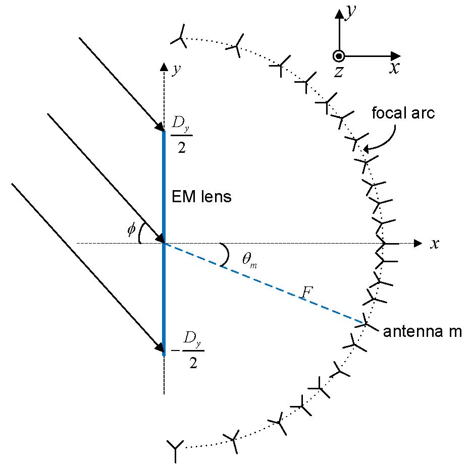
Figure 1: The schematic diagram of a lens antenna array with an incident uniform plane wave with AoA $\phi$.

We first study the receive array response by assuming that the lens antenna array is illuminated by a uniform plane wave with AoA $\phi$, as shown in Fig. 1. Denote by $x_{0}(\phi)$ the impinging signal at the reference point (say, the lens center) on the lens aperture, and $r_{m}(\phi)$ the resulting signal received by the $m$th element of the antenna array, $m\in\mathcal{M}$. The array response vector $\mathbf{a}(\phi)\in\mathbb{C}^{M\times 1}$, whose elements are defined by the ratio $a_{m}(\phi)\triangleq r_{m}(\phi)/x_{0}(\phi)$, can then be obtained in the following lemma.

Lemma 1

For the lens antenna array with critical antenna spacing as specified in (1), the receive array response vector $\mathbf{a}(\phi)$ as a function of the AoA $\phi$ is given by

$$a_{m}(\phi)=\sqrt{A}\mathrm{sinc}(m-\tilde{D}\tilde{\phi}),\ m\in\mathcal{M},$$ (2)

where $A\triangleq D_{y}D_{z}/\lambda^{2}$ is the effective aperture of the EM lens, and $\tilde{\phi}\triangleq\sin\phi\in[-1,1]$ is referred to as the spatial frequency corresponding to the AoA $\phi$.

Proof:

Please refer to Appendix A. ∎

Different from the traditional antenna arrays without lens, whose array responses are generally given by the simple phase shifting across different antenna elements (see e.g. (11) for the case of UPAs), the “$\mathrm{sinc}$”-function array response in (2) demonstrates the AoA-dependent energy-focusing capability of the lens antenna arrays, which is illustrated in Fig. 2. Specifically, for any incident signal with a given AoA $\phi$, the received power is magnified by approximately $A$ times for the receiving antenna located in the close vicinity of the focal point $\tilde{D}\tilde{\phi}$; whereas it is almost negligible for those antennas located far away from the focal point, i.e., antennas with $|m-\tilde{D}\tilde{\phi}|\gg 1$. As a result, any two simultaneously received signals with sufficiently different AoAs $\phi$ and $\phi^{\prime}$ such that $|\tilde{\phi}-\tilde{\phi}^{\prime}|\geq 1/\tilde{D}$ can be effectively separated in the spatial domain, as illustrated in Fig. 2 assuming a lens antenna array with $A=100$ and $\tilde{D}=10$ for two AoAs with $\sin\phi=0$ and $0.18$, respectively. Thus, we term the quantity $1/\tilde{D}$ as the array’s spatial frequency resolution, or approximately the AoA resolution for large $\tilde{D}$ [27].

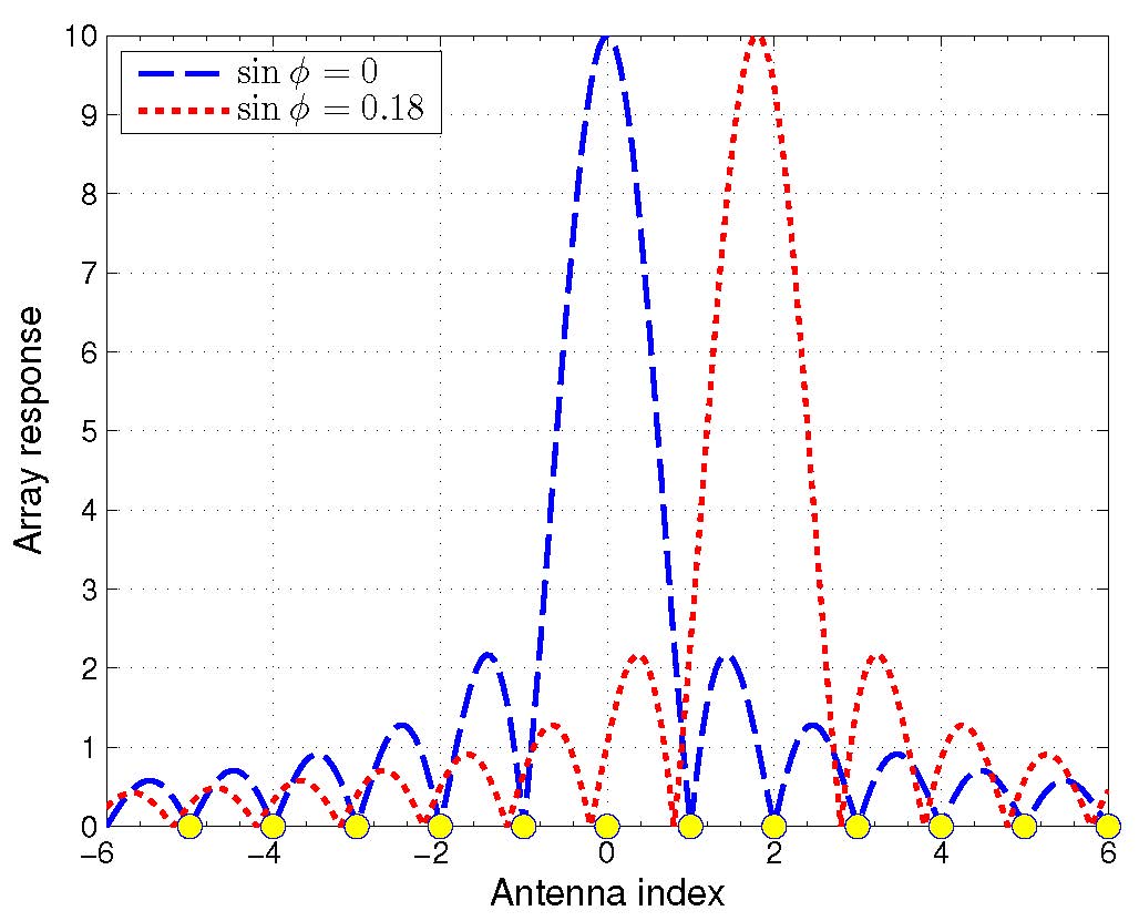
Figure 2: Array response of a lens antenna array with $A=100$ and $\tilde{D}=10$ for two different AoAs.

On the other hand, since the EM lens is a passive device, reciprocity holds between the incoming and outgoing signals through it. As a result, the transmit response vector for steering a signal towards the AoD $\phi$ can be similarly obtained by Lemma 1.

II-B Channel Model for MmWave Lens MIMO

In this subsection, we present the channel model for the mmWave lens MIMO system, where both the transmitter and receiver are equipped with lens antenna arrays with $Q$ and $M$ elements, respectively, as shown in Fig. 3. Under the general multi-path environment, the channel impulse response can be modeled as

$$\mathbf{H}(t) =\sum_{l=1}^{L}\alpha_{l}\mathbf{a}_{R}(\phi_{R,l})\mathbf{a}_{T}^{H}(\phi_{T,l})\delta(t-\tau_{l}),$$ (3)

where $\mathbf{H}(t)$ is an $M\times Q$ matrix with elements $h_{mq}(t)$ denoting the channel impulse response from transmitting antenna $q\in\mathcal{Q}$ to receiving antenna $m\in\mathcal{M}$, with $\mathcal{Q}$ and $\mathcal{M}$ respectively denoting the sets of the transmitting and receiving antenna indices as similarly defined in Section II-A; $L$ denotes the total number of significant multi-paths, which is usually small due to the multi-path sparsity in mmWave channels [5]; $\alpha_{l}$ and $\tau_{l}$ denote the complex-valued path gain and the delay for the $l$th path, respectively; $\phi_{R,l}$ and $\phi_{T,l}$ are the azimuth AoA and AoD for path $l$, respectively; and $\mathbf{a}_{R}\in\mathbb{C}^{M\times 1}$ and $\mathbf{a}_{T}\in\mathbb{C}^{Q\times 1}$ represent the array response vectors for the lens antenna arrays at the receiver and the transmitter, respectively. Note that in (3), we have assumed that the distances between the scatterers and the transmitter/receiver are much larger than the array dimensions, so that each multi-path signal can be well approximated as a uniform plane wave.

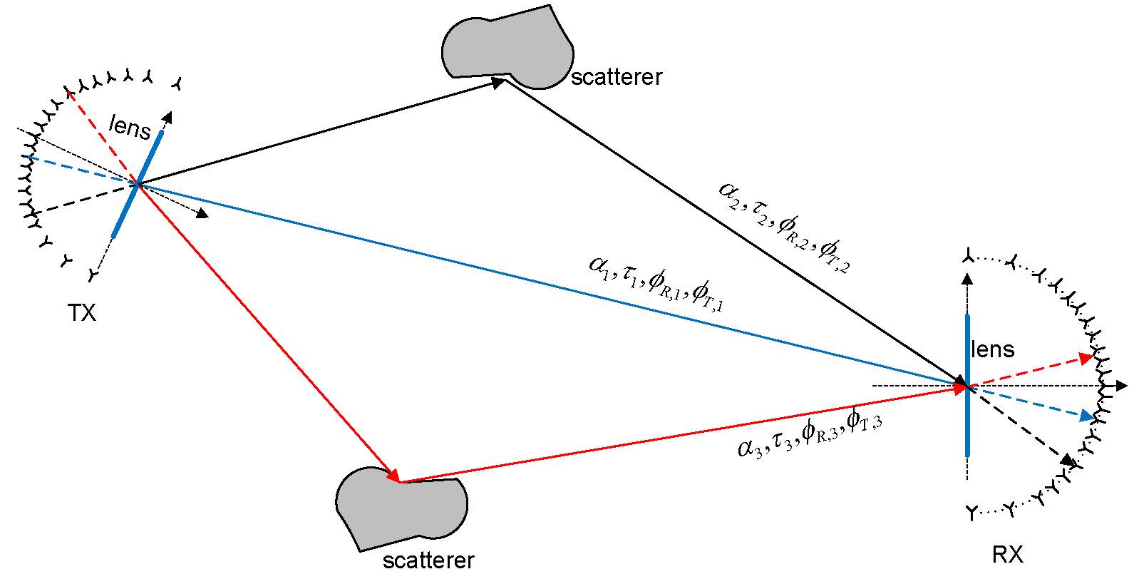
Figure 3: A mmWave lens MIMO system in multi-path environment.

Denote by $A_{T}$ and $A_{R}$ the effective lens apertures, and $\tilde{D}_{T}$ and $\tilde{D}_{R}$ the lens’s effective azimuth dimensions at the transmitter and at the receiver, respectively. Based on Lemma 1, the elements in the receive and transmit array response vectors $\mathbf{a}_{R}$ and $\mathbf{a}_{T}$ can be respectively expressed as

$$a_{R,m}(\phi_{R,l}) =\sqrt{A_{R}}\mathrm{sinc}(m-\tilde{D}_{R}\tilde{\phi}_{R,l}),\ m\in\mathcal{M},$$ (4)

$$a_{T,q}(\phi_{T,l}) =\sqrt{A_{T}}\mathrm{sinc}(q-\tilde{D}_{T}\tilde{\phi}_{T,l}),\ q\in\mathcal{Q},$$ (5)

where $\tilde{\phi}_{R,l}\triangleq\sin(\phi_{R,l})$ and $\tilde{\phi}_{T,l}\triangleq\sin(\phi_{T,l})$ are the AoA/AoD spatial frequencies of the $l$th path. Without loss of generality, $\tilde{\phi}_{R,l}$, $\tilde{\phi}_{T,l}\in[-1,1]$ of the $L$ multi-paths can be expressed in terms of the spatial frequency resolutions associated with the receiving/transmitting arrays as

$$\tilde{\phi}_{R,l}=\frac{m_{l}+\epsilon_{R,l}}{\tilde{D}_{R}},\ \tilde{\phi}_{T,l}=\frac{q_{l}+\epsilon_{T,l}}{\tilde{D}_{T}},\ l=1,\cdots,L,$$ (6)

where $m_{l}\in\mathcal{M}$ and $q_{l}\in\mathcal{Q}$ are integers given by $m_{l}=\mathrm{round}(\tilde{\phi}_{R,l}\tilde{D}_{R})$ and $q_{l}=\mathrm{round}(\tilde{\phi}_{T,l}\tilde{D}_{T})$; and $\epsilon_{R,l}$ and $\epsilon_{T,l}$ are fractional numbers in the interval $[-1/2,1/2]$. Intuitively, $m_{l}$ (or $q_{l}$) in (6) gives the receiving (transmitting) antenna index that is nearest to the focusing point corresponding to the AoA (AoD) of the $l$th path; whereas $\epsilon_{R,l}$ and $\epsilon_{T,l}$ represent the misalignment from the exact focusing point of the $l$th path signal relative to its nearest receiving/transmitting antenna. By substituting (6) into (4) and (5), the channel impulse response in (3) can be equivalently expressed as

$$h_{mq}(t) =\sum_{l=1}^{L}\alpha_{l}\sqrt{A_{R}A_{T}}\mathrm{sinc}(m-m_{l}-\epsilon_{R,l})$$ (7)

$$\times\mathrm{sinc}(q-q_{l}-\epsilon_{T,l})\delta(t-\tau_{l}),\ m\in\mathcal{M},q\in\mathcal{Q}.$$

Loosely speaking, (7) implies that the signal sent by the transmitting antenna with index $q=q_{l}$ will be directed towards the receiver mainly along the $l$th path, and be mainly focused on the receiving antenna with index $m=m_{l}$, as illustrated in Fig. 3.

With the channel impulse response matrix $\mathbf{H}(t)$ given in (3), the baseband equivalent signal received by the receiving lens antenna array can be expressed as

$$\mathbf{r}(t) =\mathbf{H}(t)\circledast\mathbf{x}(t)+\mathbf{z}(t)$$

$$=\sum_{l=1}^{L}\alpha_{l}\mathbf{a}_{R}(\phi_{R,l})\mathbf{a}_{T}^{H}(\phi_{T,l})\mathbf{x}(t-\tau_{l})+\mathbf{z}(t),$$ (8)

where $\mathbf{x}(t)\in\mathbb{C}^{Q\times 1}$ denotes the signal sent from the $Q$ transmitting antennas, and $\mathbf{z}(t)\in\mathbb{C}^{M\times 1}$ represents the AWGN vector at the receiving antenna array. In the special case of narrow-band communications where the maximum excessive delay of the multi-path signals is much smaller than the symbol duration $T_{s}$, i.e., $\underset{l\neq l^{\prime}}{\max}|\tau_{l}-\tau_{l^{\prime}}|\ll T_{s}\approx 1/W$ with $W$ denoting the signal bandwidth, we have $\tau_{l}\approx\tau$ and $\mathbf{x}(t-\tau_{l})\approx\mathbf{x}(t-\tau)$, $\forall l$. As a result, by assuming perfect time synchronization at the receiver, the general signal model for the wide-band communications in (8) reduces to

$$\mathbf{r}(t)=\mathbf{H}\mathbf{x}(t)+\mathbf{z}(t),$$ (9)

where $\mathbf{H}=\sum_{l=1}^{L}\alpha_{l}\mathbf{a}_{R}(\phi_{R,l})\mathbf{a}_{T}^{H}(\phi_{T,l})$ denotes the narrow-band MIMO channel.

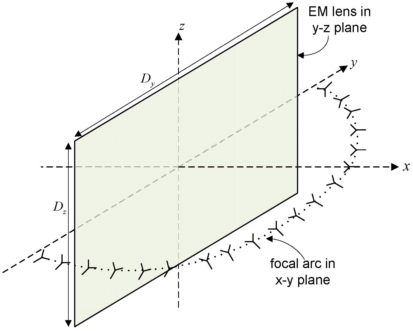
(a) Lens antenna array

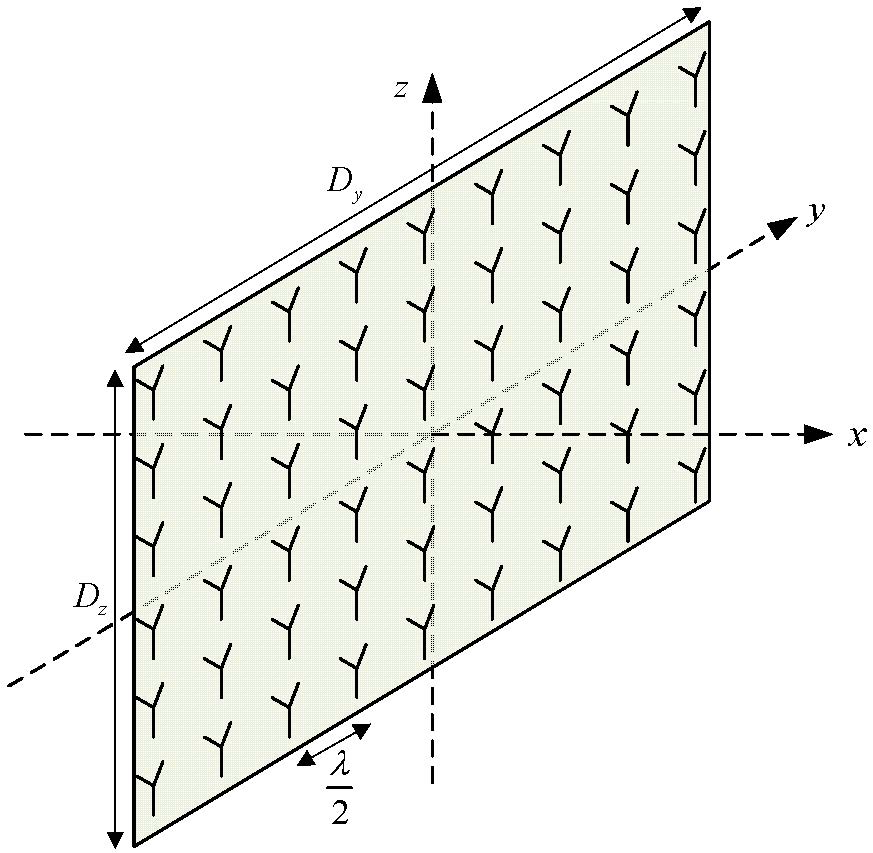
(b) Uniform planar array

Figure 4: 3D schematic diagrams of a lens antenna array versus an UPA with the same physical dimensions.

II-C Benchmark System: MmWave MIMO with Uniform Planar Array

As a benchmark system for comparison, we consider the mmWave communications in the traditional MIMO setup employing conventional antenna arrays without the EM lens. In particular, we assume that the transmitter and the receiver are both equipped with the UPAs with $Q_{\text{U}}$ and $M_{\text{U}}$ elements, respectively, with adjacent elements separated by distance $d_{\text{U}}=0.5\lambda$. For fair comparison, we assume that $Q_{\text{U}}$ and $M_{\text{U}}$ are designed such that the UPA has the same physical dimensions (or equivalently the same effective apertures $A_{T}$ and $A_{R}$) as the lens antenna of interest, as illustrated in Fig. 4. Accordingly, it can be obtained that $Q_{\text{U}}=D_{y}D_{z}/d_{\text{U}}^{2}=4A_{T}>Q$ and $M_{\text{U}}=4A_{R}>M$, i.e., in general more antennas need to be deployed in the conventional UPA than that in the lens antenna array to achieve the same array aperture, since the energy focusing capability of the EM lens effectively reduces the number of antenna elements required in lens array. This may compensate the additional cost of EM lens production and integration in practice. Denote by $\mathbf{H}_{\text{U}}(t)\in\mathbb{C}^{M_{\text{U}}\times Q_{\text{U}}}$ the channel impulse response matrix in the mmWave MIMO with UPAs. We then have

$$\mathbf{H}_{\text{U}}(t)=\sum_{l=1}^{L}\alpha_{l}\mathbf{a}_{R,\text{U}}(\phi_{R,l})\mathbf{a}_{T,\text{U}}^{H}(\phi_{T,l})\delta(t-\tau_{l}),$$ (10)

where $\alpha_{l},\tau_{l},\phi_{R,l}$ and $\phi_{T,l}$ are defined in (3), and $\mathbf{a}_{R,\text{U}}$ and $\mathbf{a}_{T,\text{U}}$ are the array response vectors corresponding to the UPAs at the receiver and transmitter, respectively, which are given by phase shifting across different antenna elements as [45]

$$\mathbf{a}_{R,\text{U}}(\phi) =\begin{matrix}\sqrt{\frac{A_{R}}{M_{\text{U}}}}\Big{[}1,&e^{j\Phi_{2}(\phi)},&\cdots&e^{j\Phi_{M_{\text{U}}}(\phi)}\Big{]}\end{matrix}^{T},$$ (11)

$$\mathbf{a}_{T,\text{U}}(\phi) =\begin{matrix}\sqrt{\frac{A_{T}}{Q_{\text{U}}}}\Big{[}1,&e^{j\Phi_{2}(\phi)},&\cdots&e^{j\Phi_{Q_{\text{U}}}(\phi)}\Big{]}\end{matrix}^{T},$$ (12)

with $\Phi_{m}$, $m=2,\cdots,M_{\text{U}}$ or $2,\cdots,Q_{\text{U}}$, denoting the phase shift of the $m$th array element relative to the first antenna. The input-output relationships for the UPA-based wide-band/narrow-band mmWave MIMO communications can be similarly obtained as in (8) and (9), respectively, and are thus omitted for brevity.

In this paper, we assume that the MIMO channel is perfectly known at the transmitter and receiver for both the proposed lens MIMO and the benchmark UPA-based MIMO systems.

III Lens MIMO under Ideal AoAs and AoDs

To demonstrate the fundamental gains of the lens MIMO based mmWave communication, we first consider an “ideal” multi-path propagation environment, where the spatial frequencies $\{\tilde{\phi}_{R,l},\tilde{\phi}_{T,l}\}_{l=1}^{L}$ corresponding to the AoAs/AoDs of the $L$ paths are all integer multiples of the spatial frequency resolutions of the receiving/transmitting lenses, i.e., $\{\epsilon_{R,l},\epsilon_{T,l}\}_{l=1}^{L}$ defined in (6) are all zeros. Furthermore, we assume that all the $L$ signal paths have distinct AoAs/AoDs such that $m_{l^{\prime}}\neq m_{l}$ and $q_{l^{\prime}}\neq q_{l}$, $\forall l^{\prime}\neq l$. In this case, we show that the multi-path signals in the lens antenna enabled mmWave MIMO system can be perfectly resolved in the spatial domain, thus leading to a new and capacity-achieving spatial multiplexing technique called OPDM. We also show that with OPDM, the lens antenna based mmWave MIMO system achieves the same (or even better) capacity performance in the narrow-band (wide-band) communications as compared to the conventional UPA based mmWave MIMO, but with dramatically reduced signal processing complexity and RF chain cost.

III-A Orthogonal Path Division Multiplexing

In the “ideal” AoA/AoD environment as defined above, the channel impulse response from the transmitting antenna $q$ to receiving antenna $m$ given in (7) reduces to

$$h_{mq}(t)=\sum_{l=1}^{L}\alpha_{l}\sqrt{A_{R}A_{T}}\delta(m-m_{l})\delta(q-q_{l})\delta(t-\tau_{l}).$$ (13)

The expression in (13) implies that the signal transmitted by antenna $q$ will be received at antenna $m$ if and only if there exists a propagation path such that the focusing points corresponding to its AoA and AoD align exactly with the locations of antenna $m$ and $q$, respectively, i.e., $m=m_{l}$ and $q=q_{l}$. Denote by $x_{q}(t)$ the signal sent by antenna $q$ of the transmitting lens array, where $q\in\mathcal{Q}$. The signal received by antenna $m$ (by ignoring additive noise for the time being) can then be expressed as

$$r_{m}(t) =\sum_{q\in\mathcal{Q}}h_{mq}(t)\circledast x_{q}(t)$$

$$=\begin{cases}\sqrt{A_{R}A_{T}}\alpha_{l}x_{q_{l}}(t-\tau_{l}),\ &\text{if }m=m_{l}\text{ for some }l,\\ 0,&\text{otherwise}.\end{cases}$$ (14)

Under the assumption of perfect time synchronization at each of the receiving antennas, i.e., $\tau_{l}$ is known at the receiver and perfectly compensated at antenna $m_{l}$, (14) can be equivalently written as

$$r_{m_{l}}=\sqrt{A_{R}A_{T}}\alpha_{l}x_{q_{l}}+z_{m_{l}},\ l=1,\cdots,L,$$ (15)

where $z_{m_{l}}$ denotes the AWGN at receiving antenna $m_{l}$. Therefore, the original multi-path MIMO channel has been decoupled into $L$ parallel SISO AWGN channels, each corresponding to one of the $L$ multi-paths. It is worth mentioning that the channel decomposition in (15) holds for both the narrow-band and wide-band communications. This thus enables a new low-complexity and cost-effective way to implement MIMO spatial multiplexing, by multiplexing $L$ data streams each over one of the $L$ multi-paths independently, which we term as OPDM.

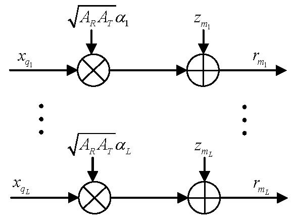
Figure 5: Equivalent input-output relationship for OPDM.

A schematic diagram of the equivalent input-output relationship for OPDM is shown in Fig. 5. It is straightforward to show that by applying the standard water-filling (WF) power allocation [40] over each of the $L$ parallel sub-channels with power gains $\{|\alpha_{l}|^{2}A_{R}A_{T}\}_{l=1}^{L}$, the capacity of the mmWave lens MIMO system can be achieved for both narrow-band and wide-band communications.

III-B Capacity Comparison

Next, we provide capacity comparison by simulations for the proposed lens MIMO versus the conventional UPA-based MIMO in mmWave communications. For the lens MIMO system, we assume that the transmitter and receiver lens apertures are both given by $A_{T}=A_{R}=20$, and the effective azimuth lens dimensions are $\tilde{D}_{T}=\tilde{D}_{R}=10$, which corresponds to the number of transmitting/receiving antennas as $M=Q=21$. For fair comparison, the UPA-based MIMO system is assumed to have the same array apertures as the lens MIMO, which thus needs $M_{\text{U}}=Q_{\text{U}}=80$ transmitting/receiving antennas, as discussed in Section II-C. We consider a mmWave channel of $L=3$ paths, which is typical in mmWave communications [5]. We assume a set of ideal AoAs/AoDs with $\tilde{\phi}_{T,l}=\tilde{\phi}_{R,l}\in\{0,\pm 0.2\}$. Furthermore, the complex-valued path gains $\{\alpha_{l}\}_{l=1}^{L}$ are modeled as $\alpha_{l}=\sqrt{\beta\kappa_{l}}e^{j\eta_{l}}$, $l=1,\cdots,L$ [9], where $\beta$ denotes the large-scale attenuation including distance-dependent path loss and shadowing, $\kappa_{l}$ represents the power fractional ratio for the $l$th path, with $\sum_{l=1}^{L}\kappa_{l}=1$, and $\eta_{l}\sim U[0,2\pi]$ denotes the phase shift of the $l$th path. The value of $\beta$ is set based on the generic model $-\beta_{\text{dB}}=c_{1}+10c_{2}\log_{10}(d)+\xi$, where $c_{1}$ and $c_{2}$ are the model parameters, $d$ is the communication distance in meters, and $\xi\sim\mathcal{N}(0,\epsilon^{2})$ denotes the lognormal shadowing. We assume that the system is operated at the mmWave frequency $f=73$ GHz, for which extensive channel measurements have been performed and the model parameters have been obtained as $c_{1}=86.6$, $c_{2}=2.45$, and $\epsilon=8$ dB [9]. Furthermore, we assume $d=100$ meters, with which the path loss is $136$ dB, or $\mathbb{E}[\beta]=-136$ dB, with the expectation taken over the log-normal shadowing. In addition, the multi-path power distribution $\{\kappa_{l}\}_{l=1}^{L}$ can be modeled as $\kappa_{l}=\frac{\kappa_{l}^{\prime}}{\sum_{k=1}^{L}\kappa_{k}^{\prime}}$, with $\kappa_{k}^{\prime}=U_{k}^{r_{\tau}-1}10^{-0.1Z_{k}}$, where $U_{k}\sim U[0,1]$ and $Z_{k}\sim\mathcal{N}(0,\zeta^{2})$ are random variables accounting for the variations in delay and in lognormal shadowing among different paths, respectively [9]. For mmWave channels at $f=73$ GHz, $r_{\tau}$ and $\zeta$ have been obtained as $r_{\tau}=3$ and $\zeta=4$ [9]. Furthermore, we assume that the total bandwidth is $W=500$ MHz, and the noise power spectrum density is $N_{0}=-174$ dBm/Hz. Denote by $P$ the total transmission power, the average signal-to-noise ratio (SNR) at each receiving array element (without the lens applied yet) is then defined as SNR$\triangleq P\mathbb{E}[\beta]/\sigma^{2}$. We consider two communication environments characterized by different values of the maximum multi-path excessive delays $T_{m}$, which correspond to: i) the narrow-band channel with $T_{m}\ll 1/W$; and ii) the wide-band channel with $T_{m}=100$ ns.

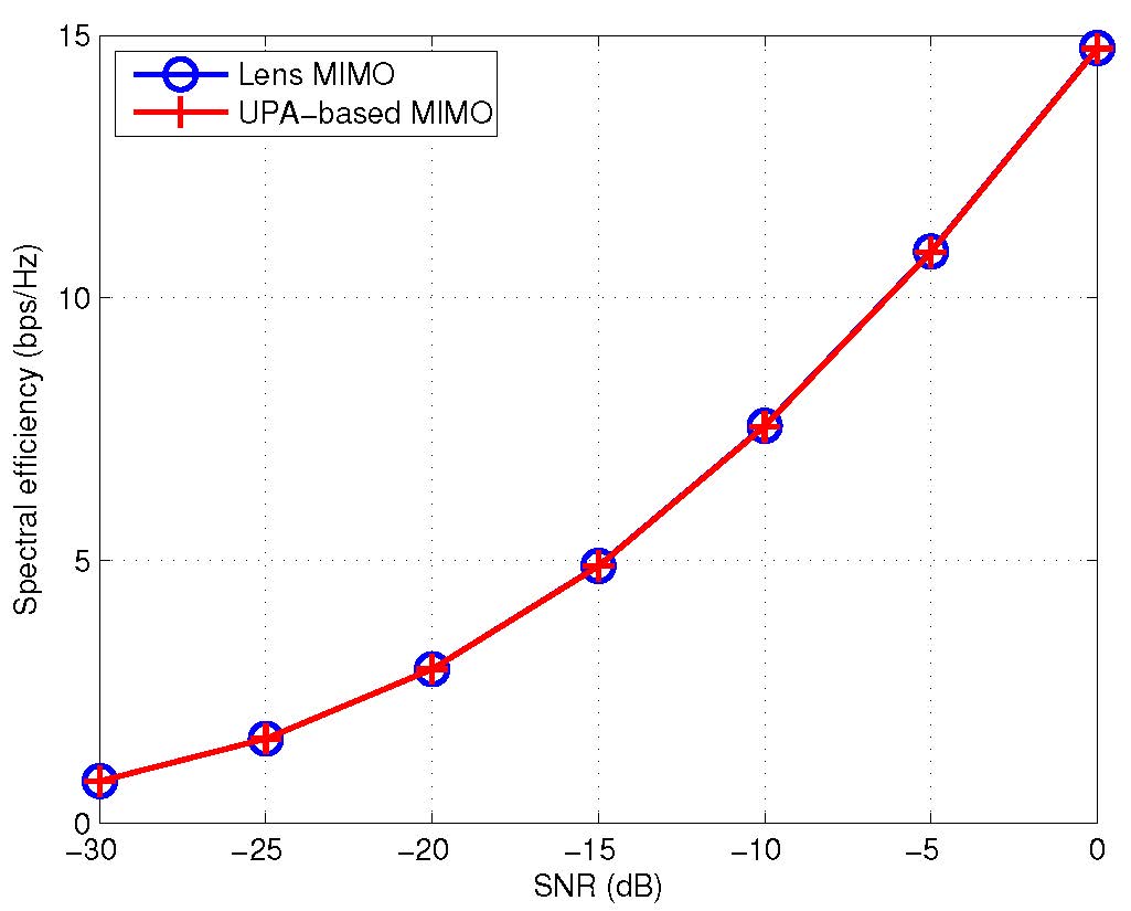
Figure 6: Capacity comparison of the lens MIMO using OPDM versus the UPA-based MIMO using eigenmode transmission in narrow-band mmWave communication.

In Fig. 6, the average spectrum efficiency is plotted against SNR for both the lens-based and the UPA-based mmWave MIMO systems in narrow-band communication, over $10^{4}$ random channel realizations. Note that for the UPA-based narrow-band MIMO system, the channel capacity is achieved by the well-known eigenmode transmission with WF power allocation based on singular value decomposition (SVD) over the MIMO channel matrix [40]. It is observed from Fig. 6 that under the ideal AoA/AoD environment, the lens MIMO using OPDM achieves almost the same capacity as that by the conventional UPA-based MIMO. However, their required signal processing complexity and hardware cost are rather different, as will be shown in the next subsection.

Fig. 7 compares the lens MIMO using OPDM versus the UPA-based MIMO using MIMO-OFDM in wide-band communication. For MIMO-OFDM, the total bandwidth is divided into $N=512$ orthogonal sub-bands, and a cyclic prefix (CP) of length $100$ ns is assumed. It is observed in Fig. 7 that for the wide-band communication case, the lens MIMO achieves higher capacity than the UPA-based MIMO, which is mainly due to the time overhead saved for CP transmission.

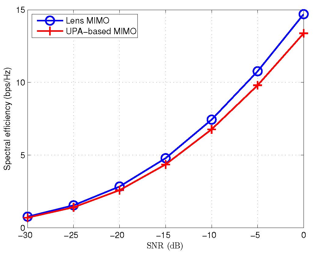
Figure 7: Capacity comparison of the lens MIMO using OPDM versus the UPA-based MIMO using MIMO-OFDM in wide-band mmWave communication.

TABLE I: Complexity and cost comparison for lens MIMO versus UPA-based MIMO.

	Signal Processing Complexity				Hardware Cost
	MIMO Processing		Channel Estimation		Antenna	RF chain
	Narrow-band	Wide-band	Narrow-band	Wide-band
Lens MIMO	$O(L)$	$O(L)$	$O(L)$	$O(L)$	$M+Q$	$2L$
UPA-based MIMO	$O(M_{\text{U}}Q_{\text{U}}L)$	$O(M_{\text{U}}Q_{\text{U}}LN+(Q_{\text{U}}+M_{\text{U}})N\log N)$	$O(M_{\text{U}}Q_{\text{U}})$	$O(M_{\text{U}}Q_{\text{U}}N)$	$M_{\text{U}}+Q_{\text{U}}$	$M_{\text{U}}+Q_{\text{U}}$

III-C Complexity and Cost Comparison

In this subsection, we compare the lens MIMO against the conventional UPA-based MIMO in mmWave communications in terms of signal processing complexity and hardware cost. The results are summarized in Table I and discussed in the following aspects:

• MIMO processing: For the lens MIMO based mmWave communication, the capacity for both the narrow-band and wide-band channels is achieved by the simple OPDM scheme, which can be efficiently implemented with signal processing complexity of $O(L)$, with $O(\cdot)$ representing the standard “big O” notation. In contrast, for the UPA-based mmWave MIMO communication, the capacity is achieved by the eigenmode transmission for narrow-band channel and approached by MIMO-OFDM for wide-band channel. The signal processing complexity for both schemes mainly arise from determining the eigen-space of the MIMO channel matrices, which has the complexity $O(M_{\text{U}}Q_{\text{U}}\min\{M_{\text{U}},Q_{\text{U}}\})$ for a generic matrix of size $M_{\text{U}}\times Q_{\text{U}}$ [46]. For a low-rank $M_{\text{U}}\times Q_{\text{U}}$ channel matrix of rank $L$, the complexity can be reduced to $O(M_{\text{U}}Q_{\text{U}}L)$ by exploiting its low-rank property [46]. Thus, the MIMO precoding/detection complexity for the UPA-based MIMO communication is $O(M_{\text{U}}Q_{\text{U}}L)$ and $O(M_{\text{U}}Q_{\text{U}}LN)$ in narrow-band and wide-band communications, respectively, where $N$ denotes the total number of sub-carriers in MIMO-OFDM, which in general requires additional complexity of $O((Q_{\text{U}}+M_{\text{U}})N\log N)$ at the transmitter and receiver for OFDM modulation/demodulation. As $L\ll\min\{M_{\text{U}},Q_{\text{U}}\}$ in mmWave communications, the lens MIMO has a significantly lower signal processing complexity than the UPA-based MIMO, especially for the wide-band communication case.

• Channel estimation: It follows from (15) that the lens MIMO using OPDM only requires estimating $L$ parallel SISO channels for both narrow-band and wide-band communications, which has a complexity $O(L)$. In contrast, the conventional UPA-based MIMO in general requires estimating the MIMO channel of size $M_{\text{U}}\times Q_{\text{U}}$ for narrow-band communication, and $N$ different MIMO channels each of size $M_{\text{U}}\times Q_{\text{U}}$ for wide-band communication using MIMO-OFDM.

• Hardware cost: The hardware cost for mmWave MIMO communications mainly depends on the required number of transmitting/receiving RF chains, which are composed of mixers, amplifiers, D/A or A/D converters, etc. For the lens MIMO system, it follows from (15) that only $L$ receiving/transmitting antennas located on the focusing points of the $L$ multi-paths need to be selected to operate at one time; whereas all the remaining antennas can be deactivated. This thus helps to significantly reduce the number of RF chains required as compared to the conventional UPA-based MIMO, as shown in Table I in detail.

IV Lens MIMO under Arbitrary AoAs/AoDs

In this section, we study the mmWave lens MIMO in the general channel with arbitrary AoAs/AoDs, i.e., the spatial frequencies $\{\tilde{\phi}_{R,l},\tilde{\phi}_{T,l}\}_{l=1}^{L}$ are not necessarily integer multiples of the spatial frequency resolutions of the receiving/transmitting lens arrays. In this case, the power for each multi-path signal in general spreads across the entire antenna array with decaying power levels from the antenna closest to the corresponding focusing point. Let $\Delta>0$ be a positive integer with which it can be practically approximated that $|\mathrm{sinc}(x)|^{2}\approx 0$, $\forall|x|\geq\Delta$. It then follows from (4) and (5) that the receive/transmit array responses for the $l$th path are negligible at those antennas with a distance greater than $\Delta$ from the focusing point (see Fig. 2), i.e.,

$$a_{R,m}(\phi_{R,l}) =\sqrt{A_{R}}\mathrm{sinc}(m-\tilde{D}_{R}\tilde{\phi}_{R,l})\approx 0,\quad\forall m\notin\mathcal{M}_{l},$$ (16)

$$a_{T,q}(\phi_{T,l}) =\sqrt{A_{T}}\mathrm{sinc}(q-\tilde{D}_{T}\tilde{\phi}_{T,l})\approx 0,\quad\forall q\notin\mathcal{Q}_{l},$$ (17)

where $\mathcal{M}_{l}$ and $\mathcal{Q}_{l}$ are referred to as the supporting receiving/transmitting antenna subsets for the $l$th path, which are defined as

$$\mathcal{M}_{l} \triangleq\left\{m\in\mathcal{M}:|m-\tilde{D}_{R}\tilde{\phi}_{R,l}|<\Delta\right\},$$ (18)

$$\mathcal{Q}_{l} \triangleq\left\{q\in\mathcal{Q}:|q-\tilde{D}_{T}\tilde{\phi}_{T,l}|<\Delta\right\},\ l=1,\cdots,L.$$ (19)

Consequently, the $(m,q)$-th element of the channel impulse response matrix $\mathbf{H}(t)$ in (3) has practically non-negligible power if and only if there exists at least one signal path $l$ such that $m\in\mathcal{M}_{l}$ and $q\in\mathcal{Q}_{l}$. Since $L\ll\min\{M,Q\}$ due to the multi-path sparsity in mmWave systems, it follows that $\mathbf{H}(t)$ is in practice a (nearly) sparse matrix with block sparsity structure, where each non-zero block corresponds to one of the $L$ multi-paths and has approximately $2\Delta\times 2\Delta$ entries around the element $(m_{l},q_{l})$, as illustrated in Fig. 8. Note that depending on the AoA/AoD values, $\{\mathcal{M}_{l}\}_{l=1}^{L}$ (or $\{\mathcal{Q}_{l}\}_{l=1}^{L}$) may have non-empty intersection for different paths, i.e., certain antenna elements may receive/transmit non-negligible power from/to more than one signal paths, as illustrated by $\mathcal{Q}_{2}$ and $\mathcal{Q}_{3}$ in Fig. 8.

Let $\mathcal{M}_{S}=\bigcup_{l=1}^{L}\mathcal{M}_{l}$ and $\mathcal{Q}_{S}=\bigcup_{l=1}^{L}\mathcal{Q}_{l}$ be the supporting receiving/transmitting antenna subsets associated with all the $L$ paths, and $\mathbf{H}_{S}(t)\in\mathbb{C}^{|\mathcal{M}_{S}|\times|\mathcal{Q}_{S}|}$ be the sub-matrix of the channel impulse response $\mathbf{H}(t)$ corresponding to the receiving antennas in $\mathcal{M}_{S}$ and transmitting antennas in $\mathcal{Q}_{S}$. By deactivating those antennas with negligible channel powers, the input-output relationship in (8) then reduces to

$$\mathbf{r}_{\mathcal{M}_{S}}(t) =\mathbf{H}_{S}(t)\circledast\mathbf{x}_{\mathcal{Q}_{S}}(t)+\mathbf{z}_{\mathcal{M}_{S}}(t)$$ (20)

$$=\sum_{l=1}^{L}\alpha_{l}\mathbf{a}_{R,\mathcal{M}_{S}}(\phi_{R,l})\mathbf{a}_{T,\mathcal{Q}_{S}}^{H}(\phi_{T,l})\mathbf{x}_{\mathcal{Q}_{S}}(t-\tau_{l})+\mathbf{z}_{\mathcal{M}_{S}}(t),$$ (21)

where $\mathbf{r}_{\mathcal{M}_{S}},\mathbf{a}_{R,\mathcal{M}_{S}},\mathbf{z}_{\mathcal{M}_{S}}\in\mathbb{C}^{|\mathcal{M}_{S}|\times 1}$ respectively denote the sub-vectors of $\mathbf{r},\mathbf{a}_{R}$ and $\mathbf{z}$ in (8) corresponding to the receiving antennas in $\mathcal{M}_{S}$; and $\mathbf{a}_{T,\mathcal{Q}_{S}},\mathbf{x}_{\mathcal{Q}_{S}}\in\mathbb{C}^{|\mathcal{Q}_{S}|\times 1}$ denote the sub-vectors of $\mathbf{a}_{T}$ and $\mathbf{x}$ corresponding to the transmitting antennas in $\mathcal{Q}_{S}$, respectively.

Remark 1

It follows from (21) that for mmWave lens MIMO system with arbitrary AoAs/AoDs, only $|\mathcal{M}_{S}|\ll M$ receiving and $|\mathcal{Q}_{S}|\ll Q$ transmitting RF chains are generally needed to achieve the near-optimal performance of the full-MIMO system with all $M+Q$ antennas/RF chains in use. Furthermore, since $|\mathcal{M}_{S}|\leq\sum_{l=1}^{L}|\mathcal{M}_{l}|\approx 2\Delta L$, and $|\mathcal{Q}_{S}|\leq\sum_{l=1}^{L}|\mathcal{Q}_{l}|\approx 2\Delta L$, the total number of RF chains required only depends on the number of multi-paths $L$, instead of the actually deployed antennas $M$ and $Q$.

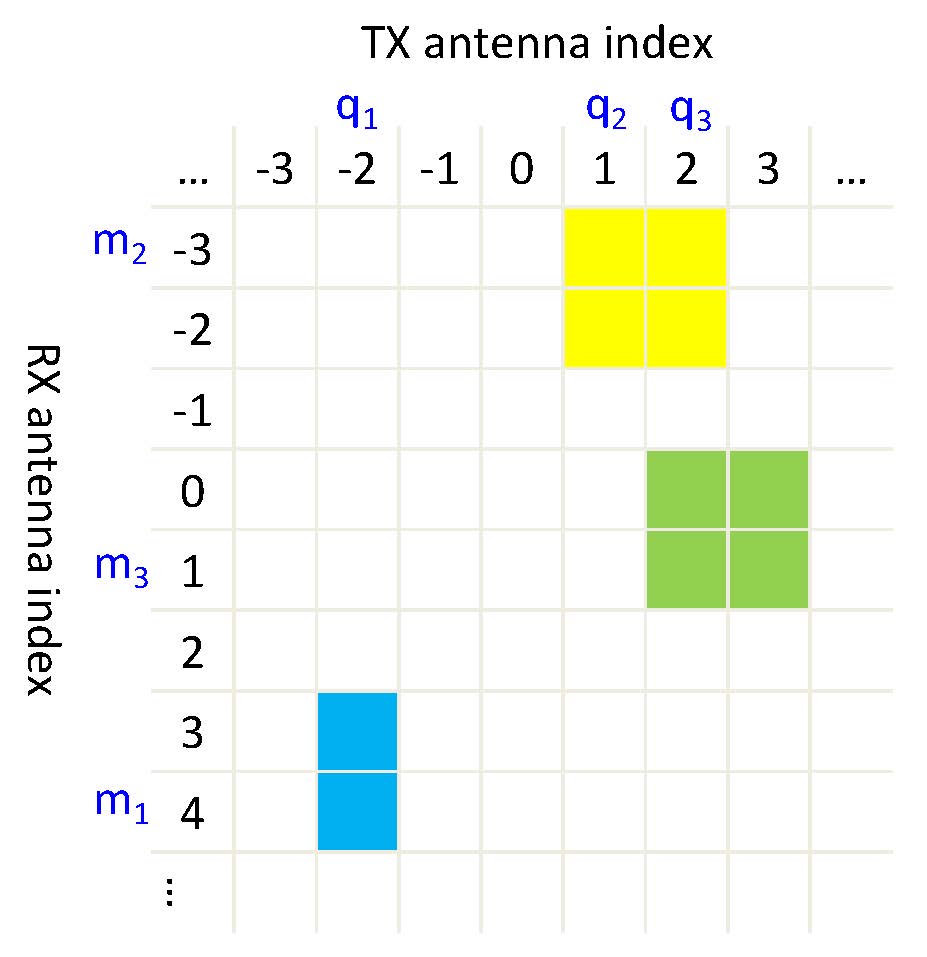
Figure 8: An illustration of the sparsity for a lens MIMO channel with $L=3$ paths. $\tilde{D}_{T}=\tilde{D}_{R}=10$. $\tilde{\phi}_{R,l}\in\{0.36,-0.27,0.08\}$, $\tilde{\phi}_{T,l}\in\{-0.2,0.12,0.24\}$. $\Delta=1$. $\mathcal{M}_{1}=\{3,4\},\mathcal{M}_{2}=\{-3,-2\},\mathcal{M}_{3}=\{0,1\},\mathcal{Q}_{1}=\{-2\},\mathcal{Q}_{2}=\{1,2\}$, and $\mathcal{Q}_{3}=\{2,3\}$. Note that $\mathcal{Q}_{2}\cap\mathcal{Q}_{3}\neq\emptyset$ due to the small AoD separation between path 2 and path 3.

IV-A Transceiver Design Based on PDM

In this subsection, by exploiting the reduced-size channel matrix in (21), we propose a low-complexity transceiver design based on PDM (instead of OPDM due to arbitrary AoAs/AoDs), which is applicable for both narrow-band and wide-band mmWave communications. With PDM, $L$ independent data streams are transmitted in general, each through one of the $L$ multi-paths by transmit beamforming/precoding. Specifically, the discrete-time equivalent of the transmitted signal $\mathbf{x}_{\mathcal{Q}_{S}}(t)$ can be expressed as

$$\mathbf{x}_{\mathcal{Q}_{S}}[n]=\sum_{l=1}^{L}\sqrt{\frac{p_{l}}{A_{T}}}\mathbf{a}_{T,\mathcal{Q}_{S}}(\phi_{T,l})s_{l}[n],$$ (22)

where $n$ denotes the symbol index, $s_{l}[n]\sim\mathcal{CN}(0,1)$ represents the i.i.d. CSCG distributed information-bearing symbols for data stream $l$, with transmit power $p_{l}$; and $\mathbf{a}_{T,\mathcal{Q}_{S}}(\phi_{T,l})/\sqrt{A_{T}}$ denotes the unit-norm per-path MRT beamforming vector towards the AoD $\phi_{T,l}$ of path $l$. Note that we have used the identity $\|\mathbf{a}_{T,\mathcal{Q}_{S}}(\phi_{T,l})\|^{2}\approx\|\mathbf{a}_{T}(\phi_{T,l})\|^{2}=A_{T}$, $\forall l$. At the receiver side, the low-complexity per-stream based detection is used, where a receiving beamforming vector $\mathbf{v}_{l}\in\mathbb{C}^{|\mathcal{M}_{S}|\times 1}$ with $\|\mathbf{v}_{l}\|=1$ is applied over the receiving antennas in $\mathcal{M}_{S}$ for detecting $s_{l}[n]$. Thus, we have

$$\hat{s}_{l}[n]=\mathbf{v}_{l}^{H}\mathbf{r}_{\mathcal{M}_{S}}[n],\ l=1,\cdots,L,$$ (23)

where $\mathbf{r}_{\mathcal{M}_{S}}[n]$ is the discrete-time equivalent of the received signal $\mathbf{r}_{\mathcal{M}_{S}}(t)$ shown in (21).

Next, we analyze the performance of the above proposed PDM scheme for wide-band communications. The analysis for the special case of narrow-band communications can be obtained similarly and is thus omitted for brevity. For simplicity, we assume that the multi-path delays can be approximated as integer multiples of the symbol interval $T_{s}$, i.e., $\tau_{l}=n_{l}T_{s}$ for some integer $n_{l}$, $\forall l$. For notational conciseness, let $\mathbf{a}_{T,l}\triangleq\mathbf{a}_{T,\mathcal{Q}_{S}}(\phi_{T,l})$ and $\mathbf{a}_{R,l}\triangleq\mathbf{a}_{R,\mathcal{M}_{S}}(\phi_{R,l})$, $\forall l$. Based on (21) and (22), the discrete-time equivalent received signal $\mathbf{r}_{\mathcal{M}_{S}}[n]$ can be expressed as

$$\mathbf{r}_{\mathcal{M}_{S}} [n]=\sum_{k=1}^{L}\alpha_{k}\mathbf{a}_{R,k}\mathbf{a}_{T,k}^{H}\mathbf{x}_{\mathcal{Q}_{S}}[n-n_{k}]+\mathbf{z}_{\mathcal{M}_{S}}[n]$$ (24)

$$= \underbrace{\sqrt{p_{l}A_{T}}\alpha_{l}\mathbf{a}_{R,l}s_{l}[n-n_{l}]}_{\text{desired signal}}+\underbrace{\sum_{k\neq l}^{L}\sqrt{\frac{p_{l}}{A_{T}}}\alpha_{k}\mathbf{a}_{R,k}\mathbf{a}_{T,k}^{H}\mathbf{a}_{T,l}s_{l}[n-n_{k}]}_{\text{ISI}}$$

$$+\underbrace{\sum_{l^{\prime}\neq l}^{L}\sum_{k=1}^{L}\sqrt{\frac{p_{l^{\prime}}}{A_{T}}}\alpha_{k}\mathbf{a}_{R,k}\mathbf{a}_{T,k}^{H}\mathbf{a}_{T,l^{\prime}}s_{l^{\prime}}[n-n_{k}]}_{\text{inter-stream interference}}+\mathbf{z}_{\mathcal{M}_{S}}[n].$$ (25)

Note that in (25), we have decomposed the received signal $\mathbf{r}_{\mathcal{M}_{S}}[n]$ from the perspective of the $l$th data stream, which includes the desired signal component propagated via the $l$th path with symbol delay $n_{l}$, the ISI from the same data stream received via all other $L-1$ paths with different delays, and the inter-stream interference from the other $L-1$ data streams. By applying the receiver beamforming in (23) and treating the ISI and the inter-stream interference both as noise, the effective SNR for the $l$th data stream can be expressed as (26) shown at the top of the next page.

$$\gamma_{l}=\frac{p_{l}A_{T}|\alpha_{l}|^{2}|\mathbf{v}_{l}^{H}\mathbf{a}_{R,l}|^{2}}{\sum_{k\neq l}^{L}\frac{p_{l}}{A_{T}}|\alpha_{k}|^{2}|\mathbf{v}_{l}^{H}\mathbf{a}_{R,k}|^{2}|\mathbf{a}_{T,k}^{H}\mathbf{a}_{T,l}|^{2}+\sum_{l^{\prime}\neq l}^{L}\sum_{k=1}^{L}\frac{p_{l^{\prime}}}{A_{T}}|\alpha_{k}|^{2}|\mathbf{v}_{l}^{H}\mathbf{a}_{R,k}|^{2}|\mathbf{a}_{T,k}^{H}\mathbf{a}_{T,l^{\prime}}|^{2}+\sigma^{2}},\forall l.$$ (26)

The achievable sum-rate is then given by $R=\sum_{l=1}^{L}\log_{2}(1+\gamma_{l})$. In the following, the two commonly used receiver beamforming schemes, i.e., MRC and MMSE beamforming, are studied to gain insights on the proposed PDM transmission scheme.

IV-A1 MRC Receive Beamforming

With MRC, the receiver beamforming vector $\mathbf{v}_{l}$ for data stream $l$ is set to maximize the desired signal power from the $l$th path, i.e., $\mathbf{v}_{l}^{\text{MRC}}=\mathbf{a}_{R,l}/\sqrt{A_{R}}$, $\forall l$. By substituting $\mathbf{v}_{l}^{\text{MRC}}$ into (26), the SNR can be expressed as (27) shown at the top of the next page.

$$\gamma_{l}^{\text{MRC}}=\frac{p_{l}|\alpha_{l}|^{2}A_{R}A_{T}}{\sum_{k\neq l}^{L}\frac{p_{l}}{A_{R}A_{T}}|\alpha_{k}|^{2}\left|\mathbf{a}_{R,l}^{H}\mathbf{a}_{R,k}\right|^{2}\left|\mathbf{a}_{T,k}^{H}\mathbf{a}_{T,l}\right|^{2}+\sum_{l^{\prime}\neq l}^{L}\sum_{k=1}^{L}\frac{p_{l^{\prime}}}{A_{R}A_{T}}|\alpha_{k}|^{2}\left|\mathbf{a}_{R,l}^{H}\mathbf{a}_{R,k}\right|^{2}\left|\mathbf{a}_{T,k}^{H}\mathbf{a}_{T,l^{\prime}}\right|^{2}+\sigma^{2}}.$$ (27)

 

Note that we have used the identity $\|\mathbf{a}_{R,l}\|^{2}\approx A_{R}$, $\forall l$. For two different paths $l^{\prime}\neq l$, define the transmitter and receiver side inter-path contamination (IPC) coefficients as

$$\rho_{T}^{ll^{\prime}}\triangleq\frac{\left|\mathbf{a}_{T,l}^{H}\mathbf{a}_{T,l^{\prime}}\right|^{2}}{A_{T}^{2}}<1,\quad\rho_{R}^{ll^{\prime}}\triangleq\frac{\left|\mathbf{a}_{R,l}^{H}\mathbf{a}_{R,l^{\prime}}\right|^{2}}{A_{R}^{2}}<1.$$ (28)

The SNR in (27) can then be simplified as

$$\gamma_{l}^{\text{MRC}} =\frac{p_{l}|\alpha_{l}|^{2}}{\sum_{k\neq l}^{L}p_{l}|\alpha_{k}|^{2}\rho_{R}^{lk}\rho_{T}^{kl}+\sum_{l^{\prime}\neq l}^{L}\sum_{k=1}^{L}p_{l^{\prime}}|\alpha_{k}|^{2}\rho_{R}^{lk}\rho_{T}^{kl^{\prime}}+\frac{\sigma^{2}}{A_{R}A_{T}}}$$ (29)

$$\approx\frac{p_{l}|\alpha_{l}|^{2}}{\sum_{k\neq l}^{L}p_{l}|\alpha_{k}|^{2}\rho_{R}^{lk}\rho_{T}^{kl}+\sum_{l^{\prime}\neq l}^{L}p_{l^{\prime}}\left(|\alpha_{l^{\prime}}|^{2}\rho_{R}^{ll^{\prime}}+|\alpha_{l}|^{2}\rho_{T}^{ll^{\prime}}\right)+\frac{\sigma^{2}}{A_{R}A_{T}}},$$ (30)

where the approximation in (30) is obtained by keeping only the two dominating inter-stream interference terms in (29) with either $k=l^{\prime}$ or $k=l$.

It is observed from (30) that for wide-band mmWave lens MIMO systems using PDM and the simple MRC receiver beamforming, the ISI is double attenuated as can be seen from the IPC coefficients $\rho_{T}^{kl}$ and $\rho_{R}^{lk}$ at both the transmitter and the receiver sides, and the inter-stream interference is attenuated through either transmitter-side IPC coefficient $\rho_{T}^{ll^{\prime}}$ or receiver-side IPC coefficient $\rho_{R}^{ll^{\prime}}$. Based on (5), we have

$$\rho_{T}^{ll^{\prime}} =\frac{1}{A_{T}^{2}}\left|\sum_{q\in\mathcal{Q}_{S}}a_{T,q}^{*}(\phi_{T,l})a_{T,q}(\phi_{T,l^{\prime}})\right|^{2}$$ (31)

$$=\left|\sum_{q\in\mathcal{Q}_{S}}\mathrm{sinc}(q-\tilde{D}_{T}\tilde{\phi}_{T,l})\mathrm{sinc}(q-\tilde{D}_{T}\tilde{\phi}_{T,l^{\prime}})\right|^{2},$$ (32)

which vanishes to zero for sufficiently separated AoDs such that $|\tilde{\phi}_{T,l}-\tilde{\phi}_{T,l^{\prime}}|>2\Delta/\tilde{D}_{T}$, or equivalently $\mathcal{Q}_{l}\cap\mathcal{Q}_{l^{\prime}}=\emptyset$. Similarly this holds for the receiver side IPC coefficient $\rho_{R}^{ll^{\prime}}$. In Fig. 9, the IPC coefficient $\rho_{T}^{ll^{\prime}}$ is plotted against the AoD difference $|\phi_{T,l}-\phi_{T,l^{\prime}}|$ for different AoD resolutions provided by the transmitter lens array, which verifies that the IPC vanishes asymptotically with large AoD separations and/or high AoD resolutions.

In the favorable propagation environment with both sufficiently separated AoAs and AoDs such that $\rho_{R}^{ll^{\prime}}\approx 0$ and $\rho_{T}^{ll^{\prime}}\approx 0$, $\forall l^{\prime}\neq l$, both the ISI and the inter-stream interference in (29) vanish. As a result, the SNR for the $l$th data stream reduces to $\gamma_{l}=p_{l}|\alpha_{l}|^{2}A_{R}A_{T}/\sigma^{2}$, $\forall l$, which is identical to that achieved by the OPDM in the ideal AoAs/AoDs case shown in Fig. 5. In this case, PDM with simple MRC receive beamforming achieves the channel capacity for both narrow-band and wide-band mmWave communications.

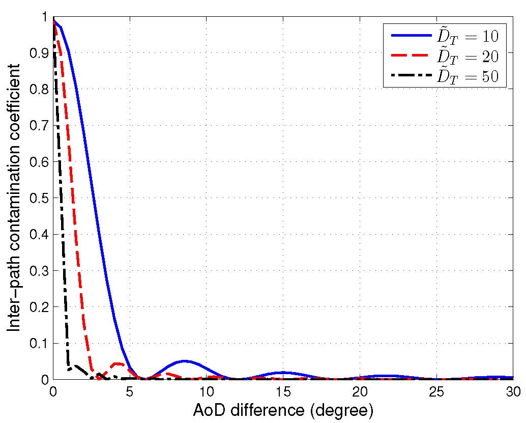
Figure 9: Transmitter-side inter-path contamination coefficient versus the AoD difference $|\phi_{T,l}-\phi_{T,l^{\prime}}|$ with different $\tilde{D}_{T}$ in lens MIMO systems.

IV-A2 MMSE Receive Beamforming

In the general case where the transmitter- and/or receiver-side IPC coefficients are non-zero due to the limited AoA/AoD separations and/or insufficient AoA/AoD resolutions provided by the lens arrays, the PDM scheme suffers from both ISI and inter-stream interference, which needs to be further mitigated. One simple interference mitigation scheme is via MMSE beamforming at the receiver, for which the beamforming vector $\mathbf{v}_{l}$ in (23) for the $l$th data stream is set as [47]

$$\mathbf{v}_{l}^{\text{MMSE}}=\frac{\mathbf{C}_{l}^{-1}\mathbf{a}_{R,l}}{\|\mathbf{C}_{l}^{-1}\mathbf{a}_{R,l}\|},\ l=1,\cdots,L,$$ (33)

where $\mathbf{C}_{l}$ is the covariance matrix of the effective noise vector. Based on (25), $\mathbf{C}_{l}$ can be obtained as (35) shown at the top of the next page,

$$\mathbf{C}_{l} =\sum_{k\neq l}^{L}\frac{p_{l}}{A_{T}}|\alpha_{k}|^{2}|\mathbf{a}_{T,k}^{H}\mathbf{a}_{T,l}|^{2}\mathbf{a}_{R,k}\mathbf{a}_{R,k}^{H}+\sum_{l^{\prime}\neq l}^{L}\sum_{k=1}^{L}\frac{p_{l^{\prime}}}{A_{T}}|\alpha_{k}|^{2}|\mathbf{a}_{T,k}^{H}\mathbf{a}_{T,l^{\prime}}|^{2}\mathbf{a}_{R,k}\mathbf{a}_{R,k}^{H}+\sigma^{2}\mathbf{I}$$ (34)

$$=\sum_{k\neq l}^{L}p_{l}A_{T}A_{R}|\alpha_{k}|^{2}\rho_{T}^{kl}\tilde{\mathbf{a}}_{R,k}\tilde{\mathbf{a}}_{R,k}^{H}+\sum_{l^{\prime}\neq l}^{L}\sum_{k=1}^{L}p_{l^{\prime}}A_{T}A_{R}|\alpha_{k}|^{2}\rho_{T}^{kl^{\prime}}\tilde{\mathbf{a}}_{R,k}\tilde{\mathbf{a}}_{R,k}^{H}+\sigma^{2}\mathbf{I},\forall l,$$ (35)

 

where $\tilde{\mathbf{a}}_{R,k}\triangleq\mathbf{a}_{R,k}/\sqrt{A_{R}}$, $k=1,\cdots,L$. The corresponding SNR can be obtained as

$$\gamma_{l}^{\text{MMSE}}= |\alpha_{l}|^{2}p_{l}A_{T}\mathbf{a}_{R,l}^{H}\mathbf{C}_{l}^{-1}\mathbf{a}_{R,l}$$ (36)

$$= |\alpha_{l}|^{2}p_{l}\tilde{\mathbf{a}}_{R,l}^{H}\Bigg{(}\sum_{k\neq l}^{L}p_{l}|\alpha_{k}|^{2}\rho_{T}^{kl}\tilde{\mathbf{a}}_{R,k}\tilde{\mathbf{a}}_{R,k}^{H}$$

$$+\sum_{l^{\prime}\neq l}^{L}\sum_{k=1}^{L}p_{l^{\prime}}|\alpha_{k}|^{2}\rho_{T}^{kl^{\prime}}\tilde{\mathbf{a}}_{R,k}\tilde{\mathbf{a}}_{R,k}^{H}+\frac{\sigma^{2}}{A_{T}A_{R}}\mathbf{I}\Bigg{)}^{-1}\tilde{\mathbf{a}}_{R,l}$$ (37)

$$\geq \gamma_{l}^{\text{MRC}},\ l=1,\cdots,L,$$ (38)

where (38) follows from the fact that $\mathbf{x}^{H}\mathbf{A}^{-1}\mathbf{x}\geq 1/(\mathbf{x}^{H}\mathbf{A}\mathbf{x})$, $\forall\|\mathbf{x}\|=1$. The inequality in (38) shows that MMSE beamforming in general achieves better performance than MRC, since it strikes a balance between maximizing the desired signal power and minimizing the interference. In the favorable scenario with both sufficiently separated AoAs and AoDs such that $\rho_{T}^{ll^{\prime}}\approx 0$ and $\rho_{R}^{ll^{\prime}}\approx 0$, $\forall l^{\prime}\neq l$, it can be shown that the MMSE and MRC receive beamforming vectors are identical.

IV-B Path Grouping

As can be seen from (29) and (37), the performance of the PDM scheme with MRC or MMSE receive beamforming depends on the ISI and inter-stream interference power via the IPC coefficients $\rho_{T}^{ll^{\prime}}$ and $\rho_{R}^{ll^{\prime}}$, $\forall l^{\prime}\neq l$. In this subsection, the PDM scheme is further improved by applying the technique of path grouping, by which the paths that are significantly interfered with each other are grouped and jointly processed. It is shown that the PDM with path-grouping achieves the channel capacity for both narrow-band and wide-band lens MIMO systems, provided that either the AoAs or AoDs (not necessarily both) are sufficiently separated.

IV-B1 Sufficiently Separated AoAs

We first consider the case with sufficiently separated AoAs for all paths such that $|\tilde{\phi}_{R,l}-\tilde{\phi}_{R,l^{\prime}}|>\frac{2\Delta}{\tilde{D}_{R}}$, $\forall l^{\prime}\neq l$, but with possibly close AoDs for certain paths. This may correspond to the uplink communications where the receiving lens antenna array equipped at the base station has a large azimuth dimension ($\tilde{D}_{R}\gg 1$) and hence provides accurate AoA resolution; whereas the transmitting lens array at the mobile terminal can only provide moderate AoD resolution. In this case, it follows from (18) that $\mathcal{M}_{l}\cap\mathcal{M}_{l^{\prime}}=\emptyset$, $\forall l^{\prime}\neq l$, i.e., $\left\{\mathcal{M}_{l}\right\}_{l=1}^{L}$ form a disjoint partition for the supporting receiving antenna subset $\mathcal{M}_{S}$. As a result, (21) can be decomposed into

$$\mathbf{r}_{\mathcal{M}_{l}}(t)=\alpha_{l}\mathbf{a}_{R,\mathcal{M}_{l}}(\phi_{R,l})\mathbf{a}_{T,\mathcal{Q}_{S}}^{H}(\phi_{T,l}) \mathbf{x}_{\mathcal{Q}_{S}}(t-\tau_{l})+\mathbf{z}_{\mathcal{M}_{l}}(t),$$

$$l=1,\cdots,L,$$ (39)

where $\mathbf{r}_{\mathcal{M}_{l}},\mathbf{a}_{R,\mathcal{M}_{l}},\mathbf{z}_{\mathcal{M}_{l}}\in\mathbb{C}^{|\mathcal{M}_{l}|\times 1}$ are respectively the sub-vectors of $\mathbf{r}_{\mathcal{M}_{S}},\mathbf{a}_{R,\mathcal{M}_{S}}$ and $\mathbf{z}_{\mathcal{M}_{S}}$ in (21) corresponding to the receiving antennas in $\mathcal{M}_{l}$. (39) shows that each receiving antenna only receives the signals via one of the multi-paths, thanks to the sufficient AoA separations such that the signals from different multi-paths are focused at non-overlapping receiving antenna subsets. However, the signal transmitted by certain transmitting antennas may propagate via more than one paths due to the possible overlapping of the supporting transmitting antenna subsets for different paths. Such a phenomenon is illustrated in Fig. 10.

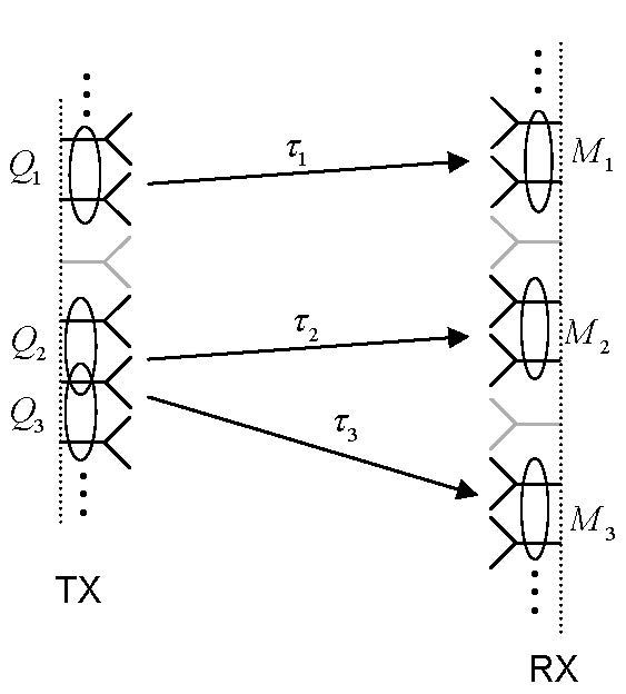
Figure 10: An illustration of the effective channel in mmWave lens MIMO system with sufficiently separated AoAs. The path delays are labeled for each link. Gray antennas represent those with negligible power and hence can be deactivated. Note that path $2$ and path $3$ are grouped since they have similar AoDs at Tx (but different AoAs at Rx).

Due to the single path received by each receiving antenna, the path delay $\tau_{l}$ can be compensated by the antennas in $\mathcal{M}_{l}$. As a result, (39) is equivalent to

$$\underbrace{\left[\begin{matrix}\mathbf{r}_{\mathcal{M}_{1}}\\ \vdots\\ \mathbf{r}_{\mathcal{M}_{L}}\end{matrix}\right]}_{\mathbf{r}_{\mathcal{M}_{S}}}=\underbrace{\left[\begin{matrix}\alpha_{1}\mathbf{a}_{R,\mathcal{M}_{1}}(\phi_{R,1})\mathbf{a}_{T,\mathcal{Q}_{S}}^{H}(\phi_{T,1})\\ \vdots\\ \alpha_{L}\mathbf{a}_{R,\mathcal{M}_{L}}(\phi_{R,L})\mathbf{a}_{T,\mathcal{Q}_{S}}^{H}(\phi_{T,L})\end{matrix}\right]}_{\mathbf{H}_{S}}\mathbf{x}_{\mathcal{Q}_{S}}+\underbrace{\left[\begin{matrix}\mathbf{z}_{\mathcal{M}_{1}}\\ \vdots\\ \mathbf{z}_{\mathcal{M}_{L}}\end{matrix}\right]}_{\mathbf{z}_{\mathcal{M}_{S}}}.$$ (40)

In other words, with sufficiently separated AoAs, the original multi-path channel in (21) is essentially equivalent to a simple MIMO AWGN channel given in (40), regardless of narrow-band or wide-band communications. The channel capacity of (40) is known to be achieved by the eigenmode transmission with WF power allocation based on the MIMO channel matrix $\mathbf{H}_{S}$. However, a closer look at $\mathbf{H}_{S}$ reveals that it is still a sparse matrix due to the sparsity of the transmitting response vectors $\mathbf{a}_{T,\mathcal{Q}_{S}}(\phi_{T,l})$, $\forall l$, which can be further exploited to reduce the complexity for achieving the capacity of the MIMO channel in (40).

Recall that the transmitting array response vector $\mathbf{a}_{T,\mathcal{Q}_{S}}(\phi_{T,l})$ has essentially non-zero entries only for those transmitting antennas in the subset $\mathcal{Q}_{l}\subseteq\mathcal{Q}_{S}$. The main idea for the proposed design is called AoD-based path grouping, by which the $L$ paths are partitioned into $G\leq L$ groups such that paths $l$ and $l^{\prime}$ belong to the same group if the transmitter-side IPC coefficient $\rho_{T}^{ll^{\prime}}>0$, or equivalently if $\mathcal{Q}_{l}\cap\mathcal{Q}_{l^{\prime}}\neq\emptyset$. Denote by $\mathcal{L}_{g}\subseteq\{1,\cdots,L\}$ the path indices in the $g$th group, $g=1,\cdots,G$. For instance, for the system shown in Fig. 10, we have $G=2$ and $\mathcal{L}_{1}=\{1\}$ and $\mathcal{L}_{2}=\{2,3\}$. In addition, denote by $\mathcal{\bar{Q}}_{g}\triangleq\bigcup_{l\in\mathcal{L}_{g}}\mathcal{Q}_{l}$ and $\bar{\mathcal{M}}_{g}\triangleq\bigcup_{l\in\mathcal{L}_{g}}\mathcal{M}_{l}$, $g=1,\cdots,G$, the supporting transmitting and receiving antenna subsets for all paths in group $g$, respectively. By construction, $\{\mathcal{\bar{Q}}_{g}\}_{g=1}^{G}$ and $\{\mathcal{\bar{M}}_{g}\}_{g=1}^{G}$ form disjoint partitions for the supporting transmitting antenna subsets $\mathcal{Q}_{S}$ and $\mathcal{M}_{S}$, respectively. Therefore, the input-output relationship in (40) can be decomposed into $G$ parallel MIMO AWGN channels as

$$\mathbf{r}_{\bar{\mathcal{M}}_{g}}=\bar{\mathbf{H}}_{g}\mathbf{x}_{\bar{\mathcal{Q}}_{g}}+\mathbf{z}_{\bar{\mathcal{M}}_{g}},\ g=1,\cdots,G,$$ (41)

where $\mathbf{r}_{\bar{\mathcal{M}}_{g}},\mathbf{z}_{\bar{\mathcal{M}}_{g}}\in\mathbb{C}^{|\bar{\mathcal{M}}_{g}|\times 1}$ and $\mathbf{x}_{\bar{\mathcal{Q}}_{g}}\in\mathbb{C}^{|\bar{\mathcal{Q}}_{g}|\times 1}$ denote the sub-vectors of $\mathbf{r}_{\mathcal{M}_{S}}$, $\mathbf{z}_{\mathcal{M}_{S}}$ and $\mathbf{x}_{\mathcal{Q}_{S}}$ in (40), respectively; and $\bar{\mathbf{H}}_{g}\triangleq\sum_{l\in\mathcal{L}_{g}}\alpha_{l}\mathbf{a}_{R,\bar{\mathcal{M}}_{g}}(\phi_{R,l})\mathbf{a}_{T,\bar{\mathcal{Q}}_{g}}^{H}(\phi_{T,l})$ denotes the corresponding MIMO channel matrix for group $g$. The channel capacity of (41) is then achieved by the eigenmode transmission over each of the $G$ parallel MIMO channels, which have smaller dimension and hence require lower complexity as compared to the original channel in (40) without path grouping.

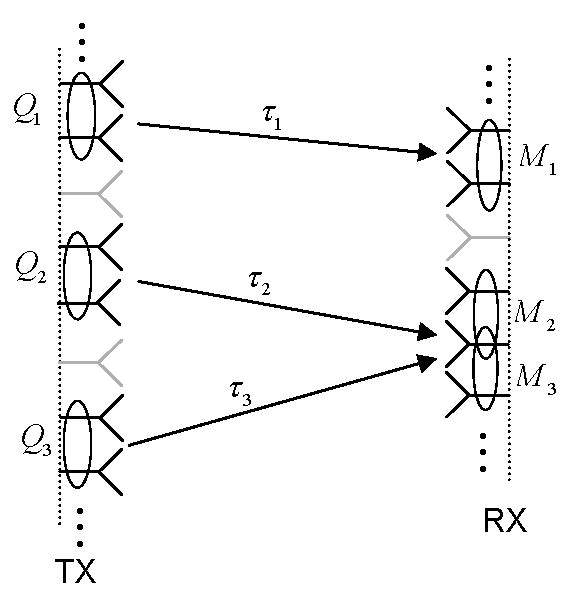
Figure 11: An illustration of the effective channel in mmWave lens MIMO system with sufficiently separated AoDs. The path delays are labeled for each link. Gray antennas represent those with negligible power and hence can be deactivated. Note that path $2$ and path $3$ are grouped since they have similar AoAs at Rx (but different AoDs at Tx).

IV-B2 Sufficiently Separated AoDs

Next, we consider the case with sufficiently separated AoDs for all paths such that $|\tilde{\phi}_{T,l}-\tilde{\phi}_{T,l^{\prime}}|>2\Delta/\tilde{D}_{T}$, or $\mathcal{Q}_{l}\cap\mathcal{Q}_{l^{\prime}}=\emptyset$, $\forall l\neq l^{\prime}$, but with possibly close AoAs for certain paths. This may correspond to the downlink transmission with accurate AoD resolution ($\tilde{D}_{T}\gg 1$) at the base station transmitter, but with only moderate AoA resolution at the mobile terminal receiver. In this case, $\{\mathcal{Q}_{l}\}_{l=1}^{L}$ form a disjoint partition for the transmitting antenna subset $\mathcal{Q}_{S}$, and the input-output relationship in (21) can be re-written as

$$\mathbf{r}_{\mathcal{M}_{S}}(t)=\sum_{l=1}^{L}\alpha_{l}\mathbf{a}_{R,\mathcal{M}_{S}}(\phi_{R,l})\mathbf{a}_{T,\mathcal{Q}_{l}}^{H}(\phi_{T,l})\mathbf{x}_{\mathcal{Q}_{l}}(t-\tau_{l})+\mathbf{z}_{\mathcal{M}_{S}}(t).$$ (42)

The expression in (42) shows that the signals sent by each transmitting antenna arrive at the receiver only via one of the multi-paths, as illustrated in Fig. 11. This thus provides the opportunity for path delay pre-compensation at the transmitter by setting the transmitted signal as $\mathbf{x}_{\mathcal{Q}_{l}}(t)=\mathbf{x}_{\mathcal{Q}_{l}}^{\prime}(t+\tau_{l})$, $\forall l$. As a result, (42) can be equivalently written as (43) shown at the top of the next page.

$$\mathbf{r}_{\mathcal{M}_{S}}=\underbrace{\left[\begin{matrix}\alpha_{1}\mathbf{a}_{R,\mathcal{M}_{S}}(\phi_{R,1})\mathbf{a}_{T,\mathcal{Q}_{1}}^{H}(\phi_{T,1})&\cdots&\alpha_{L}\mathbf{a}_{R,\mathcal{M}_{S}}(\phi_{R,L})\mathbf{a}_{T,\mathcal{Q}_{L}}^{H}(\phi_{T,L})\end{matrix}\right]}_{\mathbf{H}_{S}}\underbrace{\left[\begin{matrix}\mathbf{x}_{\mathcal{Q}_{1}}^{\prime}\\ \vdots\\ \mathbf{x}_{\mathcal{Q}_{L}}^{\prime}\end{matrix}\right]}_{\mathbf{x}_{\mathcal{Q}_{S}}^{\prime}}+\mathbf{z}_{\mathcal{M}_{S}}.$$ (43)

 

Similar to the previous subsection, (43) shows that with sufficiently separated AoDs, the lens MIMO system is equivalent to a $|\mathcal{M}_{S}|\times|\mathcal{Q}_{S}|$ MIMO AWGN channel. This holds regardless of narrow-band or wide-band communications. The channel capacity of (43) is achievable by eigenmode transmission with WF power allocation based on the equivalent channel matrix $\mathbf{H}_{S}$. Similar to Section IV-B1, by exploiting the channel sparsity of $\mathbf{H}_{S}$, we can design a low-complexity capacity-achieving scheme by employing the AoA-based path-grouping at the receiver side. Specifically, the $L$ signal paths are partitioned into $G\leq L$ groups such that paths $l$ and $l^{\prime}$ belong to the same group if their supporting receiving antenna subsets have non-empty overlapping, i.e., $\mathcal{M}_{l}\cap\mathcal{M}_{l^{\prime}}\neq\emptyset$. Denote by $\mathcal{L}_{g}\subseteq\{1,\cdots,L\}$, $g=1,\cdots,G$, the subset containing all paths in group $g$. For instance, for the system shown in Fig. 11, we have $G=2$ and $\mathcal{L}_{1}=\{1\}$ and $\mathcal{L}_{2}=\{2,3\}$. In addition, denote by $\mathcal{\bar{Q}}_{g}\triangleq\bigcup_{l\in\mathcal{L}_{g}}\mathcal{Q}_{l}$ and $\bar{\mathcal{M}}_{g}\triangleq\bigcup_{l\in\mathcal{L}_{g}}\mathcal{M}_{l}$, $g=1,\cdots,G$, the supporting transmitting and receiving antenna subsets for all paths in group $g$, respectively. Similar to Section IV-B1, the input-output relationship in (43) can then be decomposed into $G$ parallel MIMO AWGN channels as

$$\mathbf{r}_{\bar{\mathcal{M}}_{g}}=\bar{\mathbf{H}}_{g}\mathbf{x}_{\bar{\mathcal{Q}}_{g}}^{\prime}+\mathbf{z}_{\bar{\mathcal{M}}_{g}},\ g=1,\cdots,G,$$ (44)

where $\mathbf{r}_{\bar{\mathcal{M}}_{g}},\mathbf{z}_{\bar{\mathcal{M}}_{g}}\in\mathbb{C}^{|\bar{\mathcal{M}}_{g}|\times 1}$ and $\mathbf{x}_{\bar{\mathcal{Q}}_{g}}^{\prime}\in\mathbb{C}^{|\bar{\mathcal{Q}}_{g}|\times 1}$ denote the sub-vectors of $\mathbf{r}_{\mathcal{M}_{S}}$, $\mathbf{z}_{\mathcal{M}_{S}}$ and $\mathbf{x}_{\mathcal{Q}_{S}}^{\prime}$ in (43), respectively; and $\bar{\mathbf{H}}_{g}\triangleq\sum_{l\in\mathcal{L}_{g}}\alpha_{l}\mathbf{a}_{R,\bar{\mathcal{M}}_{g}}(\phi_{R,l})\mathbf{a}_{T,\bar{\mathcal{Q}}_{g}}^{H}(\phi_{T,l})$ denotes the corresponding MIMO channel matrix for group $g$. The channel capacity of (44) is then achieved by the eigenmode transmission over each of the $G$ parallel MIMO channels each with reduced size.

IV-C Numerical Results

In this subsection, we evaluate the performance of the proposed PDM in a wide-band mmWave lens MIMO system by numerical examples. We assume that the lens apertures at the transmitter and receiver are $A_{T}=100$ and $A_{R}=50$, respectively, and the azimuth lens dimensions are $\tilde{D}_{T}=20$ and $\tilde{D}_{R}=10$, respectively. Accordingly, the number of transmitting and receiving antennas in the lens MIMO systems are $Q=41$ and $M=21$, respectively. For the benchmark MIMO system based on the conventional UPAs, the number of transmitting and receiving antennas are set as $Q_{\text{U}}=400$ and $M_{\text{U}}=200$, respectively, for achieving the same antenna apertures as the lens MIMO system. For both the lens MIMO and UPA-based MIMO systems, antenna selections are applied by assuming that the number of RF chains at the transmitter and receiver are $M_{\text{RF}}=Q_{\text{RF}}=2\Delta L$, where $L$ is the number of multi-paths and $\Delta$ is a design parameter to achieve a reasonable balance between performance and RF chain cost. We set $\Delta=1$ in this example. For the lens MIMO system, the AoA/AoD based antenna selection method given in (18) and (19) are applied at the receiver and transmitter, respectively. However, since the optimal antenna scheme for the UPA-based MIMO-OFDM system is unknown in general, we adopt the power-based antenna selection due to its simplicity and good performance [25]. We assume that the mmWave channel has $L=3$ paths with AoDs given by $\phi_{T,l}\in\{-15^{\circ},10^{\circ},45^{\circ}\}$, which are sufficiently separated based on the criterion specified in Section IV-B2. On the other hand, the AoAs of the $L$ paths are assumed to be equally spaced in the interval $[-\Phi_{R}/2,\Phi_{R}/2]$, with $\Phi_{R}$ referred to as the AoA angular spread. Furthermore, the maximum multi-path delay is assumed to be $T_{m}=100$ ns and the total available bandwidth is $W=500$ MHz, which is divided into $N=512$ sub-carriers for the UPA-based MIMO-OFDM. The CP length for the OFDM is set as $100$ ns.

In Fig. 12, the spectrum efficiency achieved by different schemes is shown for the mmWave communication with AoA angular spread $\Phi_{R}=150^{\circ}$. Note that for simplicity the power allocation $\{p_{l}\}_{l=1}^{L}$ for the PDM with MRC and MMSE receive beamforming is obtained via WF by assuming $L$ parallel SISO channels with power gains $\{|\alpha_{l}|^{2}A_{R}A_{T}\}_{l=1}^{L}$. It is observed from Fig. 12 that the UPA-based MIMO-OFDM gives rather poor performance, which is expected due to the limited array gain with the small number of antennas selected. In contrast, the lens MIMO systems with the three proposed PDM schemes achieve significant rate improvement over the UPA-based MIMO-OFDM with the same number of RF chains used or antennas selected. Moreover, Fig. 12 shows that in the low-SNR regime, PDM with the simple MMSE and MRC receive beamforming achieves the same performance as that with path grouping, which is expected due to the negligible inter-path interference in the low-SNR regime. While as the SNR increases, the three PDM schemes show more different performances due to their different interference mitigation capabilities. The performance gaps are more pronounced for systems with smaller AoA separations, as shown in Fig. 13 for $\Phi_{R}=10^{\circ}$ as compared to Fig. 12 for $\Phi_{R}=150^{\circ}$. This implies the necessity of more sophisticated interference mitigation techniques (such as path grouping) for PDM when the paths are severely coupled with each other due to the limited AoA/AoD separations.

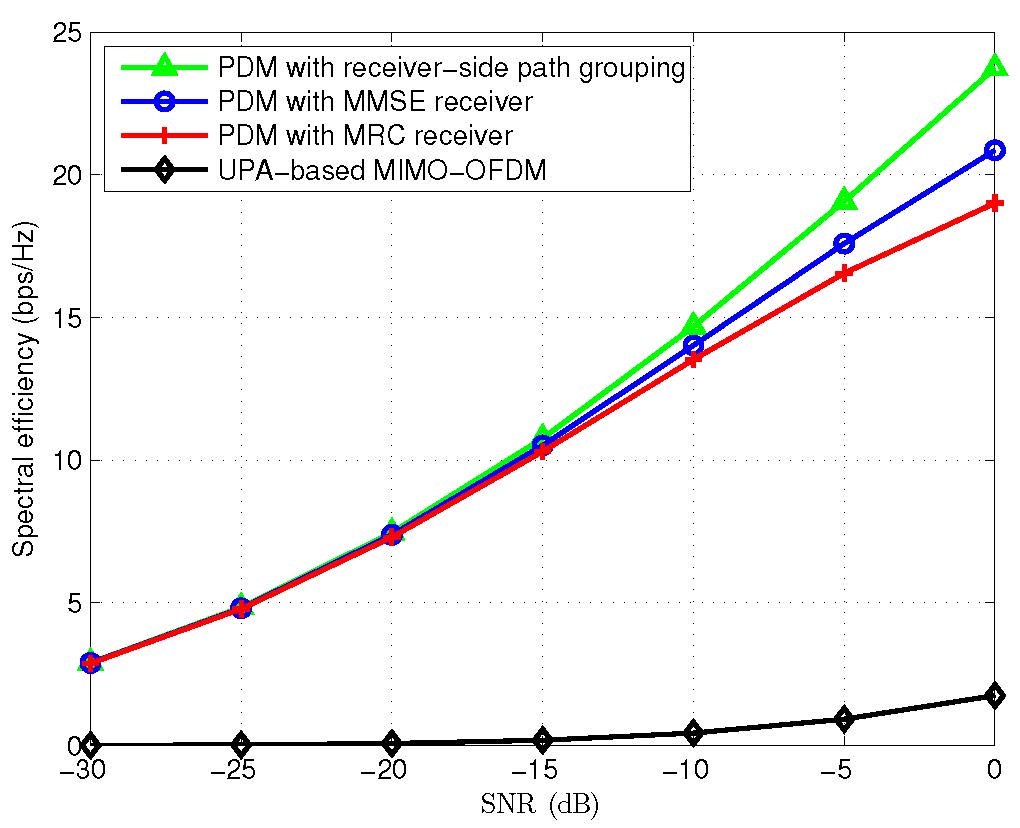
Figure 12: Average spectrum efficiency achieved by various schemes in wide-band mmWave MIMO communication with antenna selection. The number of transmitting/receiving RF chains are $M_{\text{RF}}=Q_{\text{RF}}=6$. AoA angular spread is $\Phi_{R}=150^{\circ}$.

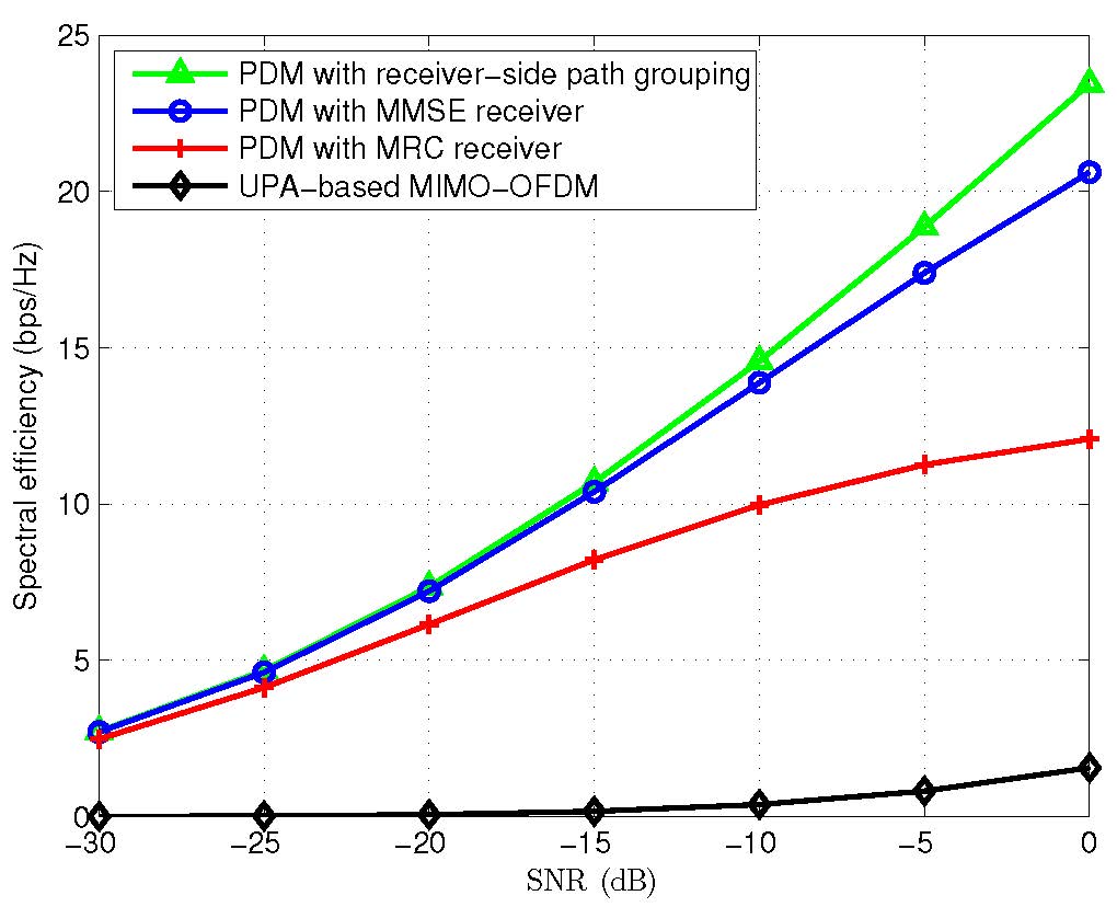
Figure 13: Average spectrum efficiency achieved by various schemes in wide-band mmWave MIMO communication with antenna selection. The number of transmitting/receiving RF chains are $M_{\text{RF}}=Q_{\text{RF}}=6$. AoA angular spread is $\Phi_{R}=10^{\circ}$.

V Conclusion and Future Work

In this paper, we studied the use of lens antenna arrays for mmWave MIMO communications. The array response of the lens antenna array was derived and compared with that of conventional UPA without the lens. We showed that the proposed lens antenna array significantly reduces the signal processing complexity and RF chain cost as compared to the conventional UPA in mmWave MIMO communications, and yet without notable performance degradation. We proposed a new low-complexity MIMO spatial multiplexing technique called PDM, for both narrow-band and wide-band communications. Analytical results showed that the PDM scheme is able to achieve perfect ISI rejection as long as the AoAs or AoDs are sufficiently separated, thanks to the energy focusing capability of the lens antenna. Finally, for cases with insufficient AoA/AoD separations, a simple path grouping technique was proposed for PDM to mitigate inter-path interference more effectively.

There are a number of interesting directions that are worthy of future investigation, which are briefly discussed as follows.

• Elevation AoAs/AoDs: For systems with non-negligible elevation AoAs/AoDs, the array configuration of the lens antenna arrays needs to be refined. In this case, the antenna elements should be generally placed on the focal surface of the EM lens to exploit the elevation angular dimension as well, instead of on the focal arc only as considered in this paper. As a result, the signal multi-paths can be further differentiated with the additional elevation AoA/AoD dimension.

• Multi-User Systems: The PDM for the point-to-point mmWave MIMO communication can be extended to the general path division multiple access (PDMA) for multi-user mmWave systems, by which a number of users with well separated AoAs/AoDs can be simultaneously served with low-complexity and low-cost transceiver designs. The transmission scheduling of users based on their AoAs/AoDs is also worth investigating.

• Channel Estimation: In this paper, we assume perfect channel state information at both the transmitter and receiver, while in practical mmWave systems such knowledge needs to be efficiently obtained via well-designed channel training/estimation/feedback schemes. For mmWave MIMO communications with conventional arrays, channel estimation is a challenging task due to the large-antenna dimension as well as the low SNR before beamforming is applied [14, 16, 21]; whereas with lens antenna arrays, by exploiting its energy focusing as well as the multi-path sparsity of mmWave channels, the effective channel dimension is significantly reduced and the pre-beamforming SNR is greatly enhanced. Therefore, channel knowledge can be obtained far more efficiently as compared to conventional arrays, which deserves further study.

Appendix A Proof of Lemma 1

To derive the array response of the proposed lens antenna array given in Lemma 1, we first present the fundamental principle of operation for EM lenses. EM lenses are fundamentally similar to optical lenses, which are able to alter the propagation directions of the EM rays to achieve energy focusing or beam collimation.

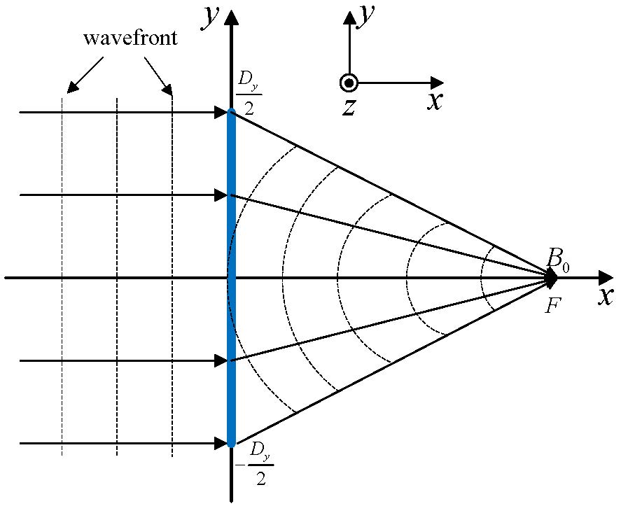
Figure 14: Top view of a planar EM lens placed in the y-z plane with focal point $B_{0}(F,0,0)$ for normal incident plane waves.

Fig. 14 shows a planar EM lens of size $D_{y}\times D_{z}$ placed in the y-z plane and centered at the origin. Denote by $B_{0}$ with coordinate $(F,0,0)$ the focal point of the lens for normal incident plane waves, where $F$ is known as the focal length. The main mechanism to achieve energy focusing at $B_{0}$ is to design the phase shift profile $\Phi(y,z)$, which represents the phase delay provided by the spatial phase shifters (SPS) of the lens at any point $(0,y,z)$ on the lens’s aperture, such that all rays with normal incidence arrive at $B_{0}$ with identical phase for constructive superposition [35]. We thus have

$$\Phi(y,z)+ k_{0}d(y,z,B_{0})=\Phi_{0},$$

$$\forall(y,z)\in\left[-\frac{D_{y}}{2},\frac{D_{y}}{2}\right]\times\left[-\frac{D_{z}}{2},\frac{D_{z}}{2}\right],$$ (45)

where $k_{0}=2\pi/\lambda$ is the free-space wave number of the incident wave, with $\lambda$ denoting the free-space wavelength, $d(y,z,B_{0})=\sqrt{F^{2}+y^{2}+z^{2}}$ is the distance between the point $(0,y,z)$ on the lens’s aperture and the focal point $B_{0}$, and $\Phi_{0}$ is a positive constant denoting the common phase delay from the lens’s input aperture to the focal point $B_{0}$. The phase shift profile is then designed to be

$$\Phi(y,z)=\Phi_{0} -k_{0}\sqrt{F^{2}+y^{2}+z^{2}},$$

$$\forall(y,z)\in\left[-\frac{D_{y}}{2},\frac{D_{y}}{2}\right]\times\left[-\frac{D_{z}}{2},\frac{D_{z}}{2}\right].$$ (46)

As can be seen from (46), due to the different propagation distances from the lens’s aperture to $B_{0}$, the phase shift profile varies across the lens apertures with different $y$ and $z$ values. In general, larger phase delay needs to be provided by the SPS located in the center of the lens than those on the edge.

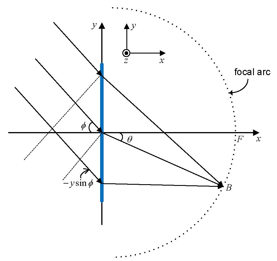
Figure 15: A planar EM lens placed in the y-z plane with oblique incident plane wave of azimuth AoA $\phi$.

With the phase shift profile designed in (46) to achieve focal point $B_{0}$ for normal incident wave, the resulting phase delay from the lens’s input aperture $(0,y,z)$ to an arbitrary point $B(x_{B},y_{B},z_{B})$ is then given by

$$\psi(y,z,B)=\Phi(y,z)+k_{0}d(y,z,B),$$ (47)

where $d(y,z,B)=\sqrt{x_{B}^{2}+(y_{B}-y)^{2}+(z_{B}-z)^{2}}$ denotes the distance from the point $(0,y,z)$ on the lens to point $B$. Of particular interest is the field distribution on the focal arc of the lens, which is defined as the arc on the x-y plane with a distance $F$ from the lens center, as shown in Fig. 15. Let $B(F\cos\theta,-F\sin\theta,0)$ be a point on the focal arc parameterized by angle $\theta\in[-\frac{\pi}{2},\frac{\pi}{2}]$. With (46) and (47), we have

$$\psi(y,z,\theta) =\Phi_{0}-k_{0}\sqrt{F^{2}+y^{2}+z^{2}}+k_{0}\sqrt{F^{2}+y^{2}+z^{2}+2yF\sin\theta}$$ (48)

$$\approx\Phi_{0}+k_{0}y\sin\theta,$$ (49)

where (49) follows from the first-order Taylor approximation and the assumption that $F\gg D_{y},D_{z}$.

Let $s(y,z)$ denote the incident signal arriving at the lens’s input aperture. Due to the linear superposition principle, the resulting signal on the focal arc of the lens can then be expressed as

$$r(\theta) =\int_{-D_{z}/2}^{D_{z}/2}\int_{-D_{y}/2}^{D_{y}/2}s(y,z)e^{-j\psi(y,z,\theta)}dydz$$ (50)

$$=e^{-j\Phi_{0}}D_{z}\int_{-D_{y}/2}^{D_{y}/2}s(y)e^{-j\frac{2\pi}{\lambda}y\sin\theta}dy,\ \theta\in\left[-\frac{\pi}{2},\frac{\pi}{2}\right],$$ (51)

where in (51), we have assumed that $s(y,z)=s(y)$, $\forall(y,z)\in\left[-\frac{D_{y}}{2},\frac{D_{y}}{2}\right]\times\left[-\frac{D_{z}}{2},\frac{D_{z}}{2}\right]$, which is true for uniform incident plane waves with negligible elevation AoAs. For notational convenience, we assume that $\Phi_{0}=2n\pi$ for some integer $n$, so that it can be ignored in (51). Furthermore, by defining

$$\tilde{D}=\frac{D_{y}}{\lambda},\quad\tilde{y}=\frac{y}{\lambda},\quad\tilde{\theta}=\sin(\theta),$$ (52)

the relationship in (51) can be equivalently written as

$$r(\tilde{\theta})=D_{z}\int_{-\tilde{D}/2}^{\tilde{D}/2}\tilde{s}(\tilde{y})e^{-j2\pi\tilde{\theta}\tilde{y}}d\tilde{y},\quad\tilde{\theta}\in[-1,1],$$ (53)

where $\tilde{s}(\tilde{y})$ with $\tilde{y}\in\left[-\tilde{D}/2,\tilde{D}/2\right]$ is a linear scaling of the arriving signal $s(y)$ given by $\tilde{s}(\tilde{y})\triangleq\lambda s(\lambda\tilde{y})$.

It is interesting to observe from (53) that with the spatial phase shifting provided by the EM lens, the resulting signal at the focal arc of the lens can be represented as the Fourier transform of the arriving signal $\tilde{s}(\tilde{y})$ at the lens’s input aperture, with $\tilde{\theta}\in[-1,1]$ and $\tilde{y}\in\left[-\tilde{D}/2,\tilde{D}/2\right]$ in (53) referred to as the spatial frequency and the spatial time, respectively.

For uniform incident plane waves with azimuth AoA $\phi$, or equivalently with spatial frequency $\tilde{\phi}=\sin(\phi)$, as shown in Fig. 15, we have $s(y)=\frac{1}{\lambda\sqrt{D_{y}D_{z}}}x_{0}(\phi)e^{j\frac{2\pi}{\lambda}y\sin(\phi)}$, or equivalently

$$\tilde{s}(\tilde{y})=\frac{1}{\sqrt{D_{y}D_{z}}}x_{0}(\phi)e^{j2\pi\tilde{y}\tilde{\phi}},$$ (54)

where $x_{0}(\phi)$ is the input signal arriving at the lens center with AoA $\phi$, and $\sqrt{D_{y}D_{z}}$ is a normalization factor to ensure that the total power captured by the lens is proportional to its effective aperture $A\triangleq D_{y}D_{z}/\lambda^{2}$. By substituting (54) into (53), we have

$$r(\tilde{\theta})=x_{0}(\phi)\sqrt{A}\mathrm{sinc}\left(\tilde{D}(\tilde{\theta}-\tilde{\phi})\right),\quad\tilde{\theta}\in[-1,1].$$ (55)

It then follows from (55) that the effective lens response on its focal arc for incident plane waves with AoA $\phi$ (or spatial frequency $\tilde{\phi}$) is

$$a_{\tilde{\theta}}(\phi)=\sqrt{A}\mathrm{sinc}(\tilde{D}(\tilde{\theta}-\tilde{\phi})),\ \tilde{\theta}\in[-1,1].$$ (56)

For the lens antenna array with the $m$th element located at position $B_{m}(F\cos(\theta_{m}),-F\sin(\theta_{m}),0)$, it follows from (56) that the array response can be expressed as

$$a_{m}(\phi)=\sqrt{A}\mathrm{sinc}\left(\tilde{D}(\sin\theta_{m}-\sin\phi)\right),\ \forall m.$$ (57)

In particular, with the critical antenna spacing specified in (1), the array response in (57) reduces to

$$a_{m}(\phi)=\sqrt{A}\mathrm{sinc}\left(m-\tilde{D}\sin\phi\right),\ \forall m.$$ (58)

This completes the proof of Lemma 1.

References

- [1] J. G. Andrews, S. Buzzi, W. Choi, S. V. Hanly, A. Lozano, A. C. K. Soong, and J. C. Zhang, “What will 5G be?” IEEE J. Sel. Areas Commun., vol. 32, no. 6, pp. 1065–1082, Jun. 2014.
- [2] F. Boccardi, R. W. Heath Jr, A. Lozano, T. L. Marzetta, and P. Popovski, “Five disruptive technology directions for 5G,” IEEE Commun. Mag., vol. 52, no. 2, pp. 74–80, Feb. 2014.
- [3] Z. Pi and F. Khan, “An introduction to millimeter-wave mobile broadband systems,” IEEE Commun. Mag., vol. 49, no. 6, pp. 101–107, Jun. 2011.
- [4] T. S. Rappaport, S. Sun, R. Mayzus, H. Zhao, Y. Azar, K. Wang, G. N. Wong, J. K. Schulz, M. Samimi, and F. Gutierrez, “Millimeter wave mobile communications for 5G cellular: it will work!” IEEE Access, vol. 1, pp. 335–349, May 2013.
- [5] S. Rangan, T. S. Rappaport, and E. Erkip, “Millimeter-wave cellular wireless networks: potentials and challenges,” Proceedings of the IEEE, vol. 102, no. 3, pp. 366–385, Mar. 2014.
- [6] T. S. Rappaport, R. W. Heath Jr, R. C. Daniels, and J. N. Murdock, Millimeter wave wireless communications. Prentice Hall, 2014.
- [7] T. Baykas, C. S. Sum, Z. Lan, J. Wang, M. A. Rahman, H. Harada, and S. Kato, “IEEE 802.15.3c: the first IEEE wireless standard for data rates over 1Gb/s,” IEEE Commun. Mag., vol. 49, no. 7, pp. 114–121, Jul. 2011.
- [8] T. Nitsche, C. Cordeiro, A. B. Flores, E. W. Knightly, E. Perahia, and J. C. Widmer, “IEEE 802.11ad: directional 60 GHz communication for multi-Gigabit-per-second Wi-Fi,” IEEE Commun. Mag., vol. 52, no. 12, pp. 132–141, Dec. 2014.
- [9] M. R. Akdeniz, Y. Liu, M. K. Samimi, S. Sun, S. Rangan, T. S. Rappaport, and E. Erkip, “Millimeter wave channel modeling and cellular capacity evalutation,” IEEE J. Sel. Areas Commun., vol. 32, no. 6, pp. 1164–1179, Jun. 2014.
- [10] W. Roh, J. Y. Seo, J. Park, B. Lee, J. Lee, Y. Kim, J. Cho, K. Cheun, and F. Aryanfar, “Millimeter-wave beamforming as an enabling technology for 5G cellular communications: theoretical feasibility and prototype results,” IEEE Commun. Mag., vol. 52, no. 2, pp. 106–113, Feb. 2014.
- [11] A. Alkhateeb, J. Mo, N. G. Prelcic, and R. W. Heath Jr, “MIMO precoding and combining solutions for millimeter-wave systems,” IEEE Commun. Mag., vol. 52, no. 12, pp. 122–131, Dec. 2014.
- [12] S. Sun, T. S. Rappaport, R. W. Heath Jr, A. Nix, and S. Rangan, “MIMO for millimeter-wave wireless communications: beamforming, spatial multiplexing, or both?” IEEE Commun. Mag., vol. 52, no. 12, pp. 110–121, Dec. 2014.
- [13] A. Ghosh, T. A. Thomas, M. C. Cudak, R. Ratasuk, P. Moorut, F. Vook, T. S. Rappaport, G. MacCartney, S. Shu, and N. Shuai, “Millimeter-wave enhanced local area systems: a high-data-rate approach for future wireless networks,” IEEE J. Sel. Areas Commun., vol. 32, no. 6, pp. 1152–1163, Jun. 2014.
- [14] J. Wang, Z. Lan, C. W. Pyo, T. Baykas, C. S. Sum, M. A. Rahman, J. Gao, R. Funada, F. Kojima, H. Harada, and S. Kato, “Beam codebook based beamforming protocol for multi-gbps millimeter-wave WPAN systems,” IEEE J. Sel. Areas Commun., vol. 27, no. 8, pp. 1390–1399, Oct. 2009.
- [15] F. Gholam, J. Via, and I. Santamaria, “Beamforming design for simplified analog antenna combining architectures,” IEEE Trans. Veh. Technol., vol. 60, no. 5, pp. 2373–2378, Jun. 2011.
- [16] S. Hur, T. Kim, D. J. Love, J. V. Krogmeier, T. A. Thomas, and A. Ghosh, “Millimeter wave beamforming for wireless backhaul and access in small cell networks,” IEEE Trans. Commun., vol. 61, no. 10, pp. 4391–4403, Oct. 2013.
- [17] X. Zhang, A. F. Molish, and S. Y. Kung, “Variable-phase-shift-based RF-baseband codesign for MIMO antenna selection,” IEEE Trans. Signal Process., vol. 53, no. 11, pp. 4091–4103, Nov. 2005.
- [18] V. Venkateswaran and A. J. van der Veen, “Analog beamforming in MIMO communications with phase shift networks and online channel estimation,” IEEE Trans. Signal Process., vol. 58, no. 8, pp. 4131–4143, Aug. 2010.
- [19] O. E. Ayach, S. Rajagopal, S. Abu-Surra, Z. Pi, and R. W. Heath Jr, “Spatially sparse precoding in millimeter wave MIMO systems,” IEEE Trans. Wireless Commun., vol. 13, no. 3, pp. 1499–1513, Mar. 2013.
- [20] T. Kim, J. Park, J. Y. Seol, S. Jeong, J. Cho, and W. Roh, “Tens of Gbps support with mmWave beamforming systems for next generation communications,” IEEE Global Telecom. Conf. (GLOBECOM), pp. 3685–3690, Dec. 9-13, 2013.
- [21] A. Alkhateeb, O. E. Ayach, R. Leus, and R. W. Heath Jr, “Channel estimation and hybrid precoding for millimeter wave cellular systems,” IEEE J. Sel. Topics Signal Process., vol. 8, no. 5, pp. 831–846, Oct. 2014.
- [22] A. Alkhateeb, G. Leus, and R. W. Heath Jr, “Limited feedback hybrid precoding for multi-user millimeter wave systems,” 2014, submitted to IEEE Trans. Wireless Commun., arXiv preprint arXiv:1409.5162.
- [23] R. M. Rial, C. Rusu, A. Alkhateeb, N. G. Prelcic, and R. W. Heath Jr, “Channel estimation and hybrid combining for mmWave: phase shifters or switches?” in Proc. Inf. Theory Applications Workshop (ITA), Feb. 2015.
- [24] S. Sanayei and A. Nosratinia, “Antenna selection in MIMO systems,” IEEE Commun. Mag., pp. 68–73, Oct. 2004.
- [25] A. F. Molish and M. Z. Win, “MIMO systems with antenna selection,” IEEE Microw. Mag., pp. 46–56, Mar. 2004.
- [26] A. Sayeed and N. Behdad, “Continuous aperture phased MIMO: basic theory and applications,” in Proc. 48th Annu. Allerton Conf. on Commun., Control, and Computing, Sep. 2010, pp. 1196–1203.
- [27] J. Brady, N. Behdad, and A. M. Sayeed, “Beamspace MIMO for millimeter-wave communications: system architecture, modeling, analysis, and measurements,” IEEE Trans. Antennas Propag., vol. 61, no. 7, pp. 3814–3827, Jul. 2013.
- [28] Y. Zeng, R. Zhang, and Z.-N. Chen, “Electromagnetic lens-focusing antenna enabled massive MIMO,” in IEEE Int. Conf. Commun. in China (ICCC), Aug. 2013.
- [29] ——, “Electromagnetic lens-focusing antenna enabled massive MIMO: performance improvement and cost reduction,” IEEE J. Sel. Areas Commun., vol. 32, no. 6, pp. 1194–1206, Jun. 2014.
- [30] T. Kwon, Y. G. Lim, and C. B. Chae, “Limited channel feedback for RF lens antenna based massive MIMO systems,” in Proc. IEEE Int. Conf. Computing, Networking and Communications (ICNC), Feb. 2015.
- [31] B. Bares, R. Sauleau, L. L. Coq, and K. Mahdjoubi, “A new accurate design method for millimeter-wave homogeneous dielectric substrate lens antennas of arbitrary shape,” IEEE Trans. Antennas Propag., vol. 53, no. 3, pp. 1069–1082, Mar. 2005.
- [32] P.-Y. Lau, Z.-N. Chen, and X.-M. Qing, “Electromagnetic field distribution of lens antennas,” in Proc. Asia-Pacific Conf. Antennas and Propag., Aug. 2013.
- [33] Z. Popovic and A. Mortazawi, “Quasi-optical transmit/receive front ends,” IEEE Trans. Microwave Th. Techn., vol. 46, no. 11, pp. 1964–1975, Nov. 1998.
- [34] Z. P. S. Hollung and A. Cox, “A bi-directional quasi-optical lens amplifier,” IEEE Trans. Microwave Th. Techn., vol. 45, no. 12, pp. 1964–1975, Dec. 1997.
- [35] M. A. Al-Joumayly and N. Behdad, “Wideband planar microwave lenses using sub-wavelenth spatiall phase shifters,” IEEE Trans. Antennas Propag., vol. 59, no. 12, pp. 4542–4552, Dec. 2011.
- [36] M. Li, M. A. Al-Joumayly, and N. Behdad, “Broadband true-time-delay microwave lenses based on miniaturized element frequency selective surfaces,” IEEE Trans. Antennas Propag., vol. 61, no. 3, pp. 1166–1179, Mar. 2013.
- [37] T. L. Marzetta, “Noncooperative cellular wireless with unlimited numbers of base station antennas,” IEEE Trans. Wireless Commun., vol. 9, no. 11, pp. 3590–3600, Nov. 2010.
- [38] F. Rusek, D. Persson, B. K. Lau, E. G. Larsson, T. L. Marzetta, O. Edfors, and F. Tufvesson, “Scaling up MIMO: opportunities and challenges with very large arrays,” IEEE Signal Process. Mag., vol. 30, no. 1, pp. 40–60, Jan. 2013.
- [39] L. Lu, G. Y. Li, A. L. Swindlehurst, A. Ashikhin, and R. Zhang, “An overview of massive MIMO: benefits and challenges,” IEEE J. Sel. Topics Signal Process., vol. 8, no. 5, pp. 742–758, Oct. 2014.
- [40] A. Goldsmith, Wireless Communications. Cambridge University Press, 2005.
- [41] H. Yin, D. Gesbert, M. Filippou, and Y. Liu, “A coordinated approach to channel estimation in large-scale multiple-antenna systems,” IEEE J. Sel. Areas Commun., vol. 31, no. 2, pp. 264–273, Feb. 2013.
- [42] A. Adhikary, J. Nam, J. Y. Ahn, and G. Caire, “Joint spatial division and multiplexing-the large-scale array regime,” IEEE Trans. Inf. Theory, vol. 59, no. 10, pp. 6441–6463, Oct. 2013.
- [43] A. Adhikary, E. A. Safadi, M. K. Samimi, R. Wang, G. Caire, T. S. Rappaport, and A. F. Molish, “Joint spatial division and multiplexing for mm-wave channels,” IEEE J. Sel. Areas Commun., vol. 32, no. 6, pp. 1239–1255, Jun. 2014.
- [44] C. Sun, X. Gao, S. Jin, M. Matthaiou, Z. Ding, and C. Xiao, “Beam division multiple access transmission for massive MIMO communications,” IEEE Trans. Commun., vol. 63, no. 6, pp. 2170–2184, Jun. 2015.
- [45] R. B. Ertel, P. Cardieri, K. W. Sowerby, T. S. Rappaport, and J. H. Reed, “Overview of spatial channel models for antenna array communication systems,” IEEE Personal Commun., vol. 5, no. 1, pp. 10–22, Feb. 1998.
- [46] M. Brand, “Fast low-rank modifications of the thin singular value decomposition,” Elsevier linear algebra and its applications, pp. 20–30, 2006.
- [47] S. M. Kay, Fundumentals of Statistical Signal Processing: Estimation Theory. New Jersey: Prentice-Hall, 1993.