Path-Fault-Tolerant Approximate
Shortest-Path Trees

Abstract

Let $G=(V,E)$ be an $n$-nodes non-negatively real-weighted undirected graph. In this paper we show how to enrich a single-source shortest-path tree (SPT) of $G$ with a sparse set of auxiliary edges selected from $E$, in order to create a structure which tolerates effectively a path failure in the SPT. This consists of a simultaneous fault of a set $F$ of at most $f$ adjacent edges along a shortest path emanating from the source, and it is recognized as one of the most frequent disruption in an SPT. We show that, for any integer parameter $k\geq 1$, it is possible to provide a very sparse (i.e., of size $O(kn\cdot f^{1+1/k})$) auxiliary structure that carefully approximates (i.e., within a stretch factor of $(2k-1)(2|F|+1)$) the true shortest paths from the source during the lifetime of the failure. Moreover, we show that our construction can be further refined to get a stretch factor of $3$ and a size of $O(n\log n)$ for the special case $f=2$, and that it can be converted into a very efficient approximate-distance sensitivity oracle, that allows to quickly (even in optimal time, if $k=1$) reconstruct the shortest paths (w.r.t. our structure) from the source after a path failure, thus permitting to perform promptly the needed rerouting operations. Our structure compares favorably with previous known solutions, as we discuss in the paper, and moreover it is also very effective in practice, as we assess through a large set of experiments.

1 Introduction

Broadcasting data from a source node to every other node of a network is one of the most basic communication primitives in modern networked applications. Given the widespread diffusion of such applications, in the recent past, there has been an increasing demand for more and more efficient, i.e. scalable and reliable, methods to implement this fundamental feature.

The natural solution is that of modeling the network as a graph (nodes as vertices and links as edges) and building a (fast and compact) structure to be used to transmit the data. In particular, the most common approach of this kind is that of computing a shortest-path tree (SPT), rooted at the desired source node, of such graph.

However, the SPT, as any tree-based topology, is prone to unpredictable events that might occur in practice, such as failures of nodes and/or links. Therefore, the use of SPTs might result in a high sensitivity to malfunctioning, which unavoidably causes the undesired effect of disconnecting sets of nodes from the source and thus the interruption of the broadcasting service.

Therefore, a general approach to cope with this scenario is to make the SPT fault-tolerant against a given number of simultaneous component failures, by adding to it a set of suitably selected edges from the underlying graph, so that the resulting structure will remain connected w.r.t. the source. In other words, the selected edges can be used to build up alternative paths from the root, each one of them in replacement of a corresponding original shortest path which was affected by the failure. However, if these paths are constrained to be shortest, then it can be easily seen that for a non-negatively real weighted and undirected graph of $n$ nodes and $m$ edges, this may require as much as $\Theta(m)$ additional edges, also in the case in which $m=\Theta(n^{2})$. In other words, the set-up costs of the strengthened network may become unaffordable.

Thus, a reasonable compromise is that of building sparse and fault-tolerant structure which approximates the shortest paths from the source, i.e., that contains paths which are guaranteed to be longer than the corresponding shortest paths by at most a given stretch factor, for any possible edge/vertex failure that has to be handled. In this way, the obtained structure can be revised as a 2-level communication network: a first primary level, i.e., the SPT, which is used when all the components are operational, and an auxiliary level which comes into play as soon as a component undergoes a failure.

In this paper, we show that an efficient structure of this sort exists for a prominent class of failures in an SPT, namely those involving a set of adjacent edges along a shortest path emanating from the source of the SPT. Our study is motivated by several applications, such as, for instance, traffic engineering in optical networks or path-congestion management in road-networks, where failures in the above form often affect the SPT [5, 11, 19]. For this kind of failure, also known as a path failure, we show that it is possible not only to obtain resilient sparse structures, but also that these can be pre-computed efficiently, and that they can return quickly the auxiliary network level.

1.1 Related Work

In the recent past, many efforts have been dedicated to devising single and multiple edge/vertex fault-tolerant structures. More formally, let $r$ denote a distinguished source vertex of a non-negatively real-weighted and undirected graph $G=(V(G),E(G))$, with $n$ nodes and $m$ edges. We say that a spanning subgraph $H$ of $G$ is an Edge/Vertex-fault-tolerant $\alpha$-Approximate SPT (in short, $\alpha$-E/VASPT), with $\alpha>1$, if it satisfies the following condition: For each edge $e\in E(G)$ (resp., vertex $v\in V(G)$), all the distances from $r$ in the subgraph $H-e$, i.e., $H$ deprived of edge $e$ (resp., the subgraph $H-v$, i.e., $H$ deprived of vertex $v$ and all its incident edges) are $\alpha$-stretched (i.e., at most $\alpha$ times longer) w.r.t. the corresponding distances in $G-e$ (resp., $G-v$).

An early work on the matter is [20], where the authors showed that by adding at most $n-1$ edges to the SPT, a 3-EASPT can be obtained. This was shown to be very useful in order to compute a recovery scheme needing only one backup routing table at each node [18]. In [15], the authors showed instead how to build a 1-EASPT in $\widetilde{O}(mn)$ time. Notice that, a 1-EASPT contains exact replacement paths from the source, but of course its size might be $\Theta(n^{2})$ if $G$ is dense. Then, in [2], Baswana and Khanna devised a $3$-VASPT of size $O(n\log n)$. Later on, a significant improvement to this result was provided in [6], where the authors showed the existence of a $(1+\varepsilon)$-E/VASPT, for any $\varepsilon>0$, of size $O(\frac{n\log n}{\varepsilon^{2}})$.

Concerning unweighted graphs, in [2] the authors give a $(1+\varepsilon)$-VABFS (where BFS stands for breadth-first search tree) of size $O(\frac{n}{\varepsilon^{3}}+n\log n)$ (actually, such a size can be easily reduced to $O(\frac{n}{\varepsilon^{3}})$). Then, Parter and Peleg in [21] present a set of lower and upper bounds to the size of a $(\alpha,\beta)$-EABFS, namely a structure for which the length of a path is stretched by at most a factor of $\alpha$, plus an additive term of $\beta$. More precisely, they construct a $(1,4)$-EABFS of size $O(n^{4/3})$. Moreover, assuming at most $f=O(1)$ edge failures can take place, they show the existence of a $(3(f+1),(f+1)\log n)$-EABFS of size $O(fn)$. This was improving onto the general fault-tolerant spanner construction given in [9], which, for weighted graphs and for any integer parameter $k\geq 1$, is resilient to up to $f$ edge failures with stretch factor of $2k-1$ and size $O(f\cdot n^{1+1/k})$.

On the other hand, concerning approximate-distance sensitivity oracles (simply $\alpha$-oracles in the following, where $\alpha$ denotes the guaranteed approximation ratio w.r.t. true distances), researchers aimed at computing, with a low preprocessing time, a compact data structure able to quickly answer to some distance query following an edge/vertex failure. The vast literature dates back to the work [23] of Thorup and Zwick, who showed that, for any integer $k\geq 1$, any undirected graph with non-negative edge weights can be preprocessed in $O(km\cdot n^{1/k})$ time to build a $(2k-1)$-oracle of size $O(k\cdot n^{1+1/k})$, answering in $O(k)$ time to a post-failure distance query, recently reduced to $O(1)$ time in [8]. Due to the long-standing girth conjecture of Erdős [13], this is essentially optimal. Concerning the failure of a set $F$ of at most $f$ edges, in [10] the authors built, for any integer $k\geq 1$, a $(8k-2)(f+1)$-oracle of size $O(fk\cdot n^{1+1/k}\log(nW))$, where $W$ is the ratio of the maximum to the minimum edge weight in $G$, and with a query time of $\widetilde{O}(|F|\cdot\log\log d)$, where $d$ is the actual distance between the queried pair of nodes in $G-F$. As far as SPT oracles (i.e., returning distances/paths only from a source node) are concerned, in [2] it is shown how to build in $O(m\log n+n\log^{2}n)$ time an SPT oracle of size $O(n\log n)$, that for any single-vertex-failure returns a 3-stretched replacement path in time proportional to the path’s size. Finally, for directed graphs with integer positive edge weights bounded by $M$, in [14] the authors show how to build in $\widetilde{O}(Mn^{\omega})$ time and $\Theta(n^{2})$ space a randomized single-edge-failure SPT oracle returning exact distances in $O(1)$ time, where $\omega<2.373$ denotes the matrix multiplication exponent.

1.2 Our Results

In this paper, we consider the specific, yet interesting, problem of making a SPT resilient to the failure of any sub-path of size (i.e., number of edges) at most $f\geq 1$ emanating from its source.

More in details, let $F$ be a set of cascading edges of a given SPT, where $0<|F|\leq f$. We say that a spanning subgraph $H$ of $G$ is a Path-Fault-Tolerant $\alpha$-Approximate SPT (in short, $\alpha$-PASPT), with $\alpha\geq 1$, if, for each vertex $z\in V(G)$, the following inequality holds: $d_{H-F}(z)\leq\alpha\cdot d_{G-F}(z)$, where $d_{G-F}(z)$ (resp., $d_{H-F}(z)$) denotes the distance from $r$ to $z$ in $G-F$ (resp., $H-F$). For any integer parameter $k\geq 1$, we can provide the following results:

• We give an algorithm for computing, in $O(n\cdot(m+f^{2}))$ time, a $(2k-1)(2|F|+1)$-PASPT containing $O(kn\cdot f^{1+\frac{1}{k}})$ edges;

• We give an algorithm for computing, in $O(n\cdot(m+f^{2}))$ time, an oracle of size $O(kn\cdot f^{1+\frac{1}{k}})$ which is able to return: (i) a $(2k-1)(2|F|+1)$-approximate distance in $G-F$ between $r$ and a generic vertex $z$ in $O(k)$ time; (ii) the associated path in $O(k+f+\ell)$ time, where $\ell$ is the number of its edges; if $k=1$, this can be further reduced to $O(\ell)$ time.

Concerning the former result, it compares favorably with both the aforementioned general fault-tolerant spanner constructions given in [9], and the unweighted EABFS provided in [21], while concerning instead the latter result, it compares favorably with the fault-tolerant oracle given in [10]. For the sake of fairness, we remind that all these structures were thought to cope with edge failures arbitrarily spread across $G$, though.

Besides that, we also analyze in detail the special case when at most $f=2$ failures of cascading edges can occur, for which we are able to achieve a significantly better stretch factor. More precisely, we design: (i) an algorithm for computing, in $O(n\cdot(m+n\log n))$ time, a 3-PASPT containing $O(n\log n)$ edges; (ii) an algorithm for computing, in $O(n\cdot(m+n\log n))$ time, an oracle of size $O(n\log n)$ which is able to return a $3$-approximate distance in $G-F$ between $r$ and a generic vertex $z$ in constant time, and the associated path in a time proportional to the number of its edges. Some of the proofs related to these latter results will be given in the appendix.

Finally, we provide an experimental evaluation of the proposed structures, to assess their performance in practice w.r.t. both size and quality of the stretch.

2 Notation

In what follows, we give our notation for the considered problem. We are given a non-negatively real-weighted, undirected graph $G=(V(G),E(G))$ with $|V(G)|=n$ vertices and $|E(G)|=m$ edges. We denote by $w_{G}(e)$ or $w_{G}(u,v)$ the weight of the edge $e=(u,v)\in E(G)$. Given an edge $e=(u,v)$, we denote by $G-e$ or $G-(u,v)$ the graph obtained from $G$ by removing the edge $e$. Similarly, for a set $F$ of edges, $G-F$ denotes the graph obtained from $G$ by removing the edges in $F$. Furthermore, given a vertex $v\in V(G)$, we denote by $G-v$ the graph obtained from $G$ by removing vertex $v$ and all its incident edges. Given a graph $G$, we call $\pi_{G}(x,y)$ a shortest path between two vertices $x,y\in V(G)$, $d_{G}(x,y)$ its weighted length (i.e., the distance from $x$ to $y$ in $G$), $T_{G}(r)$ a shortest path tree (SPT) of $G$ rooted at a certain distinguished source vertex $r$. Moreover, we denote by $T_{G}(r,x)$ the subtree of $T_{G}(r)$ rooted at vertex $x$. Whenever the graph $G$ and/or the source vertex $r$ are clear from the context, we might omit them, i.e., we write $\pi(u)$ and $d(u)$ instead of $\pi_{G}(r,u)$ and $d_{G}(r,u)$, respectively. When considering an edge $(x,y)$ of an SPT, we assume $x$ and $y$ to be the closest and the furthest endpoints from $r$, respectively. Furthermore, if $P$ is a path from $x$ to $y$ and $Q$ is a path from $y$ to $z$, with $x,y,z\in V(G)$, we denote by $P\circ Q$ the path from $x$ to $z$ obtained by concatenating $P$ and $Q$. We also denote by $w(P)$ the total weight of the edges in $P$.

For the sake of simplicity we consider only edge weights that are strictly positive. However, our entire analysis also extends to non-negative weights. Throughout the rest of the paper, we assume that, when multiple shortest paths exist, ties are broken in a consistent manner. In particular we fix an SPT $T=T_{G}(r)$ of $G$ and, given a graph $H\subseteq G$ and $x,y\in V(H)$, whenever we compute the path $\pi_{H}(x,y)$ and ties arise, we prefer edges in $E(T)$.

A path between any two vertices $u,v\in V(G)$ is said to be an $\alpha$–approximate shortest path if its length is at most $\alpha$ times the length of the shortest path between $u$ and $v$ in $G$. For the sake of simplicity, we assume that, if a set of at most $f$ edge failures has to be handled, the original graph is $(f+1)$–edge connected. Indeed, if this is not the case, we can guarantee the $(f+1)$–edge connectivity by adding at most $O(nf)$ edges of weight $+\infty$ to $G$. Notice that this is not actually needed by any of the proposed algorithms.

3 Our PASPT Structure and the Corresponding Oracle

In what follows, we give a high-level description of our algorithm for computing a $(2|F|+1)$-PASPT, namely $H$ (see Algorithm 1), where $|F|\leq f$. We define the level $\ell(v)$ of a vertex $v\in V(G)$ to be the hop-distance between $r$ and $v$ in $T=T_{G}(r)$, i.e., the number of edges of the unique path from $r$ to $v$ in $T$. Note that, when a failure of $|F|$ consecutive edges occurs on a shortest path, $T$ will be broken into a forest $\mathcal{C}$ of $|F|+1$ subtrees. We consider these subtrees as rooted according to $T$, i.e., each tree $T_{i}$ is rooted at vertex $r_{i}$ that minimizes $\ell(r_{i})$.

Roughly speaking, the algorithm considers all possible path failures $F^{*}$ of $f$ vertices by fixing the deepest endpoint $v$ of the failing path. It then reconnects the resulting $f+1$ subtrees of $G-F^{*}$ by selecting at most $O(f^{2})$ edges into a graph $U$, one for each couple of trees $T^{*}_{i},T^{*}_{j}$ of the forest $G-F$. These edges are either directly added to the structure $H$ or they are first sparsified into a graph $U^{\prime}$ by using a suitable multiplicative $(2k-1)$-spanner, so that only $kf^{1+\frac{1}{k}}$ of them are added to $H$.

In particular, it is known that, given an $n$-vertex graph and an integer $k\geq 1$, both a $(2k-1)$–spanner and a $(2k-1)$–approximate distance oracle of size $O(kn^{1+\frac{1}{k}})$ can be built in $O(n^{2})$ time. The oracle can report an approximate distance between two vertices in $O(k)$ time, and the corresponding approximate shortest path in time proportional to the number of its edges. For further details we refer the reader to [3, 4, 22]. Recently, it has been shown in [8] that a randomized $(2k-1)$–approximate distance oracle of expected size $O(kn^{1+\frac{1}{k}})$ can be built, so that answering a distance query requires only constant time. In what follows, however, we only describe results which are based on deterministic construction and provide a worst case guarantee on the size of the resulting structures.

Input : A graph $G$, $r\in V(G)$, an SPT $T=T_{G}(r)$, an integer $f$

Output : A $(2|F|+1)$-PASPT of $G$ rooted at $r$

1 $H\leftarrow T=T_{G}(r)$

2 foreach $v\in V(G)$  do

3       Let $\langle r=z_{0},z_{1},\dots,z_{\ell}(v)\rangle$ be the path from $r$ to $v$ in $T$

       // $F^{*}$ contains last $\min\{f,\ell(v)\}$ edges of the path

4       Let $F^{*}=\{(z_{i-1},z_{i}):i>\ell(v)-\min\{\ell(v),f\}\}$

5       Let $\mathcal{C}^{*}=\{T^{*}_{1},T^{*}_{2},\dots\}$ be the set of connected components of $T-F^{*}$

       // Build an auxiliary graph $U$ associated with $v$

6       $U\leftarrow(\{r^{*}_{i}\,:r^{*}_{i}\mbox{ is the root of }T^{*}_{i}\},\emptyset)$

7       foreach $T^{*}_{i},T^{*}_{j}\in\mathcal{C}^{*}\,:\,T^{*}_{i}\neq T^{*}_{j}$ do

8             Let $E_{i,j}=\{(u,v)\in E(G)\setminus F^{*}:u\in V(T^{*}_{i}),v\in V(T^{*}_{j})\}$

9             $(x^{\prime},y^{\prime})\leftarrow\underset{(x,y)\in E_{i,j}}{\arg\min}\{d_{T}(r^{*}_{i},x)+w_{G}(x,y)+d_{T}(y,r^{*}_{j})\}$

             // We say that $(x^{\prime},y^{\prime})\in E(G)$ is associated to $(r^{*}_{i},r^{*}_{j})\in E(U)$

10             $E(U)\leftarrow E(U)\cup\{(r^{*}_{i},r^{*}_{j})\}$

11             $w_{U}(r^{*}_{i},r^{*}_{j})=d_{T}(r^{*}_{i},x^{\prime})+w_{G}(x^{\prime},y^{\prime})+d_{T}(x^{\prime},r^{*}_{j})$

12            

      // Optional step, executed only if $k\neq 1$. Otherwise, let $U^{\prime}=U$.

13       $U^{\prime}\leftarrow$ Compute a $(2k-1)$-spanner of $U$

14       $E(H)\leftarrow E(H)\cup E(U^{\prime})$

15      

return $H$

Algorithm 1 Algorithm for building a $(2|F|+1)$-PASPT. Notice that an optional integer parameter $k\geq 1$ is used. By default we set $k=1$.

We start by bounding the running time of Algorithm 1:

Lemma 1

Algorithm 1 requires $O(n(m+f^{2}))$ time.

Proof

Notice that the loop in line 1 considers each vertex of $G$ at most once. We bound the time required by each iteration. For each vertex $v$ a complete auxiliary graph $U$ of $O(f)$ vertices is built. Moreover, the weights of all the edges of $U$ can be computed in $O(m)$ time by scanning all the edges of $E(G)\setminus F^{*}$ while keeping track, for each pair of vertices $r^{*}_{i},r^{*}_{j}\in V(U)$, of the minimum value of the formula in line 1. Finally, the optional spanner construction invoked by line 1 requires $O(f^{2})$ time. This concludes the proof.

We now bound the size of the returned structure:

Lemma 2

The structure $H$ returned by Algorithm 1 contains $O(kn\cdot f^{1+\frac{1}{k}})$ edges.

Proof

At the beginning of the algorithm, $H$ coincides with $T=T_{G}(r)$, so $|E(H)|=O(n)$. Therefore, we only need to bound the number of edges added to $H$ during the execution of the algorithm. Notice that, for each vertex $v\in V(G)$, Algorithm 1 considers at most $f+1$ connected components of $\mathcal{C^{*}}$. For each pair of components, at most one edge is added to $U$, hence $|E(U)|=O(f^{2})$. Either $k=1$ and $U^{\prime}=U$ or $k>1$ and $U^{\prime}$ is a $(2k-1)$–spanner of $U$. In both cases we have $|U^{\prime}|=O(k|U|^{1+\frac{1}{k}})=O(kf^{1+\frac{1}{k}})$. As only the edges of $U^{\prime}$ gets added to $H$, the claim follows.

We now upper-bound the distortion provided by the structure $H$. For the sake of clarity, we first discuss the case where the step of line 1 of Algorithm 1 is omitted, i.e., we simply set $k=1$ and $U^{\prime}=U$. At the end of this section we will argue about the general case.

For each path failure $F$ of $|F|\leq f$ edges, and for each target vertex $t$, we will consider a suitable path $P$ in $G-F$, whose length is at most $(2|F|+1)$ times the distance $d_{G-F}(t)$. Then, since $P$ might not be entirely contained in $H-F$, we will show that its length must be an upper bound to the length a path $Q$ in $H-F$ between $r$ an $t$, and hence to $d_{H-F}(t)$.

We first discuss how $P$ is defined: consider the forest $\mathcal{C}$ of the connected components of $T-F$. Let $\pi=\pi_{G-F}(r)$, let $r_{0}=r$, and let $t_{0}$ be the last vertex of $\pi$ belonging to $T_{0}$. W.l.o.g., we assume $t\not\in V(T_{0})$, as otherwise we have $d_{H-F}(t)=d_{G-F}(t)$. Moreover, we call $(t_{0},s_{1})$ the edge following vertex $t_{0}$ in $\pi$.

Initially, we set $P_{0}=\pi_{T}(s,t_{0})\circ(t_{0},s_{1})$ and $i=1$. We proceed iteratively: Let $T_{i}$ be the subtree of $C$ which contains $s_{i}$ and let $t_{i}$ be the last vertex of $\pi$ such that $t_{i}$ belongs to $T_{i}$, i.e., $t_{i}$ is in the same subtree as $s_{i}$ (notice that, it may be that $s_{i}=t_{i})$. Call $r_{i}$ the root of $T_{i}$. If $t_{i}=t$ we set $P=P_{i-1}\circ\pi_{T}(s_{i},r_{i})\circ\pi_{T}(r_{i},t_{i})$, and we are done. Otherwise, let $(t_{i},s_{i+1})$ be the edge following $t_{i}$ in $\pi$. We set $P_{i}=P_{i-1}\circ\pi_{T}(s_{i},r_{i})\circ\pi_{T}(r_{i},t_{i})\circ(t_{i},s_{i+1})$, we increment $i$ by one, and we repeat the whole procedure. Figure 1 shows an example of such a path $P$. Let $h$ be the final value of $i$, at the end of this procedure, so that $t=t_{h}\in V(T_{h})$.

Figure 1: Example of construction of $P$. The path $P$ is shown in bold, while the path $\pi$ is composed of both the light subpaths and of the bold edges with endpoint in different subtrees. In this example $P$ traverses $4$ subtrees and hence $h=3$.

Notice that, by construction, the path $P$ does not contain any failed edge. We now argue that the length $w(P)$ of $P$, is always at most $(2|F|+1)$ times the distance $d_{G-F}(t)$.

Lemma 3

$d_{P}(t)\leq(2|F|+1)\cdot d_{G-F}(t)$, for every $t\in V(G)$.

Proof

We proceed by showing, by induction on $i$, that $d_{P}(t_{i})\leq(2i+1)\cdot d_{G-F}(t_{i})$. The claim follows since $t=t_{h}$ and $h\leq|F|$.

The base case is trivially true, as we have $d_{P}(t_{0})=1\cdot d_{G-F}(t_{0})$, since $t_{0}$ belongs to the same subtree $T_{0}$ as $r$. Now, suppose that the claim is true for $i-1$. We can prove that it is true also for $i$ by writing:

$$d_{P}(t_{i}) =d_{P}(t_{i-1})+d_{P}(t_{i-1},s_{i})+d_{P}(s_{i},r_{i})+d_{P}(r_{i},t_{i})$$

$$\leq(2i-1)\cdot d_{G-F}(t_{i-1})+d_{G-F}(t_{i-1},s_{i})+d_{G}(s_{i},r_{i})+d_{G}(r_{i},t_{i})$$

$$\leq(2i-1)\cdot d_{G-F}(t_{i-1})+d_{G-F}(t_{i-1},s_{i})+d_{G}(s_{i},t_{i})+2d_{G}(r_{i},t_{i})$$

$$\leq(2i-1)\cdot d_{G-F}(t_{i})+2d_{G}(t_{i}))\leq(2i+1)\cdot d_{G-F}(t_{i}).$$

It remains to show that, even though $P$ might not be entirely contained in $H-F$, its length $w(P)$ is always an upper bound to $d_{H-F}(t)$.

Let $v$ be the deepest endpoint (w.r.t. level) among the endpoints of the edges in $F$. Moreover, let $F^{*}$ be the set of failed edges considered by Algorithm 1 when $v$ is examined at line 1, and let $U$ be the the corresponding auxiliary graph. Notice that $F\subseteq F^{*}$ as $F^{*}$ always contains $\min\{\ell(v),f\}$ edges. As a consequence, $T_{0}\in\mathcal{C}$ contains, in general, several trees in $\mathcal{C}^{*}$. We let $R$ be the set of the roots of all the subtrees of $T_{0}$ which are in $\mathcal{C}^{*}_{0}$. Notice that every other tree $T_{j}\in C$ such that $T_{j}\neq T_{0}$ belongs to $\mathcal{C}^{*}$ (see Figure 2).

Remember that $r_{h}$ is the root of the subtree $T_{h}\in\mathcal{C}^{*}=T-F^{*}$ which contains $t$. Let $r^{\prime}_{0}$ be the root of the last tree $T^{\prime}_{0}\in\mathcal{C}^{*}$ which is contained in $T_{0}$ and is traversed by $\pi_{G-F}(r_{h})$. It follows that $r^{\prime}_{0}\in V(P)$. We now construct another path $Q$, which will be entirely contained in $H-F$. We choose a special vertex $r^{*}_{0}\in R$, as follows:

$$r^{*}_{0}=\arg\min_{z\in R}\{d_{T}(z)+d_{U}(z,r_{h})\}.$$ (1)

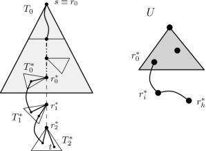
Figure 2: An example of path $Q$ contained in $H-F$ (left) and of the corresponding edges of $U$ (right). The length of $Q$ is upper-bounded by that of $P$.

The path $Q$ is composed of three parts, i.e. $Q=Q_{1}\circ Q_{2}\circ Q_{3}$. The first one, $Q_{1}$, coincides with $\pi_{T}(r^{*}_{0})$. The second one is obtained by considering the shortest path $\pi_{U}(r^{*}_{0},r_{h})$ and by replacing each edge going from a vertex $r^{*}_{i}\in V(U)$ to a vertex $r^{*}_{j}\in V(U)$ with the path: $\pi_{T}(r^{*}_{i},x^{\prime})\circ(x^{\prime},y^{\prime})\circ\pi_{T}(x^{\prime},r^{*}_{j})$, where $(x^{\prime},y^{\prime})$ is the edge associated to $(r^{*}_{i},r^{*}_{j})$ by Algorithm 1 when $v$ is considered. Finally, $Q_{3}=\pi_{T}(r^{*}_{h},t)$. In Figure 2, we show an example of how such path $Q$ can be obtained. We now prove that:

Lemma 4

$d_{H-F}(r,t)\leq w(Q)\leq w(P)$

Proof

Notice that the path $Q$ is in $H$ and does not contain any failed edge, hence $d_{H-F}(r,t)\leq w(Q)$ is trivially true.

To prove $w(Q)\leq w(P)$, notice that $P$ can also be decomposed into the three subpaths $P_{1}=P[r,r^{\prime}_{0}]$, $P_{2}=P[r^{\prime}_{0},r_{h}]$ and $P_{3}=P[r_{h},t]$. We have that that $P_{3}=Q_{3}$ and that the endpoints of $P_{2}$ coincide with the endpoints of $Q_{2}$. By the choice of $r^{*}_{0}$, we must have $w(Q_{1})+w(Q_{2})\leq w(P_{1})+w(P_{2})$ as the (weighted length of) path $P_{1}\circ P_{2}$ is considered in equation (1) when $z=r^{\prime}_{0}$. This implies that $w(Q)=w(Q_{1})+w(Q_{2})+w(Q_{3})\leq w(P_{1})+w(P_{2})+w(P_{3})=w(P)$.

By combining Lemma 2 with Lemma 3 and 4, it immediately follows:

Theorem 3.1

Algorithm 1 computes, in $O(n(m+f^{2}))$ time, a $(2|F|+1)$-PASPT of size $O(nf^{2})$, for any $|F|\leq f$.

We now relax the assumption that $U=U^{\prime}$. Indeed, if $k\neq 1$, Algorithm 1 computes, in line 1, a $(2k-1)$–spanner $U^{\prime}$ of the graph $U$. In this case, we can construct a path $Q^{\prime}$ in a similar way as we did for $Q$, with the exception that we now use the graph $U^{\prime}$ instead of $U$. Once we do so, it is easy to prove that a more general version of Lemma 4 holds:

Lemma 5

$d_{H-F}(r,t)\leq(2k-1)w(Q^{\prime})\leq(2k-1)w(P)$

Lemma 5, combined with Lemma 3, immediately implies that $d_{H-F}(r,t)\leq(2k-1)(2|F|+1)d_{G-F}(r,t)$. This discussion allows us to show an interesting trade-off between the size of the returned structure and the multiplicative stretch provided, as summarized by the following theorem:

Theorem 3.2

Let $k\geq 1$ be an integer. Then, Algorithm 1 can compute, in $O(n(m+f^{2}))$ time, a $(2k-1)(2|F|+1)$-PASPT of size $O(nk\cdot f^{1+\frac{1}{k}})$.

3.1 Oracle Setting

In what follows, we show how Algorithm 1 can be used to compute an approximate distance oracle of size $O(nf^{2})$ (see Algorithm 2). We also show that a smaller-size oracle can be obtained (see Algorithm 3) if we allow for a slightly larger query time.

1

2Preprocess $T=T_{G}(r)$ to answer LCA queries as shown in [16]

3 For each vertex $v\in V(G)$, compute and store its level $\ell(v)$.

4foreach $v\in V(G)$ do

5       Let $\langle r=z_{0},z_{1},\dots,z_{\ell}(v)$ be the path from $r$ to $v$ in $T$

6       Build graph $U$ associated with vertex $v$ as in Algorithm 1

7       Compute and store the solution to the all-pairs shortest paths problem on $U$

8       foreach $\eta=1,\dots,\min\{f,\ell(v)\}$ do

9             foreach  $r_{h}:h>\ell(v)-\eta$  do

10                   $R\leftarrow\{z_{i}:0\leq i\leq\ell(v)-\eta\}$

11                   Let $r^{*}_{0}$ be the vertex of $R$ minimizing Equation (1)

12                   Store $r^{*}_{0}$ with key $(v,\eta,r_{i})$

13                  

Algorithm 2 Algorithm for building an oracle with constant query time.

1

2Preprocess $T$ to answer LCA queries as shown in [16]

3 For each vertex $v\in V(G)$, compute and store its level $\ell(v)$.

4foreach $v\in V(G)$ do

5       Build graph $U$ associated with vertex $v$ as in Algorithm 1

6       Build and store a distance sensitivity oracle of $U$ with stretch $2k-1$

7      

Algorithm 3 Algorithm for building an oracle with $O(f)$ query time.

Theorem 3.3

Let $F$ be a path failure of $|F|\leq f$ edges and $t\in V(G)$. Algorithm 2 builds, in $O(n(m+f^{2}))$ time, an oracle of size $O(nf^{2})$ which is able to return:

• a $(2|F|+1)$-approximate distance in $G-F$ between $r$ and $t$ in constant time;

• the associated path in a time proportional to the number of its edges.

Proof

In order to answer a query we need to find: (i) the root $r^{*}_{0}$ of the subtree of $\mathcal{C}^{*}$ which contains $t_{0}$, (ii) the root $r_{h}$ of the subtree of $\mathcal{C}^{*}$ containing $t$. In order to find $r_{h}$, we perform a LCA query on $T$ to find the least common ancestor $u$ between $v$ and $t$. Either $\ell(v)\geq\ell(u)>\ell(v)-|F|$, in which case $u=r_{h}$, or $\ell(u)\leq\ell(v)-|F|$ which means that $t$ belongs to $T_{0}$. As in the latter case we can simply return $d_{T}(t)$, we focus on the former one. To find $r^{*}_{0}$ we look for the vertex associated with the triple $(v,|F|,r_{h})$ stored by Algorithm 2 at line 2.

We answer a distance query with the quantity $d_{T}(r^{*}_{0})+d_{U^{\prime}}(r^{*}_{0},r^{*}_{h})+d_{T}(r_{h},t)$, which can be computed in constant time by accessing the distances stored in shortest path tree $T$, plus the solution of the APSP problem on $U^{\prime}$ computed by Algorithm 2 when vertex $v$ was considered.

To answer a path query we simply construct, and return, the path $Q$, by expanding the edges of the graph $U^{\prime}$ into paths which are in $G-F$, as explained before. This clearly takes a time proportional to the number of edges of $Q$.

If we allow for a query time that is proportional to $O(f+k)$, we can reduce the size of the oracle by computing a distance sensitivity oracle (DSO) of $U$ (see Algorithm 3). In this case, we can still find vertex $r_{h}$ using the LCA query, as shown in the proof of Theorem 3.3, while vertex $r^{*}_{0}$ is guessed among the (up to) $f$ roots of the trees in $G-F^{*}$ which are contained in $T_{0}$. The resulting oracle is summarized by the following:

Theorem 3.4

Let $F$ be a path failure of $|F|\leq f$ edges, let $t\in V(G)$ and let $k\geq 1$ be an integer. Algorithm 3 builds, in $O(n(m+f^{2}))$ time, an oracle of size $O(nkf^{1+\frac{1}{k}})$ which is able to return:

• a $(2k-1)(2|F|+1)$-approximate distance in $G-F$ between $r$ and $t$ in $O(f+k)$ time;

• the corresponding path in $O(\ell+k+f)$ time, where $\ell$ is the number of its edges.

4 Our $3$-PASPT Structure for Paths of 2 Edges

In what follows, we provide an algorithm which builds a $3$-PASPT (see Algorithm 4) for the special case of at most $f=2$ cascading edge failures. This structure improves, w.r.t. the quality of the stretch, over the general $(2|F|+1)$-PASPT of Section 3.

Input : A graph $G$, $r\in V(G)$, an SPT $T=T_{G}(r)$

Output : A $3$-PASPT of $G$ rooted at $r$

1 $H\leftarrow T_{G}(r)$

2 $\hat{T}\leftarrow$ compute a $3$-EASPT of $T_{G}(r)$ as shown in [20]

3 $H\leftarrow E(H)\cup E(\hat{T})$

4 Compute a path decomposition $\mathcal{P}$ of $T_{G}(r)$ by recursively applying Lemma 6

5 foreach Path $P\in\mathcal{P}$ do

6       foreach $x\in V(P)\,:x$ is not a leaf and $x\neq r$ do

7             Let $z$ be the (unique) child of $x$ in $P$

8             Let $\hat{e}$ be the edge connecting $x$ and its parent int $T$

9            

            // Protect vertex $x$

10             $E(H)\leftarrow E(H)\cup\texttt{FirstLast}(\pi_{G-\hat{e}}(x),T_{G}(r,z))$

11             if $\pi_{G-\hat{e}}(x)$ contains an edge $e^{\prime}$ in $C(x)$ then

12                   $E(H)\leftarrow E(H)\cup\texttt{FirstLast}(\pi_{G-\hat{e}-e^{\prime}}(x),T_{G}(r,z))$

13                  

            // Protect vertex $z$

14             $E(H)\leftarrow E(H)\cup E(\pi_{G-\hat{e}}(z))$

15             foreach $e^{\prime}\in\{\pi_{G-\hat{e}}(z)\cap C(x)\}$ do

16                   $E(H)\leftarrow E(H)\cup E(\pi_{G-\hat{e}-e^{\prime}}(z))$

17                  

            // Protect all the other children of $x$

18             foreach children $z_{i}$ of $x\,\>\,z_{i}\neq z$  do

19                   Let $(u,q)$ be the first edge of $\pi_{G-\hat{e}-(x,z_{i})}(x,z_{i})$ with $q\in V(T_{G}(r,z_{i}))$

20                   $E(H)\leftarrow E(H)\cup\{(u,q)\}$

21                  

            // Protect vertices whose paths that do not contain $x$

22             $T^{\prime}\leftarrow T_{G-x}(r,$) with edges oriented towards the leaves

23             $E(H)\leftarrow E(H)\cup\{(x_{1},x_{2})\in E(T^{\prime})\,:\,x_{2}\not\in T_{G}(r,z)\}$

24            

return $H$

Algorithm 4 Algorithm for building a $3$-PASPT for the case of $f=2$.

The algorithm starts with a 3-EASPT with $O(n)$ edges [20] and proceeds as follows. As initial building block, it considers a suitable path $P$ in the shortest-path tree $T_{G}(r)$, and constructs a structure $H$ that is able to handle the failure of a pair of edges $\{e_{1},e_{2}\}$, such that $e_{1}\in P$, and guarantees $3$-stretched distances from $r$, for each vertex in $G$. Then, we make use of the following result of [2]:

Lemma 6 ([2])

There exists an $O(n)$ time algorithm to compute an ancestor-leaf path $Q$ in $T_{G}(r)$ whose removal splits $T_{G}(r)$ into a set of disjoint subtrees $T_{G}(r,r_{1}),\dots,T_{G}(r,r_{j})$ such that, for each $i\leq j$:

• $|T_{G}(r,r_{i})|<n/2$ and $V(Q)\cap V(T_{G}(r,r_{i}))=\emptyset$

• $T_{G}(r,r_{i})$ is connected to $Q$ through some edge for each $i\leq j$

This allows us to incrementally add edges to $H$ by considering a set $\mathcal{P}$ of edge-disjoint paths. This set can be obtained by recursively using the path decomposition technique of Lemma 6 on the shortest-path tree $T_{G}(r)$. We show that, in this way, we are able to build a $3$-PASPT of size $O(n\log n)$. Given a path $\pi=\langle s,\dots,t\rangle$ and a tree $T^{\prime}$, we denote by $\texttt{FirstLast}(\pi,T^{\prime})$ the edges of the subpaths of $\pi$ going (i) from $s$ to the first vertex of $\pi$ in $V(T^{\prime})$, and (ii) from the last vertex of $\pi$ in $V(T^{\prime})$ to $t$. If these vertices do not exists, i.e., $V(\pi)\cap V(T^{\prime})=\emptyset$, then we define $\texttt{FirstLast}(\pi,T^{\prime})=E(\pi)$. Moreover, we denote by $C(x)$ the edges connecting vertex $x$ to its children in $T_{G}(r)$. We are able to prove the following theorem, whose proof is given in the appendix:

Theorem 4.1

Let $F$ be a path failure of $|F|\leq 2$ edges and $t\in V(G)$. Algorithm 4 computes, in $O(nm+n^{2}\log n)$ time, a $3$-PASPT of size $O(n\log n)$.

Notice that it is possible to modify Algorithm 4 in order to build an oracle of size $O(n\log n)$ which is able to report, with optimal query time, both a $3$-stretched shortest path in $G-F$ and its distance, when $F$ contains two consecutive edges in $T$. Both the description of the modified algorithm and the proof of the following theorem is given in the appendix.

Theorem 4.2

Let $F$ be a path failure of $|F|\leq 2$ edges and $t\in V(G)$. A modification of Algorithm 4 builds, in $O(nm+n^{2}\log n)$ time, an oracle of size $O(n\log n)$ which is able to return:

• a $3$-approximate distance in $G-F$ between $r$ and $t$ in constant time;

• the associated path in a time proportional to the number its edges.

5 Experimental Study

In this section, we present an experimental study to assess the performance, w.r.t. both the quality of the stretch and the size (in terms of edges), of the proposed structures within SageMath (v. 6.6) under GNU/Linux.

As input to our algorithms, we used weighted undirected graphs belonging to the following graph categories: (i) Uncorrelated Random Graphs (ERD): generated by the general Erdős-Rényi algorithm [7]; (ii) Power-law Random Graphs (BAR): generated by the Barabási-Albert algorithm [1]; Quandrangular Grid Graphs (GRI): graphs whose topology is induced by a two-dimensional grid formed by squares. For each of the above synthetic graph categories we generated three input graphs of different size and density. We assigned weights to the edges at random, with uniform probability, within $[100,100\,000]$. We also considered two real-world graphs. In details: (i) a graph (CAI) obtained by parsing the CAIDA IPv4 topology dataset [17], which describes a subset of the Internet topology at router level (weights are given by round trip times); (ii) the road graph of Rome (ROM) taken from the 9th Dimacs Challenge Dataset (weights are given by travel times).

Then, for each input graph, we built both the $(2k-1)(2|F|+1)$-PASPT, for which we focused on the basic case of $k=1$, and the $3$-PASPT, as follows: we randomly chose a root vertex, computed the SPT and enriched it by using the corresponding procedures (i.e. Algorithm 1 and 4, resp.). We measured the total number of edges of the resulting structures.

Regarding Algorithm 1, we set $f=10$, as such a value has already been considered in previous works focused on the effect of path-like disruptions on shortest paths [5, 12]. Then, we randomly select path failures of $|F|$ edges to perform on the input graphs, with $|F|$ uniformly chosen at random within the range $[2,f]$. We removed the edges belonging to the path failure from both the original graph and the computed structure. Regarding Algorithm 4, we simply chose at random a pair of edges and removed them from both the original graph and the computed structure.

After the removal, we computed distances, from the root vertex, in both the original graph and the fault tolerant structure, and measured the resulting average stretch. In order to be fair, we considered only those nodes that get disconnected as a consequence of the failures. Our results are summarized in Table 1, where, for each input graph, we report the number of vertices and edges, the average size (number of edges) of the two fault tolerant structures and the corresponding provided average stretch.

G	|V(G)|	|E(G)|	$(2|F|+1)$-PASPT		$3$-PASPT
			#edges	avg stretch	#edges	avg stretch
ERD-1	500	50 000	3 980	1.8015	957	1.0000
ERD-2	1 000	50 000	8 899	1.1360	1 924	1.0000
ERD-3	5 000	50 000	20 198	1.0903	9 501	1.0035
BAR-1	500	1 491	1 366	1.0003	949	1.0041
BAR-2	1 000	2 991	2 765	1.0034	1 871	1.0005
BAR-3	5 000	14 991	13 349	1.0040	9 459	1.0000
GRI-1	500	1 012	1 008	1.0005	868	1.0000
GRI-2	1 000	1 984	1 973	1.0000	1 749	1.0000
GRI-3	5 000	9 940	9 884	1.0000	8 826	1.0000
CAI	5 000	6 328	6 033	1.0000	6 026	1.0000
ROM	3 353	4 831	4 796	1.0000	4 780	1.0000

Table 1: Average number of edges and stretch factor for both the $(2|F|+1)$-PASPT and the $3$-PASPT.

First of all, our results show that the quality of the stretch, provided by both the $(2|F|+1)$-PASPT and the $3$-PASPT in practice, is always by far better than the estimation given by the worst-case bound (i.e. 2|F|+1 and 3, resp.). In details, the average stretch is always very close to $1$ and does not depend neither on the input size nor on the number of failures. This is probably due to the fact that those cases considered in the worst-case analysis are quite rare.

Similar considerations can be done w.r.t. the number of edges that are added to the SPT by Algorithms 1 and 4. In fact, also in this case, the structures behave better than what the worst-case bound suggests. For instance, the number of edges of the $(2|F|+1)$-PASPT (the $3$-PASPT, resp.) is much smaller than $nf^{2}$ ($n\log n$, resp.). In summary, our experiments suggest that the proposed fault tolerant structures might be suitable to be used in practice.

Appendix 0.A Omitted Proofs

In this section, we upper-bound the running time of Algorithm 4. In details, we prove that, given a set of two failures $F=\{e_{1},e_{2}\}$, $d_{H-F}(t)\leq 3\cdot d_{G-F}(t)$ for every $t\in V(G)$, and that $H$ contains $O(n\cdot\log n)$ edges. W.l.o.g. we assume that that $e_{1}=(y,x)$, $e_{2}=(x,k)$, where $x$ is a child of $y$ and $k$ is a child of $x$ in $T$.

Notice that, every possible edge $e_{1}$ of a pair of failures that can occur on $T_{G}(r)$ is considered exactly once as, during the construction phase, we make use of the path decomposition technique of [2]. Let $P\in\mathcal{P}$ be the path of the path decomposition $\mathcal{P}$ which contains $e_{1}$ and let $z$ be the vertex following $x$ in $P$. Notice that the other failed edge $e_{2}=(x,k)$ might or might not belong to the very same path $P$.

We now bound the distance $d_{H-F}(t)$ between $r$ and a generic target vertex $t\in V(G)$. We assume, w.l.o.g., that $t$ belongs to $T_{G}(r,x)$ as otherwise we trivially have $d_{H-F}(t)=d_{G-F}(t)$. For the sake of clarity, we divide the proof into parts, depending on the position of $t$ in $T_{G}(r)-F$ and on the structure of the path $\pi_{G-F}(t)$.

Lemma 7

For every $t\in V(T_{G}(r,z))$, there exists a path $\pi^{*}(t)$ between $r$ and $t$ in $H-F$ such that $w(\pi^{*}(t))\leq 3\cdot d_{G-F}(t)$.

Proof

The edges added to $H$ at Lines 4–4 of Algorithm 4 guarantee that $d_{H-F}(z)$ equals $d_{G-F}(z)$ for every possible pair of failures. It follows that we can choose $\pi^{*}(t)=\pi_{G-F}(z)\circ\pi_{G}(z,t)$, as we have:

$$w(\pi^{*}(t)) =d_{H-F}(z)+d_{H-F}(z,t)$$

$$\leq d_{H-F}(z)+d_{G}(z,t) \pi_{G}(z,t)=\pi_{H-F}(z,t)$$ ()

$$\leq d_{G-F}(z)+d_{G}(z,t)$$ (By Lines 4–4 of Alg. 4)

$$\leq d_{G-F}(t)+d_{G-F}(t,z)+d_{G}(z,t)$$ (By triang. ineq.)

$$\leq d_{G-F}(t)+2d_{G}(t,z) \pi_{G}(z,t)=\pi_{G-F}(z,t)$$ ()

$$\leq d_{G-F}(t)+2d_{G}(t)\leq 3d_{G-F}(t). z\in V(\pi_{G})(t)$$ ()

Lemma 8

There exists a path $\pi^{*}(x)$ between $r$ and $x$ in $H-F$ such that $w(\pi^{*}(x))\leq 3\cdot d_{G-F}(x)$ if $e_{2}=(x,z)$ and $w(\pi^{*}(x))=d_{G-F}(x)$ otherwise.

Proof

If $V(\pi_{G-F}(x))\cap V(T_{G}(r,z))=\emptyset$ we set $\pi^{*}(x)=\pi_{G-F}(x)$ and we are done as $\pi^{*}(x)$ gets added to $H$ by Lines 4–4 of Algorithm 4.

Otherwise, if $V(\pi_{G-e_{1}-e_{2}}(x))\cap V(T_{G}(r,z))\neq\emptyset$, let $q,q^{\prime}$ be the first and last vertex of $\pi=\pi_{G-e_{1}-e_{2}}(x)$ that is in $V(T_{G}(r,z))$, respectively. If $e_{2}\neq(x,y)$ then it suffices to choose $\pi^{*}(x)=\pi$. Indeed, by construction, $\pi$ is in $H$ since both $\pi[r,q]$ and $\pi[q,x]=\pi_{G}(q,z)$ are in $H$.

Finally, if $e_{2}=(x,y)$, then $pi^{*}(x)=\pi^{*}(q^{\prime})\circ\pi[q^{\prime},x]$, where $\pi^{*}(q^{\prime})$ is the path of Lemma 7. The path $\pi^{*}(x)$ is in $H$ and we can bound its length as follows:

$$w(\pi^{*}(x))=w(\pi^{*}(q^{\prime}))+d_{G-F}(q^{\prime},x)\leq 3d_{G-F}(q^{\prime})+d_{G-F}(q^{\prime},x)\leq 3d_{G-F}(x).$$

Lemma 9

For every $t\not\in V(T_{G}(r,z))\cup\{x\}$ such that $x\not\in V(\pi_{G-F}(t))$, there exists a path $\pi^{*}(t)$ between $r$ and $t$ in $H-F$ satisfying $w(\pi^{*}(t))\leq 3\cdot d_{G-F}(t)$.

Proof

First of all notice that it must hold $\pi_{G-F}(t)=\pi_{G-x}(t)$. If $\pi_{G-x}(t)$ does not contain any vertex of $T_{G}(r,z)$ we are done, as we can set $\pi^{*}(t)=\pi_{G-x}(t)$ (by Lines 4–4 of Algorithm 4). Otherwise, let us call $q$ the last vertex of $\pi_{G-x}(t)$ that belongs to $T_{G}(r,z)$. We set $\pi^{*}(t)=\pi^{*}(q)\circ\pi_{G-x}(q,t)$, where $\pi^{*}(q)$ is the path of Lemma 7. We have

$$w(\pi^{*}(t)) =w(\pi^{*}(q))+d_{H-x}(q,t)$$

$$\leq 3d_{G-F}(q)+d_{H-F}(q,t)$$ (By Lemma 7)

$$\leq 3d_{G-F}(q)+d_{H-F}(q,t)$$ (By Lines 4–4 of Alg. 4)

$$\leq 3d_{G-F}(q)+3d_{G-F}(q,t)=3d_{G-F}(t) q\in V(\pi_{G-F}(t))$$ (Since )

Lemma 10

For every $t\not\in V(T_{G}(r,z))\cup\{x\}$ such that $x\in V(\pi_{G-F}(t))$, there exists a path $\pi^{*}(t)$ between $r$ and $t$ in $H-F$ satisfying $w(\pi^{*}(t))\leq 3\cdot d_{G-F}(t)$.

Proof

Notice that $t$ belongs to a subtree $T_{G}(r,z_{i})$ for exactly one child $z_{i}\neq z$ of $x$ in $T_{G}(r)$. If $(x,z_{i})\neq e_{2}$, we have that $\pi_{G}(x,t)=\pi_{G-F}(x,t)=\pi_{H-F}(x,t)$ We set $\pi^{*}(t)=\pi^{*}(x)\circ\pi_{G}(x,t)$ where $\pi^{*}(x)$ is the path of Lemma 8. We have:

$$w(\pi^{*}(t))=w(\pi^{*}(x))+d_{G}(x,t)\leq 3d_{G-F}(x)+d_{G-F}(x,t)\leq 3d_{G-F}(t)$$

Otherwise, $e_{2}=(x,z_{i})$, which means that $t$ belongs to a subtree of $T_{G}(r)$ which gets disconnected form $x$ by the removal of $e_{2}$.

Since $e_{2}\neq(x,z)$, we know that the path $\pi^{*}(x)$ of Lemma 8 satisfies $w(\pi^{*}(x))=d_{G-F}(x)$. Moreover, the shortest path $\pi_{G-F}(x,z_{i})$ traverses at most one other subtree (other than $T_{G}(r,z_{i})$) rooted at a child of $x$. This is because $H-F$ contains the shortest paths from $x$ to every vertex in $V(T_{G}(r,x))\setminus V(T_{G}(r,z_{i}))$. Let $(u,q)$ be the first edge of the path $\pi_{G-F}(x,z_{i})$ such that $q\in V(T_{G}(r,z_{i}))$ and notice that this edge belongs to $H$ (Lines 4–4 of Algorithm 4). By the choice of $(u,q)$ we have $\pi_{H-F}(x,q)=\pi_{G}(x,u)\circ(u,q)$. We set $\pi^{*}(t)=\pi^{*}(x)\circ\pi_{G}(x,u)\circ(u,q)\circ\pi_{G}(q,z_{i})\circ\pi_{G}(z_{i},t)$.

$$w(\pi^{*}(t)) =w(\pi^{*}(x))+d_{G}(x,u)+w(u,q)+d_{G}(q,z_{i})+d_{G}(z_{i},t)$$

$$\leq d_{G-F}(x)+d_{G-F}(x,q)+d_{G-F}(q,z_{i})+d_{G}(z_{i},t)$$

$$\leq d_{G-F}(x)+d_{G-F}(x,z_{i})+d_{G}(z_{i},t) q\in V(\pi_{G-F}(x,z_{i}))$$ (Since )

$$\leq d_{G-F}(x)+d_{G-F}(x,t)+2d_{G}(z_{i},t)$$ (By triang. ineq.)

$$\leq d_{G-F}(x)+d_{G-F}(x,t)+2d_{G}(x,t) z_{i}\in V(\pi_{G})(x,t)$$ ()

$$\leq d_{G-F}(x)+d_{G-F}(x,t)+2d_{G-F}(x,t)$$

$$=d_{G-F}(x)+3d_{G-F}(x,t)\leq 3d_{G-F}(t). x\in V(\pi_{G-F}(t))$$ (Since )

We now bound the size of $H$. In order to do so, it is useful to split the vertices of the $T$ into components, depending on the vertex $x$ that is currently considered by Algorithm 4. More formally, when a couple of edges $(y,x),(x,z)$ is considered we can partition the vertices of $T-x$ into three distinct sets (see Figure 3):

• $U_{x}$, which contains the vertices which are in the same subtree as $r$ in $T-x$;

• $D_{x}$, which contains the vertices which are in the subtree of $T$ rooted at $z$:

• $O_{x}$, which contains all the vertices which are in the subtree rooted at some child $z_{i}\neq z$ of $x$ in $T$.

We are now read to prove:

Lemma 11

The structure $H$ returned by Algorithm 4 contains $O(n\cdot\log n)$ edges.

Proof

To prove the claim we fix a generic path $P=\langle u,\dots,v\rangle$ (of at least two edges) of the path decomposition, where $v$ is a left and $u$ one its ancestors in $T$. We show that, when Algorithm 4 considers $P$, the total number of edges added to $H$ is $O(|V(T_{G}(r,u))|)$.

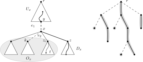
Figure 3: Left: a view of the partition of the vertices induced by the removal of a pair of edges of $E(T_{G}(r))$. Right: A path decompostion of a tree. Paths of the decomposition are highlighted. Edges connecting the roots of the resulting subtrees to a path of the decomposition are dashed.

For the sake of the analysis, imagine the edges of paths considered by the algorithm as if they were directed. Notice that no new edge entering a vertex in $U_{x}$ can be added to $H$, as the shortest paths towards vertices in $U_{x}$ cannot change, and $H$ contains a shortest path tree $T$ of $G$. Hence, in the following, we ignore all the edges entering vertices in $U_{x}$.

In Lines 4–4, the edges of at most two paths are added to $H$. Moreover, by definition of $\texttt{FirstLast}(\cdot,\cdot)$, at most one edge of each path enters a vertex in $D_{x}$. This implies that the number of new edges is at most $O(O_{x})$. In Lines 4–4, at most $3$ paths are considered as $\{\pi_{G-e_{1}}(z)\cap C(x)\}$ contains at most $2$ edges. Each of those paths has at most one new edge which enters a vertex $q$ in $D_{z}$ since, once this happens, the shortest path from $q$ to $z$ of $T$ is already in $H$. Again, the number of new edges is at most $O(O_{x})$. In Lines 4–4, at most one edge for each children of $z_{i}\neq z$ of $x$ is added to $H$, and all those children belong to $O_{x}$. Finally, in Lines 4–4 only new edges entering vertices in $O_{x}$ are added to $H$, so their overall number is $O(O_{x})$.

As all the sets $O_{x}$ associated to the different vertices $x$ of $P$ are pairwise vertex disjoint, we immediately have that at most $O(|V(T_{G}(r,v))|)$ edges are added to $H$ when path $P$ is examined.

The first path $P$ considered by Algorithm 4 is the one obtained by applying Lemma 6 on $T$. The removal of this path splits $T$ into a number $h$ of subtrees $T_{1},\dots,T_{h}$ having $\eta_{1},\dots,\eta_{h}$ vertices respectively. Moreover we know that $\eta_{i}\leq\frac{n}{2}\;\forall i=1,\dots,h$ and that $\sum_{i=1}^{h}\eta_{i}\leq n$. If we reapply the procedure recursively, we get the following recurrence equation describing the overall number of new edges:

$$S(n)=\sum_{i=1}^{h}S(\eta_{i})+n$$

which can be solved to show that $S(n)=O(n\log n)$. To conclude the proof, we only need to notice that the set of paths $\mathcal{P}$ used by Algorithm 4 is defined exactly in this very same recursive fashion, and that the tree $\hat{T}$ has $O(n)$ edges.

Finally, we bound the running time of Algorithm 4:

Lemma 12

Algorithm 4 requires $O(nm+n^{2}\log n)$ time.

Proof

First of all, observe that a rough estimate of the time needed for computing the path decomposition $\mathcal{P}$ is $O(n^{2})$ and that the time needed to build $\hat{T}$ is $O(nm)$ [20]. Moreover each vertex $x$ get considered at most once.

When the algorithm is considering a vertex $x$, a constant number of different shortest paths are needed. Those can be computed in $O(m+n\log n)$ time using the Dijkstra’s algorithm where, for each vertex $v$, we also store the last edge of its shortest path that (i) leaves the same connected component of $r$ in $T-F$, (ii) leaves $T_{G}(r,z)$, and (iii) enters the same connected component as $v$ in $T-F$. This allows to implement $\texttt{FirstLast}(\cdot)$ and to add the edges needed in Lines 4–4, 4–4 in time proportional to the vertices in $O_{x}$. Hence, the overall time spent by adding edges to $H$ is again $O(n\log n)$.

By Lemmata 7–11, Theorem 4.1 follows.

Appendix 0.B Oracle Setting for $f=2$ and Proof of Theorem 4.2

We here give a brief description of how to modify Algorithm 4 in order to build an oracle of size $O(n\cdot\log n)$ which is able to report, with optimal query time, both a $3$-stretched shortest path in $G-F$ and its distance, when $F$ contains two consecutive edges in $T$.

In order to do so, we first add an additional step to Algorithm 4 which computes an $O(n)$ size structure which is able to answer LCA queries in $O(1)$ time [16]. Then we store the tree $T$ and, for each vertex $x$, its child $z$ on the path decomposition.

Whenever we are considering a vertex $x$ and its child $z\in P$, we also store each path, say $\pi$, towards a vertex, say $u$, considered in Lines 4–4, 4–4, using a compact representation. To be more precise, let $s$ be the last vertex of $\pi$ which belongs to the same component as $r$ in $T-F$, and let $q,q^{\prime}$ be the first and last vertex of $\pi$ which belong to $T(z)$. We only store the (i) vertices $s,q,q^{\prime}$, (ii) the subpaths $\pi[s:q]$, $\pi[q^{\prime},u]$ along with their lengths, and (iii) a reference to the position $x$ in the subpaths of $\pi$, if any. If $q,q^{\prime}$ do not exists, we simply store $s$, $\pi[s:u]$, $w(\pi[s,u])$, and a reference to $x$.

In Lines 4–4, we add one edge $(u,q)$ for each children $z_{i}\neq z$ of $x$. We store $(u,q)$ alongside $z_{i}$.

Finally, in Lines 4–4, we add some edges of the shortest path tree $T_{G-x}(r)$. For each vertex $u\in O_{x}$, we store (i) the edge leading to its parent in $T_{G-x}(r)$, (ii) the last vertex $q$ of $pi_{G-x}(u)$ which is either in $U$ or in $V(T_{G}(r,z))$, (iii) the length of $\pi_{G-x}(u)[q,u]$, and iv) the root of the subtree containing $u$ in $T-x$.

Since the amount of memory used to do so is always proportional to the vertices in $O_{x}$ we have that the overall size is still $O(n\log n)$. It is easy to see that, given a path failure $F=\{(y,x),(x,k)\}$ and a vertex $t$, we can answer a query by building (or computing the distance of) $\pi^{*}(t)$ as described in the appropriate lemma in Lemmata 7–10. In order to do so we need to know:

• The root of the subtrees of $T-x$ containing $t$.

• Whether $\pi_{G-F}(t)$ contains $x$.

The former can be easily done by querying, in constant time, the least common ancestors of the pairs $t,z$ and $t,x$ in $T$ to determine if $z$ belongs to $U$ or $T_{G}(r,z)$. If that is not the case, then the root of the sought subtree was explicitly stored and can be retrieved. As for the latter, we consider both cases. That is, we compute two candidate paths, we discard the one containing $(x,z_{i})$, if any (this is done using the pointers to $x$), and we return the shortest of the remaining paths (or its distance). The above reasoning suffices to prove Theorem 4.2.

References

- [1] R. Albert and A.-L. Barabási. Emergence of scaling in random networks. Science, 286:509–512, 1999.
- [2] S. Baswana and N. Khanna. Approximate shortest paths avoiding a failed vertex: Near optimal data structures for undirected unweighted graphs. Algorithmica, 66(1):18–50, 2013.
- [3] S. Baswana and S. Sen. Approximate distance oracles for unweighted graphs in õ(n2) time. In Proc. of 15th ACM-SIAM Symposium on Discrete Algorithms (SODA), pages 271–280, 2004.
- [4] S. Baswana and S. Sen. Approximate distance oracles for unweighted graphs in expected O(n2) time. ACM Transactions on Algorithms, 2(4):557–577, 2006.
- [5] R. Bauer and D. Wagner. Batch dynamic single-source shortest-path algorithms: An experimental study. In Proc. of 8th International Symposium on Experimental Algorithms (SEA), volume 5526 of Lecture Notes in Computer Science, pages 51–62. Springer, 2009.
- [6] D. Bilò, L. Gualà, S. Leucci, and G. Proietti. Fault-tolerant approximate shortest-path trees. In Proc. of 22nd European Symposium on Algorithms (ESA), volume 8737 of Lecture Notes in Computer Science, pages 137–148. Springer, 2014.
- [7] B. Bollobás. Random Graphs. Cambridge University Press, 2001.
- [8] S. Chechik. Approximate distance oracles with constant query time. In Proc. of 46th ACM Symposium on Theory of Computing (STOC), pages 654–663, 2014.
- [9] S. Chechik, M. Langberg, D. Peleg, and L. Roditty. Fault-tolerant spanners for general graphs. In Proc. of 41st ACM Symposium on Theory of Computing (STOC), pages 435–444. ACM, 2009.
- [10] S. Chechik, M. Langberg, D. Peleg, and L. Roditty. f-sensitivity distance oracles and routing schemes. In Proc. of 18th European Symposium on Algorithms (ESA), volume 6346 of Lecture Notes in Computer Science, pages 84–96. Springer, 2010.
- [11] A. D’Andrea, M. D’Emidio, D. Frigioni, S. Leucci, and G. Proietti. Dynamically maintaining shortest path trees under batches of updates. In Proc. of 20th International Colloquium on Structural Information and Communication Complexity (SIROCCO), volume 8179 of Lecture Notes in Computer Science, pages 286–297. Springer, 2013.
- [12] A. D’Andrea, M. D’Emidio, D. Frigioni, S. Leucci, and G. Proietti. Experimental evaluation of dynamic shortest path tree algorithms on homogeneous batches. In Proc. of 13th International Symposium on Experimental Algorithms (SEA), volume 8504 of Lecture Notes in Computer Science, pages 283–294. Springer, 2014.
- [13] P. Erdős. Extremal problems in graph theory. In Theory of Graphs and its Applications, pages 29–36, 1964.
- [14] F. Grandoni and V.V. Williams. Improved distance sensitivity oracles via fast single-source replacement paths. In Proc. of 53rd IEEE Symposium on Foundations of Computer Science (FOCS), pages 748–757. IEEE, 2012.
- [15] L. Gualà and G. Proietti. Exact and approximate truthful mechanisms for the shortest paths tree problem. Algorithmica, 49(3):171–191, 2007.
- [16] D. Harel and R. E. Tarjan. Fast algorithms for finding nearest common ancestors. SIAM J. Comput., 13(2):338–355, 1984.
- [17] Y. Hyun, B. Huffaker, D. Andersen, E. Aben, C. Shannon, M. Luckie, and KC Claffy. The CAIDA IPv4 routed/24 topology dataset. http://www.caida.org/data/active/ipv4_routed_24_topology_dataset.xml.
- [18] H. Ito, K. Iwama, Y. Okabe, and T. Yoshihiro. Polynomial-time computable backup tables for shortest-path routing. In Proc. of 10th Internaltional Colloquium on Structural Information Complexity (SIROCCO), volume 17 of Proceedings in Informatics, pages 163–177. Carleton Scientific, 2003.
- [19] A. Mereu, D. Cherubini, A. Fanni, and A. Frangioni. Primary and backup paths optimal design for traffic engineering in hybrid igp/mpls networks. In Proc. of 7th International Workshop on Design of Reliable Communication Networks (DRCN), pages 273–280. IEEE, 2009.
- [20] E. Nardelli, G. Proietti, and P. Widmayer. Swapping a failing edge of a single source shortest paths tree is good and fast. Algorithmica, 35(1):56–74, 2003.
- [21] M. Parter and D. Peleg. Fault tolerant approximate BFS structures. In Proc. of 25th ACM-SIAM Symposium on Discrete Algorithms (SODA), pages 1073–1092. SIAM, 2014.
- [22] L Roditty, M. Thorup, and U. Zwick. Deterministic constructions of approximate distance oracles and spanners. In Proc. of 32nd International Colloquium, Automata, Languages and Programming (ICALP), volume 3580 of Lecture Notes in Computer Science, pages 261–272. Springer, 2005.
- [23] M. Thorup and U. Zwick. Approximate distance oracles. Journal of ACM, 52(1):1–24, 2005.