Nonlocal transport in a hybrid two-dimensional topological insulator

Abstract

We study nonlocal resistance in an H-shaped two-dimensional HgTe/CdTe quantum well consist of injector and detector, both of which can be tuned in the quantum spin Hall or metallic spin Hall regime. Because of strong spin-orbit interaction, there always exist spin Hall effect and the nonlocal resistance in HgTe/CdTe quantum well. We find that when both detector and injector are in the quantum spin Hall regime, the nonlocal resistance is quantized at $0.25\frac{h}{e^{2}}$, which is robust against weak disorder scattering and small magnetic field. While beyond this regime, the nonlocal resistance decreases rapidly and will be strongly suppressed by disorder and magnetic field. In the presence of strong magnetic field, the quantum spin Hall regime will be switched into the quantum Hall regime and the nonlocal resistance will disappear. The nonlocal signal and its various manifestation in different hybrid regimes originate from the special band structure of HgTe/CdTe quantum well, and can be considered as the fingerprint of the helical quantum spin Hall edge states in two-dimensional topological insulator.

I introduction

A topological insulator is a special quantum matterKane and Mele (2005a). Due to its particular band structure that the bulk states have a gap and the surface states can exist in the bulk band gap, the topological insulator behaves as an insulator in its interior and behaves as a metal on the surface. This leads to quantum spin Hall (QSH) effect. Different from magnetic field induced quantum Hall effect where the time-reversal symmetry is broken, the QSH effect arises from strong spin-orbit interaction (SOI) and is protected by the time-reversal symmetry. In the QSH regime, the electron spins are locked to their momenta and the boundary states are helical, i.e., there are two time reversed counter propagating edge states occupied by electrons with opposite spin. Such a topological state can be signed by $Z_{2}$ indexKane and Mele (2005b). In topological insulator, the boundary states are protected by the time-reversal symmetry and the backscattering between boundary states is strongly suppressed. As a result, the helical edge states are robust against the non-magnetic disorder.Jiang et al. (2009a) In the bulk energy band beyond the QSH phase, the topological insulator behaves as a metal, which is different from the conventional two-dimensional (2D) metal. In conventional metal, the electron wave functions are localized as long as there exists any weak disorderAbrahams (1979). However, in topological insulator, the metal state can exhibit quantum conductance in the moderate disorder, which is called topological Anderson insulator phenomenaLi et al. (2009); Xing et al. (2011); Jiang et al. (2009).

Up to now, the topological states have been predicted theoretically in several materials, such as the HgTe/CdTe quantum wellKonig et al. (2007); Bernevig et al. (2006), the InAs/GaSb quantum wellLiu et al. (2008a); Knez et al. (2011, 2012), the monolayer graphene with intrinsic SOIKane and Mele (2005b, a); Yao et al. (2007), and the gated bilayer grapheneMartin et al. (2008) that contains the one-dimensional chiral edge states. In experiment, the HgTe/CdTe quantum well and the InAs/GaSb quantum well with inverted band have been successfully discovered as 2D topological insulators with the QSH phaseBernevig et al. (2006). Since the discovery of the topological insulator, many works have been concentrated on the verification of its helical edge states. Such as, Konig and co-workersKonig et al. (2007) observed a quantized longitudinal conductance at about $2e^{2}/h$ that is consistent with the number of edge states predicted theoretically. Then, the transport along the edge states was confirmedRoth et al. (2009); Buttiker (2009). However, it remained to be shown that whether the transport due to the helical edge states is spin polarized. For this purpose, Br$\ddot{u}$ne and co-workersBrune et al. (2012) designed another experiment, in which the QSH effect and metallic spin Hall (MSH) effect are combined in a single HgTe/CdTe quantum well device using split gate technique. Through observation of nonlocal resistance in a H-shaped device, the spin polarization of edge state is then determined. In the work, in order to estimate the nonlocal resistance, the semiclassical simulation are performedBrune et al. (2012), but it breaks down when the chemical potential is close to the insulating gap. It is nowhere near enough for the QSH system. On the other hand, the nonlocal transport originates from the Hall effect, including the quantum Hall effect and the spin Hall effect. So, we must carefully examine the nonlocal effect to illustrate the role of the QSH state. Furthermore, as shown in the above experiments, the nonlocal signal deviated from the standard pattern predicted theoretically because of the various impurity and dephasing effect. Therefore, the detailed mechanism of the nonlocal transport in HgTe/CdTe quantum well, especially for the nonlocal transport in the QSH regime, is not very clear.

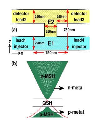
Figure 1: (Color online) (a) Sketch of the H-shaped hybrid four-terminal system. Through spilt gate technique, the on-site energies $E1$ and $E2$ in the injector (green region) and detector (yellow region) can be tuned separately. In the system, the scattering region (shadowed region) is connected to four leads. (b) Band structure of HgTe/CdTe: the conduction band (n-type carriers corresponding to n-MSH effect) and the valence band (p-type carriers corresponding to p-MSH effect) are separated by bulk band gap which holds the helical edge states and consequently the QSH effect.

In this paper, based on a four-band tight-binding model and aided by Keldysh nonequilibrium Green’s function, we study the nonlocal transport in a hybrid HgTe/CdTe quantum well, especially in the QSH regime. Following the recent experiment by Br$\ddot{u}$ne et. al.Brune et al. (2012), we consider an H-shaped device based on the HgTe/CdTe quantum well as shown in Fig.1(a). The on-site energies $E1$ and $E2$ in the bottom (green) and top (yellow) regions can be tuned separately by the split gates above the two regions. As a result, the two regions can then be in the QSH or MSH regime [see Fig.1(b)]. When changing $E1$ and $E2$, the quantum well will be in different regime, i.e., different hybrid structure, including QSH-QSH regime, QSH-MSH regime, and MSH-MSH regime. When injecting current from the bottom two terminals, spin accumulation or spin polarized potential is generated in the bridge between the bottom and top terminals due to the spin Hall effect. Then, because of the inverse SHE, the charge voltage will be detected in the top two terminals and leads to the nonlocal resistance in the HgTe/CdTe quantum well. It is obvious that there exists nonlocal resistance in all the hybrid devices because of the spin Hall effect. However, their manifestation is very different. For example, the nonlocal resistance in QSH-QSH device is quantized with the value of $\frac{h}{4e^{2}}$, that is robust against moderate disorder and weak magnetic field, while the nonlocal resistance in MSH-QSH or MSH-MSH device is oscillating and fragile. In the presence of strong magnetic field, the quantized nonlocal resistance will shrink and disappear finally. All these features of the nonlocal resistance: the robust quantized nonlocal resistance in the QSH regime, the fragile nonlocal resistance in the MSH regime, and the vanishing nonlocal resistance in the presence of strong magnetic field, are the particular characters of HgTe/CdTe quantum well, which can be derived from the special band structure of HgTe/CdTe quantum well. The details will be expatiated in the section III.

The rest of the paper is organized as follows. In Sec. II, based on the four-band tight-binding representation, the model Hamiltonian of system including central scattering region and attached leads is introduced. The formalisms for calculating the Green’s functions and nonlocal resistance are then derived. Sec. III gives numerical results together with detailed discussions. Finally, a brief summary is presented in Sec. IV.

II model and Hamiltonian

The whole system we consider is composed of the HgTe/CdTe quantum well with inverted band. In general, the structure of quantum well is asymmetry, which leads to the external Rashba SOI. The Hamiltonian of the system can be written as $H(k)=H_{0}(k)+H_{R}(k)$, where $H_{R}$ comes from the Rashba SOI, and

$$H_{0}(k)=\left(\begin{array}[]{cc}H_{\uparrow}(k)&0\\ 0&H_{\downarrow}(k)\end{array}\right).$$ (3)

From the time-reversal symmetry, we can get $H_{\uparrow}({\bf k})=H^{*}_{\downarrow}(-{\bf k})$, where

$$H_{\uparrow}({\bf k}) = \hbar v_{F}({\bf k}_{x}\sigma_{x}-{\bf k}_{y}\sigma_{y})+(m+C{\bf k}\cdot{\bf k})\sigma_{z}$$ (4)

$$+ D{\bf k}\cdot{\bf k}\sigma_{0},$$

where $\sigma_{x,y,z}$ are Pauli matrices presenting the pseudo spin formed by $s$ and $p$ orbitals, $\sigma_{0}$ is the $2\times 2$ unitary matrix in the pseudo spin space. $v_{F}$ is Fermi velocity. C, D, and m are the system parameters, which can be experimentally controlled. While the Hamiltonian due to Rashba SOI $H_{R}$ is expressed as

$$H_{R}(k)=\left(\begin{array}[]{cccc}0&0&it_{R}k_{-}&0\\ 0&0&0&0\\ -it_{R}k_{+}&0&0&0\\ 0&0&0&0\end{array}\right)$$ (9)

where $t_{R}$ is the Rashba SOI strength.

Equations (3) and (9) are the low-energy effective Hamiltonians of the HgTe/CdTe quantum wellBernevig et al. (2006); Liu et al. (2008) from the $k\cdot p$ perturbation. For an ideal crystal lattice, i.e., the infinite periodic system, the momentum $k$ is a good quantum number. In this case, using Hamiltonians (3) and (9) is convenient. However, here we consider charge transport in the H-shaped system, Hamiltonian can’t be expressed in momentum space, it should be expressed in real space. To do this, we substitute ${\bf k}$ with $-i\nabla$ and use the finite-difference approximation, then the total Hamiltonian $H$ is transformed into the tight-binding Hamiltonian in square lattice. It is given byLi et al. (2009); Jiang et al. (2009)

$$H = \sum_{\bf i}d^{\dagger}_{\bf i}H_{\bf ii}d_{\bf i}$$ (10)

$$+\sum_{\bf i}d_{\bf i}^{\dagger}H_{{\bf i},{\bf i}+{\bf a}_{x}}e^{i\phi_{{\bf i},{\bf i}+{\bf a}_{x}}}d_{{\bf i}+{\bf a}_{x}}+h.c.$$

$$+\sum_{\bf i}d_{\bf i}^{\dagger}H_{{\bf i},{\bf i}+{\bf a}_{y}}d_{{\bf i}+{\bf a}_{y}}+h.c.,$$

where $d_{\bf i}=[d_{s,{\bf i},\uparrow},d_{p,{\bf i},\uparrow},d_{s,{\bf i},\downarrow},d_{p,{\bf i},\downarrow}]^{T}$ with ‘$T$’ denoting transpose, and $d_{s(p),{\bf i},\uparrow(\downarrow)}$ and $d_{s(p),{\bf i},\uparrow(\downarrow)}^{\dagger}$ are the annihilation and creation operators for $s$ or $p$ orbital at site ${\bf i}$ with spin up or spin down, respectively. ${\bf i}=({\bf i}_{x},{\bf i}_{y})$ is the index of the discrete site of the system in the square lattice, and ${\bf a}_{x}=(a,0)$ and ${\bf a}_{y}=(0,a)$ are the unit vectors of the square lattice with $a$ the lattice constant. In zero magnetic field, the Hamiltonian (10) possesses time-reversal invariant. In the presence of a uniform perpendicular magnetic field ${\mathbf{B}}=[0,0,B]$, the time-reversal symmetry is broken. In coulomb gauge, considering the seimi-infinite leads being along the $x$-direction, the vector potential is set as ${\mathbf{A}}=[-By,0,0]$ which is $y$ dependent but periodic in the $x$-direction. In this case, a phase $\phi_{\bf ij}$ is generated in the hopping term $H_{{\bf i},{\bf i}+{\bf a}_{x}}$. The phase $\phi_{\bf ij}=\int_{\mathbf{i}}^{\mathbf{j}}{\mathbf{A}}\cdot d{\mathbf{l}}/\phi_{0}$ with flux quanta $\phi_{0}=\hbar/e$. In Eq.(10), $H_{\bf ii}$ and $H_{{\bf i},{\bf i}+{\bf a}_{x}({\bf a}_{y})}$ are all $4\times 4$ block matrix that are expressed as

$$H_{\bf ii}=(\epsilon_{\bf i}-\frac{4D}{a^{2}})(s_{0}\otimes\sigma_{0})+(m-4\frac{C}{a^{2}})(s_{0}\otimes\sigma_{z})$$

$$H_{{\bf i},{\bf i}+{\bf a}_{x}}=\frac{D}{a^{2}}(s_{0}\otimes\sigma_{0})+\frac{C}{a^{2}}(s_{0}\otimes\sigma_{z})$$

$$~{}~{}~{}~{}~{}~{}~{}~{}~{}-i\frac{\hbar v_{F}}{2a}(s_{z}\otimes\sigma_{x})+i\frac{t_{R}}{2a}(s_{y}\otimes\frac{\sigma_{0}+\sigma_{z}}{2})$$

$$H_{{\bf i},{\bf i}+{\bf a}_{y}}=\frac{D}{a^{2}}(s_{0}\otimes\sigma_{0})+\frac{C}{a^{2}}(s_{0}\otimes\sigma_{z})$$

$$~{}~{}~{}~{}~{}~{}~{}~{}~{}+i\frac{\hbar v_{F}}{2a}(s_{0}\otimes\sigma_{y})-i\frac{t_{R}}{2a}(s_{x}\otimes\frac{\sigma_{0}+\sigma_{z}}{2}),$$ (11)

where $s_{x,y,z}$ are the pauli matrices denoting the real spin and $s_{0}$ is the $2\times 2$ unitary matrix extented in real spin space. $\epsilon_{\bf i}=E1(E2)+w_{\bf i}$ with $E1$ and $E2$ being the on-site energies in detector (yellow) and injector (green) regions in Fig.1(a). $w_{\bf i}$ comes from the disorder effect that is a random on-site potential which is uniformly distributed in the region $[-w/2,w/2]$.

Based on above Hamiltonian, the charge current flowing to the $p$-th lead can be calculated from the zero temperature Landauer-Buttiker formulaDatta (Cambridge University Press, Cambridge, England, 1995)

$$J_{p}=\frac{e^{2}}{h}\sum_{q}T_{pq}(V_{p}-V_{q})$$ (12)

where $p,q=1,2,3,4$ are the index of the four leads. $T_{pq}$ is the transmission coefficient from terminal q to terminal p. In the following, we derive $T_{pq}$ in the system without and with Rashba SOI. In the absence of Rashba SOI, the Hamiltonian with spin up and spin down are decoupled, and the self energy and Green’s functions for the system with spin up and spin down can be calculated separately. Then transmission $T_{pq}=T_{pq,\uparrow}+T_{pq,\downarrow}$ and $T_{pq,\sigma}(E)=Tr_{r,o}[\Gamma_{p,\sigma}G^{r}_{pq,\sigma}\Gamma_{q,\sigma}G^{a}_{qp,\sigma}]$, where the ”${\rm Tr}_{r,o}$” denotes the trace over real space and orbital space (s and p orbitals), the line-width function $\Gamma_{q,\sigma}=i[\Sigma^{r}_{q,\sigma}-\Sigma^{r,\dagger}_{q,\sigma}]$, and $G^{r}_{pq,\sigma}$ is the Green’s function matrix whose rows and columns mark the lattices that are nearest to $p$ and $q$ lead respectively. The Green’s function $G^{r}_{\sigma}(E)=G^{a,\dagger}_{\sigma}(E)=(EI-H_{\sigma}-\sum_{q}\Sigma^{r}_{q,\sigma})^{-1}$, where $H_{\sigma}$ is Hamiltonian matrix with spin $\sigma$ in the central region and $I$ is the unit matrix with the same dimension as that of $H_{\sigma}$, and $\Sigma^{r}_{q,\sigma}$ is the retarded self-energy function contributed by the electrons with spin $\sigma$ in lead $q$. The self energy function can be obtained from $\Sigma^{r}_{p,\sigma}=H_{cp,\sigma}g^{r}_{p,\sigma}H_{pc,\sigma}$, where $H_{cp,\sigma}$ is the coupling from central region to lead $p$ and $g^{r}_{p,\sigma}$ is the surface retarded Green’s function of semi-infinite lead $p$ which can be calculated using transfer-matrix methodLee and Joannopoulos (1981a, b). When considering Rashba SOI, electrons spins (spin up and spin down) are coupled with each other and the total transmission $T_{pq}(E)=Tr_{r,o,s}[\Gamma_{p}G^{r}_{pq}\Gamma_{q}G^{a}_{qp}]$, where the ”${\rm Tr}_{r,o,s}$” is the trace over real space, orbital space and spin space.

In the following, we calculate the nonlocal response, i.e., the voltage response (detector) in top region on the current (injector) in bottom region, which can be denoted by nonlocal resistance $R_{23,14}$. We also calculator $R_{14,23}$, i.e., the voltage response in bottom region on the current in top region. $R_{23,14}$ and $R_{14,23}$ have the nearly same properties, so, we focus on $R_{23,14}$ in the following. We apply a bias V across the injector terminals 1 and 4 to inject current. For the detector terminals 2 and 3, the currents are set to zero. Then use the boundary conditions $V_{1}=V$, $V_{4}=0$, $J_{2}=J_{3}=0$, we can calculate the current $J_{1}=-J_{4}$ and the voltages $V_{2}$ and $V_{3}$ in the voltage probes from the Landauer-Buttiker formula. Finally, the nonlocal resistance is given by $R_{23,14}\equiv(V2-V3)/J_{1}$.

III numerical results and analysis

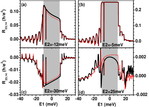
Figure 2: $R_{23,14}$ vs on-site energy $E1$ in the injector region with Rashba SOI $\alpha=0$ (black solid lines) and $50meVnm$ (red dotted lines). Panels (a), (b), (c), and (d) correspond to $E2=-12meV$, $-5meV$ $-30meV$ and $25meV$, respectively, where $E2$ is the on-site energy in the detector (top region). The gray region in panel (a,b,c,d) is the range of bulk energy gap of injector (the sample bottom).

In the numerical calculation, the parameters of the HgTe/CdTe quantum well are set as $\hbar v_{F}=364.5meVnm$, $C=-686meVnm^{2}$, $D=-512meVnm^{2}$, and the effective mass is taken as $m=-10meV$, which corresponds to the realistic quantum well with thickness $d=7nm$.Konig et al. (2008) It exceeds the critical thickness $d_{c}=6.3nm$ and induces the inverted band, which leads to the topological phase. Comparing to the inverted InAs/GaSb/AlSb quantum well, the Rashba SOI in HgTe/CdTe quantum well is very small and can be usually neglected in the numerical calculation. However, in order to quantitatively estimate the effect of Rashba SOI, we set a nonzero Rashba SOI. The strength of Rashba SOI is set to $\alpha=50meVnm$. It is a very large value, because the Rashba SOI in inverted InAs/GaSb/AlSb quantum well is only $\alpha=71meVnm$,Liu et al. (2008a) while Rashba SOI in HgTe/CdTe quantum well is much smaller than that in InAs/GaSb/AlSb quantum well. Furthermore, we set lattice constant $a=5nm$, that is small enough to get a reasonable band structure. The scattering region is shadowed in Fig.1(a). The width and length of scattering region is set to $W=Na=750nm$ with $N=150$ and $L=Ma=750nm$ with $M=150$. As shown in Fig.1(a), the width of the bridge that connects the top and bottom terminals, and the distance between top and bottom terminals, are all $250nm$. In the numerical calculation, we fix the Fermi energy at $E_{F}=0$ and change the on-site energies $E1$ and $E2$. In fact, we can also fix $E1=E2=0$ and tuning the Fermi energy in the two regions. They are equal in the calculation.

Based on this device, we first study the nonlocal resistance in the clean hybrid system without the external magnetic field. With the change of the on-site energies $E1$ and $E2$ in the injector and the detector, there will be three different hybrid regimes: QSH-QSH, QSH-MSH, MSH-MSH. The characters of the nonlocal response in these hybrid regimes are depicted in Fig.2. In panel (a),(b),(c) and (d), we plot the $R_{23,14}$ vs $E1$ in the bottom region (injector) with and without Rashba SOI for $E2=-12meV$, $-5meV$, $-30meV$ and $25meV$, respectively. Here, in the calculation, we set the Fermi energy $E_{F}=0$. And $E2=-30meV$, $-12meV$, $-5meV$, and $25meV$ correspond to the the detector (top region) is in the n-MSH, near QSH, QSH, and p-MSH regimes, respectively. Similarly, when $E1$ changes from $-40meV$ to $30meV$, the injector (bottom region) develops from n-MSH to p-MSH regime via QSH regime. Now, we analyse the nonlocal properties in different hybrid structure.

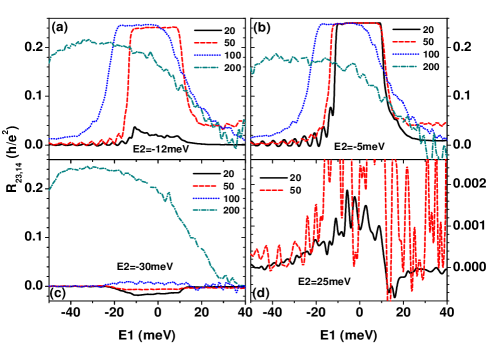
Figure 3: (Color online) $R_{23,14}$ vs on-site energy $E1$ in the injector region for different disorder strength $w=20meV$, $50meV$, $100meV$, and $200meV$. Panels (a), (b), (c), and (d) correspond to $E2=-12meV$, $-5meV$, $-30meV$ and $25meV$, respectively.

From Fig.2, we can find some common characters: (1) The Rashba SOI hardly affects the nonlocal effects of hybrid HgTe/CdTe quantum well in variant regimes (QSH-QSH, QSH-MSH, MSH-MSH regimes, and so on). For the system with $\alpha=0$ (black solid lines) and $\alpha=50meVnm$ (red dotted lines), the nonlocal resistance are almost the same, there are only slightly quantitative difference between them. So the Rashba SOI is unimportant on studying the nonlocal effect of topological insulator. (2) No matter what the values of $E2$, $R_{23,14}$ is always biggest when the injector is in the QSH regime, i.e., $E1\in[-10meV,10meV]$. This means the nonlocal effect is most remarkable in the QSH regime, that is well consistent with the experiment in Ref.[Brune et al., 2012]. (3) $R_{23,14}$ in the n-MSH and p-MSH regimes is small and shows oscillating behavior, it can even be negative for some special $E1$. Furthermore, the value of $R_{23,14}$ in the p-MSH regime is bigger than that in the n-MSH regime, as shown in the experiment.Brune et al. (2012) (4) At $E1\approx-7.5meV$, because of the finite size effect, $R_{24,13}$ abruptly peaks or dips. Now we analysis Fig.2 in detail. We focus on several main regime: the QSH-QSH regime [the central region of Fig.2(b)], the QSH-MSH regime [the left and right regions of Fig.2(b)], and the MSH-MSH regime [the left or right panel in Figs.2(c) and 2(d)]. When the injector and detector regions are all in the QSH regime (QSH-QSH hybrid regime), because of the counter propagating helical edge states, $R_{23,14}$ is biggest and is quantized at the value of $\frac{h}{4e^{2}}$, regardless of the Rashba SOI [see the central region in Fig.2(b)]. It is interpreted as follows. In the presence of the helical edge states, the transmission coefficients are integer $T_{12/21}=T_{23/32}=T_{34/43}=T_{41/14}=1$, we can then conclude $V_{2}=\frac{2}{3}V_{1}+\frac{1}{3}V_{4}$, $V_{3}=\frac{1}{3}V_{1}+\frac{2}{3}V_{4}$, and $J_{1}=-J_{4}=(4/3)(V_{1}-V_{4})$ from the Landauer-Buttiker formula. Then, $R_{23,14}=\frac{V_{2}-V_{3}}{J_{1}}=0.25h/e^{2}$. Next we consider that the energy level of the detector is $E2=-12meV$. In this case, although the Fermi energy of the detector is in the conduction band, it is very near the band edge, $10meV$, in which the bulk states coexist with edge states that leads to some exotic behaviors. We will call it the near QSH regime. When the detector is in the near QSH regime and the injector is in the QSH regime, the hybrid system will be in the near-QSH-QSH regime. In this regime, $R_{23,14}$ is decreased by the bulk states. However, the nonlocal effect is still strong [see Fig.2(a)] due to the helical edge states that survive in the bulk near band edge. Beyond the QSH-QSH regime, the MSH effects paly a role on the nonlocal transport and $R_{23,14}$ decreases because the spin Hall effect in MSH phase is weaker than that in QSH phase. In the QSH-nMSH and QSH-pMSH regimes [see left and right regions of Fig.2(b)], because the eigenstates of the MSH system are extended in the transverse directionXing et al. (2006), $R_{23,14}$ decreases rapidly and oscillates around zero. The oscillating frequency is coincident to the sub-band distribution in the conduction and valence bands. Finally, in the MSH-MSH regime [Fig.2(c,d)], the nonlocal resistance is induced by MSH completely, so $R_{23,14}$ is oscillating and very small. In this case, the nonlocal resistance $R_{23,14}$ can be negative when $E1$ is of some special values.

Figure 4: Nonlocal resistance $R_{23,14}$ vs on-site energy $E1$ in the injector region. The on-site energy in the detector region is set as $E2=-5meV$. Panels (a), (b), (c), and (d) correspond to the magnetic field $B=0$, $0.08T$, $0.16T$ and $0.32T$, respectively.

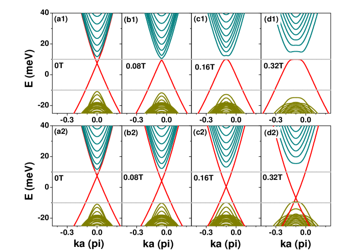
Figure 5: (Color online) Band structure of HgTe/CdTe quantum well in the presence of weak magnetic field. The bottom and top panels are for spin up and spin down, respectively. Two gray lines denote the edge of band gap in the absence of magnetic field. The on-site energy is set to zero.

Since the Rashba SOI is not important in the nonlocal effect, only the system with $\alpha=0$ is studied in the following. In Fig.3, we study the disorder effect of the nonlocal resistance $R_{23,14}$ in zero magnetic field. We choose an H-shaped scattering regions [the shadowed region in Fig.1(a)], in which the on-site potential $w_{\mathbf{i}}$ is randomly distributed in the region of $[-\frac{w}{2},\frac{w}{2}]$, with $w$ the disorder strength. When the detector (related to $E2$) is in the QSH regime [Fig.3(b)], it is possible for the system to be in the QSH-QSH, MSH-QSH and near-QSH-QSH regimes. In the presence of weak disorder ($w=20meV$), $R_{23,14}$ is quantized in the QSH-QSH regime, and the oscillating of $R_{23,14}$ in the MSH-QSH regime is strongly depressed [see the solid lines in Fig.2(b) and Fig.3(b)]. In the moderate disorder ($w=50meV$), $R_{23,14}$ in the QSH-QSH regime is still kept but $R_{23,14}$ in QSH-MSH is increased [see red dashed line in Fig.3(b)]. Besides, due to the topological Anderson insulator phenomenonXing et al. (2011); Li et al. (2009), $R_{23,14}$ in the near-QSH-QSH regime, where the detector is near QSH regime and the injector is in the QSH regime, is quantized by the moderate disorder [see the red dashed line in Fig.3(a)]. It means detector that is near QSH regime is now driven into the QSH regime by the moderate disorder. Then the disorder effect in QSH-QSH and near-QSH-QSH regime are almost same [see blue dotted lines in Fig.3(a) and Fig.3(b)]. When both $E1$ and $E2$ are far away from the energy gap, the system is in the MSH-MSH regime and $R_{23,14}$ is increased by the weak disorder [see Fig.3(d)]. When the disorder is very strong, random scattering dominates the nonlocal transport and $R_{23,14}$ in all the regimes are nearly the same [see the green dash dotted lines Fig.3(a,b,c)].

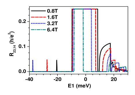
Figure 6: (Color online) Nonlocal resistance $R_{23,14}$ vs on-site energy $E1$ in the injector region for different magnetic field. The on-site energy in detector region is set as $E2=-5meV$.

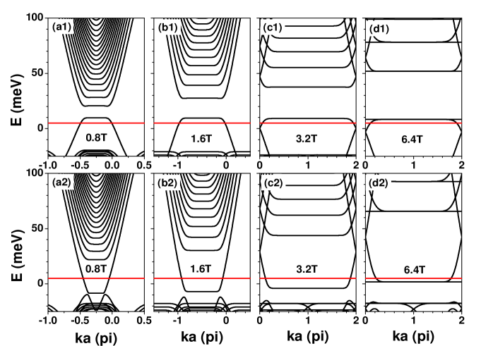
Figure 7: (Color online) Band structure of HgTe/CdTe quantum well in the presence of strong magnetic field. The bottom and top panels are for spin up and spin down, respectively. The on-site energy is set to zero. The red lines denote the position of Fermi level relative to the on-site energy.

Now, we study the nonlocal transport under the external magnetic field. We first consider the weak magnetic field. In the HgTe/CdTe quantum well, we are interested in the nonlocal properties of the helical edge states. So, in the following, we consider only the hybrid system with $E2=-5meV$, i.e., the detector is in the QSH regime. Fig.4 depicts $R_{23,14}$ vs $E1$ for different weak magnetic field $B$. The corresponding band structures are plotted in Fig.5. From Fig.4, we can find with increasing magnetic field $B$, the quantized $R_{23,14}$ in the QSH-QSH regime hardly changes and $R_{23,14}$ in the QSH-nMSH regime is suppressed gradually. This can be explained as follows. As we know, the quantized $R_{23,14}$ in the QSH-QSH regime arises from the helical edge states, while $R_{23,14}$ in the QSH-nMSH regime is dominated by the extended eigenstatesXing et al. (2006) in the MSH system. Considering the transport process, the helical edge states propagate only along the geometric edge, while the extended MSH states can propagate in the whole scattering region. Thus, when the external magnetic field is added (in all regions including the four leads and the scattering region), it can drastically affect $R_{23,14}$ in the QSH-MSH regime but hardly changes the quantized $R_{23,14}$. All in all, in the presence of weak magnetic field, it is the helical edge states and the extended MSH states that induce the unchanged quantized $R_{23,14}$ in the QSH-QSH regime and drastically suppress $R_{23,14}$ in the QSH-nMSH regime, as in the weakly disordered system. Besides, in Figs.4(b), 4(c), and 4(d), we can see that in some energy regions, e.g., $E1$ near $-10meV$ as in Fig.4(b), $E1\in[-15meV,-10meV]$ as in Fig.4(c) and $E1\in[-25meV,-10meV]$ as in Fig.4(d), except some abrupt peaks, $R_{23,14}$ is zero. This can be interpreted as follows. When the magnetic field increases, the flat Landau level forms gradually in the conduction band. The topological edge state near the conduction band gap with spin down is first broken by the magnetic field, because its chirality, i.e., the rotation direction along the scatter edge, which can be characterized by Chern number CHatsugai (1993); Sheng et al. (2006), is opposite to the edge state induced by magnetic field. The opposite chirality also induces the slight dip in Landau levels [see the top panels in Fig.5], which leads to the abrupt peaks in the conduction bandChen et al. (2012) as shown in Fig.4(c) and (d). On the other hand, for the carriers with spin up, the helical edge state near topological band gap is kept [see bottom panels in Fig.5] because its chirality is same to the Landau edge state. Combining the Landau gap in the system with spin down and the topological edge state in the system with spin up, the system is equal to a quantum Hall system, in which the edge state is unidirectional, since the edge state contributed by spin down is broken by the magnetic field. As a result, the chemical potential $V_{2}$ and $V_{3}$ of the detector terminals are determined by one of the adjacent source terminals. It means the chemical potential $V_{2}=V_{1}$ and $V_{3}=V_{2}$, which leads to zero nonlocal resistance $R_{23,14}$. Finally, there are also abrupt dips in quantized $R_{23,14}$, as interpreted in the zero magnetic field case, which comes from the finite size effect.

Next, we consider the nonlocal effect in the strong magnetic field. In this case, the edge states for spin up and spin down all develop into flat Landau levels. Fig.6 plots the nonlocal resistance $R_{23,14}$ vs on-site energy $E1$ in strong magnetic field $B$. Three characters are found: (1) Although $R_{23,14}$ is quantized in the bulk gap of [-10meV,10meV], the quantized range gradually shrinks with increasing of $B$. (2) Except several abrupt peaks, $R_{23,14}$ is nearly zero in the whole conduction band. (3) $R_{23,14}$ in the valence band is zero in some region, this region expands with increasing of $B$. To understand these behaviors, we need to analysis the band influence induced by strong magnetic field.

As we know in the HgTe/CdTe topological insulator, the chirality of the edge state induced by the inverted band is identical for electron and hole but opposite for carriers with spin up and spin down. On the other hand, in the strong magnetic field, the chirality of Landau edge state induced by the magnetic field is same for carriers with spin up and spin down but opposite for electron and hole. For all four classes of carrier, i.e., electrons and holes with spin up and spin down (signed as $e\uparrow$, $e\downarrow$, $h\uparrow$, $h\downarrow$), when the two type edge states,i.e., edge state induced by inverted band and magnetic field (signed by ‘E’ and ‘B’) have same chirality, they can coexist and boost. Otherwise, they are annihilated with each other. In our system, concerning the chirality of two types of edge states, $C_{h\uparrow,E}=C_{e\uparrow,E}=C_{e\uparrow,B}=C_{e\downarrow,B}=1$, $C_{h\uparrow,B}=C_{h\downarrow,B}=C_{h\downarrow,E}=C_{e\downarrow,E}=-1$, the edge states of $e\uparrow$ and $h\downarrow$ are strengthened, and those of $h\uparrow$ and $e\downarrow$ are destroyed in the strong magnetic field, as shown in Fig.7. However, since the edge states induced by the inverted band is more robust in the energy close to the conduction band, the destroy is more gentle (see top panels in Fig.7). So, in the strong magnetic field, the topological edge states induced by inverted band are gradually destroyed in the region of $E\in[-10meV,0]$ and nearly kept in the region of $E\in[0,10meV]$ as shown in Fig.7. And in the region of $E1\in[0,10meV]$ in Fig.6 (corresponding to $E\in[-10meV,0]$ in Fig.7), one of two helical edge states gradually disappears and the system can be regarded as a quantum Hall system with $R_{23,14}$ being zero. Then we demonstrate the first character in the last paragraph. Furthermore, in the presence of strong magnetic field, the Landau levels are completely formed in the conduction band. In the deep conduction band, the topological edge state induced by inverted band does not work and the unidirectional Landau edge states dominate the transport procession, leading to the zero $R_{23,14}$ in the conduction band of $E1<-10meV$. Besides zero $R_{23,14}$, there are also some abrupt peaks in the conduction band, it is because of the slightly dip in Landau level. This is for the second character. Finally, in the valence band, although the edge states of spin up are destroyed by the magnetic field, Landau levels have not been completely formed and there still exist extend states between Landau levels, which leads to the nonzero $R_{23,14}$ in valence band. Except these extent states, Landau levels are entirely gapped and $R_{23,14}$ is then zero. This interprets the third character in Fig.6.

Besides the three characters depicted in Fig.6, we can also expect when $B$ is large enough, the edge states of $h\uparrow$ and $e\downarrow$ are also completely destroyed, and the topological gap $[-10meV,10meV]$ in these system will become the real gap in which both the bulk and edge state are all absent.Chen et al. (2012) Then, the quantized region of $R_{23,14}$ will disappear entirely. Furthermore, when $B$ is very large, in the conduction and valence bands, the Landau edge state will dominate the transport and the system come into the quantum Hall regime, in which $R_{23,14}$ is strictly zero in any hybrid regime. So, the nonlocal resistance in the H-shaped hybrid HgTe/CdTe quantum well will completely disappear in very large magnetic field.

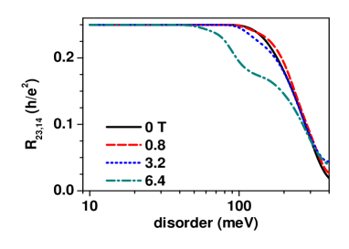
Figure 8: (Color online) Nonlocal resistance $R_{23,14}$ vs disorder strength $w$ for different magnetic field. The on-site energies of the injector and detector regions are set as $E1=E2=-5meV$.

In the following, we study the disorder effect on the nonlocal resistance in the QSH-QSH regime in the presence of strong magnetic field. We set the on-site energies in the injector and the detector as $E1=E2=-5meV$ and Fermi energy $E_{F}=0$, which equal to $E_{F}=5$ and $E1=E2=0$. With these parameters, helical QSH edge state can be maintained at very large magnetic field $B=6.4T$ [see Fig.7(d1) and (d2) in which $E_{F}=5$ and $E=0$]. However, because the magnetic field destroys the edge state in the band edge, it weakens the robustness of the helical edge state, especially for the edge states located near the gap edge, as shown in Fig.8, in which $R_{23,14}$ vs disorder strength for different magnetic field is plotted. It can be seen when $B=6.4T$, the quantized $R_{23,14}$ is decreased at small disorder strength of $w\approx 40meV$, while for $B=0$, $0.8T$ and $3.2T$, quantized $R_{23,14}$ can be maintained even at $w=100meV$. This is because at $B=6.4T$ [Fig.7(d1) and (d2)], the helical band gap is violently shrunk into the region of $[2meV,8meV]$ and $E_{F}=5meV$ is very close to the gap edge. For the magnetic field $B\leq 3.2T$, the band gap is wider of about $[-5meV,10meV]$. In this case, the Fermi energy is far away from the gap edge and the nonlocal resistance can be maintained in the strong disorder scattering.

IV conclusion

In summary, we have investigated the nonlocal transport in a H-shaped hybrid HgTe/CdTe quantum well. Three hybrid regime are considered, QSH-QSH regime, QSH-MSH regime and MSH-MSH regime. It is found in the QSH-QSH regime, the spin polarized edge states denominate the transport procession, the nonlocal effect is most strong, and the nonlocal resistance $R_{23,14}$ is quantized in the value of $0.25\frac{h}{e^{2}}$. While in the QSH-MSH device, due to the extended states in MSH effect, the nonlocal resistance is oscillating and much smaller than in the QSH-QSH device. In the MSH-MSH regime, the nonlocal effect nearly disappear, $R_{23,14}$ can only reach the order of $0.01\frac{h}{e^{2}}$. In the presence of the disorder, the quantized nonlocal resistance in the QSH-QSH device is robust because of the time reversal protected edge states. Near the QSH-QSH regime, the nonlocal resistance is enhanced and quantized due to the topological Anderson insulator phenomenon. While in the QSH-MSH and MSH-MSH device, the oscillated nonlocal resistance is strongly restricted by disorder. Finally, the magnetic field effect is investigated. It is found the quantized nonlocal resistance in QSH-QSH regime can’t be affect by weak magnetic field, but the nonlocal resistance of QSH-MSH device is smoothed out by $B$. With the increasing of $B$, the Landau level forms, counter propagating edge states are replaced by chiral edge state, so the region of quantized nonlocal resistance decrease and disappear finally. All these aforementioned nonlocal features can be derived from the special band structure of HgTe/CdTe quantum well. It is the unique property of HgTe/CdTe quantum well in topological insulator phase, it can be regarded as the fingerprint of the helical QSH edge states in 2D topological insulator.

$${\bf ACKNOWLEDGMENTS}$$

We gratefully acknowledge the financial support from the National Natural Science Foundation of China (No. 11174032 and 11274364), NBRP of China (2012CB921303), and Ph.D. Programs Foundation of Ministry of Education of China (No.20111101120024). We thank Ai-Min Guo for help discussions.
$*$ xingyanxia@bit.edu.cn
$\dagger$ qfsun@pku.edu.cn

References

- Kane and Mele (2005a) C. L. Kane and E. J. Mele, Phys. Rev. Lett. 95, 226801 (2005a), URL http://dx.doi.org/10.1103/PhysRevLett.95.226801.
- Kane and Mele (2005b) C. L. Kane and E. J. Mele, Phys. Rev. Lett. 95, 146802 (2005b), URL http://dx.doi.org/10.1103/PhysRevLett.95.146802.
- Jiang et al. (2009a) H. Jiang, S. Cheng, Q.-f. Sun, and X. Xie, Physical Review Letters 103, 036803 (2009a), URL http://dx.doi.org/10.1103/PhysRevLett.103.036803.
- Abrahams (1979) E. Abrahams, P.W. Anderson, D.C. Licciardello,and T.V. Ramakrishnan, Phys.Rev.Lett. 42, 673 (1979), URL http://dx.doi.org/10.1103/PhysRevLett.42.673.
- Li et al. (2009) J. Li, R.-L. Chu, J.K. Jain, and S.-Q. Shen, Phys. Rev. Lett. 102, 136806 (2009), URL http://dx.doi.org/10.1103/PhysRevLett.102.136806.
- Xing et al. (2011) Y. Xing, L. Zhang, and J. Wang, Phys. Rev. B 84, 035110 (2011), URL http://dx.doi.org/10.1103/PhysRevB.84.035110.
- Jiang et al. (2009) H. Jiang, L. Wang, Q.-f. Sun, and X.C. Xie, Phys. Rev. B 80, 165316 (2009), URL http://dx.doi.org/10.1103/PhysRevB.80.165316.
- Konig et al. (2007) M. Konig, S. Wiedmann, C. Brune, A. Roth, H. Buhmann, L. W. Molenkamp, X.-L. Qi, and S.-C. Zhang, Science 318, 766 (2007), URL http://dx.doi.org/10.1126/science.1148047.
- Bernevig et al. (2006) B. A. Bernevig, T. L. Hughes, and S.-C. Zhang, Science 314, 1757 (2006), URL http://dx.doi.org/10.1126/science.1133734.
- Liu et al. (2008a) C. Liu, T. Hughes, X.-L. Qi, K. Wang, and S.-C. Zhang, Physical Review Letters 100, 236601 (2008a), URL http://dx.doi.org/10.1103/PhysRevLett.100.236601.
- Knez et al. (2011) I. Knez, R.-R. Du, and G. Sullivan, Physical Review Letters 107, 136603 (2011), URL http://dx.doi.org/10.1103/PhysRevLett.107.136603.
- Knez et al. (2012) I. Knez, R.-R. Du, and G. Sullivan, Physical Review Letters 109, 186603 (2012), URL http://dx.doi.org/10.1103/PhysRevLett.109.186603.
- Yao et al. (2007) Y. Yao, F. Ye, X.-L. Qi, S.-C. Zhang, and Z. Fang, Phys. Rev. B 75, 041401 (2007), URL http://dx.doi.org/10.1103/PhysRevB.75.041401.
- Martin et al. (2008) I. Martin, Y. Blanter, and A.F. Morpurgo, Phys.Rev.Lett. 100, 036804 (2008), URL http://dx.doi.org/10.1103/PhysRevLett.100.036804.
- Roth et al. (2009) A. Roth, C. Brune, H. Buhmann, L. W. Molenkamp, J. Maciejko, X.-L. Qi, and S.-C. Zhang, Science 325, 294 (2009), URL http://dx.doi.org/10.1126/science.1174736.
- Buttiker (2009) M. Buttiker, Science 325, 278 (2009), URL http://dx.doi.org/10.1126/science.1177157.
- Brune et al. (2012) C. Brune, A. Roth, H. Buhmann, E. M. Hankiewicz, L. W. Molenkamp, J. Maciejko, X.-L. Qi, and S.-C. Zhang, Nature Physics 8, 486 (2012), URL http://dx.doi.org/10.1038/nphys2322.
- Liu et al. (2008) C.-X. Liu, X.-L. Qi, X. Dai, Z. Fang, and S.-C. Zhang, Phys. Rev. Lett. 101, 146802 (2008), URL http://dx.doi.org/10.1103/PhysRevLett.101.146802.
- Datta (Cambridge University Press, Cambridge, England, 1995) S. Datta, Electronic Transport in Mesoscopic Systems (Cambridge University Press, Cambridge, England, 1995).
- Lee and Joannopoulos (1981a) D.H. Lee and J.D. Joannopoulos, Phys. Rev. B 23, 4997 (1981a), URL http://dx.doi.org/10.1103/PhysRevB.23.4997.
- Lee and Joannopoulos (1981b) D.H. Lee and J.D. Joannopoulos, Phys. Rev. B 23, 4988 (1981b), URL http://dx.doi.org/10.1103/PhysRevB.23.4988.
- Konig et al. (2008) M. Konig, H. Buhmann, L. W. Molenkamp, T. Hughes, C.-X. Liu, X.-L. Qi, and S.-C. Zhang, J. Phys. Soc. Jpn. 77, 031007 (2008), URL http://dx.doi.org/10.1143/JPSJ.77.031007.
- Xing et al. (2006) Y. Xing, Q.-f. Sun, and J. Wang, Phys. Rev. B 73, 205339 (2006), URL http://dx.doi.org/10.1103/PhysRevB.73.205339.
- Hatsugai (1993) Y. Hatsugai, Phys. Rev. Lett. 71, 3697 (1993), URL http://link.aps.org/doi/10.1103/PhysRevLett.71.3697.
- Sheng et al. (2006) D. N. Sheng, Z. Y. Weng, L. Sheng, and F. D. M. Haldane, Phys. Rev. Lett. 97, 036808 (2006), URL http://link.aps.org/doi/10.1103/PhysRevLett.97.036808.
- Chen et al. (2012) J.-c. Chen, J. Wang, and Q.-f. Sun, Phys. Rev. B 85, 125401 (2012), URL http://link.aps.org/doi/10.1103/PhysRevB.85.125401.