A Fixed Parameter Tractable Approximation Scheme for the Optimal Cut Graph of a Surface

Abstract

Given a graph $G$ cellularly embedded on a surface $\Sigma$ of genus $g$, a cut graph is a subgraph of $G$ such that cutting $\Sigma$ along $G$ yields a topological disk. We provide a fixed parameter tractable approximation scheme for the problem of computing the shortest cut graph, that is, for any $\varepsilon>0$, we show how to compute a $(1+\varepsilon)$ approximation of the shortest cut graph in time $f(\varepsilon,g)n^{3}$.

Our techniques first rely on the computation of a spanner for the problem using the technique of brick decompositions, to reduce the problem to the case of bounded tree-width. Then, to solve the bounded tree-width case, we introduce a variant of the surface-cut decomposition of Rué, Sau and Thilikos, which may be of independent interest.

1 Introduction

Embedded graphs are commonly used to model a wide array of discrete structures, and in many cases it is necessary to consider embeddings into surfaces instead of the plane or the sphere. For example, many instances of network design actually feature some crossings, coming from tunnels or overpasses, which are appropriately modeled by a surface of small genus. In other settings, such as in computer graphics or computer-aided design, we are looking for a discrete model for objects which inherently display a non-trivial topology (e.g., holes), and graphs embedded on surfaces are the natural tool for that. From a more theoretical point of view, the graph structure theorem of Robertson and Seymour showcases a very strong connection between graphs embedded on surfaces and minor-closed families of graphs.

When dealing with embedded graphs, a classical problem, to which a lot of effort has been devoted in the past decade, is to find a topological decomposition of the underlying surface, i.e., to cut the surface into simpler pieces so as to simplify its topology, or equivalently to cut the embedded graph into a planar graph, see the recent surveys [4, 7]. This is a fundamental operation in algorithm design for surface-embedded graphs, as it allows to apply the vast number of tools available for planar graphs to this more general setting. Furthermore, making a graph planar is useful for various purposes in computer graphics and mesh processing, see for example [19]. No matter the application, a crucial parameter is always the length of the topological decomposition: having good control on it ensures that the meaningful features of the embedded graphs did not get too much distorted during the cutting.

In this article, we are interested in the problem of computing a short cut graph: For a graph $G$ with $n$ vertices embedded on a surface $\Sigma$ of genus $g$, a cut graph of $G$ is a subgraph $C\subseteq G$ such that cutting $\Sigma$ along $C$ gives a topological disk. The problem of computing the shortest possible cut graph of an embedded graph was introduced by Erickson and Har-Peled [8], who showed that it is NP-hard, provided an $n^{O(g)}$ algorithm to compute it, as well as an $O(g^{2}n\log n)$ algorithm to compute a $O(\log^{2}g)$ approximation. Now, since in most practical applications, the genus of the embedded graph tends to be quite small compared to the complexity of the graph, it is natural to also investigate this problem through the lens of parametrized complexity, which provides a natural framework to study the dependency of cutting algorithms with respect to the genus. In this direction, Erickson and Har-Peled asked whether computing the shortest cut graph is fixed-parameter tractable, i.e. whether it can be solved in time $f(g)n^{O(1)}$ for some function $f$. This question is, up to our knowledge, still open, and we address here the neighborly problem of devising a good approximation algorithm working in fixed parameter tractable time with respect to the genus; we refer to the survey of Marx [12] for more background on these algorithms at the intersection of approximation algorithms and parametrized complexity.

Our results.

In this article, we provide a fixed-parameter tractable approximation scheme for the problem of computing the shortest cut graph of an embedded graph. Namely, we prove the following theorem.

Theorem 1.1.

Let $G$ be a weighted graph cellularly embedded on a surface $\Sigma$ of genus $g$. For any $\varepsilon>0$, there exists an algorithm computing a $(1+\varepsilon)$-approximation of the shortest cut graph of $G$, which runs in time $f(\varepsilon,g)n^{3}$ for some function $f$.

Our techniques.

Our algorithm uses the brick decompositions of Borradaile, Klein and Mathieu [3] for subset-connectivity problems in planar graphs, which have been extended to bounded genus graphs by Borradaile, Demaine and Tazari [2]. Although brick decompositions are now a common tool for optimization problems for embedded graphs, it is to our knowledge the first time they are applied to compute topological decompositions. In a nutshell, the idea is the following:

1. We first compute a spanner $G_{span}$ for our problem, namely a subgraph of the input graph containing a $(1+\varepsilon)$-approximation of the optimal cut graph, and having total length bounded by $f(g,\varepsilon)$ times the length of the optimal cut graph, for some function $f$. This is achieved via brick decompositions.

2. Using a result of contraction-decomposition of Demaine, Hajiaghayi and Mohar [6], we contract a set of edges of controlled length in $G_{span}$, obtaining a graph $G_{tw}$ of bounded tree-width.

3. We use dynamic programming on $G_{tw}$ to compute its optimal cut graph.

4. We incorporate back the contracted edges, which gives us a subgraph of $G$ cutting the surface into one or more disks. Removing edges so that the complement is a single disk gives our final cut graph.

The first steps of this framework mostly follow from the same techniques as in the article of Borradaile et al. [2], the only difference being that we need a specific structure theorem to show that the obtained graph is indeed a spanner for our problem. However, as the restriction of a cut graph to a brick, i.e., a small disk on the surface, is a forest, this structure theorem is a variation of an existing theorem for the Steiner tree problem [3].

The main difficulty of this approach lies instead in the third step. Since a cut graph is inherently a topological notion, it is key for a dynamic programming approach to work with a tree-decomposition having nice topological properties. An appealing concept has been developed by Rué, Sau and Thilikos [17] for the neighborly (and for our purpose, equivalent) notion of branch-decomposition: they introduced surface-cut decompositions with this exact goal of giving a nice topological structure to work with when designing dynamic programs for graph on surfaces (see also Bonsma [1] for a related concept). However, their approach is cumbersome for our purpose when the graph embeddings are not polyhedral (we refer to the introduction for precise definitions), as it first relies on computing a polyhedral decomposition of the input graph. While dynamic programming over these polyhedral decompositions can be achieved for the class of problems that they consider, it seems unclear how to do it for the problem of computing a shortest cut graph.

We propose two ways to circumvent this issue. In the first one, we observe that the need for polyhedral embeddings in surface-cut decompositions can be traced back exclusively to a theorem of Fomin and Thilikos [17, Lemma 5.1][10, Theorem 1] relating the branch-width of an embedded graph and the carving-width of its medial graph, the proof of which uses crucially that the graph embedding is polyhedral. But another proof of this theorem which does not rely on this assumption was obtained by Inkmann [11, Theorem 3.6.1]. Therefore, the full strength of surface cut decompositions can be used without first relying on polyhedral decompositions.

However, since Inkmann’s proof is intricate and has never been published we also propose an alternative, self-contained, solution tailored to our problem. For our purpose, it is enough to make the graph polyhedral at the end of the second step of the framework while preserving a strong bound on the branch-width of the graph, we show that this can be achieved by superposing medial graphs and triangulating with care. With appropriate heavy weights on the new edges, we can ensure that they do not impact the length of the optimal cut graph and that we still obtain a valid solution to our problem.

Finally, both approaches allow us to work with a branch decomposition that possesses a nice topological structure. We then show how to exploit it to write a dynamic program to compute the shortest cut graph in fixed parameter tractable time for graphs of bounded tree-width.

Organization of the paper.

We start by introducing the main notions surrounding embedded graphs and brick decompositions in Section 2. We then prove the structure theorem in Section 3, showing that the brick decomposition with portals contains a cut graph which is at most (1+$\varepsilon$) longer than the optimal one. In Section 4, we show how to combine this structure theorem with the aforementioned framework to obtain our algorithm. This algorithm relies on one that solves the problem when the input graph has bounded tree-width, which is described in Section 5.

2 Preliminaries

All graphs $G=(V,E)$ in this article are multigraphs, possibly with loops, have $n$ vertices, $m$ edges, are undirected and their edges are weighted with a length $\ell(e)$. These weights induce naturally a length on paths and subgraphs of $G$.

Graphs on surfaces.

We will be using classical notions of graphs embedded on surfaces, for more background on the subject, we refer to the textbook of Mohar and Thomassen [14]. Throughout the article, $\Sigma$ will denote a compact connected surface of Euler genus $g$, which we will simply call genus. An embedding of $G$ on $\Sigma$ is a crossing-free drawing of $G$ on $\Sigma$, i.e. the images of the vertices are pairwise distinct and the image of each edge is a simple path intersecting the image of no other vertex or edge, except possibly at its endpoints. We will always identify an abstract graph with its embedding. A face of the embedding is a connected component of the complement of the graph. A cellular embedding is an embedding of a graph where every face is a topological disk. Every embedding in this paper will be assumed to be cellular. A graph embedding is a triangulation if all the faces have degree three. Euler’s formula states that for a graph $G$ embedded on a surface $\Sigma$, we have $n-m+f=2-g$, for $f$ the number of faces of the embedding. A noose is an embedding of the circle $\mathbb{S}^{1}$ on $\Sigma$ which intersects $G$ only at its vertices. An embedding of a graph $G$ on a surface is said to be polyhedral if $G$ is 3-connected and the smallest length of a non-contractible noose is at least 3 or if $G$ is a clique and it has at most 3 vertices. In particular, a polyhedral embedding is cellular. If $G$ is a graph embedded on $\Sigma$, the surface $\Sigma^{\prime}$ obtained by cutting $\Sigma$ along $G$ is the disjoint union of the faces of $G$, it is a (a priori disconnected) surface with boundary. When we cut a surface along a set of nooses, viewed as a graph, the resulting connected components will be called regions. A combinatorial map of an embedded graph is the combinatorial description of its embedding, namely the cyclic ordering of the edges around each vertex.

Given an embedded graph $G$, the medial graph $M_{G}$ is the embedded graph obtained by placing a vertex $v_{e}$ for every edge $e$ of $G$, and connecting the vertices $v_{e}$ and $v_{e}^{\prime}$ with an edge whenever $e$ and $e^{\prime}$ are adjacent on a face of $G$. The barycentric subdivision of an embedded graph $G$ is the embedded graph obtained by adding a vertex on each edge and on each face and an edge between every such face vertex and its adjacent (original) vertices and edge vertices.

For $\Sigma$ a surface and $G$ a graph embedded on $\Sigma$, a cut graph of $(\Sigma,G)$ is a subgraph $H$ of $G$ whose unique face is a disk. The length of the cut graph is the sum of the lengths of the edges of $H$. Throughout the whole paper, OPT will denote the length of the shortest cut graph of $(\Sigma,G)$.

We refer the reader to [2, 17] for definitions pertaining to tree decomposition and branch decomposition. A carving decomposition of a graph $G$ is the analogue of a branch decomposition with vertices and edges inverted, with the carving-width defined analogously. A bond carving decomposition is a special kind of carving decomposition where the middle sets always separate the graph in two connected components. Since these concepts only appear sporadically in this paper, we refer to [17] for a precise definition.

Mortar graph and bricks.

The framework of mortar graphs and bricks has been developed by Borradaile, Klein and Mathieu [3] to efficiently compute spanners for subset connectivity problems in planar graphs. We recall here the main definitions around mortar graphs and bricks and refer to the articles [2, 3] for more background on these objects.

Let $G$ be a graph embedded on $\Sigma$ of genus $g$. A path $P$ in a graph $G$ is $\varepsilon$-short in $G$ if for every pair of vertices $x$ and $y$ on $P$, the distance from $x$ to $y$ along $P$ is at most $(1+\varepsilon)$ times the distance from $x$ to $y$ in $G$: $\textrm{dist}_{P}(x,y)\leq(1+\varepsilon)\textrm{dist}_{G}(x,y)$. For $\varepsilon>0$, let $\kappa(g,\varepsilon)$ and $\alpha(g,\varepsilon)$ be functions to be defined later. A mortar graph $MG(G,\varepsilon)$ is a subgraph of $G$ such that $\ell(MG)\leq\alpha OPT$, and the faces of $MG$ partition $G$ into bricks $B$ that satisfy the following properties:

1. $B$ is planar.

2. The boundary of $B$ is the union of four paths in clockwise order $N,E,S$, $W$.

3. $N$ is $0$-short in $B$, and every proper subpath of $S$ is $\varepsilon$-short in $B$.

4. There exists a number $k\leq\kappa$ and vertices $s_{0}\ldots s_{k}$ ordered from left to right along $S$ such that, for any vertex $x$ of $S[s_{i},s_{i+1})$, $\textrm{dist}_{S}(x,s_{i})\leq\varepsilon\textrm{dist}_{B}(x,N)$.

The mortar graph is computed using a slight variant of the procedure in [2, Theorem 4], the idea is the following:

1. Cut $\Sigma$ along an approximate cut graph, yielding a disk $D$ with boundary $\partial D$.

2. Find shortest paths between certain vertices of $\partial D$. This defines the $N$ and $S$ boundaries of the bricks.

3. Find shortest paths between vertices of the previous paths. These paths are called the columns.

4. Take every $\kappa$th path found in the last step. These paths are called the supercolumns and form the $E$ and $W$ boundaries of the bricks. The constant $\kappa$ is called the spacing of the supercolumns.

This leads to the following theorem to compute the mortar graph in time $O(g^{2}n\log n)$.

Theorem 2.1.

Let $\varepsilon>0$ and $G$ be a graph embedded on $\Sigma$ of genus $g$. There exists $\alpha=O(\log^{2}g\varepsilon^{-1})$ such that there is a mortar graph $MG(G,\varepsilon)$ of $G$ such that $\ell(MG)\leq\alpha OPT$ and the supercolumns of $MG$ have length $\leq\varepsilon OPT$ with spacing $\kappa=O(\log^{2}g\varepsilon^{-3})$. This mortar graph can be found in $O(g^{2}n\log n)$ time.

The proof of Theorem 2.1 relies on the following planar construction of the mortar graph obtained by Borradaile, Klein and Mathieu [3] (we cite the version of Borradaile, Demaine and Tazari [2, Theorem 2].)

Theorem 2.2.

Let $\varepsilon>0$ and $G$ be a planar graph with outer face $H$, such that $\ell(H)\leq\alpha_{0}OPT$, for some $\alpha_{0}$. For $\alpha=(2\alpha_{0}+1)\varepsilon^{-1}$, there is a mortar graph $MH(G,\varepsilon)$ containing $H$ whose length is at most $\alpha OPT$ and whose supercolumns have length $\varepsilon OPT$ with spacing $\kappa=\alpha_{0}\varepsilon^{-2}(1+\varepsilon^{-1})$. The mortar graph can be found in $O(n\log n)$ time.

Proof of Theorem 2.1.

The proof of this theorem follows closely the one in [2]. The main difference is that the value of OPT is different, therefore we use a different cutting strategy from the start.

We first compute an $O(\log^{2}g)$ approximation of the optimal cut graph using the algorithm in of Erickson and Har-Peled [8] and cut along it, to obtain a planar graph $H$. We can now apply Theorem 2.2 to $H$ to obtain a mortar graph of $H$, and it is easy to verify that it is a mortar graph of $G$ as well. The theorem follows from the bounds of Theorem 2.2 and the $O(\log^{2}g)$ approximation, the bottleneck of the complexity being the computation of the approximation of the cut graph. ∎

3 Structure Theorem

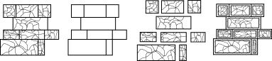
Figure 1: The different stages of the brick decomposition of a graph $G$, the mortar graph, the set of bricks and the graph $B^{+}(MG,\theta)$.

In this section, we prove the structure theorem, which shows that there exists an $\varepsilon$-approximation to the optimal cut graph which only crosses the mortar graph at a small subset of vertices called portals.

In order to state this theorem, following the literature, we define a brick-copy operation $B^{+}$ as follows. For each brick $B$, a subset of $\theta$ vertices is chosen as portals such that the distance along $\partial B$ between any vertex and the closest portal is at most $\ell(\partial B)/\theta$. For every brick $B$, embed $B$ in the corresponding face of $MG$ and connect every portal of $B$ to the corresponding vertex of $MG$ with a zero-length portal edge; this defines $B^{+}(MG,\theta)$. The edges originating from $MG$ are called the mortar edges.

We note that by construction, $B^{+}(MG,\theta)$ embeds on the plane in such a way that every brick of $B^{+}(MG,\theta)$ is included in the corresponding brick of $MG$. Furthermore, every vertex of $G$ corresponds to a vertex of $B^{+}(MG,\theta)$ by mapping the insides of bricks to the insides of bricks in $B^{+}(MG,\theta)$, and the mortar graph to itself, cf. Figure 1. We denote this map by $i:V(G)\rightarrow V(B^{+}(MG,\theta))$.

Moreover, we contract the $E$ and $W$ boundaries of each brick of $B^{+}(MG,\theta)$ and their copies in the mortar graph. Since the sum of the length of the $E$ and $W$ boundaries is at most $\varepsilon OPT$, any solution of length $\ell$ in $B^{+}(MG,\theta)$ going through a vertex resulting from a contraction can be transformed into a solution of length at most $\ell+2\varepsilon OPT$ in $B^{+}(MG,\theta)$ where no edge is contracted. The structure theorem is then the following:

Theorem 3.1.

Let $G$ be a graph embedded on $\Sigma$ of genus $g$, and $\varepsilon>0$. Let $MG(G,\varepsilon)$ be a corresponding mortar graph of length at most $\alpha OPT$ and supercolumns of length at most $\varepsilon OPT$ with spacing $\kappa$. There exists a constant $\theta(\alpha,\varepsilon,\kappa)$ depending polynomially on $\alpha,1/\varepsilon$ and $\kappa$ such that:

$$\textrm{OPT}(B^{+}(MG,\theta))\leq(1+c\varepsilon)\textrm{OPT}.$$

The proof of this theorem essentially consists in plugging in the structure theorem of [3] and verifying that it fits. Let us first recall the structural theorem of bricks [3]. For a graph $H$ and a path $P\subseteq H$, a joining vertex of $H$ with $P$ is a vertex in $P$ that lies on an edge of $H\setminus P$.

Theorem 3.2.

[3, Theorem 10.7] Let $B$ be a brick, and $F$ be a set of edges of $B$. There is a forest $\widetilde{F}$ in $B$ with the following properties:

1. If two vertices of $N\cup S$ are connected by $F$, they are also connected by $\widetilde{F}$,

2. The number of joining vertices of $\widetilde{F}$ with both $N$ and $S$ is bounded by $\gamma(\kappa,\varepsilon)$,

3. $\ell(\widetilde{(}F))\leq\ell(F)(1+c\varepsilon)$.

   In the above, $\gamma(\kappa,\varepsilon)=o(\varepsilon^{-2.5}\kappa)$ and $c$ is a fixed constant.

From this we can deduce the following proposition.

Proposition 3.3.

Let $C$ be a subgraph of $G$ of length $OPT$. There exists a constant $\theta(\alpha,\varepsilon,\kappa)$ depending polynomially on $\alpha,1/\varepsilon$ and $\kappa$ and a subgraph $\widehat{C}$ of $B^{+}(MG,\theta)$ with the following properties:

• $\ell(\widehat{C})\leq(1+\tilde{c}\varepsilon)\ell(C)=(1+\tilde{c}\varepsilon)OPT$, where $\tilde{c}$ is a fixed constant.

• If we denote by $D$ the closed disk on which $MG$ has been constructed, for any two vertices $s,t\in\partial D$ that are connected by $C$ in $D$, $i(s)$ and $i(t)$ are connected by $\widehat{C}$ in $D$ as well.

Proof.

We recall that the interior of every brick $B$ of $G$ can naturally be embedded in the corresponding brick of $B^{+}(MG,\theta)$, therefore, for every brick $B$, we can identify $C\cap B$ with a subgraph of $B^{+}(MG,\theta)$. We define $\widehat{C}$ as follows:

• For every edge of $C$ which is an edge of the mortar graph $MG$, we add the corresponding mortar edge in $B^{+}(MG,\theta)$ to $\widehat{C}$.

• In the inside of every brick $B$, if $F$ is the forest induced by $C\cap B$, we define $\widehat{C}\cap B$ to be the forest defined by $\widetilde{F}$ (as defined in Theorem 3.2)

• Finally, for every brick $B$, let $Q(B)$ denote the set of joining vertices of $\widetilde{C}$ with $N\cup S$. For every vertex of $Q(B)$ in a brick $B$, we add to $\widetilde{C}$ the path to its closest portal, the copy of this path in the mortar graph, as well as the corresponding portal edge.

We start by proving the first property. The length of $\widehat{C}$ restricted to $B$ is at most $(1+c\varepsilon)$ times the length of $C$ restricted to $B$. The length incurred by the portal operation is

$$\sum\limits_{B}\sum\limits_{q\in Q(B)}\leq 2\sum\limits_{B}|Q(B)|\frac{\ell(\partial B)}{\theta}\leq 2\sum\limits_{B}\gamma(\varepsilon)\frac{\ell(\partial B)}{\theta}.$$

By defining $\theta=\gamma(\varepsilon)\alpha\varepsilon^{-1}$ portals, we obtain that the length of $\widehat{C}$ is at most $(1+c^{\prime}\varepsilon)OPT$ for some universal constant $c^{\prime}$, since the length of the mortar graph is at most $\alpha OPT$.

We now prove the second property. Consider two vertices $u,v$ on $\partial D$ that are connected in $C$ and let $P$ be the path in $C$ connecting them. Recall that any vertex that belongs to $\partial D$ belongs to the mortar graph. We decompose $P$ into subpaths crossing at most one brick and whose extremities lie on the mortar graph. For any such subpath $s=\{s,\ldots,t\}$ in a brick $B$, we show that there exists a path in $\widehat{C}$ connecting $i(s)$ to $i(t)$. We consider the set of vertices $s_{B}:=Q(B)\cap s$. By definition of $\widehat{C}$, $i(s)$ and $i(t)$ are connected to vertices of $s_{B}$. Property 1 of Theorem 3.2 implies that for any couple of vertices of $Q(B)$, if they are connected in $C$ they are also connected in $\widehat{C}$. Therefore, we conclude that $i(s)$ and $i(t)$ are connected and therefore $u$ and $v$ are also connected.

∎

We now have all the tools to prove the structure theorem.

Proof of Theorem 3.1.

Let $C$ be an optimal cut graph of $(\Sigma,G)$. We apply Proposition 3.3 to $C$, it yields a subgraph $\widehat{C}$ of $B^{+}(MG,\theta)$ of length $\ell(\widehat{C})\leq(1+\varepsilon)\ell(C)$. We claim that this graph $\widehat{C}$ contains a cut graph of $\Sigma$.

Suppose on the contrary that there exists a non-contractible cycle $\gamma$ in $(\Sigma,B^{+}(MG,\theta))$ which does not cross $\widehat{C}$. This cycle $\gamma$ corresponds to a cycle $\gamma^{\prime}$ in $(\Sigma,G)$ by contracting portal edges, and since $C$ is a cut graph, there exists a maximal subpath $P$ of $C$ restricted to $D$ and a maximum subpath $P^{\prime}$ of $\gamma^{\prime}$ in $D$ such that $P^{\prime}$ crosses $P$ an odd number of times, otherwise, by flipping bigons we could find a cycle homotopic to $\gamma^{\prime}$ not crossing $C$. Denote by $(s,t)$ and $(s^{\prime},t^{\prime})$ the intersections of $P$ and $P^{\prime}$ with $\partial D$. Then, without loss of generality, $s$, $s^{\prime}$, $t$ and $t^{\prime}$ appear in this order on $\partial D$. Furthermore, the vertices $i(s)$ and $i(t)$ in $B^{+}(MG,\theta)$ are connected by $\widehat{C}$ by Proposition 3.3, since $s$ and $t$ are connected by $C$. Therefore, $\gamma$ crosses $\widehat{C}$, and we reach a contradiction. ∎

4 Algorithm

We now explain how to apply the spanner framework of Borradaile et al. in [2] to compute an approximation of the optimal cut graph. We start by computing the optimal Steiner tree, for each subset of the portals in every brick by using the algorithm or Erickson, Monma, and Veinott  [9], and then take the union of all these trees over all bricks, plus the edges of the mortar graph. As this algorithm runs in time $O(nk^{3})$, this step takes time $O_{g,\varepsilon}(n)$. This defines the graph $G_{span}$, which by construction has length $\leq f(g,\varepsilon)OPT$, where $f(g,\varepsilon)=O(2^{\theta})=2^{O(\log^{2}g)poly(1/\varepsilon)}$, and contains a $(1+\varepsilon)$ approximation of the optimal cut graph by the structure theorem.

We will use the following theorem of Demaine et al. [6, Theorem 1.1] (the complexity of this algorithm can be improved to $O_{g}(n)$ [5]).

Theorem 4.1.

For a fixed genus $g$, any $k\geq 2$ and any graph $G$ of genus at most $g$, the edges of $G$ can be partitioned into $k$ sets such that contracting any one of the sets results in a graph of tree-width at most $O(g^{2}k)$. Furthermore, the partition can be found in time $O(g^{5/2}n^{3/2}\log n)$ time.

The four steps of the framework are now the following.

1. Compute the spanner $G_{span}$.

2. Apply Theorem 4.1 with $k=f(g,\varepsilon)/\varepsilon$, and contract the edges in the set of the partition with the least weight. The resulting graph $G_{tw}$ has tree-width at most $O(g^{2}\varepsilon^{-1}f(g,\varepsilon))$.

3. Use the bounded tree-width to compute a cut graph of $(\Sigma,G_{tw})$. An algorithm to do this is described in Section 5.

4. Incorporate the contracted edges back. By definition, they have length at most $f(g,\varepsilon)OPT/k=\varepsilon OPT$. Therefore, the final graph we obtain has the desired length. If the resulting graph has more than one face, remove edges until we obtain a cut-graph.

We now analyze the complexity of this algorithm. The spanner is computed in time $O_{g,\varepsilon}(n\log n)$. Using [5], the second step takes time $O_{g,\varepsilon}(n)$. Dynamic programming takes time $O_{g,\varepsilon}(n^{3})$ (see thereafter), and the final lifting step takes linear time. Assuming the dynamic programming step described in the next section, this proves Theorem 1.1.

5 Computing cut graphs for bounded tree-width

There remains to prove that computing the optimal cut graph of $(\Sigma,G)$ is fixed parameter tractable with respect to both the tree-width of $G$ and the genus of $\Sigma$ as a parameter. Out of convenience, we work with the branch-width instead, which gives the result since they are within a constant factor [16, Theorem 5.1]. As cut graphs are a topological object, we will rely on surface-cut decompositions [17], which are a topological strengthening of branch decompositions. Note that, for reasons which will be clear later, our definition is slightly different from the one of Rué, Sau and Thilikos as it does not rely on polyhedral decompositions.

Given a graph $G$ embedded in a surface $\Sigma$ of genus $G$, a surface-cut decomposition of $G$ is a branch decomposition $(T,\mu)$ of $G$ such that for each edge $e\in E(T)$, the vertices in $\textrm{mid}(e)$ are contained in a set $\mathcal{N}$ of nooses in $\Sigma$ such that:

• $|\mathcal{N}|=O(g)$

• The nooses in $\mathcal{N}$ pairwise intersect only at subsets of $\textrm{mid}(e)$

• $\theta(\mathcal{N})=O(g)$

• $\Sigma\setminus\bigcup\mathcal{N}$ contains exactly two connected components, of which closures contain respectively $G_{1}$ and $G_{2}$.

where $\theta$ is defined as follows: for a point $p$ in $\Sigma$, if we denote by $\mathcal{N}(p)$ the number of nooses in $\mathcal{N}$ containing $p$, and let $P(\mathcal{N})=\{p\in\Sigma\mid\mathcal{N}(p)\geq 2\}$, we define

$$\theta(\mathcal{N})=\sum_{p\in P(\mathcal{N})}\mathcal{N}(p)-1.$$

Rué et al. showed how to compute such a surface-cut decomposition when the input graph $G$ is embedded polyhedrally on the surface $\Sigma$:

Theorem 5.1 ([17, Theorem 7.2]).

Given a graph $G$ on $n$ vertices polyhedrally embedded on a surface of genus $g$ and with $bw(G)\leq k$, one can compute a surface-cut decomposition of $G$ of width $O(g+k)$ in time $2^{O(k)}n^{3}$.

When the input graph is not polyhedral, Rué et al. propose a more intricate version of surface-cut decompositions relying on polyhedral decompositions, but it is unclear how to incorporate these in a dynamic program to compute optimal cut graphs.

Instead, we present two ways to circumvent polyhedral decompositions and use these surface-cut decompositions directly. The first one consists of observing that the difficulties involved with computing surface-cut decompositions of non-polyhedral embeddings can be circumvented by using a theorem of Inkmann [11]. Since Inkmann’s theorem has, up to our knowledge, not been published outside of his thesis, and the proof is quite intricate, for the sake of clarity we also provide a different approach, based on modifying the input graph to make it polyhedral.

In both cases, we obtain a branch decomposition with a strong topological structure, which we can then use as a basis for a dynamic program to compute the optimal cut graph.

5.1 A simpler version of surface-cut decompositions

The algorithm [17, Algorithm 2] behind the proof of Theorem 5.1 relies on the following steps. Starting with a polyhedral embedding of $G$ on a surface,

1. Compute a branch decomposition branch(G) of $G$.

2. Transform branch(G) into a carving decomposition carv(G) of $M_{G}$.

3. Transform carv(G) into a bond carving decomposition bond(G) of $M_{G}$.

4. Transform bond(G) into a branch decomposition of $G$.

The second step is the only one where where the polyhedrality of the embedding is used, as it relies on the following lemma:

Lemma 5.2 ([17, Lemma 5.1]).

Let $G$ be a polyhedral embedding on a surface $\Sigma$ of genus $g$, and $M_{G}$ be the embedding of the medial graph. Then $bw(G)\leq cw(M_{G})/2\leq 6bw(G)+4g+O(1)$, and the corresponding carving decomposition of $M_{G}$ can be computed from the branch decomposition of $G$ in linear time.

We observe that the following theorem of Inkmann shows that the branch-width of a surface-embedded graph and the carving-width of its medial graph are tightly related, even for non-polyhedral embeddings.

Theorem 5.3 ([11, Theorem 3.6.1]).

For every surface $\Sigma$ there is a non-negative constant $c(\Sigma)$ such that if $G$ is embedded on $\Sigma$ with $|E(G)|\geq 2$ and $M_{G}$ is its medial graph, we have $2bw(G)\leq cw(M)\leq 4bw(G)+c(\Sigma).$

Digging into the proof reveals that $c(\Sigma)=O(g^{2})$ for $\Sigma$ of genus $g$. The idea is therefore that replacing Lemma 5.1 of Rué et al. by Theorem 5.3 allows us to lift the requirement of polyhedral embedding in their construction. One downside is that this theorem does not seem to be constructive, and therefore we need an alternative way to compute the carving decomposition in step 2. This can be achieved in fixed parameter tractable time with respect to the carving-width (and linear in $n$) using the algorithm of Thilikos, Serna and Bodlaender [18]. In conclusion, we obtain the following corollary (note that the bottleneck in the complexity is the same as in the one of Rué et al., which is the transformation between a carving and a bond carving decomposition).

Corollary 5.4.

Given a graph $G$ on $n$ vertices embedded in a surface of genus $g$ with $\textrm{bw}(G)\leq k$, there exists an algorithm running in time $O_{k}(n^{3})$ computing a surface-cut decomposition $(T,\mu)$ of $G$ of width at most $O(k+g^{2})$.

5.2 Making a graph polyhedral

In this section, we show how to go from an embedded graph to a polyhedral embedding, without increasing the tree-width too much. The construction will be split in the following three lemmas.

Lemma 5.5.

Let $G$ be a graph of tree-width at most $k\geq 2$, embedded on a surface of genus $g$. Then there exists a triangulation of $G$ of tree-width at most $k$. Moreover, given a tree-decomposition of width $k$, one can compute a triangulation of $G$ of tree-width at most $k$ in polynomial time.

Proof.

Let $\widetilde{G}$ be the chordal graph containing $G$ having the smallest clique number, i.e., $k+1$. We just observe that $\widetilde{G}$ contains a triangulation of $G$, which will therefore have the same treewidth as $G$.

We now show how to compute a triangulation of tree-width $k$ given a tree-decomposition $\mathcal{T}$ of width $k$. Consider the graph $\widetilde{G}$ which consists of $G$ plus all the edges connecting the vertices $u,v$ that are present in the same bag of $\mathcal{T}$. By definition of the tree-decomposition, $\widetilde{G}$ is chordal and has the same tree-width than $G$. Then, for any cycle of $G$ of length at least 4, there exists a bag which induces at least one chord, namely such that adding all the edges between the vertices of the bag creates a chord in the cycle. Therefore, we can proceed greedily and for each face $f$ of length at least 4 of $G$, find a bag that contains two non-consecutive vertices of $f$, add this edge to $G$, embed it in the face and proceed recursively. ∎

Lemma 5.6.

Let $G$ be a triangulated graph of tree-width at most $k$, embedded on a surface of genus $g$. Then its barycentric subdivision $B(G)$ has tree-width at most $f(k,g)$ for some function $f$.

Proof.

The barycentric subdivision consists of the original vertices of $G$, the edge vertices and the face vertices. Let $G_{e}$ be the barycentric subdivision of $G$ restricted to the face and edge vertices, namely $G_{e}$ consists in the dual of $G$ where each edge is subdivided. Let $T=(X_{1}\ldots X_{n})$ be a tree decomposition of $G_{e}$. By [13], the size of the bags of $T$ is bounded by some function $h(k,g)$. We consider the tree-decomposition $T^{\prime}=(X_{1}^{\prime}\ldots X_{n}^{\prime})$ of $B(G)$ obtained by adding an original vertex to every bag $X_{i}$ containing at least one of its neighbors in its barycentric subdivision, namely an adjacent face or edge vertex. Since $G$ is triangulated, the size of the bags is multiplied by at most a constant. Let us prove that $T^{\prime}$ is a tree decomposition:

• It contains all the vertices of $B(G)$.

• For every edge, there is a bag containing both endpoints.

• Let $X_{i}^{\prime}$ and $X_{j}^{\prime}$ be two bags containing a vertex $v$. If $v$ is a face or an edge vertex, every bag on the path between $X^{\prime}_{i}$ and $X^{\prime}_{j}$ contains it. If it is an original vertex, then $X^{\prime}_{i}$ and $X^{\prime}_{2}$ both contain a neighbor of $v$, which we denote by $v_{1}$ and $v_{2}$. Now, if there is a bag $X^{\prime}_{k}$ on the path between $X^{\prime}_{i}$ and $X^{\prime}_{j}$ which does not contain $v$, it does not contain any neighbor of $v$ either, but it separates $v_{1}$ from $v_{2}$ in $B(G)$. We have reached a contradiction.

∎

Lemma 5.7.

Let $G$ be a triangulated graph of tree-width at most $k$, embedded on a surface of genus $g$. Let $M_{G}$ denote the medial graph of $G$, and $G^{\prime}$ the superposition of $G$ and $M_{G}$. Then the tree-width of $G^{\prime}$ is bounded by some function of $k$ and $g$.

Proof.

The idea of the proof is the same as for the previous lemma. We start with a tree decomposition $T=(X_{1}\ldots X_{n})$ of $M_{G}$. Since $M_{G}$ is the dual of the radial graph of $G$, which is contained in the barycentric subdivision of $G$, by the previous lemma and [13], the treewidth of $M_{G}$ is bounded by some function of $k$ and $g$. Now, define $T^{\prime}=(X^{\prime}_{1}\ldots X^{\prime}_{n})$ by adding every original vertex in $G^{\prime}$ to the bags of $T$ containing any of its neighbors. The size of the bags at most triple in size, and let us prove that $T^{\prime}$ is a tree decomposition:

• It contains all the vertices of $G^{\prime}$.

• For every edge, there is a bag containing both endpoints.

• Let $X_{i}^{\prime}$ and $X_{j}^{\prime}$ be two bags containing a vertex $v$. If $v$ is a vertex of $M_{G}$, every bag on the path between $X^{\prime}_{i}$ and $X^{\prime}_{j}$ contains it. If it is an original vertex, then $X^{\prime}_{i}$ and $X^{\prime}_{2}$ both contain a neighbor of $v$, which we denote by $v_{1}$ and $v_{2}$. Now, if there is a bag $X^{\prime}_{k}$ on the path between $X^{\prime}_{i}$ and $X^{\prime}_{j}$ which does not contain $v$, it does not contain any neighbor of $v$ either, but it separates $v_{1}$ from $v_{2}$ in $G^{\prime}$. We have reached a contradiction.

∎

Now, we observe that superposing medial graphs two times increases the length of non-contractible nooses of a graph. Furthermore, if the new edges are weighted heavily enough (e.g., with a weight larger than OPT, which we know how to approximate), they will not change the value of the optimal cut graph. Therefore this allows us to assume that the embedded graph of which we want to compute an optimal cut graph has only non-contractible nooses of length at least three. By subdividing it to remove loops and multiple edges and triangulating it, we can also assume that it is 3-connected (since the link of every vertex of a triangulated simple graph is 2-connected), and therefore that it is polyhedral.

For a polyhedral embedding, our definition of surface-cut decompositions and the one of Rué et al. [17] coincide, and therefore we can use their algorithm to compute it.

5.3 Dynamic programming on surface-cut decompositions

We now show how to compute an optimal cut graph of an embedded graph of bounded branch-width, using surface-cut decompositions. We first recall the following lemma of Erickson and Har-Peled which follows from Euler’s formula and allows us to bound the complexity of the optimal cut graph. For a graph $H$ embedded on a region $R$, we define its reduced graph to be the embedded graph obtained by repeatedly removing from $G$ the degree 1 vertices which are not on a boundary and their adjacent edges, and contracting each maximal path through degree 2 vertices to a single edge (weighted as the length of the path).

Lemma 5.8 ([8, Lemma 4.2]).

Let $\Sigma$ be a surface of genus $g$. Then any reduced cut graph on $\Sigma$ has less than $4g$ vertices and $6g$ edges.

The idea is then to compute in a dynamic programming fashion, for every region $R$ of the surface-cut decomposition, every possible combinatorial map $M$ corresponding to the restriction of a reduced cut graph of $\Sigma$ to $R$, and every possible position $P$ of the vertices of the boundary of $M$ on the boundary of $R$, the shortest reduced graph embedded on $R$ with map $M$ and position $P$. The bounds on the size of the boundaries of the region (coming from the definition of surface-cut decompositions), as well as Lemma 5.8 allow us to bound the size of the dynamic tables.

Theorem 5.9.

If a graph $G$ of complexity $n$ embedded on a genus $g$ surface has branch-width at most $k$, an optimal cut graph of $G$ can be computed in time $O_{g,k}(n^{3})$.

Proof of Theorem 5.9.

We start by computing a surface-cut decomposition $(T,\mu)$ of $(\Sigma,G)$ using either of the algorithms presented in Section 5, and the width of $(T,\mu)$ is $O(g^{2}+k)$.

Then, our algorithm relies on dynamic programming. For every edge $e$ in the tree of the surface-cut decomposition, there is a set of nooses $\mathcal{N}_{e}$, such that cutting $\Sigma$ along $\mathcal{N}_{e}$ yields two connected regions $R_{1}$ and $R_{2}$ of $\Sigma$. The set of nooses $\mathcal{N}_{e}$ contains exactly $mid(e)$ vertices, but every vertex appearing multiple times in $\mathcal{N}_{e}$ gets copied as many times when considered on the boundary of $R_{1}$ or $R_{2}$. However, since $\theta(\mathcal{N}_{e})=O(g)$, this only happens $O(g)$ times at most, and therefore the boundary of $R_{1}$ (or $R_{2}$) contains $O(g+mid(e))=O(g^{2}+k)$ vertices.

For any region $R$ of the surface-cut decomposition, a reduced cut graph $C$ of $(\Sigma,G)$ induces a combinatorial map $M$ on $R$. We denote by $\mathcal{M}(R)$ the set of all these maps, for all the reduced cut graphs of $(\Sigma,G)$. For a map $M$ in $\mathcal{M}(R)$, the vertices of $M$ on the boundary of $R$ are called its boundary vertices. Any embedded graph on $R$ with map $M$ induces a matching between the boundary vertices of $M$ and the vertices on the boundary of $R$, and the set of all these possible matchings is called the set $\mathcal{P}(M,R)$ of boundary positions of $M$ in $R$.

The reduced combinatorial map of an embedded graph is the combinatorial map of its reduced graph. For every region $R$ induced by the surface-cut decomposition, every combinatorial map $M$ in $\mathcal{M}(R)$ and every boundary position $P\in\mathcal{P}(M,R)$, the dynamic programming tables store a number $T[R,M,P]$ which is the length of the shortest subgraph of $G$ in $R$ with reduced combinatorial map $M$ and with boundary positions $P$. Given a region $R$ and its two subregions $R_{1}$ and $R_{2}$, the data of the dynamic programming tables of $R_{1}$ and $R_{2}$ allow to compute the table of $R$ by the following formula:

$$T[R,M,P]=\min_{M_{1},M_{2}\in\mathcal{S}(M,R_{1},R_{2})}\min_{P_{1},P_{2}\in\mathcal{T}(M_{1},M_{2},P)}T[R_{1},M_{1},P_{1}]+T[R_{2},M_{2},P_{2}],$$

where $\mathcal{S}(M,R_{1},R_{2})\subseteq\mathcal{M}(R_{1})\times\mathcal{M}(R_{2})$ is the set of combinatorial maps in $R_{1}$ and $R_{2}$, which glued together give the map $M$ on $R$, and $\mathcal{T}(M_{1},M_{2},P)\subseteq\mathcal{P}(M_{1},R_{1})\times\mathcal{P}(M_{2},R_{2})$ is the set of boundary positions of $M_{1}$ in $R_{1}$ and $M_{2}$ in $R_{2}$ such that vertices glued together on the boundary of $R_{1}$ and $R_{2}$ are mapped to the same vertex and vertices on the boundary of $R$ are mapped according to $P$. As usual, the minimum is taken to be infinite if the sets are empty.

We now bound the size of the tables. For a region $R$, the set $\mathcal{M}(R)$ consists of combinatorial maps having at most $4g$ vertices of degree at least 3 (by Lemma 5.8), no vertices of degree 2 (since they have been contracted during the reduction), and vertices of degree 1 only on the boundary of $R$. Since the number of vertices on the boundary of $R$ is $O(g^{2}+k)$, the size of $\mathcal{M}(R)$ is bounded by a function of $g$ and $k$. Similarly, the size of $\mathcal{P}(M,R)$ is bounded by a function depending on the number of boundary vertices of $M$ and $R$, and thus by a function of only $g$ and $k$.

Finally, the length of the optimal reduced cut graph is equal to the minimum of $T[\Sigma,M,\emptyset]$, where $M$ ranges over all the combinatorial maps of reduced cut graphs on $\Sigma$. The number of such combinatorial maps is bounded a function of $g$ by Lemma 5.8. The complexity of the dynamic program is therefore $O_{g,k}(n^{3})$, where the cubic dependency comes from the computation of the surface-cut decomposition. Since, when doing a reduction, removing the degree 1 vertices not on the boundary only reduces the length, the length of the optimal reduced cut graph is the same as the length of the optimal cut graph. This concludes the proof.

∎

Open problems.

One of the main challenges is whether the problem of computing the shortest cut graph can be solved exactly in FPT complexity – the recent application of brick decompositions to exact solutions for Steiner problems [15] might help in this direction. In the approximability direction, it is also unknown whether there exists a polynomial time constant factor approximation to this problem, or even a PTAS.

Acknowledgments

We are grateful to Sergio Cabello, Éric Colin de Verdière, Frederic Dorn and Dimitrios M. Thilikos for very helpful remarks at various stages of the elaboration of this article.

References

- [1] P. Bonsma, Surface split decompositions and subgraph isomorphism in graphs on surfaces, in Proc. of the Symp. on Theoretical Aspects of Computer Science, STACS ’12, 2012, pp. 531–542.
- [2] G. Borradaile, E. D. Demaine, and S. Tazari, Polynomial-time approximation schemes for subset-connectivity problems in bounded-genus graphs, Algorithmica, 68 (2014), pp. 287–311.
- [3] G. Borradaile, Ph. N. Klein, and C. Mathieu, An approximation scheme for Steiner tree in planar graphs, ACM Trans. on Algorithms, 5 (2009).
- [4] É. Colin de Verdière, Topological algorithms for graphs on surfaces. Habilitation thesis, http://www.di.ens.fr/~colin/, 2012.
- [5] E. D. Demaine, M. Hajiaghayi, and K.-i. Kawarabayashi, Contraction decomposition in h-minor-free graphs and algorithmic applications, in Proc. of the ACM Symp. on Theory of Computing, STOC ’11, ACM, 2011, pp. 441–450.
- [6] E. D. Demaine, M. Hajiaghayi, and B. Mohar, Approximation algorithms via contraction decomposition, Combinatorica, (2010), pp. 533–552.
- [7] J. Erickson, Combinatorial optimization of cycles and bases, in Computational topology, A. Zomorodian, ed., Proc. of Symp. in Applied Mathematics, AMS, 2012.
- [8] J. Erickson and S. Har-Peled, Optimally cutting a surface into a disk, Discrete & Computational Geometry, 31 (2004), pp. 37–59.
- [9] R. E. Erickson, C. L. Monma, and A. F. Veinott, Jr, Send-and-split method for minimum-concave-cost network flows, Mathematics of operations research, 12 (1987), pp. 634–664.
- [10] F. V. Fomin and D. M. Thilikos, On self duality of pathwidth in polyhedral graph embeddings, Journal of Graph Theory, 55 (2007), pp. 42–54.
- [11] T. Inkmann, Tree-based decompositions of graphs on surfaces and applications to the Traveling Salesman Problem, PhD thesis, Georgia Inst. of Technology, 2007.
- [12] D. Marx, Parameterized complexity and approximation algorithms, The Computer Journal, 51 (2008), pp. 60–78.
- [13] F. Mazoit, Tree-width of hypergraphs and surface duality, J. Comb. Theory, Ser. B, 102 (2012), pp. 671–687.
- [14] B. Mohar and C. Thomassen, Graphs on surfaces, Johns Hopkins Studies in the Mathematical Sciences, Johns Hopkins University Press, 2001.
- [15] M. Pilipczuk, M. Pilipczuk, P. Sankowski, and E. J. van Leeuwen, Network sparsification for steiner problems on planar and bounded-genus graphs, in Proceedings of Foundations of Computer Science (FOCS), 2014, pp. 276–285.
- [16] N. Robertson and P. Seymour, Graph minors. X. obstructions to tree-decomposition, J. Combin. Theory Ser. B, 52 (1991), pp. 153 – 190.
- [17] J. Rué, I. Sau, and D. M. Thilikos, Dynamic programming for graphs on surfaces, ACM Trans. Algorithms, 10 (2014), pp. 8:1–8:26.
- [18] D. Thilikos, M. Serna, and H. Bodlaender, Constructive linear time algorithms for small cutwidth and carving-width, in Algorithms and Computation, vol. 1969 of LNCS, Springer Berlin Heidelberg, 2000, pp. 192–203.
- [19] Z. Wood, H. Hoppe, M. Desbrun, and P. Schröder, Removing excess topology from isosurfaces, ACM Transactions on Graphics, 23 (2004), pp. 190–208.