An Approximate $M_{2}$ Model for Radiative Transfer in Slab Geometry

Abstract

We propose an approximate second order maximum entropy ($M_{2}$) model for radiative transfer in slab geometry. The model is based on the ansatz of the specific intensity in the form of a $\boldsymbol{B}$-distribution. This gives us an explicit form in its closure. The closure is very close to that of the maximum entropy, thus an approximation of the $M_{2}$ model. We prove that the new model is globally hyperbolic, sharing most of the advantages of the maximum entropy closure. Numerical examples illustrate that it provides solutions with satisfactory agreement with the $M_{2}$ model.

Keywords: Radiative transfer, slab geometry, maximum entropy, moment model.

1 Introduction

The radiative transfer equation describes the density of a system of particles interacting with a background medium. It has been widely used in various applications such as atmospheric modeling, nuclear engineering and medical imaging. As the radiative transfer equation is a problem in very high dimension, deriving a low dimensional model is the first step before further numerical studies. Most models for radiative transfer, and more broadly, for kinetic equations in general, fall in one of the following catogories: particle models, moment models, and discrete-velocity models. In this paper we will focus only on moment models.

Often, the moment models are equipped with the nice property of being naturally rotational invariant, their variables have clear physical meaning and therefore offer clear insight into the physics of the problem under consideration. They can be highly efficient in many applications, for example the Euler and Navier-Stokes equations in fluid dynamics. However, when creating moment model it can be difficult to ensure that it is both hyperbolic and consistent with the fact that the unknown in the radiative transfer equation is a density and thus must be nonnegative. This second property we call positivity and is a major problem with the $P_{n}$ method [7], a linear method which is one of the most well-known moment methods in the radiative transfer community. It was proven in [10] that linear moment models that are also hyperbolic and rotational invariant almost inevitably bring non-positive solutions, thus motivating the study of nonlinear models. However, it is not straightforward to give a hyperbolic nonlinear model. A hyperbolic moment model successfully preserving positivity is the maximum entropy model in radiative transfer. It was first proposed by Minerbo [11], and Levermore generalized it and exposed its mathematical structure [9]. Unfortunately, the maximum entropy model currently has no efficient implementation because the closure relation is not explicit but must be computed through the solution of an optimization problem. However, it is still regarded as the most attractive model due to its highly desirable mathematical properties.

While some recent work has been directed towards developing efficient algorithms for $M_{n}$ [1, 2], there has also been increasing effort devoted to its approximation. In this work, we investigate a simple case, in particular in slab geometry and where frequency dependence is omitted. This includes the single-frequency and gray medium cases. When only the first three moments are specified, observations on the specific intensity maximizing the Bose-Einstein entropy in both cases gives us the expectation that the specific intensity with maximal entropy can be well approximated by a $\boldsymbol{B}$-distribution. With such a form, an explicit expression of the fourth moment as a function of the first three moments, is obtained, resulting in a moment model with explicit closure.

For this new model, we illustrate that its closure is very similar to the closure of $M_{2}$ model, both for single-frequency and gray case. The three closures are consistent with an underlying nonnegative density and agree exactly on the boundary of the realizability region. In the interior of the realizability region, all three closures agree with each other qualitatively quite well. Moreover, we show that the new model shares two important mathematical properties of the $M_{2}$ model: global hyperbolicity and finite signal speeds no larger than the speed of light.

The new approximate model is very convenient for numerical simulation due to its explicit closure and conservative formulation. We present several numerical results comparing with the results given by the original $M_{2}$ model. Due to the serious difficulties in the implementation of the $M_{2}$ model, the numerical results of the $M_{2}$ model is obtained by very complex techniques, precisely a revised implementation based on [2]. Even so, it is still very time consuming. The comparison of the numerical results are quite satisfactory, considering the dramatic efficiency improvement by the approximate model.

The rest of this paper is arranged as follows: In Sec. 2 we introduce the basics of moment models and the maximum entropy closure. In Sec. 3 we propose an approximate $M_{2}$ model and analyze its properties. In Sec. 4 we compare the approximate model with $M_{2}$ using several examples. Finally in Sec. 5 we summarize and draw conclusions.

2 Preliminaries

Let the specific intensity $I(t,\boldsymbol{x},\nu,\boldsymbol{\Omega})$ to be proportional to the density of radiation energy, which is a function depended on the time $t\in\mathbb{R}^{+}$, the spatial coordinates $\boldsymbol{x}\in\mathbb{R}^{3}$, the frequency $\nu\in\mathbb{R}^{+}$, and the direction variable $\boldsymbol{\Omega}\in S^{2}$ on the unit sphere. It is governed by the general form of radiative transfer equation as

$$\dfrac{1}{c}\dfrac{\partial I}{\partial t}+\boldsymbol{\Omega}\cdot\nabla I=\mathcal{C}(I),$$ (1)

where $\mathcal{C}(I)$ describes the interaction of radiation with background medium.

Denote by $\left\{m_{i}\left(\boldsymbol{\Omega}\right)\right\}$ a set of basis of a polynomial space $\mathbb{H}_{\mathbf{N}}\left(\boldsymbol{\Omega}\right)$, then the moments of the specific intensity $I$ are $\langle{\boldsymbol{m}}I\rangle$ where we use the notation $\langle\cdot\rangle$ for either

$$\left\langle g\right\rangle:=\int_{S^{2}}g(\Omega)\,dS(\Omega)\qquad\text{or}\qquad\left\langle g\right\rangle:=\int_{0}^{\infty}\int_{S^{2}}g(\nu,\Omega)\,dS(\Omega)d\nu,$$

where $dS(\Omega)$ is the volume element on the sphere. The former leads only to an angular closure, while the latter leads to the so-called gray approximations. The exact moments $\langle{\boldsymbol{m}}I\rangle$ satsify

$$\dfrac{1}{c}\dfrac{\partial\left\langle\boldsymbol{m}I\right\rangle}{\partial t}+\nabla\cdot\left\langle\boldsymbol{\Omega}\boldsymbol{m}I\right\rangle=\left\langle\boldsymbol{m}\mathcal{C}(I)\right\rangle,$$ (2)

where $\langle g\rangle$ can either mean $\int_{S^{2}}g\,{\rm d}\boldsymbol{\Omega}$ or $\int_{0}^{\infty}\left(\int_{S^{2}}g\,{\rm d}\boldsymbol{\Omega}\right)\,{\rm d}\nu$. However, the equation for the term $\left\langle\boldsymbol{\Omega}\boldsymbol{m}I\right\rangle$ involves moments of polynomials not in $\mathbb{H}_{\mathbf{N}}\left(\boldsymbol{\Omega}\right)$, therefore (2) is not a closed system. A moment model is then defined by approximating the higher-order moments in terms of lower order moments to give a closed system of equations approximating resulting in a system of equations of the form

$$\dfrac{1}{c}\dfrac{\partial\boldsymbol{E}}{\partial t}+\nabla\cdot\boldsymbol{f}(\boldsymbol{E})=\boldsymbol{r}(\boldsymbol{E}),$$ (3)

where $\boldsymbol{E}\simeq\left\langle\boldsymbol{m}I\right\rangle$, $\boldsymbol{f}(\boldsymbol{E})\simeq\left\langle\boldsymbol{\Omega}\boldsymbol{m}I\right\rangle$, and $\boldsymbol{r}(\boldsymbol{E})\simeq\left\langle\boldsymbol{m}\mathcal{C}(I)\right\rangle$. How this closure is made is called a moment closure and has a fundamental impact on the performance of the moment model.

The maximum entropy principle is an elegant way of deriving moment closure. It is based on reconstructing an ansatz of $I$ from the moments by solving the following constrained variational maximization problem

$$\max~{}~{}H(I)$$ (4)

$$s.t.\quad\langle I\boldsymbol{m}\rangle=\boldsymbol{E},$$

where $H(I)$ is the Bose-Einstein entropy

$$H(I):=\left\langle\dfrac{k_{B}c^{2}}{2\hbar\nu^{3}}\left(-I\log(I)+\left(I+\dfrac{2\hbar\nu^{3}}{c^{2}}\right)\log\left(I+\dfrac{2\hbar\nu^{3}}{c^{2}}\right)\right)\right\rangle$$ (5)

For the angular closure, the solution of (4) has the form

$$\hat{I}_{\boldsymbol{\alpha}}(\boldsymbol{\Omega})=\dfrac{2\hbar\nu^{3}}{c^{2}}\left(\exp\left(\dfrac{\hbar\nu}{k_{B}}\boldsymbol{\alpha}\cdot\boldsymbol{m}\right)-1\right)^{-1},$$ (6)

while for the gray approximations the solution of (4) has the form

$$\hat{I}_{\boldsymbol{\alpha}}(\boldsymbol{\Omega})=\frac{\sigma}{(\boldsymbol{\alpha}\cdot{\boldsymbol{m}})^{4}},$$ (7)

where $\sigma$ is the Stefan-Boltzmann constant. In both cases $\boldsymbol{\alpha}=\boldsymbol{\alpha}(\boldsymbol{E})$ is the unique vector such that $\langle\hat{I}_{\boldsymbol{\alpha}}{\boldsymbol{m}}\rangle=\boldsymbol{E}$. Then the $M_{n}$ method is defined by taking

$$\boldsymbol{f}(\boldsymbol{E})=\left\langle\boldsymbol{\Omega}\boldsymbol{m}\hat{I}_{\boldsymbol{\alpha}}\right\rangle\qquad\text{and}\qquad\boldsymbol{r}(\boldsymbol{E})\simeq\left\langle\boldsymbol{m}\mathcal{C}(\hat{I}_{\boldsymbol{\alpha}})\right\rangle$$ (8)

in (3).

Properties of the $M_{n}$ model are discussed in [9, 6], including a proof of its global hyperbolicity. It is also positivity preserving, and entropy dissipating. However, from (4) one see that the closure is not given explicitly. Instead one has to solve $\langle\hat{I}_{\boldsymbol{\alpha}}\boldsymbol{m}\rangle=\boldsymbol{E}$ for the Lagrange multipliers $\boldsymbol{\alpha}$, which involves solving a coupled nonlinear algebraic system. Unfortunately, it is expensive and difficult to numerically solve this algebraic system. Due to these numerical difficulties, there has so far been no efficient general implementation of the $M_{n}$ model except in the $M_{1}$ case [4, 13]. However, in some examples, the $M_{1}$ model is qualitatively wrong [1]. Generally, there are two approaches for resolving the difficulties in the implementation of the maximum entropy model. One approach is to develop efficient algorithms for solving the optimization problem. There has recently been some progress in computing for high order $M_{n}$ models [3, 2]. The other approach is to give an approximate model of $M_{n}$ which is explicit and therefore more computationally feasible, while still preserving as many of the advantages of the $M_{n}$ model as possible.

3 Approximate $M_{2}$ Model

Due to the difficulties in deriving an approximate model, we restrict ourselves to the radiative transfer equation in slab geometry and consider only an approximation of $M_{2}$ model. The radiative transfer equation becomes

$$\begin{array}[]{c@{\vspace{5pt}}c}\dfrac{1}{c}\dfrac{\partial I(\mu)}{\partial t}+\mu\dfrac{\partial I(\mu)}{\partial z}=-\sigma_{a}I(\mu)-\sigma_{s}\left(I(\mu)-\dfrac{I_{0}}{2}\right),\\ \mu\in[-1,1],\quad I_{0}=\int_{-1}^{1}I(\mu)\,{\rm d}\mu.\\ \end{array}$$ (9)

For the case where we only perform an angular closure, $I$, $\sigma_{a}$, and $\sigma_{s}$ are still dependent on the frequency $\nu$, while in the case of the gray approximations, we assume that $\nu$ has already been integrated out of the equation. Therefore from now on the angle-bracket notation indicates integrals over $\mu$

$$\left\langle g\right\rangle=\int_{-1}^{1}g(\mu)\,d\mu.$$

Let $E_{j}\simeq\int_{-1}^{1}\mu^{j}I(\mu)\,{\rm d}\mu$, and denote by $\mathcal{M}$ the realizable moment vector space of $M_{2}$, then

$$\mathcal{M}=\left\{\left(E_{0},E_{1},E_{2}\right)\left|0<E_{2}<E_{0},E_{1}^{2}<E_{0}E_{2}\right.\right\}.$$

as shown in [12]. We observed that the specific intensity with maximal entropy may be well approximated by a $\boldsymbol{B}$-distribution if we consider a $M_{2}$ model. This makes us take the $\boldsymbol{B}$-distribution as an ansatz for $I$ :

$$\hat{I}=\dfrac{E_{0}}{2\boldsymbol{B}(\xi,\eta)}\left(\dfrac{\mu+1}{2}\right)^{\xi-1}\left(\dfrac{1-\mu}{2}\right)^{\eta-1},\quad\xi=\dfrac{\alpha}{\beta},\quad\eta=\dfrac{1-\alpha}{\beta}.$$ (10)

We note that the combinations of $\boldsymbol{B}$-distribution was used as an approximation for the specific intensity in [15], though for a different purpose.

Remark 3.1.

The choice of $\boldsymbol{B}$-distribution as ansatz is somewhat arbitrary, but it has much flexibility, allowing for skewness and non-symmetry. We will show later on that it captures the essential profile of the specific intensity.

Self-consistency for the first to the third moment require

$$\alpha=\dfrac{E_{1}/E_{0}+1}{2},\quad\beta=\dfrac{(E_{1}/E_{0})^{2}-E_{2}/E_{0}}{E_{2}/E_{0}-1},$$

which gives a non-linear closure as

$$E_{3}=\int_{-1}^{1}\mu^{3}\hat{I}(\mu)\,{\rm d}\mu=\dfrac{E_{1}(E_{2}^{2}+2E_{1}^{2}-3E_{0}E_{2})}{2E_{1}^{2}-E_{0}E_{2}-E_{0}^{2}}.$$

On the boundaries of $\mathcal{M}$, since there is only one nonnegative ansatz with the correct moments [5] and the $\boldsymbol{B}$ distribution is clearly nonnegative, our closure agrees with the $M_{2}$ closure. Indeed,

1. If $E_{2}/E_{0}=1$, then the specific intensity ansatz of $M_{2}$ is $I=\dfrac{1}{2}\left(E_{0}+E_{1}\right)\delta(\mu-1)+\dfrac{1}{2}\left(E_{0}-E_{1}\right)\delta(\mu+1)$, for which $\boldsymbol{B}$-closure shares with $M_{2}$ the same closure, and $E_{3}=E_{1}$.

2. If $E_{2}/E_{0}=(E_{1}/E_{0})^{2}$, then the specific intensity of $M_{2}$ is $I=E_{0}\delta(\mu-E_{1}/E_{0})$, for which $\boldsymbol{B}$-closure also shares the same closure with $M_{2}$, thus $E_{3}=E^{3}_{1}/E^{2}_{0}$.

Furthermore, this closure is correct in the isotropic case (that is, when $\boldsymbol{E}=(E_{0},0,E_{0}/3)$ contains the moments of the constant density $I(\mu)\equiv E_{0}/2$).

In Figure 1 we plot the contours of $E_{3}/E_{0}$ on $\mathcal{M}$ for a comparison between the $M_{2}$ model and the $\boldsymbol{B}$-closure model. Clearly the models agree qualitatively quite well.

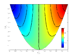
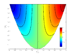
Figure 1: Comparing contour between $M_{2}$ for single frequency (left), $M_{2}$ for gray approximation (center), and $\boldsymbol{B}$-closure (right)

For four sets of moments in typical regions, Figure 2 compares the specific intensity between the $M_{2}$ model and our $\boldsymbol{B}$-closure model. They all qualitatively agree with each other.

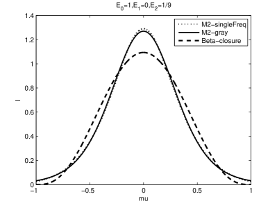
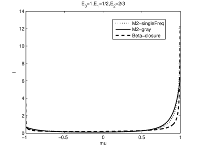
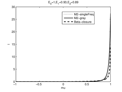
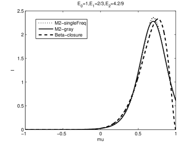
Figure 2: Comparing specific intensity between $M_{2}$ and $\boldsymbol{B}$-closure model

Let us show firstly that the new model based on the $\boldsymbol{B}$-distribution is globally hyperbolic. The Jacobian matrix of the approximate model is

$$\boldsymbol{J}=\left(\begin{array}[]{ccc}0&1&0\\ 0&0&1\\ \dfrac{\partial E_{3}}{\partial E_{0}}&\dfrac{\partial E_{3}}{\partial E_{1}}&\dfrac{\partial E_{3}}{\partial E_{2}}\\ \end{array}\right).$$ (11)

Let $a_{0}=\dfrac{\partial E_{3}}{\partial E_{0}}$, $a_{1}=\dfrac{\partial E_{3}}{\partial E_{1}}$, and $a_{2}=\dfrac{\partial E_{3}}{\partial E_{2}}$, they satisfy

$$\begin{split}a_{0}&=-{\dfrac{E_{{1}}\left(E_{{0}}-E_{{2}}\right)\left(3\,E_{{0}}E_{{2}}-4\,{E_{{1}}}^{2}+{E_{{2}}}^{2}\right)}{\left({E_{{0}}}^{2}+E_{{0}}E_{{2}}-2\,{E_{{1}}}^{2}\right)^{2}}},\\ a_{1}&={\frac{\left(3\,{E_{{0}}}^{2}-E_{{0}}E_{{2}}-2\,{E_{{1}}}^{2}\right)\left(E_{{0}}E_{{2}}-2\,{E_{{1}}}^{2}+{E_{{2}}}^{2}\right)}{\left({E_{{0}}}^{2}+E_{{0}}E_{{2}}-2\,{E_{{1}}}^{2}\right)^{2}}},\\ a_{2}&={\frac{E_{{1}}\left(E_{{0}}-E_{{2}}\right)\left(3\,{E_{{0}}}^{2}+E_{{0}}E_{{2}}-4\,{E_{{1}}}^{2}\right)}{\left({E_{{0}}}^{2}+E_{{0}}E_{{2}}-2\,{E_{{1}}}^{2}\right)^{2}}}.\end{split}$$

The characteristic polynomial of $\boldsymbol{J}$ is

$$p(\lambda)=\lambda^{3}-a_{2}\lambda^{2}-a_{1}\lambda-a_{0}.$$ (12)

We then have the following theorem:

Theorem 3.1 (Global strict hyperbolicity of $\boldsymbol{B}$-closure model).

The $\boldsymbol{B}$-closure model is globally strictly hyperbolic in the interior of the realizable region $\mathcal{M}$, and its propagation speed is less than the speed of light.

Proof.

Let us study it in two cases:

1. For $E_{1}=0$,

   $$p(\lambda)=\lambda\left(\lambda^{2}-\dfrac{E_{2}(3E_{0}-E_{2})}{E_{0}(E_{0}+E_{2})}\right).$$

   Clearly, the three distinct roots of $p(\lambda)$ are $\lambda_{0}=0$ and $\lambda_{\pm}=\pm\sqrt{\dfrac{E_{2}(3E_{0}-E_{2})}{E_{0}(E_{0}+E_{2})}}$. Since $0<\dfrac{E_{2}(3E_{0}-E_{2})}{E_{0}(E_{0}+E_{2})}<1$, all the roots are within $(-1,1)$.

2. Consider $E_{1}\not=0$. Without loss of generality, assume $E_{1}>0$. Then

   $$-1<0<\dfrac{a_{2}}{3}<\dfrac{E_{1}}{E_{0}}<1.$$

   Let $Q=\dfrac{E_{2}}{E_{0}}-\left(\dfrac{E_{1}}{E_{0}}\right)^{2}$, $Z=1-\dfrac{E_{2}}{E_{0}}$, then

   $$p\left(\dfrac{a_{2}}{3}\right)=\dfrac{4}{27}\dfrac{E_{1}}{E_{0}}Q^{2}Zf(Q,Z)>0,$$

   with

   $$f(Q,Z)=\dfrac{68Q^{2}Z^{2}+86QZ^{3}+27Z^{4}+288Q^{3}+360Q^{2}Z+112QZ^{2}}{(2Q+Z)^{6}}.$$

   We notice that

   $$\begin{split}&p(-1)=-\dfrac{(E_{0}-E_{2})^{2}(E_{0}+E_{1})(E_{0}+2E_{1}+E_{2})}{(E_{0}^{2}+E_{0}E_{2}-2E_{1}^{2})^{2}}<0,\\ &p\left(\dfrac{E_{1}}{E_{0}}\right)=-\dfrac{4E_{1}}{E_{0}^{3}}\dfrac{(E_{0}-E_{1})(E_{0}+E_{1})(E_{0}E_{2}-E_{1}^{2})^{2}}{(E_{0}^{2}+E_{0}E_{2}-2E_{1}^{2})^{2}}<0,\\ &p(1)=\dfrac{(E_{0}-E_{2})^{2}(E_{0}-E_{1})(E_{0}-2E_{1}+E_{2})}{(E_{0}^{2}+E_{0}E_{2}-2E_{1}^{2})^{2}}>0,\\ \end{split}$$

   thus $p(\lambda)$ has one root in each intervals $\left(-1,\dfrac{a_{2}}{3}\right)$, $\left(\dfrac{a_{2}}{3},\dfrac{E_{1}}{E_{0}}\right)$, and $\left(\dfrac{E_{1}}{E_{0}},1\right)$. Similar arguments work for $E_{1}<0$.

This ends the proof. ∎

Denote $\lambda_{1}<\lambda_{2}<\lambda_{3}$ to be the three eigenvalues of the Jacobian matrix $\boldsymbol{J}$, then it is clear that the eigenvector corresponding to $\lambda_{j}$ is $\boldsymbol{R}^{(j)}=\left[1~{}~{}\lambda_{j}~{}~{}\lambda_{j}^{2}\right]^{T}$.

Theorem 3.2.

The $\boldsymbol{R}^{(1)}$, $\boldsymbol{R}^{(3)}$-characteristic fields are genuinely non-linear, while the $\boldsymbol{R}^{(2)}$ -characteristic field is neither genuinely non-linear nor linearly degenerate.

Proof.

Let

$$\Delta(\lambda)=\left[1~{}~{}\lambda~{}~{}\lambda^{2}\right]\cdot\dfrac{\partial(a_{0},a_{1},a_{2})}{\partial(E_{0},E_{1},E_{2})}\cdot\left[\begin{array}[]{c}1\\ \lambda\\ \lambda^{2}\\ \end{array}\right].$$

As

$$\nabla\lambda_{j}\cdot\boldsymbol{R}^{(j)}=\left(\left.\dfrac{\mathrm{d}{p}}{\mathrm{d}{\lambda}}\right|_{\lambda=\lambda_{j}}\right)^{-1}\Delta(\lambda),$$

and

$$\left.\dfrac{\mathrm{d}{p}}{\mathrm{d}{\lambda}}\right|_{\lambda=\lambda_{j}}>0,j=1,3;\quad\left.\dfrac{\mathrm{d}{p}}{\mathrm{d}{\lambda}}\right|_{\lambda=\lambda_{2}}<0,$$

$\nabla\lambda_{j}\cdot\boldsymbol{R}^{(j)}=0$ is equivalent to $\lambda_{j}$ being the common root of $\Delta(\lambda)$ and $p(\lambda)$. As the resultant of $p(\lambda)$ and $\Delta(\lambda)$ is

$$\mathrm{res}(p,\Delta,\lambda)=128\,{\frac{E_{{1}}{Q}^{6}{Z}^{4}\left({Z}^{2}+16\,Q+8\,Z\right)\left(Q+Z\right)\left({Z}^{2}+4\,Q\right)^{3}}{E^{4}_{0}\left(2\,Q+Z\right)^{15}}},$$

where $Q=\dfrac{E_{2}}{E_{0}}-\left(\dfrac{E_{1}}{E_{0}}\right)^{2}$, $Z=1-\dfrac{E_{2}}{E_{0}}$. As $Q$ and $Z$ are both positive in the interior of the realizable region $\mathcal{M}$, we have that $\mathrm{res}(p,\Delta,\lambda)\neq 0$ if $E_{1}\neq 0$. Therefore when $E_{1}\neq 0$, all characteristic fields satisfy $\nabla\lambda_{j}\cdot\boldsymbol{R}^{(j)}\neq 0$.

In case that $E_{1}=0$, $\lambda_{2}=0$ is a common root of $p(\lambda)$ and $\Delta(\lambda)$, so

$$\nabla\lambda_{2}\cdot\boldsymbol{R}^{(2)}=0.$$

Meanwhile we have

$$\Delta(\lambda)=2\,{\lambda\left({\lambda}^{2}E_{{0}}-E_{{2}}\right)\frac{\left(3\,E_{{0}}+E_{{2}}\right)\left(E_{{0}}-E_{{2}}\right)}{{E_{{0}}}^{2}\left(E_{{0}}+E_{{2}}\right)^{2}}},$$

thus $\nabla\lambda_{j}\cdot\boldsymbol{R}^{(j)}\not=0$ for $j=1,3$.

Collecting the arguments above, one has that

$$\begin{split}&\nabla\lambda_{j}\cdot\boldsymbol{R}^{(j)}\not=0,\quad\forall(E_{0},E_{1},E_{2})\in\mathcal{M},\quad\text{for}~{}~{}j=1,3;\\ &\mathrm{sign}\left(\nabla\lambda_{j}\cdot\boldsymbol{R}^{(2)}\right)=\mathrm{sign}(E_{1}),\quad\text{under proper scaling of~{}}\boldsymbol{R}^{(2)}.\end{split}$$

∎

We point out that it is also valid for the $M_{2}$ model that $\nabla\lambda_{2}\cdot\boldsymbol{R}^{(2)}=0$ when $E_{1}=0$. Actually, the specific intensity of the $M_{2}$ model is

$$I(\mu)=\dfrac{\alpha_{0}}{(1+\alpha_{1}\mu+\alpha_{2}\mu^{2})^{4}},$$

for the gray case, and

$$I(\mu)=\dfrac{\alpha_{0}}{\exp(1+\alpha_{1}\mu+\alpha_{2}\mu^{2})-1},$$

for the single-frequency case. In this formation, the denominator is always positive on $\mu\in[-1,1]$, and we have that $E_{1}=0$ implies $\alpha_{1}=0$. Therefore,

$$E_{3}=0,~{}~{}\lambda_{2}=0,\quad\forall~{}(E_{0},0,E_{2})\in\mathcal{M}.$$

Direct calculations show $\nabla\lambda_{2}\cdot\boldsymbol{R}^{(2)}\left|{}_{(E_{0},0,E_{2})}\right.=\dfrac{\partial a_{0}}{\partial E_{0}}\left|{}_{(E_{0},0,E_{2})}\right.=0$.

Let us summarize briefly some advantages of the new model:

1. The ansatz for the specific intensity preserves positivity and has explicit closure relationship;

2. The model derived is conservative and globally hyperbolic;

3. The signal speed of the new model is less than the speed of light;

4. The closure is very close to that of $M_{2}$;

We present some numerical results for some benchmark problems to show the quality of the new model as an approximation of the $M_{2}$ model.

4 Numerical Results

Our approximate $M_{2}$ model of (9) is therefore

$$\dfrac{1}{c}\dfrac{\partial E_{0}}{\partial t}+\dfrac{\partial E_{1}}{\partial z}=-\sigma_{a}E_{0},$$ (13)

$$\dfrac{1}{c}\dfrac{\partial E_{1}}{\partial t}+\dfrac{\partial E_{2}}{\partial z}=-\left[\sigma_{a}+\sigma_{s}\right]E_{1},$$

$$\dfrac{1}{c}\dfrac{\partial E_{2}}{\partial t}+\dfrac{\partial E_{3}}{\partial z}=-\sigma_{a}E_{2}+\sigma_{s}\left(\dfrac{E_{0}}{3}-E_{2}\right).$$

We consider the angular closure for a single frequency $\nu=1$. We solve equation (13) using the canonical finite volume scheme with the Lax-Friedrich numerical flux, and the source term is treated implicitly.

To impose an inflow boundary condition, we only need to impose the value of the flux on the boundary. We derive it using upwind on the kinetic scale. As we know the moments on the left and right cells, we can reconstruct $\hat{I}(E^{l}_{0},E^{l}_{1},E^{l}_{2},\mu)$ and $\hat{I}(E^{r}_{0},E^{r}_{1},E^{r}_{2},\mu)$ on the left and right cells using the ansatz (10), then integrate over $\mu$ to have

$$E_{j}=\int_{0}^{1}\mu^{j}\hat{I}(\mu,E^{l}_{0},E^{l}_{1},E^{l}_{2})\,{\rm d}\mu+\int_{-1}^{0}\mu^{j}\hat{I}(\mu,E^{r}_{0},E^{r}_{1},E^{r}_{2})\,{\rm d}\mu,\quad\text{for}~{}~{}j=1,2,3,$$

to give the flux on the boundary.

We compare our model to numerical solutions of the true $M_{2}$ model, which for the single-frequency case uses the ansatz (6). We compute $M_{2}$ solutions using the kinetic scheme and optimization techniques given in [2]. The entropy from that work is replaced with the Bose-Einstein entropy (5), and to avoid the singularity in the ansatz (6) when the polynomial $\boldsymbol{\alpha}\cdot\boldsymbol{m}$ passes through zero, we limit the step-size in the Armijo line search so that the polynomial $\boldsymbol{\alpha}\cdot\boldsymbol{m}$ remains negative at every angular quadrature point. Our solutions are computed with 1000 cells, and we note that none of the computations below required the use of the isotropic regularization technique.

Below we give the numerical results for three examples.

Example 4.1 (Two-beam).

The absorption coefficient is $\sigma_{a}=2$, the scattering coefficient $\sigma_{s}=0$, and the speed of light is taken to be $c=1$. The spatial domain is $z\in[0,1]$. The initial value is set as $E_{0}=10^{-7}$, $E_{1}=0$, $E_{2}=\dfrac{1}{3}E_{0}$ for all $z$. Inflow boundary condition are imposed on both ends, thus the specific intensity on the boundaries are $I(t,0,\mu)=\exp(-10(\mu-1)^{2})$ on the left boundary $z=0$, and $I(t,1,\mu)=\exp(-10(\mu+1)^{2})$ on the right boundary $z=1$.

In Figure 3 we compares the steady-state solution of $E_{0}$ between the $M_{2}$ model and the $\boldsymbol{B}$-closure model.

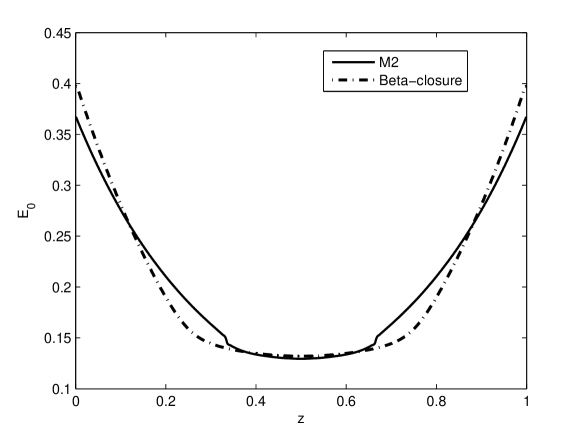
Figure 3: steady state solution for two-beam problem

Example 4.2 (Isotropic inflow into vacuum).

In this example, we consider the spatial domain $z\in[-\infty,1]$ with an isotropic inflow source is imposed on the right boundary into a domain which is unbounded on the left. We take $\sigma_{a}=\sigma_{s}=0$. Initially, for all $z$ , we take $E_{0}=10^{-8}$, $E_{1}=0$, $E_{2}=\dfrac{1}{3}E_{0}$. The isotropic inflow is specified at $z=1$. The specific intensity outside the right boundary is $I(\mu)=0.5$. We carry out the computation from $t_{0}=0$ to $t=0.5418$ and $0.8$.

The results are in Figure 4, which are the value of $E_{0}$ at $t=0.5418$ and $t=0.8$ for both the $\boldsymbol{B}$-closure model and the $M_{2}$ model.

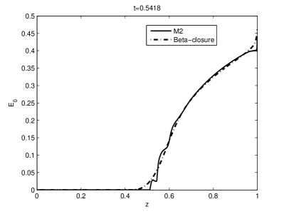
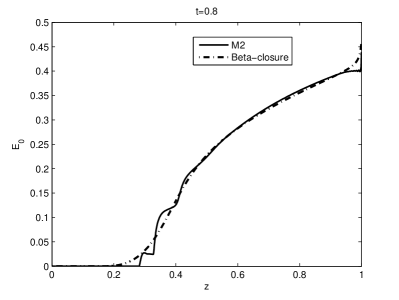
Figure 4: Results for inflow into vacumm problem

Example 4.3 (Plane source).

In this test the spatial domain is unbounded, and the initial value is taken as $E_{0}(z)=\delta(z)+10^{-8}$, $E_{1}=0$ and $E_{2}=\dfrac{1}{3}E_{0}$. The simulation time interval is from $t_{0}=0$ to $t=0.7005$ and $t=0.9043$.

The numerical results of $E_{0}$ for $M_{2}$ and the $\boldsymbol{B}$-closure model are in Figure 5.

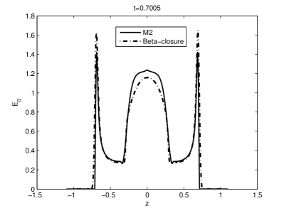
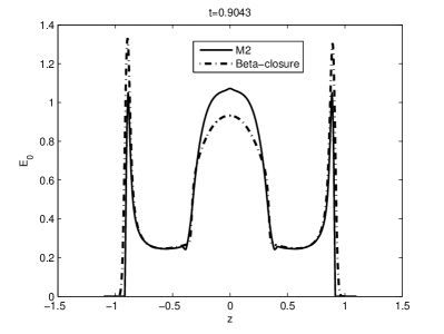
Figure 5: Results for plane source problem

5 Conclusion

An approximate $M_{2}$ model for the radiative transfer slab geometry in the cases of single-frequency and grey medium is proposed. The new model is based on an ansatz formulated as a $\boldsymbol{B}$-distribution. It shares most of the advantages of the $M_{2}$ model while it has an explicit closure. We are now working the extension of this idea to a three dimensional configuration and a many moment model.

References

- [1] Thomas A Brunner and James Paul Holloway. One-dimensional riemann solvers and the maximum entropy closure. Journal of Quantitative Spectroscopy and Radiative Transfer, 69(5):543–566, 2001.
- [2] Graham W Alldredge, Cory D Hauck, Dianne P OʼLeary, and André L Tits. Adaptive change of basis in entropy-based moment closures for linear kinetic equations. Journal of Computational Physics, 258:489–508, 2014.
- [3] Graham W Alldredge, Cory D Hauck, and André L Tits. High-order entropy-based closures for linear transport in slab geometry ii: A computational study of the optimization problem. SIAM Journal on Scientific Computing, 34(4):B361–B391, 2012.
- [4] Christophe Berthon, Pierre Charrier, and Bruno Dubroca. An hllc scheme to solve the model of radiative transfer in two space dimensions. Journal of Scientific Computing, 31(3):347–389, 2007.
- [5] R. Curto and L. Fialkow. Recursiveness, positivity and truncated moment problems. Houston J. Math, 17(4):603–635, 1991.
- [6] Bruno Dubroca and J-L Feugeas. Theoretical and numerical study on a moment closure hierarchy for the radiative transfer equation. Comptes Rendus de l’Academie des Sciences Series I Mathematics, 329(10):915–920, 1999.
- [7] C Kristopher Garrett and Cory D Hauck. A comparison of moment closures for linear kinetic transport equations: The line source benchmark. Transport Theory and Statistical Physics, 42(6-7):203–235, 2013.
- [8] Harold Grad. On the kinetic theory of rarefied gases. Communications on pure and applied mathematics, 2(4):331–407, 1949.
- [9] C David Levermore. Moment closure hierarchies for kinetic theories. Journal of Statistical Physics, 83(5-6):1021–1065, 1996.
- [10] Ryan G McClarren, James Paul Holloway, and Thomas A Brunner. On solutions to the equations for thermal radiative transfer. Journal of Computational Physics, 227(5):2864–2885, 2008.
- [11] Gerald N Minerbo. Maximum entropy eddington factors. Journal of Quantitative Spectroscopy and Radiative Transfer, 20(6):541–545, 1978.
- [12] Philipp Monreal and Martin Frank. Higher order minimum entropy approximations in radiative transfer. arXiv preprint arXiv:0812.3063, 2008.
- [13] Edgar Olbrant, Cory D Hauck, and Martin Frank. A realizability-preserving discontinuous galerkin method for the m1 model of radiative transfer. Journal of Computational Physics, 231(17):5612–5639, 2012.
- [14] Eleuterio F Toro. Riemann solvers and numerical methods for fluid dynamics: a practical introduction. Springer Science & Business Media, 2009.
- [15] V Vikas, CD Hauck, ZJ Wang, and Rodney O Fox. Radiation transport modeling using extended quadrature method of moments. Journal of Computational Physics, 246:221–241, 2013.