SLRMA: Sparse Low-Rank Matrix Approximation for Data Compression

Abstract

Low-rank matrix approximation (LRMA) is a powerful technique for signal processing and pattern analysis. However, its potential for data compression has not yet been fully investigated in the literature. In this paper, we propose sparse low-rank matrix approximation (SLRMA), an effective computational tool for data compression. SLRMA extends the conventional LRMA by exploring both the intra- and inter-coherence of data samples simultaneously. With the aid of prescribed orthogonal transforms (e.g., discrete cosine/wavelet transform and graph transform), SLRMA decomposes a matrix into a product of two smaller matrices, where one matrix is made of extremely sparse and orthogonal column vectors, and the other consists of the transform coefficients. Technically, we formulate SLRMA as a constrained optimization problem, i.e., minimizing the approximation error in the least-squares sense regularized by $\ell_{0}$-norm and orthogonality, and solve it using the inexact augmented Lagrangian multiplier method. Through extensive tests on real-world data, such as 2D image sets and 3D dynamic meshes, we observe that (i) SLRMA empirically converges well; (ii) SLRMA can produce approximation error comparable to LRMA but in a much sparse form; (iii) SLRMA-based compression schemes significantly outperform the state-of-the-art in terms of rate-distortion performance.

I Introduction

Given a matrix $\mathbf{X}\in\mathbb{R}^{m\times n}$ corresponding to $n$ data samples in $\mathbb{R}^{m}$, low-rank matrix approximation (LRMA) (a.k.a. principal component analysis (PCA) and subspace factorization) seeks a matrix $\widehat{\mathbf{X}}\in\mathbb{R}^{m\times n}$ of rank $k\ll\min(m,n)$ that best approximates $\mathbf{X}$ in the least-squares sense [1]. Alternatively, the rank constraint can be implicitly expressed in a factored form, i.e., $\mathbf{X}\approx\widehat{\mathbf{X}}=\mathbf{B}\mathbf{C}$ where $\mathbf{B}\in\mathbb{R}^{m\times k}$ and $\mathbf{C}\in\mathbb{R}^{k\times n}$ (see Figure 1). This decomposition is not unique, since $(\mathbf{BA})(\mathbf{A}^{-1}\mathbf{C})=\mathbf{BC}$ holds for any invertible matrix $\mathbf{A}\in\mathbb{R}^{k\times k}$. To reduce the solution space, one often requires the decomposed matrix $\mathbf{B}$ to be column-orthogonal.

Since LRMA is able to reveal the inherent structure of the input data, it has been applied to a wide spectrum of engineering applications, including data compression [2], [3], background subtraction [4], [5], classification and clustering [6], [7], image/video restoration and denoising [8], [9], image alignment and interpolation [10], [11], structure from motion [12], [13], [14], etc. We refer the readers to the survey paper [15] for more details.

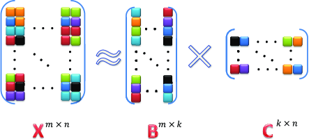
Figure 1: Illustration of low-rank matrix approximation. $k\ll\min(m,n)$ and $\mathbf{B}^{\textsf{T}}\mathbf{B}=\mathbf{I}_{k}$; Each column of $\mathbf{X}$ corresponds to one data sample.

Among the above-mentioned applications, we are particularly interested in data compression. At the first glance, applying LRMA to data compression seems to be straightforward, since one only needs to store $k(m+n)$ elements, with small approximation error introduced in LRMA. Such an idea has been used extensively to compress various types of data, e.g., images/videos [2, 16, 17, 18, 19, 20, 3], 3D motion data [21, 22, 23, 24, 25], traffic data [26, 27, 28]. However, data samples usually exhibit both intra-coherence (i.e., coherence within each data sample) and inter-coherence (i.e., coherence among different data samples). LRMA can exploit the inter-coherence well, i.e., using $\mathbf{B}$ with much smaller orthogonal columns to represent $\mathbf{X}$, but it fails to address the intra-coherence in the columns of $\bf B$, and hereby compromises the compression performance [21], [22], [25], [26], [27], [28]. Figure 2(a) shows the problem using a 2D image set. One can clearly see that the columns of $\mathbf{B}$ produced by LRMA are locally smooth (the bright areas), indicating the strong coherence.

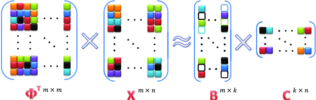
Figure 3: Illustration of sparse LRMA. ${\bf\Phi}$ is a prescribed orthogonal transform, such as DCT, DWT and GT, where each column corresponds to a frequency. The column vectors in matrix $\mathbf{B}$ are sparse and orthogonal, i.e., $\mathbf{B}^{\textsf{T}}\mathbf{B}=\mathbf{I}_{k}$. The empty boxes in $\mathbf{B}$ are zeros.

In this paper, we propose sparse low-rank matrix approximation (SLRMA) for data compression. In contrast to the existing methods, which usually explore intra- and inter-coherence separately (see Section II), SLRMA is able to explore both the intra- and inter-coherence of data samples simultaneously from the perspective of optimization and transform. As Figure 3 shows, SLRMA multiplies a prescribed orthogonal matrix $\mathbf{\Phi}\in\mathbb{R}^{m\times m}$ (such as discrete consine/wavelet transform (DCT/DWT) and graph transform) to the input matrix $\bf X$ and then factors $\mathbf{\Phi}^{\textsf{T}}\mathbf{X}$ into a product of the extremely sparse and column-orthogonal matrix $\mathbf{B}$ and the coefficient matrix $\mathbf{C}$. We formulate SLRMA as a constrained optimization problem, i.e., minimizing the approximation error in least-squares sense under the $\ell_{0}$-norm and orthogonality constraints, and solve it using the inexact augmented Lagrangian multiplier method.

Through extensive tests on real-world data, such as 2D image sets and 3D dynamic meshes, we observe that (i) SLRMA empirically converges well; (ii) SLRMA can produce comparable approximation error as LRMA but in a much sparser form; (iii) SLRMA-based compression schemes outperform the state-of-the-art scheme to a large extent in terms of rate-distortion performance. Figure 2(b) visualizes the column vectors of $\mathbf{B}$ of the proposed SLRMA which produces the same approximation error as that of LRMA in Figure 2(a), where one can clearly see that column vectors of SLRMA do not exhibit such intra-coherence.

1^st2^nd3^rd4^th5^th 1^st2^nd3^rd4^th5^th 1^st2^nd3^rd4^th5^th

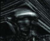
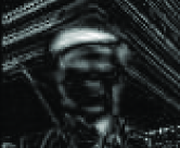
(a) Column vectors of $\mathbf{B}$ in LRMA

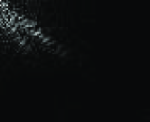
(b) Column vectors of $\mathbf{B}$ in SLRMA

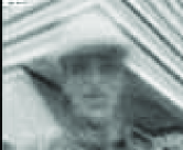
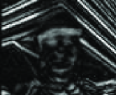
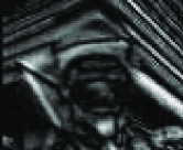
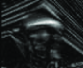
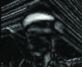
(c) Column vectors of $\breve{\mathbf{B}}$ in Equation (9).

Figure 2: Comparison of LRMA and SLRMA in terms of intra-correlation in $\bf B$. The test image set contains 150 frames of the “foreman” video of resolution $88\times 72$, representing in a matrix $\mathbf{X}\in\mathbb{R}^{6336\times 150}$. Some samples are shown in Figure 5(a). We visualize the first five column vectors of $\mathbf{B}$ for LRMA and SLRMA in (a) and (b). Both LRMA and SLRMA approximate matrix $\mathbf{X}$ with the same approximation error. In SLRMA, we set $\bf\Phi$ the 2D DCT matrix.

The rest of this paper is organized as follows: Section II reviews the related work on LRMA-based data compression. Section III briefly introduces LRMA and graph transform. Sections IV presents the sparse LRMA algorithm followed by experimental results in Section V. Finally, Section VI concludes this paper and points out several promising future directions.

Notations. Throughout this paper, scalars are denoted by italic lower-case letters, vectors by bold lower-case letters and matrices by upper-case ones, respectively. For instance, we consider a matrix $\mathbf{A}\in\mathbb{R}^{m\times n}$. The $i$-th row and $j$-th column of $\bf A$ are represented by $\mathbf{a}^{i}\in\mathbb{R}^{1\times n}$ and $\mathbf{a}_{j}\in\mathbb{R}^{m\times 1}$, respectively. Let $a_{ij}$ be the $(i,j)$-th entry of $\mathbf{A}$ with its absolute being $|a_{ij}|$. $\mathbf{A}^{\textsf{T}}$ and $\mathbf{A}^{\dagger}$ are the transpose and pseudoinverse of $\mathbf{A}$. We denote by $\|\mathbf{A}\|_{F}=\sqrt{\sum_{i=1}^{m}\sum_{j=1}^{n}a_{ij}^{2}}$ and $\|\mathbf{A}\|_{\infty}=\max_{i,j}{|a_{ij}|}$ the Frobenious norm and the $\ell_{\infty}$ norm of $\mathbf{A}$, respectively. The $\ell_{0}$-norm $\|\mathbf{A}\|_{0}$ counts the number of nonzero entries in $\mathbf{A}$. Let ${\rm Tr}(\mathbf{A})=\sum_{i}a_{ii}$ be the trace of $\bf A$. $\mathbf{I}_{k}$ is the identity matrix of size $k\times k$.

II Related Work

In this section, we briefly review the LRMA-based methods for data compression. Yang and Lu [16] represented the basis vectors using vector quantization for image coding. Similar techniques were also adopted in video compression [2], [17]. Note that training coodbooks is computationally expensive due to the large amount of training data. Moreover, the trained codebooks may be biased, leading to large approximation error to the data if they are fundamentally different than the training data. Du et al. [18] applied LRMA to hyperspectral images to remove the spectral coherence, then adopted JP2K [29], the standard image encoder, to further compress the basis vectors. Hou et al. [3] extracted a few keyframes from geometry videos and compressed them using a standard video encoder H.264/AVC [30], and the whole geometry video was reconstructed by linearly interpolating the decompressed keyframes. Chen et al. [19] and Hou et al. [20] also presented robust LRMA [4] and video encoders combined compression frameworks for surveillance videos and geometry videos, respectively.

3D triangle meshes are a simple and flexible tool to represent complex 3D objects for graphics applications ranging from modeling, animation to rendering. A mesh consists of structural and geometric data. Dynamic meshes are the sequence of triangle meshes with the same connectivity, representing a deformable model with time-varying geometry. Alex and Müller [21] adopted LRMA to compress 3D dynamic meshes, representing each frame as the linear combination of few basis vectors. Karni and Gostamn [22] improved this scheme by applying second-order linear predictive coding to coefficients to further remove the temporal coherence. Heu et al. [31] proposed an adaptive bit plane coder to encode the basis vectors to achieve progressive transmission. However, these methods cannot eliminate the spatial (or intra-) coherence. Unlike [21, 22, 31], trajectory-LRMA was employed in [23, 24, 32, 33, 34], which represents trajectories of vertices as a linear combination of few basis vectors. Sattler et al. [32] proposed clustered LRMA to compress 3D dynamic meshes, in which clustering of trajectories and trajectory-LRMA were performed simultaneously to explore the spatial and temporal correlation. Vásǎ et al.  [34] studied the trajectory-LRMA-based compression for 3D dynamic meshes systematically. For example, to remove the coherence among basis vectors, they proposed predictive coding to encode them. They also introduced three types of predictions to exploit the coherence among coefficients, namely parallelogram-based prediction [33], least squares prediction, and radial basis function-based prediction [23]. Recently, they used the discrete geometric Laplacian of a computed average surface to encode the coefficients [24], and achieved the state-of-the-art rate-distortion performance. But this method requires the models of sequences to be manifolds due to the process of computing an average surface, limiting its range of applications.

III Preliminaries

III-A Low-Rank Matrix Approximation

Given $\mathbf{X}\in\mathbb{R}^{m\times n}$, the LRMA problem can be mathematically formulated as

$$\min_{\mathbf{B}\in\mathbb{R}^{m\times k}\atop\mathbf{C}\in\mathbb{R}^{k\times n}}\|\mathbf{X}-\mathbf{B}\mathbf{C}\|_{F}^{2}$$

$$\mathrm{subject}~{}\mathrm{to}~{}~{}\mathbf{B}^{\textsf{T}}\mathbf{B}=\mathbf{I}_{k}.$$ (1)

Setting the derivative of the objective function of $\bf C$ to zero, we obtain $\mathbf{C}=\mathbf{B}^{\textsf{T}}\mathbf{X}$. Since $\|\mathbf{A}\|_{F}^{2}={\rm Tr}(\mathbf{A}\mathbf{A}^{\textsf{T}})$ and ${\rm Tr}(\mathbf{A})={\rm Tr}(\mathbf{A}^{\textsf{T}})$, we can expand the objective function as

$$\|\mathbf{X}-\mathbf{B}\mathbf{C}\|_{F}^{2}$$

$$={\rm Tr}\left\{(\mathbf{X}-\mathbf{B}\mathbf{C})(\mathbf{X}-\mathbf{B}\mathbf{C})^{\textsf{T}}\right\}$$

$$={\rm Tr}\left(\mathbf{X}\mathbf{X}^{\textsf{T}}\right)-2{\rm Tr}\left(\mathbf{B}\mathbf{C}\mathbf{X}^{\textsf{T}}\right)+{\rm Tr}\left(\mathbf{B}\mathbf{C}\mathbf{C}^{\textsf{T}}\mathbf{B}^{\textsf{T}}\right).$$ (2)

Substituting $\mathbf{C}=\mathbf{B}^{\textsf{T}}\mathbf{X}$ into (2) and dropping the constant term, we obtain the equivalent problem of (1), i.e.,

$$\max_{\mathbf{B}}{\rm Tr}\left(\mathbf{B}^{\textsf{T}}\mathbf{X}\mathbf{X}^{\textsf{T}}\mathbf{B}\right)$$

$$\mathrm{subject}~{}\mathrm{to}~{}~{}\mathbf{B}^{\textsf{T}}\mathbf{B}=\mathbf{I}_{k}.$$ (3)

It is well known that the problem in (3) has an optimal solution [35], which consists of $k$ eigenvectors of $\mathbf{X}\mathbf{X}^{\textsf{T}}$, corresponding to the $k$ largest eigenvalues. We refer the readers to  [36] for more technical details about LRMA.

III-B Graph Transform

Let $\mathbf{s}\in\mathbb{R}^{n\times 1}$ be a signal defined on an undirected, connected and unweighted graph with $n$ vertices denoted by $\mathcal{G}=(\mathcal{V},\mathcal{E})$, where $\mathcal{V}$ and $\mathcal{E}$ are the sets of vertices and edges, respectively. The graph’s adjacency matrix $\mathbf{E}\in\mathbb{R}^{n\times n}$ is given by

$$e_{ij}=\left\{\begin{array}[]{cc}1&{\rm if}~{}(i,j)\in\mathcal{E}\\ 0&{\rm otherwise},\end{array}\right.$$ (4)

and its degree matrix $\mathbf{F}\in\mathbb{R}^{n\times n}$, a diagonal matrix, is defined as

$$f_{ij}=\left\{\begin{array}[]{cc}\sum_{l=1}^{n}e_{il}&{\rm if}~{}i=j\\ 0&{\rm otherwise.}\end{array}\right.$$ (5)

Then the graph Laplacian matrix $\mathbf{L}\in\mathbb{R}^{n\times n}$ is computed as

$$\centering\mathbf{L}=\mathbf{F}-\mathbf{E}.\@add@centering$$ (6)

Since $\mathbf{L}$ is a real symmetric matrix, it has a set of real and non-negative eigenvalues denoted by $\{\lambda_{i}\}_{i=1,2,\cdots,n}$ associated with a complete set of orthogonal eigenvectors denoted by $\{\mathbf{u}_{i}\in\mathbb{R}^{n\times 1}\}_{i=1,2,\cdots,n}$, i.e.,

$$\mathbf{L}=\mathbf{U}_{gt}{\bf\Lambda}\mathbf{U}_{gt}^{\textsf{T}},$$ (7)

where $\mathbf{U}_{gt}=[\mathbf{u}_{1}~{}\mathbf{u}_{2}~{}\cdots~{}\mathbf{u}_{n}]\in\mathbb{R}^{n\times n}$ and ${\bf\Lambda}={\rm diag}(\lambda_{1},\cdots,\lambda_{n})\in\mathbb{R}^{n\times n}$.

Similar to the Fourier bases, which are the eigenvectors of the one-dimensional Laplace operator, the eigenvectors of $\mathbf{L}$ also possess harmonic behavior [37]. Following [38], we call the eigenvector matrix based transformation graph transform (GT). Thus, one can decorrelate the signal as follows:

$$\centering\mathbf{r}=\mathbf{U}_{gt}^{\textsf{T}}\mathbf{s},\@add@centering$$ (8)

where $\mathbf{r}\in\mathbb{R}^{n\times 1}$ consists of sparse or approximately sparse transform coefficients.

IV Sparse Low-Rank Matrix Approximation

IV-A Problem Statement

Recall that LRMA can effectively exploit the inter-coherence of data samples, but it fails to exploit their intra-coherence. Thus, the intra-coherence is delivered into the columns of $\mathbf{B}$. The issue to be addressed is how to effectively exploit such intra-coherence.

It is well-known that some prescribed orthogonal transforms, e.g, DCT, DWT, and GT denoted as ${\bf\Phi}\in\mathbb{R}^{m\times m}$ (${\bf\Phi}^{\textsf{T}}{\bf\Phi}={\bf\Phi}{\bf\Phi}^{\textsf{T}}=\mathbf{I}_{m}$), can decorrelate signals [37], [39], i.e., producing approximately sparse transform coefficients. In order to explore the intra-coherence inheriting from the data samples, one may consider applying $\bf\Phi$ to columns of $\mathbf{B}$ following LRMA, which is similar to techniques in [18] and [3], but such stepwise manner induces large reconstruction error (See results in Section V). The reasons are: (i) LRMA suppresses the spatial characteristics of data, so they cannot explore the intra-coherence very well in a direct way; (ii) columns of $\mathbf{B}$ are separately decorrelated, which cannot preserve the relationship among them (e.g., orthogonality). Therefore, we propose SLRMA to explore the intra- and inter- coherence simultaneously and integrally, and it is cast as the following optimization problem:

$$\min_{\breve{\mathbf{B}},\mathbf{C}}\left\|\mathbf{X}-\breve{\mathbf{B}}\mathbf{C}\right\|_{F}^{2}$$

$${\rm subject~{}to~{}~{}}\breve{\mathbf{B}}^{\textsf{T}}\breve{\mathbf{B}}=\mathbf{I}_{k}$$

$$~{}~{}~{}~{}~{}\sum_{i=1}^{k}\left\|{\bf\Phi}^{\textsf{T}}\breve{\mathbf{b}}_{i}\right\|_{0}=\left\|{\bf\Phi}^{\textsf{T}}\breve{\mathbf{B}}\right\|_{0}\leq s.$$ (9)

Note that we constrain $\breve{\mathbf{B}}$ to be sparse with respect to $\bf\Phi$, making the derived $\breve{\mathbf{B}}$ via optimization adapted to $\bf\Phi$. The difference between $\breve{\mathbf{B}}$ and $\mathbf{B}$ by LRMA can be observed by comparing Figure 2(a) and Figure 2(c). Furthermore, taking $\|{\bf\Phi}^{\textsf{T}}\mathbf{A}\|_{F}^{2}=\|\mathbf{A}\|_{F}^{2}$ and with a slight abuse of notation (i.e, replacing ${\bf\Phi}^{\textsf{T}}\breve{\mathbf{B}}$ by $\mathbf{B}$), we can rewrite the problem in (9) as

$$\min_{\mathbf{B},\mathbf{C}}~{}\|{\bf\Phi}^{\textsf{T}}\mathbf{X}-\mathbf{B}\mathbf{C}\|_{F}^{2}$$

$${\rm subject~{}to}~{}~{}\mathbf{B}^{\textsf{T}}\mathbf{B}=\mathbf{I}_{k}~{}~{}{\rm and}~{}~{}\|\mathbf{B}\|_{0}\leq s.$$ (10)

In all, the proposed SLRMA can be interpreted as follows: the transform coefficients of data samples are low-rank approximated under the sparsity constraint, in which $\bf\Phi$ and the sparsity constraint can explore the intra-coherence integrally, and the low-rank representation can explore the inter-coherence. These two types of decorrelation are simultaneously performed through optimization. Regarding $\bf\Phi$, it can be set according to data samples. For example, we can adopt DCT or DWT as the transform matrix for natural images, and the GT matrix for data defined on general graphs.

IV-B Numerical Solver

Similar to the process of (1) to (3), the problem in (10) can be simplified as

$$\min_{\mathbf{B}}-\|\mathbf{Z}^{\textsf{T}}\mathbf{B}\|_{F}^{2}$$

$${\rm subject~{}to}~{}~{}\mathbf{B}^{\textsf{T}}\mathbf{B}=\mathbf{I}_{k}~{}~{}{\rm and}~{}~{}\|\mathbf{B}\|_{0}\leq s,$$ (11)

where $\mathbf{Z}={\bf\Phi}^{\textsf{T}}\mathbf{X}$. Instead of solving (11) directly, we solve its Lagrangian version:

$$\min_{\mathbf{B}}~{}-\|\mathbf{Z}^{\textsf{T}}\mathbf{B}\|_{F}^{2}+\gamma\|\mathbf{B}\|_{0}$$

$${\rm subject~{}to}~{}~{}\mathbf{B}^{\textsf{T}}\mathbf{B}=\mathbf{I}_{k},$$ (12)

where the regularization parameter $\gamma$ controls the sparsity of $\mathbf{B}$: the larger the value of $\gamma$ is, the sparser the matrix $\mathbf{B}$ is.

We adopt the inexact augmented Lagrangian multiplier method (IALM) [40] to solve (12). Introducing two auxiliary matrices $\mathbf{P}\in\mathbb{R}^{m\times k}$ and $\mathbf{Q}\in\mathbb{R}^{m\times k}$, we rewrite (12) equivalently as

$$\min_{\mathbf{B},\mathbf{P},\mathbf{Q}}~{}-\|\mathbf{Z}^{\textsf{T}}\mathbf{B}\|_{F}^{2}+\gamma\|\mathbf{P}\|_{0}$$

$${\rm subject~{}to}~{}~{}\mathbf{P}=\mathbf{B},~{}~{}\mathbf{Q}=\mathbf{B},~{}~{}\mathbf{Q}^{\textsf{T}}\mathbf{Q}=\mathbf{I}_{k}.$$ (13)

The augmented Lagrangian form of (13) is given by

$$\operatorname*{arg\,min}_{\mathbf{B},\mathbf{P},\atop\mathbf{Q}^{\textsf{T}}\mathbf{Q}=\mathbf{I}_{k}}-\|\mathbf{Z}^{\textsf{T}}\mathbf{B}\|_{F}^{2}+\gamma\|\mathbf{P}\|_{0}+{\rm Tr}\left(\mathbf{Y}_{P}^{\textsf{T}}(\mathbf{B}-\mathbf{P})\right)$$

$$~{}+{\rm Tr}\left(\mathbf{Y}_{Q}^{\textsf{T}}(\mathbf{B}-\mathbf{Q})\right)+\frac{\rho}{2}\left(\|\mathbf{B}-\mathbf{P}\|_{F}^{2}+\|\mathbf{B}-\mathbf{Q}\|_{F}^{2}\right),$$ (14)

where $\mathbf{Y}_{p}$ and $\mathbf{Y}_{q}\in\mathbb{R}^{m\times k}$ are the Lagrange multipliers, and the regularization parameter $\rho$ is a positive scalar.

With initialized $\bf P$, $\bf Q$, $\mathbf{Y}_{P}$, and $\mathbf{Y}_{Q}$, the IALM solves the optimization problem (14) in an iterative manner (see Algorithm 1 for the pseudocode). Each iteration alternatively solves the following four subproblems:

1) The $\mathbf{B}$-Subproblem: The $\bf B$-subproblem is with a quadratic form:

$$\min_{\mathbf{B}}~{} -\|\mathbf{Z}^{\textsf{T}}\mathbf{B}\|_{F}^{2}+\frac{\rho}{2}\Big{(}\|\mathbf{B}-\mathbf{P}+\mathbf{Y}_{P}/\rho\|_{F}^{2}$$

$$+\|\mathbf{B}-\mathbf{Q}+\mathbf{Y}_{Q}/\rho\|_{F}^{2}\Big{)}.$$ (15)

Equation (15) reaches the minimal when the first-order derivative to $\bf B$ vanishes:

$$\centering\mathbf{B}=\left(2\rho\mathbf{I}_{m}-2\mathbf{Z}\mathbf{Z}^{\textsf{T}}\right)^{-1}\Big{(}\rho(\mathbf{P}+\mathbf{Q})-\mathbf{Y}_{P}-\mathbf{Y}_{Q}\Big{)}.\@add@centering$$ (16)

2) The $\mathbf{P}$-Subproblem: The $\mathbf{P}$-subproblem is written as

$$\centering\min_{\mathbf{P}}\gamma\|\mathbf{P}\|_{0}+\frac{\rho}{2}\|\mathbf{P}-(\mathbf{B}+\mathbf{Y}_{P}/\rho)\|_{F}^{2}.\@add@centering$$ (17)

Let $\widetilde{\mathbf{B}}=\mathbf{B}+\mathbf{Y}_{P}/\rho$, and Equation (17) can be rewritten in element-wise as

$$\centering\min_{\{p_{ij}\}}\sum_{i,j}\gamma\mathbf{1}_{(p_{ij}\neq 0)}+\frac{\rho}{2}\left(p_{ij}-\widetilde{b}_{ij}\right)^{2},\@add@centering$$ (18)

where $\mathbf{1}_{(p_{ij}\neq 0)}$ is a indicator function, i.e., $\mathbf{1}_{(p_{ij}\neq 0)}=1$, if $p_{ij}\neq 0$ and 0 otherwise. Furthermore, the objective function (18) is minimized if each independent univariate in the summarization is minimized, i.e.,

$$\centering\min_{p_{ij}}\gamma\mathbf{1}_{(p_{ij}\neq 0)}+\frac{\rho}{2}\left(p_{ij}-\widetilde{b}_{ij}\right)^{2}.\@add@centering$$ (19)

It can be easily checked that $p_{ij}$ has an unique solution given by the hard thresholding operator, i.e.,

$$p_{ij}=\left\{\begin{array}[]{cc}\widetilde{b}_{ij}&{\rm if}~{}|\widetilde{b}_{ij}|>\sqrt{2\gamma/\rho}\\ 0&{\rm otherwise}.\end{array}\right.$$ (20)

3) The $\mathbf{Q}$-Subproblem: It is expressed as

$$\centering\min_{\mathbf{Q}^{\textsf{T}}\mathbf{Q}=\mathbf{I}_{k}}\frac{\rho}{2}\|\mathbf{Q}-(\mathbf{B}+\mathbf{Y}_{Q}/\rho)\|_{F}^{2}.\@add@centering$$ (21)

According to Theorem 1, the problem (21) has a closed-form solution:

$$\centering\mathbf{Q}=\widehat{\mathbf{B}}\mathbf{V}\mathbf{D}^{-1/2}\mathbf{V}^{\textsf{T}},\@add@centering$$ (22)

where $\mathbf{\widehat{B}}=\mathbf{B}+\mathbf{Y}_{Q}/\rho$, and the orthogonal matrix $\mathbf{V}\in\mathbb{R}^{k\times k}$ and the diagonal matrix $\mathbf{D}\in\mathbb{R}^{k\times k}$ satisfy the eigendecomposition of $\widehat{\mathbf{B}}^{\textsf{T}}\widehat{\mathbf{B}}$, i.e., $\widehat{\mathbf{B}}^{\textsf{T}}\widehat{\mathbf{B}}=\mathbf{V}\mathbf{D}\mathbf{V}^{\textsf{T}}$.

Theorem 1 ([41])

Given $\mathbf{X}\in\mathbb{R}^{m\times n}$ and ${\rm rank}(\mathbf{X})=n$, the constrained quadratic problem:

$$\centering\mathbf{X}^{*}=\operatorname*{arg\,min}_{\mathbf{X}\in\mathbb{R}^{m\times n}}\frac{1}{2}\|\mathbf{X}-\mathbf{A}\|_{F}^{2},~{}~{}{\rm subject~{}to}~{}\mathbf{X}^{\textsf{T}}\mathbf{X}=\mathbf{I}_{n}\@add@centering$$

has the closed-form solution, i.e.,$\mathbf{X}^{*}=\mathbf{A}\widetilde{\mathbf{V}}\widetilde{\mathbf{D}}^{-1/2}\widetilde{\mathbf{V}}^{\textsf{T}}$, where $\widetilde{\mathbf{V}}\in\mathbb{R}^{n\times n}$ is an orthogonal matrix and $\widetilde{\mathbf{D}}\in\mathbb{R}^{n\times n}$ is a diagonal matrix satisfying the eigendecomposition of $\mathbf{A}^{\textsf{T}}\mathbf{A}$.

5) Updating $\mathbf{Y}_{P}$, $\mathbf{Y}_{Q}$ and $\rho$: Finally, we update the Largrange multipliers $\mathbf{Y}_{P}$ and $\mathbf{Y}_{Q}$, and the parameter $\rho$ as

$$\mathbf{Y}_{P}^{iter+1}=\mathbf{Y}_{P}^{iter}+\rho(\mathbf{B}-\mathbf{P}),$$ (23)

$$\mathbf{Y}_{Q}^{iter+1}=\mathbf{Y}_{Q}^{iter}+\rho(\mathbf{B}-\mathbf{Q}),$$ (24)

$$\rho^{iter+1}=\min(\rho^{iter}\alpha,\rho_{max}),$$ (25)

where the parameter $\alpha>1$ improves the convergence rate and iter is the iteration index.

Lin et al. [40] proved that IALM guarantees convergence to an optimal solution on a convex optimization problem [4]. However, the objective function in (12) and the orthogonality constraint are both non-convex. To the best of our knowledge, there is no theoretical evidence on the global convergence of IALM on a non-convex problem. Fortunately, thanks to the closed-form solution for each subproblem, we observe that SLRMA via IALM empirically converges well (i.e., the objective function is reduced to a stable value after a few iterations) and produces satisfactory performance on real-world datasets (see Section V).

Algorithm 1 Computing SLRMA via IALM

Input: $\mathbf{X}$, ${\bf\Phi}$, $\gamma$, $k$, $\rho$, $\alpha$, $\rho_{max}$
Output: $\mathbf{B}$, $\mathbf{C}$

1:  initialize $\mathbf{P}$ and $\mathbf{Q}$ using the leftmost $k$ columns of $\mathbf{I}_{m}$

2:  $\mathbf{Y}_{P}=\mathbf{Y}_{Q}=\mathbf{0}$

3:  $\mathbf{Z}={\bf\Phi}^{\textsf{T}}\mathbf{X}$

4:  while not convergence do

5:     update $\mathbf{B}$ using (16)

6:     update $\mathbf{P}$ using (20)

7:     update $\mathbf{Q}$ using (22)

8:     update $\mathbf{Y}_{P}$, $\mathbf{Y}_{Q}$ and $\rho$ using (23)-(25), respectively

9:     check the convergence conditions $\|\mathbf{B}-\mathbf{P}\|_{\infty}<10^{-6}$ and $\|\mathbf{B}-\mathbf{Q}\|_{\infty}<10^{-6}$

10:  end while

11:  update $\mathbf{C}$ using $\mathbf{B}^{\textsf{T}}\mathbf{Z}$

V SLRMA-based Data Compression

In this section, we develop and evaluate the SLRMA-based compression schemes for 3D dynamic meshes and 2D image sets consisting of facial images or frames of video with slow motions and nearly stationary background. These types of data exhibit intra- (or spatial) coherence. Besides, the inter-coherence among them makes the constructed matrices possess approximate low-rank characteristics. Thus, it is suitable to compress them using LRMA- and SLRMA-based methods.

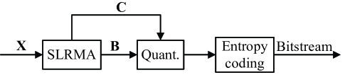
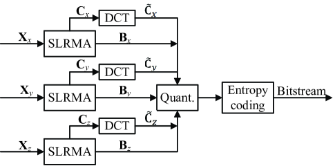
Figure 4: The flowcharts of the proposed SLRMA-based compression schemes for image sets (a) and 3D dynamic meshes (b).

(a) Image set used in Figure 2

(b) Image set I

(c) Image set II

(d) Image set III

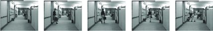
(e) Image set IV

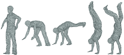
(f) 3D dynamic meshes

Figure 5: Examples of test datasets.

V-A Image Sets

Given a grayscale image set with $n$ images denoted by $\{\mathbf{M}_{i}\in\mathbb{R}^{w\times h}\}_{i=1,2,\cdots,n}$ where $w$ and $h$ are the resolution of the images, respectively, we reshape each image as a column vector and stack them into a matrix denoted by $\mathbf{X}\in\mathbb{R}^{wh\times n}$. As shown in Figure 4(a), our SLRMA-based compression scheme is very simple. It decomposes $\mathbf{X}$ into an extremely sparse matrix $\mathbf{B}$ and a coefficients matrix $\mathbf{C}$. They are then uniformly quantized before the nonzero elements, as well as their locations, are entropy-coded into a bitstream using arithmetic coding.

We tested four grayscale image sets: Image set I: 150 facial images (resolution: $64\times 64$) extracted from the AR dataset [42]; Image set II: 150 facial images (resolution: $65\times 75$) extracted from the Fa of FERET dataset [43]; Image set III: 150 images (resolution: $88\times 72$) extracted from the “carphone” video sequence; Image set IV: 150 images (resolution: $88\times 72$) extracted from the “hall” video sequence. Some data samples are respectively shown in Figures 5(b)-(e). The values of $\rho$, $\alpha$, and $\rho_{max}$ are set to $10^{-4}$, 1.05, and $10^{10}$, respectively. Note that these parameters are insensitive to the size of image sets. The percentage of zero elements of $\mathbf{B}$ is denoted by $p_{B}$, and various $p_{B}$ is obtained by adjusting $\gamma$.

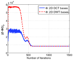
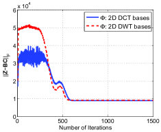
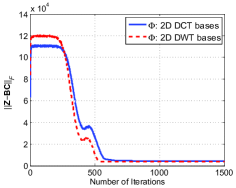
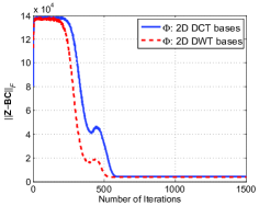
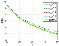
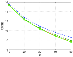
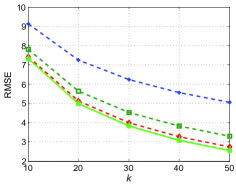
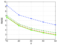
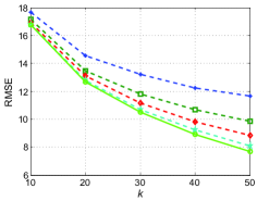
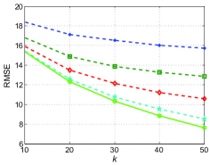
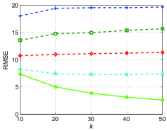
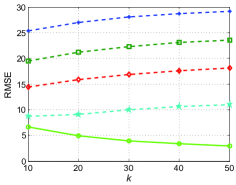
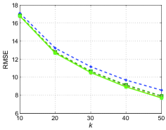
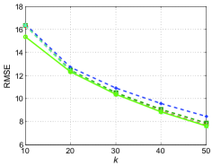
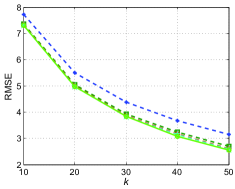
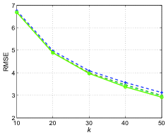
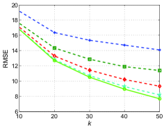
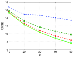
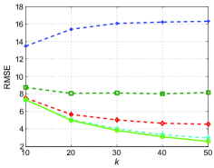
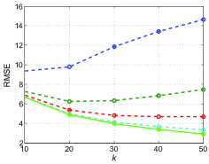
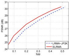
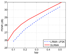
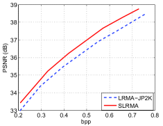
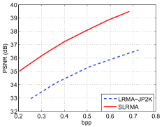
(a) Image set I(b) Image set II (c) Image set III(d) Image set IV

Figure 6: Evaluation of SLRMA on image sets. $1^{st}$ row: convergence verification of SLRMA ($p_{B}=0.6$ and $k=30$); $2^{nd}$row: low-rank approximation performance of SLRMA (DCT) under various $p_{B}$; $3^{rd}$ row: performance of the stepwise method LRMA-DCT under various $p_{B}$; $4^{th}$ row: low-rank approximation performance of SLRMA (DWT) under various $p_{B}$; $5^{th}$ row: performance of the stepwise method LRMA-DWT under various $p_{B}$; $6^{th}$ row: comparison of rate-distortion performance of SLRMA-based and LRMA-JPEG2K, and $\bf\Phi$ is realized by DWT; Note that rows 2-5 share the same legend.

Firstly, we evaluate the convergence and low-rank approximation performance of SLRMA under various $p_{B}$, i.e., the relationship among approximation error, $k$ and $p_{B}$. The approximation error is measured by the Root Mean Square Error (RMSE) between the original data $\mathbf{X}$ and approximate data $\widehat{\mathbf{X}}$, i.e.,

$$\centering{\rm RMSE}=\sqrt{\frac{1}{mn}\left\|\mathbf{X}-\widehat{\mathbf{X}}\right\|_{F}^{2}}.\@add@centering$$ (26)

The SLRAM is validated under two cases, which are denoted by: (i) SLRMA (DCT) in which $\bf{\Phi}$ is set as the 2D DCT matrix, i.e., the Kronecker product of two 1D DCT matrices; (ii) SLRMA (DWT) in which $\bf{\Phi}$ is realized by the 2D DWT matrix obtained as the Kronecker product of two multi-level Haar matrices (3-level for image sets I and II, and 4-level for image sets III and IV). As a comparison, we also present the performance of stepwise methods, namely LRMA-DCT (resp. LRMA-DWT), in which the same DCT (resp. DWT) matrix as SLRMA is applied to columns of $\mathbf{B}$ obtained by LRMA, and then $p_{B}$ percentage of all transformed coefficients with smallest magnitude are set to zero before carrying out the inverse transform.

As the first row of Figure 6 shows, SLRMA empirically converges well, i.e., the objective function is reduced to a stable value after a few iterations. The second and forth rows of Figure 6 verify the excellent low-rank approximation performance of SLRMA, that is, at the same $k$, the approximation error by SLRMA is comparable to that by LRMA, which is the lower bound. Moreover, SLRMA (DWT) is better than SLRMA (DCT) on image sets III and IV since the multi-level DWT has greater potential for sparsly representing images with complex textures than DCT [44]. For image sets I and II, which contain relatively smooth facial images, both DWT and DCT can decorrelate the data well, so that the difference between SLRMA (DWT) and SLRMA (DCT) is very slight. However, the stepwise methods LRMA-DCT and LRMA-DWT, shown in the third and fifth rows, induce much larger approximation error than SLRMA at the same $k$ and $p_{B}$. Finally, we show the rate-distortion performance of the SLRMA-based compression scheme in the sixth row of Figure 6, where we can see that the SLRMA-based method consistently produces higher peak-signal-noise-ratio (PSNR) at the same bit per pixel (bpp). The improvement is up to 3 dB compared to the method in [18], namely LRMA-JP2K, in which the DWT-based JP2K image encoder is employed to encode the basis vectors after LRMA is applied. Figure 7 also compares visual results by SLRMA and LRMA-JP2K, where we can observe that areas around persons marked out by red ovals are obviously blurred for LRMA-JP2K images, but the corresponding images by SLRMA are sharper and visually closer to original images at the same bpp. Last but not least, we believe that our SLRMA-based compression scheme can achieve higher rate-distortion performance by adopting more advanced entropy coding, e.g., context-adaptive binary arithmetic coding (CABAC) [45] and embedded block coding with optimal truncation (EBCOT) [29].

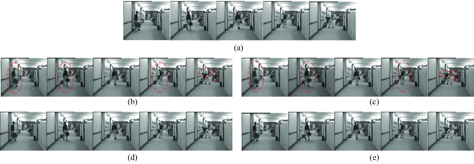
Figure 7: Comparison of visual results on image set. (a) original images from the Image set IV. (b) and (c) compressed ones by the LRMA-JP2K method under 0.38 bpp and 0.21 bpp, respectively; (d) and (e) compressed ones by our SLRMA-based method under 0.38 bpp and 0.21 bpp, respectively.

V-B 3D Dynamic Meshes

Given a 3D dynamic mesh sequence with $m$ vertices and $n$ frames, it can be represented as three matrices $\mathbf{X}_{x}\in\mathbb{R}^{m\times n}$, $\mathbf{X}_{y}\in\mathbb{R}^{m\times n}$, $\mathbf{X}_{z}\in\mathbb{R}^{m\times n}$, corresponding to the $x-$, $y-$, and $z-$dimensions of vertices, respectively, and each column of $\mathbf{X}_{d}~{}~{}(d:=\{x,y,z\})$ corresponds to the $d-$dimension of vertices of one frame. The SLRMA-based compression scheme is shown in Figure 4(b), where $\mathbf{X}_{d}$ is firstly factored into $\mathbf{B}_{d}$ and $\mathbf{C}_{d}$ using SLRMA. Different from image sets, 3D dynamic mesh sequences consist of successive frames of objects in motion, so that each row of $\mathbf{X}_{d}$, corresponding to the $d$-dimensional trajectory of one vertex, is a relatively smooth curve, indicating strong coherence. After the SLRMA, such coherence still exists in rows of $\mathbf{C}_{d}$ [22]. For example, Figure 8 plots several rows of $\mathbf{C}_{d}$, where their relative smoothness is verified. This can be easily explained using the analysis for intra-correlation of $\mathbf{B}$ of LRMA along the row space of $\mathbf{X}$. To further reduce this temporal coherence, 1D DCT is separately performed on rows of $\mathbf{C}_{d}$, i.e.,

$$\centering\widetilde{\mathbf{C}}_{d}=\mathbf{U}_{dct}^{\textsf{T}}\mathbf{C}_{d}^{\textsf{T}},\@add@centering$$ (27)

where $\mathbf{U}_{dct}\in\mathbb{R}^{n\times n}$ stands for the 1D DCT matrix, and each column corresponds to one frequency. Lastly, the nonzero entries of uniformly quantized $\mathbf{B}_{d}$ and $\widetilde{\mathbf{C}}_{d}$ as well as their locations are entropy-coded using arithmetic coding.

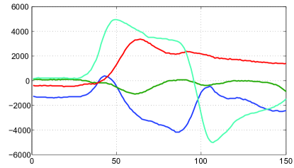
Figure 8: Illustration of the coherence within rows of $\mathbf{C}_{d}$.

We take four 3D dynamic mesh sequences from [46], including “Wheel” (2501 vertices), “Handstand” (2501 vertices), “Skirt” (2502 vertices), and “Dance” (1502 vertices). Each sequence has 150 frames. Some samples are shown in Figure 5(f). The values of $\rho$, $\alpha$, and $\rho_{max}$ are set to $10^{7}$, 1.003, and $10^{12}$, respectively. The orthogonal matrix $\bf{\Phi}$ is realized by the GT, as explained in Section III-B, and can be computed according to the topology of 3D meshes. Note that the three dimensions are equally treated, i.e., the same $k$ and $p_{B}$ are used.

The empirical convergence of SLRMA is verified again in the first row of Figure 9. The low-rank approximation performance of SLRMA is shown in the second row of Figure 9, where we can see that at the same $k$, SLRMA produces comparable RMSEs as LRMA even when the value of $p_{B}$ increases up to 0.8. However, the stepwise method denoted by LRMA-GT produces much larger RMSEs. See the third row of Figure 9. Note that $\mathbf{X}=[\mathbf{X}_{x};\mathbf{X}_{y};\mathbf{X}_{z}]\in\mathbb{R}^{3m\times n}$ and $\widehat{\mathbf{X}}=[\widehat{\mathbf{X}}_{x};\widehat{\mathbf{X}}_{y};\widehat{\mathbf{X}}_{z}]\in\mathbb{R}^{3m\times n}$ when computing the approximation error using (26).

Finally, we evaluate the rate-distortion performance of the SLRMA-based compression method. The compression distortion is measured by the widely-adopted KG error [22], defined as

$$\centering{\rm KG~{}error}=100\times\frac{\left\|\mathbf{X}-\widehat{\mathbf{X}}\right\|_{F}}{\left\|\mathbf{X}-E(\mathbf{X})\right\|_{F}},\@add@centering$$ (28)

where $E(\mathbf{X})$ is an average matrix of the same size as $\mathbf{X}$, of which the $j$-th column is $((\overline{\mathbf{x}}_{x})_{j}[1~{}\cdots~{}1]~{}(\overline{\mathbf{x}}_{y})_{j}[1~{}\cdots~{}1]~{}(\overline{\mathbf{x}}_{z})_{j}[1~{}\cdots~{}1])^{\textsf{T}}$ with $(\overline{\mathbf{x}}_{d})_{j}$ being the average of $(\mathbf{x}_{d})_{j}$. The bitrate is measured in bit per frame per vertex (bpfv). The overall compression performance of our scheme is affected by three parameters: $k$ (the number of basis vectors), $p_{B}$ (the percentage of zero elements of $\mathbf{B}$), and the quantization parameter. Currently, we use exhaustive search to determine their optimal combination. One can also employ the method in [47] or build rate and distortion models in terms of the three parameters, like [3], to speed up this process in practice. We compare with Váša’s scheme in [24], which is LRMA-based and represents the state-of-the-art performance.

The forth row of Figure 9 shows typical rate-distortion curves for our scheme as well as Váša’s, where it can be seen that for “Dance” and “Skirt”, our method produces much smaller distortion than Váša’s at the same bpfv, especially at relatively small bpfvs. With respect to “Handstand” and “Wheel”, the rate-distortion curves of Váša’s are not given since Váša’s method can only work on manifold-meshes, but sequences “Handstand” and “Wheel” consists of non-manifold-meshes. Our scheme is independent of topology, which is an additional advantage. Finally, some visual results are shown in Figures 10 and 11 to further demonstrate the performance of our scheme, where we can observe that the decompressed frames are still close to the original ones and their quality are reasonable even when the bpfv is equal to 0.25.

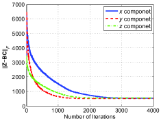
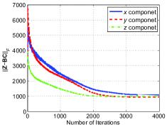
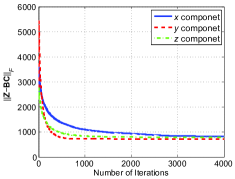
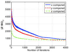
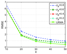
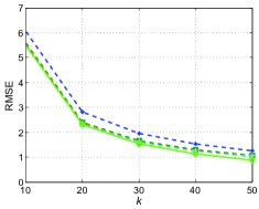
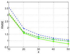
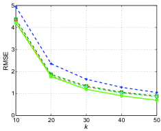
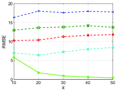
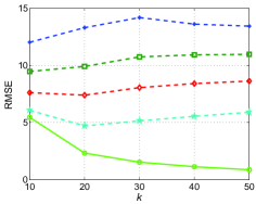
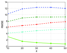
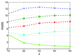
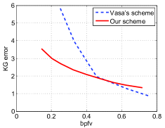
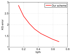
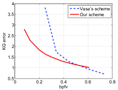
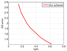
(a) “Dance”(b) “Handstand” (c) “Skirt”(d) “Wheel”

Figure 9: Evaluation of SLRMA on 3D dynamic meshes. $1^{st}$ row: the convergence verification of SLRMA ($p_{B}=0.6$ and $k=30$); $2^{nd}$ row: low-rank approximation performance of SLRMA (GT) at various $p_{B}$; $3^{rd}$ row: performance of the stepwise method LRMA-GT at various $p_{B}$; $4^{th}$ row: rate-distortion performance of our SLRMA-based method and the state-of-the-art method. Note that rows 2-3 share the same legend.

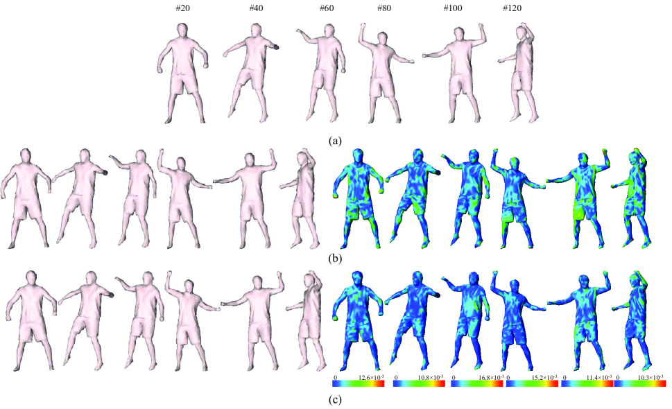
Figure 10: Visual results on dynamic meshes. (a) shows six frames of the “Dance” dynamic mesh. (b) and (c) show decoded frames with bpfv 0.25 and 0.45, respectively. The error is measured by RMS [48] with respect to the bounding box diagonal and visualized using colormap.

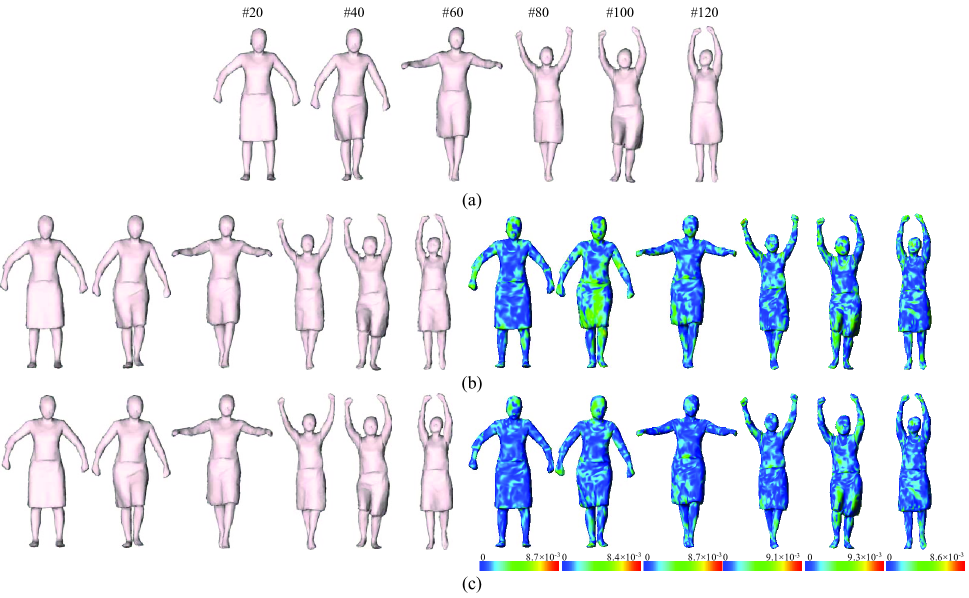
Figure 11: Visual results on dynamic meshes. (a) shows six frames of the “Skirt” dynamic mesh. (b) and (c) show decoded frames with bpfv 0.25 and 0.45, respectively. The error is measured by RMS [48] with respect to the bounding box diagonal and visualized using colormap.

VI Conclusion and Future Work

We presented sparse low-rank matrix approximation for effective data compression. In contrast to the conventional LRMA, SLRMA is able to explore both the intra- and inter-coherence among data simultaneously, producing extremely sparse basis functions. We formulated the SLRMA problem as a constrained optimization problem and solved it using the inexact augmented Lagrangian multiplier method. Although the optimization problem is non-convex, we observed that our method empirically converges well on real-world data, such as image sets and 3D dynamic meshes. Also, SLRMA exhibits excellent low-rank approximation performance, i.e., at the same rank, comparable approximation error as LRMA is produced even when 80% entries of basis vectors are zero. Moreover, at the same bitrate, the SLRMA-based compression schemes can reduce distortion by up to 53% for 3D dynamic meshes and improve PSNR by up to 3 dB for image sets compared with existing methods.

In the future, we would like to further investigate the potential of SLRMA to compress other types of data (e.g., EEG signals). We also believe that SLRMA can be applied to other applications, such as patch-based image and video denoising, where both the similarity among patches (i.e., low-rank characteristic) and spatial structure of patches (i.e., the sparseness of patches with respect to particular bases) can be jointly taken into account.

References

- [1] N. Halko, P.-G. Martinsson, and J. A. Tropp, “Finding structure with randomness: Probabilistic algorithms for constructing approximate matrix decompositions,” SIAM review, vol. 53, no. 2, pp. 217–288, 2011.
- [2] Z. Gu, W. Lin, B.-S. Lee, and C. Lau, “Low-complexity video coding based on two-dimensional singular value decomposition,” IEEE Trans. Image Processing, vol. 21, no. 2, pp. 674–687, 2012.
- [3] J. Hou, L.-P. Chau, N. Magnenat-Thalmann, and Y. He, “Compressing 3-d human motions via keyframe-based geometry videos,” IEEE Transactions on Circuits and Systems for Video Technology, vol. 25, no. 1, pp. 51–62, Jan 2015.
- [4] E. J. Candès, X. Li, Y. Ma, and J. Wright, “Robust principal component analysis?” Journal of the ACM, vol. 58, no. 3, p. 11, 2011.
- [5] J. Wen, Y. Xu, J. Tang, Y. Zhan, Z. Lai, and X. Guo, “Joint video frame set division and low-rank decomposition for background subtraction,” IEEE Trans. Circuits and Systems for Video Technology, vol. 24, no. 12, pp. 2034–2048, 2014.
- [6] G. Liu, Z. Lin, S. Yan, J. Sun, Y. Yu, and Y. Ma, “Robust recovery of subspace structures by low-rank representation,” IEEE Trans. Pattern Analysis and Machine Intelligence, vol. 35, no. 1, pp. 171–184, 2013.
- [7] Y. Zhang, Z. Jiang, and L. S. Davis, “Learning structured low-rank representations for image classification,” in Proc. IEEE Computer Vision and Pattern Recognition (CVPR). IEEE, 2013, pp. 676–683.
- [8] H. Ji, S. Huang, Z. Shen, and Y. Xu, “Robust video restoration by joint sparse and low rank matrix approximation,” SIAM Journal on Imaging Sciences, vol. 4, no. 4, pp. 1122–1142, 2011.
- [9] Z. Wang, H. Li, Q. Ling, and W. Li, “Robust temporal-spatial decomposition and its applications in video processing,” IEEE Trans. Circuits and Systems for Video Technology, vol. 23, no. 3, pp. 387–400, 2013.
- [10] Y. Peng, A. Ganesh, J. Wright, W. Xu, and Y. Ma, “Rasl: Robust alignment by sparse and low-rank decomposition for linearly correlated images,” IEEE Trans. Pattern Analysis and Machine Intelligence, vol. 34, no. 11, pp. 2233–2246, 2012.
- [11] F. Cao, M. Cai, and Y. Tan, “Image interpolation via low-rank matrix completion and recovery,” IEEE Trans. Circuits and Systems for Video Technology, vol. 25, no. 8, pp. 1261–1270, 2015.
- [12] Y. Dai, H. Li, and M. He, “Projective multiview structure and motion from element-wise factorization,” IEEE Trans. Pattern Analysis and Machine Intelligence, vol. 35, no. 9, pp. 2238–2251, 2013.
- [13] ——, “A simple prior-free method for non-rigid structure-from-motion factorization,” International Journal of Computer Vision, vol. 107, no. 2, pp. 101–122, 2014.
- [14] D. Meng, Z. Xu, L. Zhang, and J. Zhao, “A cyclic weighted median method for l1 low-rank matrix factorization with missing entries.” in Proc. AAAI, 2013, pp. 1–7.
- [15] X. Zhou, C. Yang, H. Zhao, and W. Yu, “Low-rank modeling and its applications in image analysis,” ACM Computing Surveys (CSUR), vol. 47, no. 2, p. 36, 2014.
- [16] J.-F. Yang and C.-L. Lu, “Combined techniques of singular value decomposition and vector quantization for image coding,” IEEE Trans. Image Processing, vol. 4, no. 8, pp. 1141–1146, 1995.
- [17] H. Ochoa and K. Rao, “A hybrid dwt-svd image-coding system (hdwtsvd) for monochromatic images,” in Proc. SPIE Image and Video Communications and Processing, 2003, pp. 1056–1066.
- [18] Q. Du and J. E. Fowler, “Hyperspectral image compression using jpeg2000 and principal component analysis,” IEEE Geoscience and Remote Sensing Letters, vol. 4, no. 2, pp. 201–205, 2007.
- [19] C. Chen, J. Cai, W. Lin, and G. Shi, “Incremental low-rank and sparse decomposition for compressing videos captured by fixed cameras,” Journal of Visual Communication and Image Representation, vol. 26, pp. 338–348, 2015.
- [20] J. Hou, L.-P. Chau, M. Zhang, N. Magnenat-Thalmann, and Y. He, “A highly efficient compression framework for time-varying 3-d facial expressions,” IEEE Trans. Circuits and Systems for Video Technology, vol. 24, no. 9, pp. 1541–1553, Sept 2014.
- [21] M. Alexa and W. Müller, “Representing animations by principal components,” Computer Graphics Forum, vol. 19, no. 3, pp. 411–418, 2000.
- [22] Z. Karni and C. Gotsman, “Compression of soft-body animation sequences,” Computers & Graphics, vol. 28, no. 1, pp. 25–34, 2004.
- [23] L. Váša and V. Skala, “Geometry-driven local neighbourhood based predictors for dynamic mesh compression,” Computer Graphics Forum, vol. 29, no. 6, pp. 1921–1933, 2010.
- [24] L. Váša, S. Marras, K. Hormann, and G. Brunnett, “Compressing dynamic meshes with geometric laplacians,” Computer Graphics Forum, vol. 33, no. 2, pp. 145–154, 2014.
- [25] J. Hou, L. Chau, N. Magnenat-Thalmann, and Y. He, “Human motion capture data tailored transform coding,” IEEE Trans. Visualization and Computer Graphics, vol. 21, no. 7, pp. 848–859, 2015.
- [26] Q. Li, H. Jianming, and Z. Yi, “A flow volumes data compression approach for traffic network based on principal component analysis,” in Proc. IEEE Intelligent Transportation Systems Conference (ITSC), 2007, pp. 125–130.
- [27] M. T. Asif, S. Kannan, J. Dauwels, and P. Jaillet, “Data compression techniques for urban traffic data,” in Proc. IEEE Symposium on Computational Intelligence in Vehicles and Transportation Systems (CIVTS), 2013, pp. 44–49.
- [28] M. Asif, K. Srinivasan, N. Mitrovic, J. Dauwels, and P. Jaillet, “Near-lossless compression for large traffic networks,” IEEE Trans. Intelligent Transportation Systems, vol. PP, no. 99, pp. 1–12, 2014.
- [29] A. Skodras, C. Christopoulos, and T. Ebrahimi, “The jpeg 2000 still image compression standard,” IEEE Signal Processing Magazine, vol. 18, no. 5, pp. 36–58, 2001.
- [30] T. Wiegand, G. Sullivan, G. Bjontegaard, and A. Luthra, “Overview of the h.264/avc video coding standard,” IEEE Trans. Circuits and Systems for Video Technology, vol. 13, no. 7, pp. 560–576, July 2003.
- [31] J.-H. Heu, C.-S. Kim, and S.-U. Lee, “Snr and temporal scalable coding of 3-d mesh sequences using singular value decomposition,” Journal of Visual Communication and Image Representation, vol. 20, no. 7, pp. 439–449, 2009.
- [32] M. Sattler, R. Sarlette, and R. Klein, “Simple and efficient compression of animation sequences,” in Proc. ACM SIGGRAPH/Eurographics SCA, 2005, pp. 209–217.
- [33] L. Váša and V. Skala, “Coddyac: Connectivity driven dynamic mesh compression,” in Proc. IEEE 3DTV, 2007, pp. 1–4.
- [34] ——, “Cobra: Compression of the basis for pca represented animations,” Computer Graphics Forum, vol. 28, no. 6, pp. 1529–1540, 2009.
- [35] E. Kokiopoulou, J. Chen, and Y. Saad, “Trace optimization and eigenproblems in dimension reduction methods,” Numerical Linear Algebra with Applications, vol. 18, no. 3, pp. 565–602, 2011.
- [36] I. Markovsky and K. Usevich, Low rank approximation. Springer, 2012.
- [37] H. Zhang, O. Van Kaick, and R. Dyer, “Spectral mesh processing,” Computer Graphics Forum, vol. 29, no. 6, pp. 1865–1894, 2010.
- [38] C. Zhang and D. Florêncio, “Analyzing the optimality of predictive transform coding using graph-based models,” IEEE Signal Processing Letters, vol. 20, no. 1, pp. 106–109, 2013.
- [39] R. Wang, Introduction to orthogonal transforms: with applications in data processing and analysis. Cambridge University Press, 2012.
- [40] Z. Lin, M. Chen, and Y. Ma, “The augmented lagrange multiplier method for exact recovery of corrupted low-rank matrices,” arXiv preprint arXiv:1009.5055, 2010.
- [41] R. Lai and S. Osher, “A splitting method for orthogonality constrained problems,” Journal of Scientific Computing, vol. 58, no. 2, pp. 431–449, 2014.
- [42] A. M. Martinez, “The ar face database,” CVC Technical Report, vol. 24, 1998.
- [43] P. J. Phillips, H. Moon, S. A. Rizvi, and P. J. Rauss, “The feret evaluation methodology for face-recognition algorithms,” IEEE Trans. Pattern Analysis and Machine Intelligence, vol. 22, no. 10, pp. 1090–1104, 2000.
- [44] K. R. Rao and P. C. Yip, The transform and data compression handbook. CRC press, 2000.
- [45] D. Marpe, H. Schwarz, and T. Wiegand, “Context-based adaptive binary arithmetic coding in the h. 264/avc video compression standard,” IEEE Trans. Circuits and Systems for Video Technology, vol. 13, no. 7, pp. 620–636, 2003.
- [46] J. Gall, C. Stoll, E. De Aguiar, C. Theobalt, B. Rosenhahn, and H.-P. Seidel, “Motion capture using joint skeleton tracking and surface estimation,” in Proc. IEEE CVPR, 2009, pp. 1746–1753.
- [47] O. Petřík and L. Váša, “Finding optimal parameter configuration for a dynamic triangle mesh compressor,” in Proc. Articulated Motion and Deformable Objects. Springer, 2010, pp. 31–42.
- [48] P. Cignoni, C. Rocchini, and R. Scopigno, “Metro: measuring error on simplified surfaces,” Computer Graphics Forum, vol. 17, no. 2, pp. 167–174, 1998.