Almost Strong Consistency: “Good Enough” in Distributed Storage Systems

Abstract

A consistency/latency tradeoff arises as soon as a distributed storage system replicates data. For low latency, modern storage systems often settle for weak consistency conditions, which provide little, or even worse, no guarantee for data consistency. In this paper we propose the notion of almost strong consistency as a better balance option for the consistency/latency tradeoff. It provides both deterministically bounded staleness of data versions for each read and probabilistic quantification on the rate of “reading stale values”, while achieving low latency. In the context of distributed storage systems, we investigate almost strong consistency in terms of 2-atomicity. Our 2AM (2-Atomicity Maintenance) algorithm completes both reads and writes in one communication round-trip, and guarantees that each read obtains the value of within the latest 2 versions. To quantify the rate of “reading stale values”, we decompose the so-called “old-new inversion” phenomenon into concurrency patterns and read-write patterns, and propose a stochastic queueing model and a timed balls-into-bins model to analyze them, respectively. The theoretical analysis not only demonstrates that “old-new inversions” rarely occur as expected, but also reveals that the read-write pattern dominates in guaranteeing such rare data inconsistencies. These are further confirmed by the experimental results, showing that 2-atomicity is “good enough” in distributed storage systems by achieving low latency, bounded staleness, and rare data inconsistencies.

1 Introduction

Distributed storage systems [13] [15] [14] [10] are considered as integral and fundamental components of modern Internet services such as e-commerce and social networks. They are expected to be fast, always available, highly scalable, and network-partition tolerant. To this end, modern distributed storage systems typically replicate their data across different machines and even across multiple data centers, at the expense of introducing data inconsistency.

More importantly, as soon as a storage system replicates data, a tradeoff between consistency and latency arises [4]. This consistency/latency tradeoff arguably has been highly influential in system design because it exists even when there are no network partitions [4]. In distributed storage systems, latency is widely regarded as a critical factor for a large class of applications. For example, the experiments from Google [12] demonstrate that increasing web search latency 100 to 400 ms reduces the daily number of searches per user by 0.2% to 0.6%. Therefore, most storage systems (and applications built on them) are designed for low latency in the first place. They often sacrifice strong consistency and settle for weaker ones, such as eventual consistency [15], per-record timeline consistency [14], and causal consistency [23]. However, such weak consistency models usually provide little, or even worse, no guarantee for data consistency. More specifically, they neither make any deterministic guarantee on the staleness of the data returned by reads nor provide probabilistic hints on the rate of violations with respect to the desired strong consistency.

In this paper we propose the notion of almost strong consistency as a better balance option for the consistency/latency tradeoff. The implication of the term “almost” is twofold. On one hand, it provides deterministically bounded staleness of data versions for each read. Thus, the users are confident that out-of-date data is still useful as long as they can tolerate certain staleness. On the other hand, it further provides probabilistic quantification on the low rate of “reading stale values”. This ensures that the users are actually accessing up-to-date data most of the time.

We illustrate the idea of almost strong consistency by an exemplar mobile-app-based taxi transportation system. In this system, each taxi periodically reports its location data to the data server. Due to the natural locality of the update and request of location data, the city is partitioned into multiple areas and a data server is deployed in each area. The location data is replicated among all the data servers. Thus the users all over the city can request the location data via a mobile application like Uber [3]. Though consistency is a desirable property, in this application the user may be more concerned of how long he has to wait before his query can be served. We argue that the application may be willing to trade certain consistency for low latency, as long as the inconsistency is bounded and the application can still access up-to-date data most of the time [20].

In the context of distributed storage systems, we investigate almost strong consistency in terms of 2-atomicity. By instantiating the abstract notion of almost strong consistency, the 2-atomicity semantics also includes two essential parts as elaborated below.

First, the 2-atomicity semantics guarantees that the value returned by each read is one of the latest 2 versions, besides admitting an implementation with low latency. By “low latency” we mean that both reads and writes complete in one communication round-trip. Theoretically, it has been proved impossible to achieve low latency while enforcing each read to return the latest data version, as required in atomicity [21] [19], given that a minority of replicas may fail [16]. For example, the ABD algorithm [7] for emulating atomic registers requires each read to complete in two round-trips. This impossibility result justifies the relaxed consistency semantics of 2-atomicity. In the transportation system example above, the taxi location data can still be useful if the data returned is no more stale than the previous version to the latest one. This is mainly because the location data cannot change abruptly and the taxi frequently updates its location in this scenario.

Second, the 2-atomicity semantics provides probabilistic quantification on the rate of violations of atomicity. In data storage systems, atomicity is widely used as the formal definition of strongly consistent or up-to-date data access. By bounding the probability of violating atomicity, the 2-atomicity semantics provides another orthogonal perspective for expressing how strong consistency is “almost” guaranteed. In our example above, since the user may request the location data of a number of taxies, the inconsistency data may not affect the quality of service experienced by the user, as long as only a small portion of the query return slightly stale data.

Our 2AM (2-Atomicity Maintenance) algorithm for maintaining 2-atomicity in distributed storage systems completes both reads and writes in one communication round-trip, and guarantees that each read obtains the value of within the latest 2 versions. To quantify the rate of “reading stale values”, we decompose the so-called “old-new inversion” phenomenon into two patterns: concurrency pattern and read-write pattern. We then propose a stochastic queueing model and a timed balls-into-bins model to analyze the two patterns, respectively. The theoretical analysis not only demonstrates that “old-new inversions” rarely occur as expected, but also reveals that the read-write pattern dominates in guaranteeing such rare violations.

We have also implemented a prototype data storage system among mobile phones, which provides 2-atomic data access based on the 2AM algorithm and atomic data access based on the ABD algorithm. The read latency in our 2AM algorithm has been significantly reduced, compared to that in the ABD algorithm. More importantly, the experimental results have confirmed our theoretical analysis above. Specifically, the proportion of old-new inversions incurred in the 2AM algorithm is typically less than 0.1‰, and the proportion of read-write patterns among concurrency patterns (e.g., about 0.1‰ in some setting) is much less than that of concurrency patterns themselves (e.g., more than $50\%$ in the same setting). Thus 2-atomicity is “good enough” in distributed storage systems by achieving low latency, bounded staleness, and rare atomicity violations.

The remainder of the paper is organized as follows. Section 2 proposes the notion of almost strong consistency and discusses how to define it in terms of 2-atomicity in the context of distributed storage systems. Section 3 presents the 2AM (2-Atomicity Maintenance) algorithm which achieves deterministically bounded staleness. Section 4 is concerned with the theoretical analysis of the atomicity violations incurred in the 2AM algorithm. Section 5 presents the prototype data storage system and experimental results. Section 6 reviews the related work. Section 7 concludes the paper.

2 Almost Strong Consistency

In this section, we propose the notion of almost strong consistency, and instantiate it in terms of 2-atomicity, in the context of distributed storage systems.

2.1 Generic Notion of Almost Strong Consistency

The distributed storage system consists of an arbitrary number of $N$ clients and a fixed number $n$ of server replicas (or replicas, for short) that communicate through message-passing (Figure 1). Each replica maintains a set of replicated key-value pairs (also referred to as registers in the sequel).

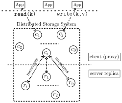
Figure 1: Distributed storage system model.

The distributed storage system supports two operations to upper-layer applications: 1)  storing a value associated with a key, denoted write(key,value); and 2)  retrieving a value associated with a key, denoted value $\leftarrow$ read(key). Clients serve as the proxies for applications by invoking read/write operations on the registers and communicating with replicas on behalf of them. Being replicated, different versions of the same register may co-exist. The concept of consistency models is then introduced to constrain the possible data versions that are allowed to be returned by each read. Particularly, strong consistency requires each read to obtain the latest data version according to some sequential order.

The notion of almost strong consistency generalizes the traditional strong consistency by allowing stale data versions to be read. That is,

1. It provides deterministically bounded staleness of data versions for each read;

2. It provides probabilistic quantification on the rate of “reading stale values”.

2.2 Almost Strong Consistency in Terms of 2-Atomicity

In the context of distributed storage systems, we investigate almost strong consistency in terms of 2-atomicity. As preliminaries, we first review atomicity [8]. From the view of clients, each operation is associated with two events: an invocation event and a response event. For a read (on a specific key), the invocation is denoted read(key), and its response has the form ack(value), returning some value to the client. For a write, the invocation is denoted write(key, value), and its response is an ack, indicating its completion. We assume an imaginary global clock and all the events are time-stamped with respect to it [21]. Among all the writes, we posit, for each register, the existence of a special one which writes the initial value, at the very beginning of the imaginary global clock.

An execution $\sigma$ of the distributed storage system is a sequence of invocations and responses. An operation $o_{1}$ precedes another operation $o_{2}$, denoted $o_{1}\prec_{\sigma}o_{2}$ (or $o_{1}\prec o_{2}$ if $\sigma$ is clear or irrelevant), if and only if the response of $o_{1}$ occurs in $\sigma$ before the invocation of $o_{2}$. Two operations are considered concurrent if neither of them precedes the other. An execution $\sigma$ is said well-formed if each client invokes at most one operation at a time, that is, for each client $p_{i}$, $\sigma|i$ (the subsequence of $\sigma$ restricted on $p_{i}$) consists of alternating invocations and matching responses, beginning with an invocation. A well-formed execution $\sigma$ is sequential if for each operation in $\sigma$, its invocation is immediately followed by its response.

Intuitively, atomicity requires each operation to appear to take effect instantaneously at some point between its invocation and its response. More precisely,

Definition 1.

A storage system satisfies atomicity [8] if, for each of its well-formed executions $\sigma$, there exists a permutation $\pi$ of all the operations in $\sigma$ such that $\pi$ is sequential and

• $[$real-time requirement$]$ If $o_{1}\prec_{\sigma}o_{2}$, then $o_{1}$ appears before $o_{2}$ in $\pi$; and

• $[$read-from requirement$]$ Each read returns the value written by the most recently preceding write in $\pi$ on the same key, if there is one, and otherwise returns its initial value.

The semantics of 2-atomicity is adapted from that of atomicity by relaxing its read-from requirement to allow stale values to be read.

Definition 2.

A storage system satisfies 2-atomicity if, for each of its well-formed executions $\sigma$, there exists a permutation $\pi$ of all the operations in $\sigma$ such that $\pi$ is sequential and

• $[$real-time requirement$]$ If $o_{1}\prec_{\sigma}o_{2}$, then $o_{1}$ appears before $o_{2}$ in $\pi$; and

• $[$weak read-from requirement$]$ Each read returns the value written by one of the latest two preceding writes in $\pi$ on the same key.

In terms of 2-atomicity, the notion of almost strong consistency can then be instantiated as follows.

1. Besides admitting an implementation with low latency, it guarantees that each read obtains the value of within the latest 2 versions;

2. It provides probabilistic quantification on the rate of actually reading the stale data version.

Sections 3 and 4 are concerned with these two aspects, respectively.

3 Achieving 2-Atomicity

In this section, we present the 2AM (2-Atomicity Maintenance) algorithm for emulating 2-atomic, Single-Writer Multi-Reader (SWMR) registers. It completes both reads and writes in one round-trip, and guarantees that each read obtains the value of within the latest 2 versions.

Despite its simplicity, SWMR registers are useful in a wide range of applications, especially where the shared data has its natural “owner”. Moreover, multiple SWMR registers can be used in group. The typical setting is that each process has its “own” register i.e., only the owner process can write this register, while all processes can read all registers. Multiple processes can communicate with each other by writing its own register and reading other registers. A possible alternative is to use Multi-Writer Multi-Reader (MWMR, for short) registers. Compared with using MWMR registers, using SWMR register in group may be more compatible with the application logic, and the implementation is less complex and has better maintainability.

3.1 The 2AM (2-Atomicity Maintenance) Algorithm

We use the asynchronous, non-Byzantine model, in which: 1) Messages can be delayed, lost, or delivered out of order, but they are not corrupted; and 2) An arbitrary number of clients may crash while only a minority of replicas may crash.

The 2AM algorithm is an adaptation from that for atomicity [7]. It makes use of versioning. Specifically, for each write(key, value), the writer associates a version with the key-value pair. Each replica replaces a key-value pair it currently holds whenever a larger version with the same key is received. When reading from a key, a client tries to retrieve the value with the largest version. Since there is only one writer, versions (for each key) can be chosen totally ordered using its local sequence numbers.

At its core, the algorithm is stated in terms of the majority quorum systems in the way that each operation is required to contact any majority of the replicas to proceed. Specifically,

• write(key, value): To write a value on a specific key, the single writer first generates a larger version than those it has ever used, associates it with the key-value pair, sends the versioned key-value pair to all the replicas, and waits for acknowledgments from a majority of them.

• read(key): To read from a specific key, the reader first queries and collects a set of versioned key-value pairs from a majority of the replicas, from which it chooses the one with the largest version to return.

As mentioned before, each replica replaces its key-value pair whenever a larger version with the same key from a write is received. Besides, it responds to the queries from reads with the versioned key-value pair it currently holds.

The pseudo-code for read and write operations and the replicas appears in Algorithm 1. Notice that the read here does not spend a second round-trip propagating the returned value (along with its version) to a majority of the replicas, in contrast to that in [7]. The second round-trip in [7] (often referred to as the “write back” phase) is required to avoid the “old-new inversion” phenomenon [16], [6]. An “old-new inversion” witnesses a violation of atomicity, where two non-overlapping reads, both overlapping a write, obtain out-of-order values. In the 2AM algorithm, we have intentionally ignored the “write back” phase. In the following subsection, we prove that the 2AM algorithm indeed achieves the emulation of 2-atomic, single-writer multi-reader registers.

Algorithm 1 The 2AM (2-Atomicity Maintenance) algorithm for 2-atomic, single-writer multi-reader registers.

1:procedure write(key,value) $\triangleright$ for the writer

2:     increment version for this key

3:     pfor each replica $s$ $\triangleright$ pfor is a parallel for

4:      send $[\textsc{update}\texttt{,key,value,version}]$ to $s$

5:     wait for $[\textsc{ack}]$s from a majority of replicas

1:procedure read(key) $\triangleright$ for each reader

2:     $results\leftarrow\emptyset$

3:     pfor each replica $s$

4:      send $[\textsc{query}\texttt{,key}]$ to $s$

5:      obtain $result\leftarrow[\texttt{k,val,ver}]$ from $s$

6:      $results\leftarrow results\cup\{result\}$

7:     until a majority of replicas respond

8:     return val with the largest ver in $results$

9:$[\texttt{k,val,ver}]:$ local versioned key-value pairs $\triangleright$ The following procedure is executed in an uninterrupted way. Assume that msg is from client $p_{i}$.

1:procedure Upon(msg) $\triangleright$ for each replica

2:     if msg instanceof $[\textsc{query}\texttt{,key}]$

3:          send $[\texttt{k,val,ver}]$ with $\texttt{k}=\texttt{key}$ to client $p_{i}$

4:     end if

5:     if msg instanceof $[\textsc{update}\texttt{,key,value,version}]$

6:         pick $[\texttt{k,val,ver}]$ with $\texttt{k}=\texttt{key}$

7:         if $\texttt{ver}<\texttt{version}$

8:              $\texttt{val}\leftarrow\texttt{value}$

9:              $\texttt{ver}\leftarrow\texttt{version}$

10:         end if

11:         send [ack] to client $p_{i}$

12:     end if

3.2 Correctness Proof of the 2AM Algorithm

We aim to prove that, in the 2AM algorithm, the value returned by each read is of one of the latest 2 versions. It is basically a case-by-case analysis, concerning the partial order among and the semantics of the read/write operations.

Theorem 1

The 2AM algorithm achieves the emulation of 2-atomic, single-writer multi-reader registers.

Proof.

First of all, we notice that 2-atomicity, like atomicity, is a local property [19]. Therefore, we can prove the correctness of the 2AM algorithm by reasoning independently about each individual register accessed in an execution. Without loss of generality, we assume that all the operations involved in the following correctness proof are performed on the same register.

According to the definition of 2-atomicity (Definition 2), it suffices to identify a permutation $\pi$ of any execution of the 2AM algorithm, and to prove that $\pi$ is sequential and satisfies both the “real-time requirement” and the “weak read-from requirement”.

For any execution $\sigma$, we obtain its permutation $\pi$ in the following manner:

• All the write operations issued by the single writer are totally ordered according to the versions they use.

• The read operations are scheduled one by one in order of their invocation time: A read $r$ that reads from a write $w$ is scheduled immediately after both $w$ and all the read operations preceding $r$ in the sense of $\prec_{\sigma}$ (which have already been scheduled).

Obviously, this permutation $\pi$ is sequential and satisfies the “real-time requirement” of 2-atomicity. It remains to show that it satisfies the “weak read-from requirement” for each read as well. This argument involves a case-by-case analysis, concerning the partial order among and the semantics of the read/write operations.

Here and in the sequel, we use the following notations: For an operation $o$, let $o_{st}$ denote its start time (i.e., the time of its invocation event), $o_{ft}$ its finish time (i.e., the time of its response event), and $[o_{st},o_{ft}]$ its time interval (Figure 2 for an example). We also write $r=R(w)$ to denote the “read-from” relation in which the read $r$ reads from the write $w$.

For any read operation $r$, we consider two cases according to whether there are concurrent write operations with it in the execution $\sigma$.

Case 1: There is no concurrent write with $r$. According to the 2AM algorithm (Algorithm 1), especially due to the mechanism of the majority quorum systems, the read $r$ must read from its most recently preceding write $w$, and hence in $\pi$, it is scheduled between $w$ and the next write.

Case 2: There are concurrent writes with $r$, among which the leftmost one is denoted $w$. Notice that $r_{st}\in[w_{st},w_{ft}]$ holds for $w$. There are two sub-cases according to the write from which $r$ reads.

Case 2.1: $r$ reads from some concurrent write. In this case, $r$ is scheduled in $\pi$ between this write and its next one.

Case 2.2: $r$ reads from its most recently preceding write in $\sigma$ (denoted $w^{\prime}$). Notice that Case 2.1 and Case 2.2 are exhaustive since $r$ cannot read from any earlier writes than $w^{\prime}$ due to the mechanism of the majority quorum systems. To form an “old-new inversion”, there must be at least two read operations. Therefore, in Case 2.2 (shown in Figure 2) we now consider other read operations (than $r$).

Case 2.2.1: There is no read $r^{\prime}$ that precedes $r$ in $\sigma$ and is concurrent with $w$. Formally, $\nexists r^{\prime}:r^{\prime}_{ft}\in[w_{st},r_{st}]$. In $\pi$, $r$ is scheduled between $w^{\prime}$ and its next write (i.e., $w$).

Case 2.2.2: There is some read $r^{\prime}$ that precedes $r$ and is concurrent with $w$. Formally, $\exists r^{\prime}:r^{\prime}_{ft}\in[w_{st},r_{st}]$.

Furthermore, if $r^{\prime}$ reads from $w$, we obtain an “old-new inversion”, where two non-overlapping reads (i.e., $r$ and $r^{\prime}$), both overlapping a write (i.e., $w$), obtain out-of-order values. The scenario is depicted in Figure 2, where the dotted, directed arrows denote the read-from relation.

In this situation, both $r$ and $r^{\prime}$ are scheduled in $\pi$ between $w$ and its next write. As a consequence, $r$ reads from $w^{\prime}$ which is its second most recently preceding write in $\pi$, meeting the “weak read-from requirement” of 2-atomicity.

Notice that Case 2.2.2 (and thus the “old-new inversion” phenomenon) is the only case which leads to the violations of atomicity. ∎

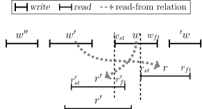
Figure 2: Old-new inversion. Two non-overlapping reads $r$ and $r^{\prime}$, both overlapping the write $w$, obtain out-of-order values. (Time goes from left to right.)

4 Quantifying the Atomicity Violations

In this section, we quantify the atomicity violations incurred in the 2AM algorithm. It follows from the correctness proof in Section 3.2 that the atomicity violations are exactly characterized by the “old-new inversions” in Case 2.2.2. Furthermore, the proof has also identified the necessary and sufficient condition for the “old-new inversions” phenomenon. We formally define it as follows.

Definition 3.

The old-new inversion involving a read $r$ consists of the read $r$, two writes $w$ and $w^{\prime}$, and a second read $r^{\prime}$, such that (see Figure 2)

1) $r_{st}\in[w_{st},w_{ft}]$, 2) $w^{\prime}$ immediately precedes $w$: $w^{\prime}\prec w$, and no other writes are between $w$ and $w^{\prime}$, 3) $r^{\prime}_{ft}\in[w_{st},r_{st}]$,

4) $r=R(w^{\prime})$, and 5) $r^{\prime}=R(w)$.

The five requirements for “old-new inversion” fall into two categories. The first three requirements involve the partial order $\prec$ on, and thus the concurrency patterns among, read/write operations. Intuitively, the higher degree of concurrency an execution shows, the more “old-new inversions” it may produce.

Definition 4.

The concurrency pattern involving a
read $r$ consists of the read $r$, two writes $w$ and $w^{\prime}$, and a second read $r^{\prime}$, such that

1. $r_{st}\in[w_{st},w_{ft}]$

2. $w^{\prime}$ immediately precedes $w$: $w^{\prime}\prec w$, and no other writes are between $w$ and $w^{\prime}$

3. $r^{\prime}_{ft}\in[w_{st},r_{st}]$

The concurrency pattern itself is not sufficient for old-new inversion. Only when the read/write semantics in the last two requirements of Definition 3 is also satisfied, does an old-new inversion arise. Thus, we define the read-write pattern conditioning on a concurrency pattern as follows.

Definition 5.

Given a concurrency pattern consisting of $r,r^{\prime},w,\textrm{and }w^{\prime}$, exactly as those in Definition 4, the read-write pattern requires

1. $r=R(w^{\prime})$

2. $r^{\prime}=R(w)$

In this way, an “old-new inversion” occurs if and only if the read-write pattern arises given that a corresponding concurrency pattern has emerged. A concurrency pattern may contain more than one such $r^{\prime}$ defined in Definition 4, as illustrated in Figure 2. Let $\mathrm{R^{\prime}}$ be a random variable denoting the number of $r^{\prime}$s in a concurrency pattern. Then, a read-write pattern arises if for some $r^{\prime}$, Definition 5 is satisfied. Therefore, the probability of “old-new inversions” conditioning on $\mathrm{R^{\prime}=m}$ ($m\geq 1$; $m$ can be as large as the number of all read operations) is the product of the probability of the concurrency patterns conditioning on $\mathrm{R^{\prime}=m}$ and the probability of the read-write patterns conditioning on $\mathrm{R^{\prime}=m}$. By the law of total probability, we obtain

$$\begin{split}\mathbb{P}&\{\text{violation of atomicity}\}=\mathbb{P}\{\mathrm{ONI}\}\\ &=\sum_{m\geq 1}\mathbb{P}\{\mathrm{ONI\mid R^{\prime}=m}\}\\ &=\sum_{m\geq 1}\mathbb{P}\{\mathrm{CP\mid R^{\prime}=m}\}\times\mathbb{P}\{\mathrm{RWP\mid R^{\prime}=m}\}.\end{split}$$ (4.1)

In the following two subsections, we propose a stochastic queueing model and a timed balls-into-bins model to analyze the concurrency pattern and read-write pattern in Equation (4.1), respectively. The frequently used notations and formulas are summarized in Table 1.

Table 1: Notations and formulas.

$N$: number of clients  $n$: number of replicas  $q\triangleq\lfloor n/2\rfloor+1$	Beta function: $B(x,y)=\int_{0}^{1}t^{x-1}(1-t)^{y-1}dt$
$\lambda$: issue/arrival rate of operations, $\mu$: service rate of operations	$r\triangleq\frac{(2\lambda+\mu)^{2}}{2(\mu+\lambda)^{2}},\quad s\triangleq\frac{1}{2}\frac{\mu}{\mu+\lambda},\quad p_{0}\triangleq\frac{1}{2}\left(1+(\frac{\lambda}{\mu+\lambda})^{2}\right)$
$\lambda_{r}$: rate for read latency, $\lambda_{w}$: rate for write latency, $\alpha=\frac{\lambda_{r}}{\lambda_{w}+\lambda_{r}}$	$t=\frac{1}{\lambda},\qquad t^{\prime}=\frac{2\lambda-\mu}{2\lambda\mu}$
$\begin{aligned} &J_{1}=\lambda_{r}\int_{0}^{t^{\prime}}e^{-\lambda_{r}(n-q+1)s}\left(1-e^{-\lambda_{r}s}\right)^{q-1}ds\\ &+\sum_{k=0}^{n-q}\frac{\binom{q-1}{k-1}\binom{n-q}{n-q-k}}{\binom{n}{n-q}}\lambda_{r}^{q}\,e^{\lambda_{w}t^{\prime}}\int_{t^{\prime}}^{\infty}e^{-(\lambda_{w}+\lambda_{r})s}\left(\frac{1-e^{-\lambda_{r}t^{\prime}}}{\lambda_{r}}+e^{\lambda_{w}t^{\prime}}\frac{e^{-(\lambda_{w}+\lambda_{r})t^{\prime}}-e^{-(\lambda_{w}+\lambda_{r})s}}{\lambda_{w}+\lambda_{r}}\right)^{k-1}\left(\frac{1-e^{-\lambda_{r}s}}{\lambda_{r}}\right)^{q-k}e^{-\lambda_{r}(n-q)s}ds\\ &+\sum_{k=0}^{n-q}\frac{\binom{q-1}{k}\binom{n-q}{n-q-k}}{\binom{n}{n-q}}\lambda_{r}^{q}\,\int_{t^{\prime}}^{\infty}e^{-\lambda_{r}s}\left(\frac{1-e^{-\lambda_{r}t^{\prime}}}{\lambda_{r}}+e^{\lambda_{w}t^{\prime}}\frac{e^{-(\lambda_{w}+\lambda_{r})t^{\prime}}-e^{-(\lambda_{w}+\lambda_{r})s}}{\lambda_{w}+\lambda_{r}}\right)^{k}\left(\frac{1-e^{-\lambda_{r}s}}{\lambda_{r}}\right)^{q-1-k}e^{-\lambda_{r}(n-q)s}ds.\end{aligned}$

4.1 Quantifying the Rate of Concurrency Patterns

To quantify the rate of concurrency patterns conditioning on $\mathrm{R^{\prime}=m}$, we need an analytical model of the workload consisting of one sequence of read/write operations from each client. For each client, the characteristics of its workload are captured by the rate of operations issued by it and the service time of each operation (i.e., $[o_{st},o_{ft}]$). We assume a Poisson process with parameter $\lambda$ for the former one and an exponential distribution with parameter $\mu$ for the latter one. The scenario of each client issuing a sequence of read/write operations is then encoded into a queueing model.

We thus consider $N$ independent, parallel $M/M/1$ queues (i.e., a single-server exponential queueing system), all with arrival rate $\lambda$ and service rate $\mu$ [24]. For each $M/M/1$ queue, we use the “first come first served” discipline and assume for simplicity that, if there is any operation in service, no more operations can enter it. The queue $Q_{0}$ represents the single writer.

To compute the probability that a concurrency pattern occurs in such a queueing system in the long run, we go through the following three steps.

Step 1: What is the stationary distribution for any two queues?

Let $X^{i}(t)$ be the number of operations in queue $i$ at time $t$. Then $X^{i}(t)$ is a continuous-time Markov chain with only two states: $0$ when the queue is empty and $1$ when some operation is being served. Its stationary distribution is:

$$P_{0} \triangleq P\left(X^{i}(\infty)=0\right)=\frac{\mu}{\mu+\lambda}$$

$$P_{1} \triangleq P\left(X^{i}(\infty)=1\right)=\frac{\lambda}{\mu+\lambda}$$

Let $Y(t)=\left(X^{i}(t),Y^{j}(t)\right)$ be the vector of the numbers of operations in queues $Q_{i}$ and $Q_{j}$. Since any two queues are independent, $Y(t)$ is a continuous-time Markov chain with four states $(0,0),(0,1),(1,0),\text{ and }(1,1)$. Its stationary distribution is:

$$P_{0,0}=\frac{\mu}{\mu+\lambda}\frac{\mu}{\mu+\lambda}=\frac{\mu^{2}}{(\mu+\lambda)^{2}}$$

$$P_{0,1}=P_{1,0}=\frac{\mu\lambda}{(\mu+\lambda)^{2}}\quad P_{1,1}=\frac{\lambda^{2}}{(\mu+\lambda)^{2}}$$

where,

$$P_{i,j}\triangleq P\left(Y\left(\infty\right)=\left(i,j\right)\right)\qquad i,j\in\{0,1\}.$$

Step 2: Given a read $r$ in $Q_{i}$, what is the probability of the event, denoted $E$, that it starts during the service period of some write $w$ in $Q_{0}$ (formally, $r_{st}\in[w_{st},w_{ft}]$ in Definition 4)?

The probability of $E$ equals the probability that when $r$ arrives at $Q_{i}$, it finds $Q_{i}$ empty (denoted $E_{i}$) and as a bystander $Q_{0}$ full (denoted $E_{0}$). Since events $E_{i}$ and $E_{0}$ are independent, we have

$$P(E) =P(E_{i}\land E_{0})=P(E_{i})\cdot P(E_{0})$$

$$=P_{0}\cdot P_{1}\qquad{\text{(by the PASTA property}\cite[cite]{[\@@bibref{}{Ross10}{}{}]})}$$

$$=\frac{\mu\lambda}{(\mu+\lambda)^{2}}$$

Step 3: Conditioning on Step 2, what is the probability of the event, denoted $E_{N-1,m}$, that there are totally $m$ read operations (denoted $r^{\prime}$) in $N-1$ queues (besides $Q_{0}$) which finish during the time period $[w_{st},r_{st}]$ (formally, $r^{\prime}_{ft}\in[w_{st},r_{st}]$ in Definition 4)?

First, the length $L=r_{st}-w_{st}$ of the time period $[w_{st},r_{st}]$ is exactly the inter-arrival time of $Q_{i}$, which is exponential with rate $\lambda$.

The calculations in Appendix A yield

$$\mathbb{P} \{\mathrm{CP\mid R^{\prime}=m}\}=\mathbb{P}(E_{N-1,m})$$

$$=\sum_{k=0}^{N-2}\binom{N-1}{k}\binom{m-1}{N-k-2}p_{0}^{k}r^{N-k-1}s^{m},$$ (4.2)

when $m\geq 1$. For the special case $m=0$, we have

$$\mathbb{P}\{\mathrm{CP\mid R^{\prime}=0}\}=\mathbb{P}(E_{N-1,0})=p_{0}^{N-1}.$$

Summing over $m$ ($m\geq 1$), we also get the probability that there exists a concurrency pattern (for some read $r$):

$$\mathbb{P}\{\mathrm{CP}\}=1-\mathbb{P}\{\mathrm{CP\mid R^{\prime}=0}\}=1-p_{0}^{N-1}$$ (4.3)

4.2 Quantifying the Rate of Read-Write Patterns

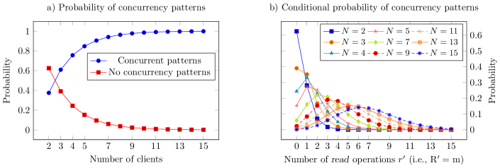
Figure 3: The probability of concurrency patterns: a) with vs. without concurrency patterns; b) conditioning on $\mathrm{R^{\prime}=m}$ ($\lambda=10s^{-1},\mu=10s^{-1}$).

Given the concurrency patterns, we further quantify the rate of read-write patterns conditioning on $\mathrm{R^{\prime}=m}$:

$$r=R(w^{\prime})\land\exists r^{\prime}:r^{\prime}=R(w)$$

where $r^{\prime}$ is among the $m$ read operations in Step 3 in Section 4.1. To this end, we shall explore in detail the majority quorum systems used in the 2AM algorithm. We assume that 1) no node failure or link failure occurs; and 2) to complete an operation (read or write), the client accesses all the $n$ replicas and wait for the first $q\triangleq\lfloor n/2\rfloor+1$ acknowledgments from them. It follows that:

$$\mathbb{P} \{\mathrm{RWP\mid R^{\prime}=m}\}$$

$$=\mathbb{P}\{r=R(w^{\prime})\land\exists r^{\prime}:r^{\prime}=R(w)\}$$

$$\leq\mathbb{P}\{r\neq R(w)\land\exists r^{\prime}:r^{\prime}=R(w)\}$$

$$=\mathbb{P}\{r\neq R(w)\}\times\mathbb{P}\{\exists r^{\prime}:r^{\prime}=R(w)\mid r\neq R(w)\}$$ (4.4)

$$=\mathbb{P}\{r\neq R(w)\}\times\Big{(}1-\mathbb{P}\{r^{\prime}\neq R(w)\mid r\neq R(w)\}^{m}\Big{)}$$

where $r\neq R(w)$ (resp. $r^{\prime}\neq R(w)$) denotes that $r$ (resp. $r^{\prime}$) does not read from $w$. The inequality is due to the fact that $r=R(w^{\prime})$ implies $r\neq R(w)$. We then focus on the calculations of $\mathbb{P}\{r\neq R(w)\}$ and $\mathbb{P}\{r^{\prime}\neq R(w)\mid r\neq R(w)\}$.

Which write would be read from by some read depends on the states of the replicas from which it collects the first $\lfloor n/2\rfloor+1$ acknowledgments. The states of the replicas further depend on the timing issues in the 2AM algorithm, such as message delays and the time lag between the events that the messages are sent. Taking into account the timing issues, we propose the timed balls-into-bins model for the read and write procedures in the 2AM algorithm. Let $D_{r}$ (resp. $D_{w}$) be a (non-negative) continuous random variable denoting the message delay for read (resp. write) operations during a communication round-trip. Let $T$ be a (non-negative) continuous random variable denoting the time lag between the time when two messages of interest are sent, and $t$ a realization (or called an observed value) of $T$.

In the timed balls-into-bins model, there are $n$ bins (corresponding to $n$ replicas). Consider two robots $R_{1}$ and $R_{2}$ (corresponding to read or write operations) which can produce multiple balls (corresponding to messages) instantaneously. At time 0, robot $R_{1}$ 1) produces $n$ balls instantaneously; 2) Immediately these $n$ balls are independently sent to the $n$ bins, one ball per bin; 3) The delays for the balls going from the robot to its destination bin are independent and identically distributed with the same distribution as $D_{r}$ or $D_{w}$ as defined above, depending on whether the robot represents a read or a write.

At time $t$ (defined above), robot $R_{2}$ independently does exactly the same thing as robot $R_{1}$ does (i.e., 1), 2), and 3) for robot $R_{1}$ above).

Each probability to calculate is related to an event in an instantiation of the timed balls-into-bins model.

To calculate $\mathbb{P}\{r\neq R(w)\}$, we are concerned with the model in which the robots $R_{1}$ and $R_{2}$ represent the write operation $w^{\prime}$ and the read operation $r$ involved in an “old-new inversion”, respectively. Furthermore, we assume that the random variable $D_{r}$ (resp. $D_{w}$) for time delay is exponentially distributed with rate $\lambda_{r}$ (resp. $\lambda_{w}$). The time lag $T$ between the events that $w^{\prime}$ and $r$ are issued (meanwhile messages are sent to replicas) corresponds to the time period $[w_{st},r_{st}]$. That is to say, $T$ is an exponential random variable with rate $\lambda$, as shown in Section 4.1 (See Step 3). For simplicity, we take the time lag $t$ to be the expectation of $T$, i.e., $t=\frac{1}{\lambda}$. Finally, we are interested in the time point $t^{\prime}$ when exactly $q\triangleq\lfloor n/2\rfloor+1$) of the $n$ bins have received the balls from $R_{2}$ (i.e., $r$), and denote the set of these $\lfloor n/2\rfloor+1$ bins by $B$. In terms of the timed balls-into-bins model, the case of $r\neq R(w)$ corresponds to the event $E$ that none of the $q\triangleq\lfloor n/2\rfloor+1$ bins in $B$ receives a ball from $R_{1}$ (i.e., $w$) before it receives a ball from $R_{2}$ (i.e., $r$).

The calculations in Appendix B.1 yield

$$\mathbb{P}\{r\neq R(w)\}=e^{-q\lambda_{w}t}\frac{\alpha^{q}B\left(q,\alpha(n-q)+1\right)}{B\left(q,n-q+1\right)},$$ (4.5)

where $\alpha=\frac{\lambda_{r}}{\lambda_{w}+\lambda_{r}}$ and $B$ denotes the Beta function.

To calculate $\mathbb{P}\{r^{\prime}\neq R(w)\mid r\neq R(w^{\prime})\}$, we introduce a slightly generalized timed balls-into-bins model. In the new model, robot $R_{2}$ picks $p$ ($0<p\leq n$) bins uniformly at random (without replacement) and sends a ball to each of them (see Appendix B.2). The calculations in Appendix B.3 yield

$$\mathbb{P}\{r^{\prime}\neq R(w)\mid r\neq R(w)\}=\left\{\begin{array}[]{ll}\frac{J_{1}}{B(q,n-q+1)}&\textrm{if }n>2,\\ 1&\textrm{if }n=2.\end{array}\right.$$ (4.8)

Substituting Equations (4.5) and (4.8) into Equation (4.2) gives, for $n>2$, the rate of read-write patterns conditioning on $\mathrm{R^{\prime}=m}$:

$$\mathbb{P} \{\mathrm{RWP\mid R^{\prime}=m}\}$$

$$\leq\mathbb{P}\{r\neq R(w)\}\times\Big{(}1-\mathbb{P}\{r^{\prime}\neq R(w)\mid r\neq R(w)\}^{m}\Big{)}$$

$$\leq e^{-q\lambda_{w}t}\frac{\alpha^{q}B\left(q,\alpha(n-q)+1\right)}{B\left(q,n-q+1\right)}$$

$$\quad\cdot\left(1-\left(\frac{J_{1}}{B(q,n-q+1)}\right)^{m}\right).$$ (4.9)

For $n=2$, we have

$$\mathbb{P}\{\mathrm{RWP\mid R^{\prime}=m}\}=0.$$

Notice that $\mathbb{P}\{\mathrm{RWP\mid R^{\prime}=0}\}=0$ since there are no concurrency patterns at all.

4.3 Numerical Results and Discussions

In light of the complicated analytical formulation, we present the numerical results on concurrency patterns, read-write patterns, and old-new inversions. The numerical results have not only demonstrated that “old-new inversions” (and thus, atomicity violations) rarely occur as expected, but also clearly revealed that the read-write patterns dominate in guaranteeing such rare violations.

Figure 3 presents the probability of concurrency patterns, given $\lambda=10s^{-1}\textrm{ and }\mu=10s^{-1}$, meaning that the expected arrival rate is 10 operations per second and the expected service time is 100 ms. First of all, Figure 3a) shows that the probability of concurrency pattern is quite high, and it rapidly increases with the number of clients. For example when $N=15$, it nearly reaches $1$: intuitively, for each read $r$, there almost always exist concurrency patterns involving it. Figure 3b) further explores the probability of concurrency patterns conditioning on the number $m$ of reads $r^{\prime}$ (i.e., $\mathbb{P}\{\mathrm{CP\mid R^{\prime}=m}\}$). Here $m=0$ indicates that there are no concurrency patterns at all, corresponding to the (square-marked) line at the bottom in Figure 3a). One key observation from Figure 3b) is that the conditional probability of concurrency patterns concentrates on the small values of $m$’s, and for each $N$ the value of $m$ which achieves the maximum is smaller than $N$. This observation partly justifies the assumption made in the model for calculating $\mathbb{P}\{r^{\prime}\neq R(w)\mid r\neq R(w)\}$ (see Appendix B.2) that there is at most one such $r^{\prime}$ in a single (client) process.

Figure 4, as well as Table 2, presents the probability of read-write patterns, given $\lambda=10s^{-1},\mu=10s^{-1},\textrm{and }\lambda_{r}=\lambda{w}=20s^{-1}$. The latter two parameters mean that the expected message delay is 50 ms. According to Equation (4.2), we distinguish the probability $\mathbb{P}\{r\neq R(w)\}$ from another one $1-\mathbb{P}\{r^{\prime}\neq R(w)\mid r\neq R(w)\}^{m}$ (in Figure 4, we take the extreme value of $m=1$), and observe that the former dominates in keeping the probability of read-write patterns quite low. The observation that $\mathbb{P}\{r\neq R(w)\}$ is quite low has demonstrated the effectiveness of the majority quorum system used in the 2AM algorithm, under which a read would, with a high probability, not miss a concurrent write that starts earlier. In addition, if a read $r$ has happened to miss such a concurrent write, it is still quite likely to avoid an old-new inversion: $r$ can reasonably infer, from the low values of $1-\mathbb{P}\{r^{\prime}\neq R(w)\mid r\neq R(w)\}$, that the preceding reads $r^{\prime}$ would not have read from that write either.

Table 2: Numerical results on the probabilities of $\{r\neq R(w)\}$ and $1-\{r^{\prime}\neq R(w)\mid r\neq R(w)\}$.

# replicas	$\mathbb{P}\{r\neq R(w)\}$	$1-\mathbb{P}\{r^{\prime}\neq R(w)$ $\mid r\neq R(w)\}$	# replicas	$\mathbb{P}\{r\neq R(w)\}$	$1-\mathbb{P}\{r^{\prime}\neq R(w)$ $\mid r\neq R(w)\}$
$2$	$0.00457891$	$1.0$	$9$	$8.51249\times 10^{-6}$	$0.0243758$
$3$	$0.00732626$	$0.0409628$	$10$	$7.20025\times 10^{-7}$	$0.0353241$
$4$	$0.000566572$	$0.0561367$	$11$	$8.89660\times 10^{-7}$	$0.0203645$
$5$	$0.00077461$	$0.0356626$	$12$	$7.60436\times 10^{-8}$	$0.0294186$
$6$	$0.0000628992$	$0.0511399$	$13$	$9.28973\times 10^{-8}$	$0.0171705$
$7$	$0.0000813243$	$0.0294467$	$14$	$8.00055\times 10^{-9}$	$0.0246974$
$8$	$6.77295\times 10^{-6}$	$0.0426608$	$15$	$9.69478\times 10^{-9}$	$0.0145951$

Table 3: Numerical results on the probabilities of concurrency patterns, read-write patterns, and old-new inversions.

# replicas	$\mathbb{P}\{\mathrm{CP}\}$	$\mathbb{P}\{\mathrm{RWP}\mid\mathrm{CP}\}$	$\mathbb{P}\{\mathrm{ONI}\}$	# replicas	$\mathbb{P}\{\mathrm{CP}\}$	$\mathbb{P}\{\mathrm{RWP}\mid\mathrm{CP}\}$	$\mathbb{P}\{\mathrm{ONI}\}$
$2$	$0.28125$	$0.$	$0.$	$9$	$0.9447$	$7.06025\times 10^{-6}$	$7.30744\times 10^{-7}$
$3$	$0.518555$	$0.00088802$	$0.000203683$	$10$	$0.95874$	$1.04312\times 10^{-6}$	$9.93356\times 10^{-8}$
$4$	$0.677307$	$0.000183791$	$0.0000352958$	$11$	$0.968604$	$9.37995\times 10^{-7}$	$8.16935\times 10^{-8}$
$5$	$0.781222$	$0.000266569$	$0.0000437181$	$12$	$0.975675$	$1.34085\times 10^{-7}$	$1.08822\times 10^{-8}$
$6$	$0.849318$	$0.0000450835$	$6.49226\times 10^{-6}$	$13$	$0.98085$	$1.16911\times 10^{-7}$	$8.77158\times 10^{-9}$
$7$	$0.89429$	$0.0000478926$	$6.08721\times 10^{-6}$	$14$	$0.984717$	$1.63195\times 10^{-8}$	$1.15178\times 10^{-9}$
$8$	$0.924335$	$7.43561\times 10^{-6}$	$8.53810\times 10^{-7}$	$15$	$0.987662$	$1.39573\times 10^{-8}$	$9.18283\times 10^{-10}$

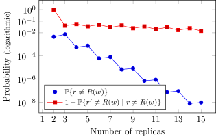
Figure 4: The probability of read-write patterns ($\lambda=10s^{-1},\mu=10s^{-1},\lambda_{r}=\lambda{w}=20s^{-1}$).

Substituting Equations (4.1) and  (4.2) into Equation (4.1), we obtain the rate of violating atomicity:

$$\mathbb{P} \{\text{violation of atomicity}\}=\mathbb{P}\{\mathrm{ONI}\}$$

$$=\sum_{m\geq 1}\mathbb{P}\{\mathrm{CP\mid R^{\prime}=m}\}\times\mathbb{P}\{\mathrm{RWP\mid R^{\prime}=m}\}$$

$$\approx\left(\sum_{k=0}^{N-2}\binom{N-1}{k}\binom{m-1}{N-k-2}p_{0}^{k}r^{N-k-1}s^{m}\right)$$

$$\quad\cdot e^{-q\lambda_{w}t}\frac{\alpha^{q}B\left(q,\alpha(n-q)+1\right)}{B\left(q,n-q+1\right)}$$

$$\quad\cdot\left(1-\left(\frac{J_{1}}{B(q,n-q+1)}\right)^{m}\right).$$ (4.10)

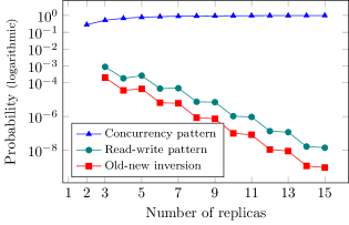
Figure 5: The probabilities of concurrency patterns, read-write patterns, and old-new inversions ($\lambda=10s^{-1},\mu=10s^{-1},\lambda_{r}=\lambda{w}=20s^{-1},N=n$).

Notice that Equation (4.3) is an approximation since the timed balls-into-bins model used for calculating the probability of read-write patterns (specifically, for the case of $\{r^{\prime}\neq R(w)\mid r\neq R(w)\}$ in Appendix B.2) assumes that there is at most one such $r^{\prime}$ in a single process, while the model for calculating the probability of concurrency patterns does not.

Figure 5, as well as Table 3, presents the probability of old-new inversions according to Equation (4.3) with $N=n$. We also list the probabilities of concurrency patterns and read-write patterns, which are calculated as follows:

$$\mathbb{P}\{\mathrm{CP}\} =\sum_{m=1}^{N-1}\mathbb{P}\{\mathrm{CP}\mid\mathrm{R^{\prime}=m}\}$$

$$\mathbb{P}\{\mathrm{RWP}\mid\mathrm{CP}\} =\sum_{m=1}^{N-1}\mathbb{P}\{\mathrm{RWP}\mid\mathrm{R^{\prime}=m}\}.$$

Based on Figure 5 and Table 3, we first observe that the probability of old-new inversions (and thus, atomicity violations) is sufficiently small, demonstrating that 2-atomicity and the 2AM algorithm is “good enough” in distributed storage systems. More importantly, it also reveals that the read-write patterns dominate in guaranteeing such rare violations, compared to the concurrency patterns which occur quite often.

Notice that the principles underlying our theoretical analysis (as well as the numerical analysis) have been decoupled from the assumptions we adopt about the networks and workloads. These principles mainly consist of the introduction to old-new inversion, the decomposition of it into concurrency pattern and read-write pattern, the queueing model for analyzing concurrency patterns, and the timed balls-into-bins model for analyzing read-write patterns. Network conditions and workload types may vary in different scenarios. However, the principles and the methodology of our analysis still apply.

5 Experiments and Evaluations

In this section, we empirically study the 2AM algorithm. To this end, we have implemented a prototype data storage system among mobile phones, which provides 2-atomic data access based on the 2AM algorithm and atomic data access based on the ABD algorithm. We compare the read latency in both algorithms. We also measure the proportion of atomicity violations incurred in the 2AM algorithm.

5.1 Experimental Design

Our prototype system comprises a collection of Google Nexus5 smartphones (CPU: Qualcomm Snapdragon™ 800, 2.26GHz, Memory: 16GB, Android: 4.4.2), equipped with 72Mbps wireless LAN. In both algorithms, each phone acts as both a client and a server replica. As a client, it collects its own execution trace for offline analysis. Clocks on the phones are synchronized with the same desktop computer.

We explore three kinds of parameters: 1) algorithm parameters: replication factor (i.e., the number of phones) and consistency levels (i.e., atomicity or 2-atomicity); 2) workload parameters: the number of read/write operations issued by each client and the issue rate on each client; and 3) network parameter: the injected random delay in network communication, modeling the various degrees of asynchrony.

We are concerned with two metrics:

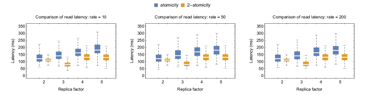
Figure 6: Comparison of read latency in both the ABD atomicity algorithm and the 2AM algorithm.

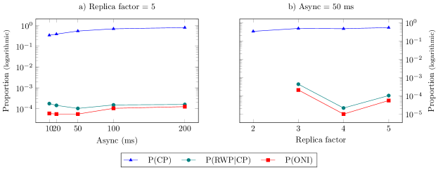
Figure 7: The proportions of concurrency patterns $\mathrm{P(CP)}$, read-write patterns among concurrency patterns $\mathrm{P(RWP|CP)}$, and “old-new inversions” $\mathrm{P(ONI)}$. ($\log 0$ is not defined and thus not shown.)

Latency: We compare the read latency in both algorithms by varying the replication factors and the issue rates of operations in the workload. Each client issues reads/writes at a Poisson rate $\lambda$ (= 5, 10, 20, 50, 100, or 200) per second. For each $\lambda$, the replication factors vary from 2 to 5. Each reader issues 50, 000 read operations. The single writer issues only write operations. In addition, the size of the keyspace is fixed to 1. The key takes integer values from 0 to 4.

Violations of atomicity: We quantify the violations of atomicity incurred in the 2AM algorithm by varying the replication factors and the network delays. The replication factors vary from 2 to 5. For each replication factor, the injected random delays in network communication are uniformly distributed over integers in $[0,r)$ ($r$ can be 10, 20, 50, 100, and 200 ms). Each client issues 200, 000 operations. The single writer issues only write operations. On each client, operations arrive at a Poisson rate of 50 per second so that the system operates at its full capacity. The size of the keyspace is 1 and the “hotspot” key takes integer values from 0 to 4.

5.2 Experimental Result 1: Latency

We visualize the latency data using box plots (Figure 6), where the box indicates the median and the 25th and 75th percentile scores, while the whiskers indicate variability outside the lower and upper quartiles. The medians are marked by the white lines between boxes. The outliers (probably due to the garbage collection in phones) are not shown.

As indicated in Figure 6, the read latency is significantly reduced using the 2AM algorithm which completes each read in one round-trip. In the case of 5 replicas, the reduction of the latency is about 29%.

Figure 6 also shows that the issue rate of operations on each client has little impact on the read latency. This is due to the fact that in both algorithms, reads or writes proceed independently, especially without waiting for each other (the cases of “rate = 5”, “rate = 20”, and “rate = 100” are thus not shown). On the other hand, the more the replicas are involved, the higher the read latency is incurred. This is because each read needs to contact all the replicas and waits for acknowledgments from a majority of them.

5.3 Experimental Result 2: Atomicity Violations

To measure the proportion of the atomicity violations incurred in the 2AM algorithm, we count the number of read operations ($\mathrm{\#R}$) and the occurrences of concurrency patterns ($\mathrm{\#CP}$) and read-write patterns ($\mathrm{\#RWP}$). Because each concurrency pattern or each read-write pattern is associated with some read operation $r$, we are concerned with the following quantities:

$$\mathrm{P(CP)=\frac{\#CP}{\#R}},\mathrm{P(RWP|CP)=\frac{\#RWP}{\#CP}},\mathrm{P(ONI)=\frac{\#RWP}{\#R}}$$

In this manner, the proportion of “old-new inversions” (and thus the violations of atomicity) $\mathrm{P(ONI)}$ equals the product of $\mathrm{P(CP)}$ and $\mathrm{P(RWP|CP)}$:

$$\mathrm{P(ONI)}=\mathrm{P(CP)}\cdot\mathrm{P(RWP|CP)}.$$ (5.1)

Notice that this is not the case in theory, according to Equation (4.1). Therefore, Equation (5.1) is a practical approximation to Equation (4.1) in theory, without going into the details of conditioning on $\mathrm{R^{\prime}=m}$. The feasibility of such an approximation will be justified by the experimental results presented shortly, in the sense that the key observations drawn from the numerical results based on the equations in theory fit well with the empirical data and Equation (5.1).

Table 4: The numbers and proportions of concurrency patterns and read-write patterns (replication factor = 5).

# async (ms)	# read operations	# concurrency patterns	# read-write patterns	P(CP)	P(RWP${\bf\mid}$CP)	P(ONI)
$10$	$800,000$	$269,061$	$47$	$0.336326$	$0.000174682$	$0.00005875$
$20$	$800,000$	$306,274$	$44$	$0.382843$	$0.000143662$	$0.000055$
$50$	$800,000$	$428,344$	$44$	$0.53543$	$0.000102721$	$0.000055$
$100$	$800,000$	$549,102$	$83$	$0.686378$	$0.000151156$	$0.00010375$
$200$	$800,000$	$627,814$	$100$	$0.784768$	$0.000159283$	$0.000125$

Table 5: The numbers and proportions of concurrency patterns and read-write patterns (async = 50 ms).

# replicas	# read operations	# concurrency patterns	# read-write patterns	P(CP)	P(RWP${\bf\mid}$CP)	P(ONI)
$2$	$200,000$	$66,985$	$0$	$0.334925$	$0$	$0$
$3$	$400,000$	$192,902$	$83$	$0.482255$	$0.00043027$	$0.0002075$
$4$	$600,000$	$280,091$	$6$	$0.466818$	$0.0000214216$	$0.00001$
$5$	$800,000$	$428,344$	$44$	$0.53543$	$0.000102721$	$0.000055$

Due to the limited space, Tables 4 and 5 summarize part of the experimental results (also shown in Figure 7). In Table 4, the replication factor is 5 (thus the number of read operations is 800, 000) and the parameter of async varies from 10 ms to 200 ms. In Table 5, the parameter of async is 50 ms and the replication factors vary from 2 to 5. As shown in Table 4, the higher the degree of asynchrony is, the more concurrency patterns there are. On the other hand, the number of occurrences of concurrency patterns grows as the replication factor increases (Table 5). Accordingly, the proportion of concurrency patterns $\mathrm{P(CP)}$ also increases along with the replication factor, as implied by Equation (4.3).

For the number of read-write patterns, the experimental results exhibit three features. First, no read-write patterns (and thus no “old-new inversions”) arise in only 2 replicas. This is because both read and write operations are required to contact both replicas to complete. Second, there are fewer read-write patterns in the case of 4 replicas than those in the case of 3 or 5 replicas. In the case of 4 replicas, each read contacts 3 replicas according to the mechanism of the majority quorum system, accounting for 75% of them, and gains more opportunities to obtain the latest data version. For 3 or 5 replicas, the majorities account for 66.7% and 60%, respectively. (Notice that the majority accounts for 100% in the case of 2 replicas.) Third, Table 4 shows that the degree of asynchrony also contributes to the occurrences of read-write patterns since it may lead to out-of-order message delivery in the timed balls-into-bins model (Section 4.2).

One of the most important observations concerning these experiments is that they have confirmed our theoretical analysis in Section 4.3. First, the proportion of “old-new inversions” $\mathrm{P(ONI)}$ is quite small (less than 0.1‰ in most executions), demonstrating that 2-atomicity is “good enough” in data storage systems regarding the violations of atomicity. More importantly, the proportion of read-write patterns among concurrency patterns $\mathrm{P(RWP|CP)}$ is much less than that of concurrency patterns $\mathrm{P(CP)}$ themselves. Namely, although concurrency patterns appear frequently (e.g., accounting for more than $50\%$ in the setting of 5 replicas and 50 ms async), only a quite small portion of them satisfy the read-write semantics of read-write pattern (Definition 5) to constitute the “old-new inversions” (e.g., about 0.1‰ in the same setting). It follows that the read-write patterns dominate in guaranteeing such rare atomicity violations incurred in the 2AM algorithm.

In conclusion, the experimental results (which have confirmed the theoretical analysis) show that 2-atomicity and the 2AM algorithm are “good enough” in distributed storage systems, by achieving low latency, bounded staleness, and rare atomicity violations.

6 Related Work

We divide the related work into three categories: consistency/latency tradeoff, complexity of emulating atomic registers, and quantifying weak consistency.

Consistency/latency tradeoff. Designing distributed storage systems involve a range of tradeoffs among, for instance, consistency, latency, availability, and fault-tolerance. The well-known CAP theorem [11] states that it is impossible for any distributed data storage system to achieve consistency, availability, and network-partition tolerance simultaneously. More recently, another tradeoff — between consistency and latency — has been considered more influential on the designs of distributed storage systems, as it is present at all times during system operation [4].

In this paper we study the consistency/latency tradeoff and propose the notion of almost strong consistency as a better balance option for it.

Complexity of emulating atomic registers. The ABD algorithm for atomicity [7] [6] emulates the atomic, single-writer multi-reader registers in unreliable, asynchronous networks, given that a minority of nodes may fail. It requires each read to complete in two round-trips. Dutta et al. [16] proved that it is impossible to obtain a fast emulation, where both reads and writes complete in one round-trip (i.e., low latency in our terms). Georgiou et al. [17] studied the semi-fast emulations (of atomic, single-writer multi-reader registers) where most reads complete in one round-trip. Guerraoui et al. considered the best-cases complexity, assuming synchrony, no or few failures, and absence of read/write contention. In this situation, fast emulations do exist [18].

We investigate the notion of almost strong consistency in terms of 2-atomicity, namely, to emulate 2-atomic, single-writer multi-reader registers. Our 2AM algorithm completes both reads and writes in one round-trip.

Quantifying weak consistency. Weak consistency can be quantified from four perspectives: data versions, randomness, timeliness, and numerical values. Modern distributed storage systems often settle for weak consistency and allow reads to obtain data of stale versions [15], [14]. The semantics of $k$-atomicity [5] guarantees that the data returned is of a bounded staleness. Without guarantee of bounded staleness, random registers [22] provide a probability distribution over the set of out-of-date values that may be returned. Using PBS (Probabilistically Bounded Staleness) [9], one can obtain the probability of reading one of the latest $k$ versions of a data item. Timed consistency models [25] require writes to be globally visible within a period of time. PBS [9] also calculates the probability of reading a write $t$ seconds after it returns. TACT [26], a continuous consistency model, integrates the metric on numerical error with staleness.

The 2-atomicity (and almost strong consistency) semantics integrates bounded staleness of versions with randomness. Our 2AM algorithm completes each read in one round-trip, in contrast to that of $k$-atomicity [5]. It differs from random registers [22] and PBS [9] in two aspects: First, it provides guarantee of deterministically bounded staleness. Second, the rate of violations is quantified with respect to atomicity instead of regularity (as in [22] and [9]), which is more challenging since we shall deal with concurrent operations. To do this, we propose a stochastic queueing model for analyzing the concurrency pattern first and then a timed balls-into-bins model for analyzing the read-write pattern.

7 Conclusion and Future Work

In this paper we propose the notion of almost strong consistency as a better balance option for the consistency/latency tradeoff. It provides both deterministically bounded staleness of data versions for each read and probabilistic quantification on the rate of “reading stale values”, while achieving low latency. In the context of distributed storage systems, we investigate almost strong consistency in terms of 2-atomicity. Our 2AM (2-Atomicity Maintenance) algorithm completes both reads and writes in one communication round-trip, and guarantees that each read obtains the value of within the latest 2 versions. We also quantify the rate of atomicity violations incurred in the 2AM algorithm, both analytically and experimentally.

We identify three problems for future work. First, it is worthwhile to conduct more intensive simulations or experiments, in order to reveal the key parameters and guiding principles for distributed storage system design. Second, we plan to study 2-atomic, multi-writer multi-reader registers. One key problem is whether they admit implementations which complete both reads and writes in one round-trip. Finally, we hope to extend the notion of almost strong consistency from shared registers to snapshot objects.

8 Acknowledgments

This work is supported by the National 973 Program of China (2015CB352202) and the National Science Foundation of China (61272047, 91318301, 61321491). The authors thank the users from MathOverflow [1] [2] for helpful discussions on the calculations in Section 4.

Appendix A Calculations of $\boldsymbol{\mathbb{P}(E_{N-1,m})}$ in Section 4.1

In this section, we compute the probability of the event, denoted $E_{N-1,m}$, that there are totally $m$ read operations in $N-1$ queues (besides $Q_{0}$) which finish during the time period $[w_{st},r_{st}]$ (Step 3 in Section 4.1).

We first consider a single queue. Let $D$ be a random variable denoting the number of operations in one particular queue which finish during the time period $r_{st}-w_{st}$. Its probability distribution $\mathbb{P}(D=d)$ is given in Appendix A.1. Then, we take into account all the $N-1$ ($N>1$) queues, besides $Q_{0}$. The calculations of $\mathbb{P}(E_{N-1,m})$ are given in Appendix A.2.

A.1 Calculations of $\boldsymbol{\mathbb{P}(D=d)}$

Let $D$ be a random variable denoting the number of operations in one particular queue which finish during the time period $L=r_{st}-w_{st}$. To compute its probability distribution, we condition on whether $w$ sees this queue as empty (denoted as an event $E_{\emptyset}$) or not (denoted as an event $E_{\neq\emptyset}$).

1) If it sees this queue empty (with probability $a_{0}=\frac{\mu}{\mu+\lambda}$), then the number of departures, during the time period $r_{st}-w_{st}$, has the conditional distribution:

$$\mathbb{P} (D=d\mid E_{\emptyset})$$

$$=\left\{\begin{array}[]{ll}\mathbb{P}(L<A_{0}+S_{0})&\textrm{if $d=0$}\\ \\ \mathbb{P}\big{(}\smashoperator[r]{\sum_{i=1}^{d}}(A_{i}+S_{i})\leq L<\sum_{i=1}^{d+1}(A_{i}+S_{i})\big{)}&\textrm{if $d\geq 1$}\end{array}\right.$$

$$=\left\{\begin{array}[]{ll}\frac{2\lambda+\mu}{2(\lambda+\mu)}&\textrm{if $d=0$}\\ \\ (1-\frac{1}{2}\frac{\mu}{\mu+\lambda})(\frac{1}{2}\frac{\mu}{\mu+\lambda})^{d}&\textrm{if $d\geq 1$}\end{array}\right.$$

where $A_{i}$ are independent and identically distributed (iid) exponential random variables with parameter $\lambda$ corresponding to the inter-arrival times of operations in the other queue, and $S_{i}$ are iid exponential random variables with parameter $\mu$ corresponding to the service time of these operations.

Here we briefly demonstrate the calculation of

$$\mathbb{P}\big{(}\smashoperator[r]{\sum_{i=1}^{d}}(A_{i}+S_{i})\leq L<\sum_{i=1}^{d+1}(A_{i}+S_{i})\big{)}\quad(\textrm{when }d\geq 1).$$

For convenience, we write

$$R_{d}\triangleq\smashoperator[r]{\sum_{i=1}^{d}}(A_{i}+S_{i})\textrm{ and }R_{d+1}\triangleq\sum_{i=1}^{d+1}(A_{i}+S_{i}).$$

As $L$ is an exponential random variable with parameter $\lambda$ and is independent of $R_{d}$, we have

$$\mathbb{P}(R_{d}\leq L)=\int P(L\geq x)dP_{R_{d}}(x)=\mathbb{E}(e^{-\lambda R_{d}}).$$

It follows from the independence assumptions that,

$$\mathbb{P} (R_{d}\leq L<R_{d+1})=\mathbb{E}(e^{-\lambda R_{d}}-e^{-\lambda R_{d+1}})$$

$$=\prod_{i=1}^{d}\mathbb{E}(e^{-\lambda(A_{i}+S_{i})})-\prod_{i=1}^{d+1}\mathbb{E}(e^{-\lambda(A_{i}+S_{i})})$$

$$=\big{(}\mathbb{E}(e^{-\lambda(A_{1}+S_{1})})\big{)}^{d}-\big{(}\mathbb{E}(e^{-\lambda(A_{1}+S_{1})})\big{)}^{d+1}$$

$$=(\frac{1}{2}\frac{\mu}{\mu+\lambda})^{d}-(\frac{1}{2}\frac{\mu}{\mu+\lambda})^{d+1}$$

$$=(1-\frac{1}{2}\frac{\mu}{\mu+\lambda})(\frac{1}{2}\frac{\mu}{\mu+\lambda})^{d}$$

2) Similarly, if it sees this queue full (with probability $a_{1}=\frac{\lambda}{\mu+\lambda}$), we have

$$\mathbb{P} (D=d\mid E_{\neq\emptyset})$$

$$=\left\{\begin{array}[]{ll}\mathbb{P}(L<S_{0})&\textrm{if $d=0$}\\ \\ \mathbb{P}\big{(}\smashoperator[r]{\sum_{i=1}^{d}}S_{i}+\sum_{i=1}^{d-1}A_{i}\leq L\\ \qquad\qquad<\smashoperator[r]{\sum_{i=1}^{d+1}}S_{i}+\sum_{i=1}^{d}A_{i}\big{)}&\textrm{if $d\geq 1$}\end{array}\right.$$

$$=\left\{\begin{array}[]{ll}\frac{\lambda}{\mu+\lambda}&\textrm{if $d=0$}\\ \\ \frac{\mu+2\lambda}{\mu+\lambda}(\frac{1}{2}\frac{\mu}{\mu+\lambda})^{d}&\textrm{if $d\geq 1$}\end{array}\right.$$

Using the law of total probability, we obtain

$$\mathbb{P} (D=d)$$

$$=\frac{\mu}{\mu+\lambda}\mathbb{P}(D=d\mid E_{\emptyset})+\frac{\lambda}{\mu+\lambda}\mathbb{P}(D=d\mid E_{\neq\emptyset})$$

$$=\left\{\begin{array}[]{ll}\frac{1}{2}\big{(}1+(\frac{\lambda}{\mu+\lambda})^{2}\big{)}&\textrm{if $d=0$}\\ \\ \frac{(2\lambda+\mu)^{2}}{2(\mu+\lambda)^{2}}(\frac{1}{2}\frac{\mu}{\mu+\lambda})^{d}&\textrm{if $d\geq 1$}\end{array}\right.$$ (A.4)

A.2 Calculations of $\boldsymbol{\mathbb{P}(E_{N-1,m})}$

Taking into account all the $N-1$ ($N>1$) queues, besides $Q_{0}$, we can compute the probability of the event, denoted $E_{N-1,m}$, that there are exactly $m$ read operations which finish during $L=r_{st}-w_{st}$ by modeling it as a balls-into-bins problem.

There are $N-1$ bins, labeled with $1,2,\ldots,N-1$. Let $X_{i}$ be a random variable denoting the number of balls contained in the $i$-th bin. The collection of random variables $X_{i}$ is independent and identically distributed, with the same probability distribution

$$p_{x}=\mathbb{P}(X_{i}=x)=\left\{\begin{array}[]{ll}\frac{1}{2}\left(1+(\frac{\lambda}{\mu+\lambda})^{2}\right)&\textrm{if $x=0$}\\ \\ \frac{(2\lambda+\mu)^{2}}{2\left(\mu+\lambda\right)^{2}}\cdot\left(\frac{1}{2}\frac{\mu}{\mu+\lambda}\right)^{x}&\textrm{if $x\geq 1$}\\ \end{array}\right.$$

We want to compute the probability of the event, denoted $E_{N-1,m}$, that there are in total $m$ balls in these $N-1$ bins. For convenience, we write

$$r\triangleq\frac{(2\lambda+\mu)^{2}}{2(\mu+\lambda)^{2}}\textrm{ and }s\triangleq\frac{1}{2}\frac{\mu}{\mu+\lambda}.$$

First assume $m>0$. Let $K$ be a random variable denoting the number of empty bins. Suppose there are $k$ ($0\leq k\leq N-2$) empty bins (i.e., $K=k$). In this case, we are partitioning integer $m$ into a sum of $N-1$ integers such that $k$ of them are 0 and $N-1-k$ of them are positive. There are $\binom{N-1}{k}\binom{m-1}{N-k-2}$ ways of partitions. For each partition

$$m=m_{1}+m_{2}+\cdots+m_{k}+m_{k+1}+m_{k+2}+\cdots+m_{N-1}$$

such that $m_{i}=0$ for $1\leq i\leq k$ and $m_{i}>0$ for $k+1\leq i\leq N-1$, the probability that the $i$-th bin contains $m_{i}$ balls is

$$p_{0}^{k}\cdot(r\cdot s^{m_{k+1}})(r\cdot s^{m_{k+2}})\cdots(r\cdot s^{m_{n}})=p_{0}^{k}\cdot r^{N-1-k}\cdot s^{m}$$

Therefore, the probability that there exist $k$ ($0\leq k\leq N-2$) empty bins is

$$\mathbb{P}(E_{N-1,m}, K=k)$$

$$=\binom{N-1}{k}\binom{m-1}{N-k-2}p_{0}^{k}r^{N-k-1}s^{m}$$

Summing over all $k$ yields (recall that $m>0$)

$$\mathbb{P}(E_{N-1,m}) =\sum_{k=0}^{N-2}\mathbb{P}\big{(}(E_{N-1,m},K=k)\big{)}$$

$$=\sum_{k=0}^{N-2}\binom{N-1}{k}\binom{m-1}{N-k-2}p_{0}^{k}r^{N-k-1}s^{m}$$

For the special case $m=0$, we have

$$\mathbb{P}(E_{N-1,0})=p_{0}^{N-1}$$

Appendix B Calculations of $\boldsymbol{\mathbb{P}\{r=R(w^{\prime})\}}$ in
Section 4.2

In this section, we compute the probability of $r$ reading from $w^{\prime}$ (i.e., $\mathbb{P}\{r=R(w^{\prime})\}$). According to Equation (4.2), we shall compute both $\mathbb{P}\{r\neq R(w)\}$ (see Appendix B.1) and $\mathbb{P}\{r^{\prime}\neq R(w)\mid r\neq R(w)\}$ (see Appendix B.3). For the latter probability, we also introduce a slightly generalized timed balls-into-bins model in Appendix B.2.

B.1 Calculations of $\boldsymbol{\mathbb{P}\{r\neq R(w)\}}$ in the timed balls-into-bins model

Let $q=\lfloor n/2\rfloor+1$. Denote the delay times for each ball from robot $R_{1}$ (corresponding to $w$) sent to each bin $B_{i}$ by $D^{\prime}_{i}$ and the delay times for each ball from robot $R_{2}$ (corresponding to $r$) sent to each bin $B_{i}$ by $D_{i}$. Let $M_{m}=\max\{D_{1},D_{2},\ldots,D_{m}\}$. By symmetry,

$$\mathbb{P}(E)=\binom{n}{q}\,\mathbb{P}\left(E,B=\{1,\ldots,q\}\right).$$

If $D_{1}=M_{q}$, we shall compute

$$I_{1} \equiv\mathbb{P}\{D_{1}^{\prime}>t+M_{q},D_{2}^{\prime}>t+D_{2},\ldots,D_{q}^{\prime}>t+D_{q},$$

$$D_{q+1}>M_{q},D_{q+2}>M_{q},\ldots,D_{n}>M_{q}\}.$$

Conditioning on $M_{q}=D_{1},D_{2},\ldots,\textrm{ and }D_{q}$ and using the independence assumptions, we obtain:

$$I_{1}=\int_{0}^{\infty} \idotsint_{V}e^{-\lambda_{w}(t+s)}\left(\prod_{i=2}^{q}e^{-\lambda_{w}(t+x_{i})}\right)e^{-\lambda_{r}(n-q)s}$$

$$f(s,x_{2},\ldots,x_{q})\,dx_{2}\ldots dx_{q}\,ds,$$

where

$$V=[0,s]^{q-1}\subseteq\mathbb{R}^{q-1},$$

and

$$f(s,x_{2},\ldots,x_{q})=\mathbf{1}_{[0,\infty)}(s)\lambda_{r}e^{-\lambda_{r}s}\prod_{i=2}^{q}\lambda_{r}e^{-\lambda_{r}x_{i}}\mathbf{1}_{[0,s]}(x_{i}).$$

Here, $\mathbf{1}_{[0,\infty)}(s)$ and $\mathbf{1}_{[0,s]}(x_{i})$ are indicator functions.

The integral over $x_{i}$ is:

$$\int_{0}^{s}e^{-\lambda_{w}(t+x_{i})}\,e^{-\lambda_{r}x_{i}}\,dx_{i}=e^{-\lambda_{w}t}\frac{1-e^{-(\lambda_{w}+\lambda_{r})s}}{\lambda_{w}+\lambda_{r}}.$$

By independence of all $x_{i}$’s, we carry out all the $x_{i}$ integrals and obtain

$$I_{1} =e^{-q\lambda_{w}t}\lambda_{r}^{q}$$

$$\cdot\int_{0}^{\infty}e^{-(\lambda_{w}+\lambda_{r})s}\left(\frac{1-e^{-(\lambda_{w}+\lambda_{r})s}}{\lambda_{w}+\lambda_{r}}\right)^{q-1}e^{-\lambda_{r}(n-q)s}\,ds$$

Making the substitution $y=1-e^{-(\lambda_{w}+\lambda_{r})s}$ yields

$$I_{1}=e^{-q\lambda_{w}t}\alpha^{q}\,B(q,\alpha(n-q)+1),$$

where $\alpha=\frac{\lambda_{r}}{\lambda_{w}+\lambda_{r}}$ and $B$ denotes the Beta function.

Finally, by symmetry, the cases $D_{2}=M_{q},\ldots,\textrm{and }D_{q}=M_{q}$ give the same result, so that

$$\mathbb{P}(E) =q\binom{n}{q}e^{-q\lambda_{w}t}\alpha^{q}\,B(q,\alpha(n-q)+1)$$

$$=e^{-q\lambda_{w}t}\frac{\alpha^{q}\,B(q,\alpha(n-q)+1)}{B(q,n-q+1)}.$$

B.2 Generalized timed balls-into-bins model for the case of $\boldsymbol{r^{\prime}\neq R(w)}$ conditioning on $\boldsymbol{r\neq R(w)}$

Given $r\neq R(w)$ and $r^{\prime}\prec r$, some messages from $w$ are known to reach the replicas later than the time $r^{\prime}$ has collected enough acknowledgments and finished. To calculate $\mathbb{P}\{r^{\prime}\neq R(w)\mid r\neq R(w)\}$, we introduce a slightly generalized timed balls-into-bins model. In the generalized model, at time $t$, robot $R_{2}$ picks $p$ ($0<p\leq n$) bins uniformly at random (without replacement) and sends a ball to each of them, instead of sending a ball to each of the $n$ bins as before. The remaining $(n-p)$ unsent balls are used to model the messages that arrive late.

For the case of $\{r^{\prime}\neq R(w)\mid r\neq R(w)\}$, we consider the generalized model in which robots $R_{1}$ and $R_{2}$ represent $r^{\prime}$ and $w$, respectively. We assume that the random variable $D_{r}$ (resp. $D_{w}$) for time delay is exponentially distributed with rate $\lambda_{r}$ (resp. $\lambda_{w}$). It remains to calculate the expected time lag between the events that $r^{\prime}$ and $w$ are issued, i.e., $\mathbb{E}\{w_{st}-r^{\prime}_{st}\}$. This is challenging because there may be more than one such $r^{\prime}$ following the concurrency pattern (Definition 4) in a single process. Nevertheless the probability that there are $k$ ($k\geq 1$) such $r^{\prime}$s in a single process decreases exponentially with the ratio $\frac{\mu}{2(\mu+\lambda)}$, according to Equation (A.1) in Appendix A.1. Therefore, we focus on the simple case that there is at most one $r^{\prime}$ in a single process. In this situation, the calculation presented shortly yields that $\mathbb{E}\{w_{st}-r^{\prime}_{st}\}=\frac{2\lambda-\mu}{2\lambda\mu}$. Finally, we are interested in the time point $t^{\prime}$ when exactly $q\triangleq\lfloor n/2\rfloor+1$ of the $n$ bins have received the balls from $R_{1}$ (i.e., $r^{\prime}$), and denote the set of these $q$ bins by $B$. In terms of the generalized timed balls-into-bins model, the case of $\{r^{\prime}\neq R(w)\mid r\neq R(w)\}$ corresponds to the event $E^{\prime}$ that none of the $q$ bins in $B$ receives a ball from $R_{2}$ (i.e., $w$) before it receives a ball from $R_{1}$ (i.e., $r^{\prime}$).

We calculate the expected time lag between the events that $r^{\prime}$ and $w$ are issued (i.e., $\mathbb{E}\{w_{st}-r^{\prime}_{st}\}$) as follows. To this end, we first calculate the expected duration of the interval $[r^{\prime}_{ft},r_{st}]$. Since $r^{\prime}$ is required to finish between the interval $L=[w_{st},r_{st}]$ whose length follows an exponential distribution with rate $\lambda$, and the inter-arrival time (between $r^{\prime}$ and $r$ here), denoted $I$, also follows an exponential distribution with rate $\lambda$, we have

$$\mathbb{E}\{r_{st}-r^{\prime}_{ft}\}=\mathbb{E}\{I\mid I<L\}=\frac{1}{2\lambda}.$$

Thus, the expected time lag between the events that $r^{\prime}$ and $w$ are issued is

$$\mathbb{E}\{w_{st}-r^{\prime}_{st}\} =\mathbb{E}\{r_{st}-r^{\prime}_{ft}\}+\mathbb{E}\{r^{\prime}_{ft}-r^{\prime}_{st}\}-\mathbb{E}\{r_{st}-w_{st}\}$$

$$=\frac{1}{2\lambda}+\frac{1}{u}-\frac{1}{\lambda}=\frac{2\lambda-\mu}{2\lambda\mu}.$$ (B.1)

B.3 Calculations of $\boldsymbol{\mathbb{P}\{r^{\prime}\neq R(w)\mid r\neq R(w)\}}$

Let $q=\lfloor n/2\rfloor+1$. Denote the delay times for each ball from robot $R_{1}$ (i.e., $r^{\prime}$) sent to each bin $B_{i}$ by $D^{\prime}_{i}$ and the delay times for each ball from robot $R_{2}$ (i.e., $w$) sent to each bin $B_{i}$ by $D_{i}$. Let $M_{q}=\max\{D^{\prime}_{1},D^{\prime}_{2},\ldots,D^{\prime}_{q}\}$. By symmetry,

$$\mathbb{P}(E^{\prime})=\binom{n}{q}\,\mathbb{P}\left(E^{\prime},B=\{1,\ldots,q\}\right).$$

Given $r\neq R(w)$ and $r^{\prime}\prec r$, we know that $q$ balls from $w$ are bound to reach the replicas later than the time $t^{\prime}$ of interest. The other $(n-q)$ (corresponding to the parameter $p$ in the generalized model) balls are randomly and uniformly sent into $(n-q)$ replicas, one ball per bin. We denote this set of $(n-q)$ replicas by $B^{\prime}$.

The case $n=2$ is trivial: Since $q=n=2$, these two balls from $w$ are bound to reach the replicas later than the time $r^{\prime}$ has collected enough acknowledgments and returned. Therefore, $\mathbb{P}\{r^{\prime}\neq R(w)\mid r\neq R(w)\}=1.$

Now we consider $n>2$. Assume $M_{q}=D^{\prime}_{1}$ (without loss of generality, the corresponding bin for $D^{\prime}_{1}$ is denoted by $b_{1}$; hence $b_{1}\in B$) and $k=|B\cap B^{\prime}|$ ($0\leq k\leq n-q$), we distinguish the case $b_{1}\in B^{\prime}$ from $b_{1}\notin B^{\prime}$. Thus, we shall compute

$$J_{1}\equiv\sum_{k=0}^{n-q} \Big{(}\mathbb{P}\{D_{1}>M_{q}-t^{\prime},D_{2}>D^{\prime}_{2}-t^{\prime},\ldots,D_{k}>D^{\prime}_{k}-t^{\prime},$$

$$\qquad D^{\prime}_{q+1}>M_{q},D^{\prime}_{q+2}>M_{q},\ldots,D^{\prime}_{n}>M_{q}\}$$

$$+\vphantom{\sum_{k=0}^{n-q}}\mathbb{P}\{D_{2}>D^{\prime}_{2}-t^{\prime},\ldots,D_{k+1}>D^{\prime}_{k+1}-t^{\prime},$$

$$\qquad D^{\prime}_{q+1}>M_{q},D^{\prime}_{q+2}>M_{q},\ldots,D^{\prime}_{n}>M_{q}\}\Big{)},$$

where $t^{\prime}=\mathbb{E}\{w_{st}-r^{\prime}_{st}\}=\frac{2\lambda-\mu}{2\lambda\mu}$ (see Equation (B.2) in Appendix B.2).

Conditioning on $M_{q}=D^{\prime}_{1},D^{\prime}_{2},\ldots,\textrm{ and }D^{\prime}_{q}$ and using the independence assumptions, we obtain:

$$J_{1}=\sum_{k=0}^{n-q} \left(\frac{\binom{1}{1}\binom{q-1}{k-1}\binom{n-q}{n-q-k}}{\binom{n}{n-q}}\right.$$

$$\quad\cdot\int_{0}^{\infty}\idotsint_{V}\left(e^{\lambda_{w}(t^{\prime}-s)}\right)^{\mathbf{1}_{s>t^{\prime}}(s)}$$

$$\qquad\cdot\left(\prod_{i=2}^{k}\left(e^{\lambda_{w}(t^{\prime}-x^{\prime}_{i})}\right)^{\mathbf{1}_{x^{\prime}_{i}>t^{\prime}}(x^{\prime}_{i})}\right)e^{-\lambda_{r}(n-q)s}$$

$$\qquad\cdot f(s,x^{\prime}_{2},\ldots,x^{\prime}_{q})\,dx^{\prime}_{2}\ldots dx^{\prime}_{q}\,ds$$

$$+\frac{\binom{1}{0}\binom{q-1}{k}\binom{n-q}{n-q-k}}{\binom{n}{n-q}}$$

$$\quad\cdot\int_{0}^{\infty}\idotsint_{V}\left(\prod_{i=2}^{k+1}\left(e^{\lambda_{w}(t^{\prime}-x^{\prime}_{i})}\right)^{\mathbf{1}_{x^{\prime}_{i}>t^{\prime}}(x^{\prime}_{i})}\right)$$

$$\qquad\cdot e^{-\lambda_{r}(n-q)s}$$

$$\left.\qquad\cdot f(s,x^{\prime}_{2},\ldots,x^{\prime}_{q})\,dx^{\prime}_{2}\ldots dx^{\prime}_{q}\,ds\vphantom{\frac{\binom{1}{1}\binom{q-1}{k-1}\binom{n-q}{n-q-k}}{\binom{n}{n-q}}}\right),$$ (B.2)

where

$$V=[0,s]^{q-1}\subseteq\mathbb{R}^{q-1},$$

and

$$f(s,x^{\prime}_{2},\ldots,x^{\prime}_{q})=\mathbf{1}_{[0,\infty)}(s)\lambda_{r}e^{-\lambda_{r}s}\prod_{i=2}^{q}\lambda_{r}e^{-\lambda_{r}x^{\prime}_{i}}\mathbf{1}_{[0,s]}(x^{\prime}_{i}).$$

Notice that $\left(e^{\lambda_{w}(t^{\prime}-s)}\right)^{\mathbf{1}_{s>t^{\prime}}(s)}$ denotes a piecewise function with respect to $s$:

$$\left(e^{\lambda_{w}(t^{\prime}-s)}\right)^{\mathbf{1}_{s>t^{\prime}}(s)}=\begin{cases}\hfill e^{\lambda_{w}(t^{\prime}-s)}\hfill&\text{ if $s>t^{\prime}$};\\ \hfill 1\hfill&\text{ if $s\leq t^{\prime}$}.\\ \end{cases}$$

and, similarly,

$$\left(e^{\lambda_{w}(t^{\prime}-x^{\prime}_{i})}\right)^{\mathbf{1}_{x^{\prime}_{i}>t^{\prime}}(x^{\prime}_{i})}=\begin{cases}\hfill e^{\lambda_{w}(t^{\prime}-x^{\prime}_{i})}\hfill&\text{ if $x^{\prime}_{i}>t^{\prime}$};\\ \hfill 1\hfill&\text{ if $x^{\prime}_{i}\leq t^{\prime}$}.\\ \end{cases}$$

For convenience, we denote the first multiple integral in $J_{1}$ by $J_{11}$ and the second $J_{12}$, and focus on the calculations of $J_{11}$ in the following. First of all, we evaluate the leftmost integral of $J_{11}$ over $s$ by breaking it into two parts:

$$J_{11}=\int_{0}^{t^{\prime}}g(s)\,ds+\int_{t^{\prime}}^{\infty}g(s)\,ds,$$ (B.3)

where $g(s)$ is the integrand in $J_{11}$ with respect to variable $s$.

In the first integral over $s\in[0,t^{\prime}]$, we have $x^{\prime}_{i}\leq s\leq t^{\prime}$ for $i=2,3,\ldots,q$. Thus it reduces to

$$\int_{0}^{t^{\prime}}g(s)\,ds =\int_{0}^{t^{\prime}}\idotsint_{V}e^{-\lambda_{r}(n-q)s}\mathbf{1}_{[0,t^{\prime}]}(s)\lambda_{r}e^{-\lambda_{r}s}$$

$$\qquad\cdot\prod_{i=2}^{q}\lambda_{r}e^{-\lambda_{r}x^{\prime}_{i}}\mathbf{1}_{[0,s]}(x^{\prime}_{i})\,dx^{\prime}_{2}\ldots dx^{\prime}_{q}\,ds$$

$$=\lambda_{r}^{q}\int_{0}^{t^{\prime}}e^{-\lambda_{r}(n-q+1)s}$$

$$\qquad\cdot\left(\idotsint_{V}\prod_{i=2}^{q}e^{-\lambda_{r}x^{\prime}_{i}}\,dx^{\prime}_{2}\ldots dx^{\prime}_{q}\right)\,ds$$

$$=\lambda_{r}\int_{0}^{t^{\prime}}e^{-\lambda_{r}(n-q+1)s}\left(1-e^{-\lambda_{r}s}\right)^{q-1}\,ds.$$ (B.4)

The second integral over $s\in[t^{\prime},\infty)$ reduces to

$$\int_{t^{\prime}}^{\infty}g(s)\,ds =\int_{t^{\prime}}^{\infty}\idotsint_{V}e^{\lambda_{w}(t^{\prime}-s)}$$

$$\qquad\cdot\left(\prod_{i=2}^{k}\left(e^{\lambda_{w}(t^{\prime}-x^{\prime}_{i})}\right)^{\mathbf{1}_{x^{\prime}_{i}>t^{\prime}}(x^{\prime}_{i})}\right)e^{-\lambda_{r}(n-q)s}$$

$$\qquad\cdot\mathbf{1}_{[t^{\prime},\infty)}(s)\lambda_{r}e^{-\lambda_{r}s}\prod_{i=2}^{q}\lambda_{r}e^{-\lambda_{r}x^{\prime}_{i}}\mathbf{1}_{[0,s]}(x^{\prime}_{i})$$

$$\qquad\cdot dx^{\prime}_{2}\ldots dx^{\prime}_{q}\,ds.$$

Each of the $k-1$ integrals over $x^{\prime}_{i}$ ($i=2,3,\ldots,k$) is

$$\int_{0}^{s} e^{\lambda_{w}(t^{\prime}-x^{\prime}_{i})}e^{-\lambda_{r}x^{\prime}_{i}}\,dx^{\prime}_{i}$$

$$=\int_{0}^{t^{\prime}}e^{-\lambda_{r}x^{\prime}_{i}}\,dx^{\prime}_{i}+\int_{t^{\prime}}^{s}e^{\lambda_{w}(t^{\prime}-x^{\prime}_{i})}e^{-\lambda_{r}x^{\prime}_{i}}\,dx^{\prime}_{i}$$

$$=\frac{1-e^{-\lambda_{r}t^{\prime}}}{\lambda_{r}}+e^{\lambda_{w}t^{\prime}}\cdot\frac{e^{-(\lambda_{w}+\lambda_{r})t^{\prime}}-e^{-(\lambda_{w}+\lambda_{r})s}}{\lambda_{w}+\lambda_{r}},$$

while each of the remaining $(q-k)$ integrals over $x^{\prime}_{i}$ ($i=k+1,k+2,\ldots,q$) is

$$\int_{0}^{s} e^{-\lambda_{r}x^{\prime}_{i}}\,dx^{\prime}_{i}=\frac{1-e^{-\lambda_{r}s}}{\lambda_{r}}.$$

Carrying out all the $x^{\prime}_{i}$ integrals, we obtain

$$\int_{t^{\prime}}^{\infty} g(s)\,ds=\lambda_{r}^{q}\,e^{\lambda_{w}t^{\prime}}\int_{t^{\prime}}^{\infty}e^{-(\lambda_{w}+\lambda_{r})s}$$

$$\cdot\left(\frac{1-e^{-\lambda_{r}t^{\prime}}}{\lambda_{r}}+e^{\lambda_{w}t^{\prime}}\cdot\frac{e^{-(\lambda_{w}+\lambda_{r})t^{\prime}}-e^{-(\lambda_{w}+\lambda_{r})s}}{\lambda_{w}+\lambda_{r}}\right)^{k-1}$$

$$\cdot\left(\frac{1-e^{-\lambda_{r}s}}{\lambda_{r}}\right)^{q-k}\,e^{-\lambda_{r}(n-q)s}\,ds.$$ (B.5)

Substituting Equations (B.3) and (B.3) into Equation (B.3) yields

$$J_{11} =\lambda_{r}\int_{0}^{t^{\prime}}e^{-\lambda_{r}(n-q+1)s}\left(1-e^{-\lambda_{r}s}\right)^{q-1}\,ds$$

$$\quad+\lambda_{r}^{q}\,e^{\lambda_{w}t^{\prime}}\int_{t^{\prime}}^{\infty}e^{-(\lambda_{w}+\lambda_{r})s}$$

$$\quad\;\;\cdot\left(\frac{1-e^{-\lambda_{r}t^{\prime}}}{\lambda_{r}}+e^{\lambda_{w}t^{\prime}}\cdot\frac{e^{-(\lambda_{w}+\lambda_{r})t^{\prime}}-e^{-(\lambda_{w}+\lambda_{r})s}}{\lambda_{w}+\lambda_{r}}\right)^{k-1}$$

$$\quad\;\;\cdot\left(\frac{1-e^{-\lambda_{r}s}}{\lambda_{r}}\right)^{q-k}\,e^{-\lambda_{r}(n-q)s}\,ds.$$ (B.6)

In the same way, we have

$$J_{12} =\lambda_{r}\int_{0}^{t^{\prime}}e^{-\lambda_{r}(n-q+1)s}\left(1-e^{-\lambda_{r}s}\right)^{q-1}\,ds$$

$$\quad+\lambda_{r}^{q}\,\int_{t^{\prime}}^{\infty}e^{-\lambda_{r}s}$$

$$\quad\;\;\cdot\left(\frac{1-e^{-\lambda_{r}t^{\prime}}}{\lambda_{r}}+e^{\lambda_{w}t^{\prime}}\cdot\frac{e^{-(\lambda_{w}+\lambda_{r})t^{\prime}}-e^{-(\lambda_{w}+\lambda_{r})s}}{\lambda_{w}+\lambda_{r}}\right)^{k}$$

$$\quad\;\;\cdot\left(\frac{1-e^{-\lambda_{r}s}}{\lambda_{r}}\right)^{q-1-k}\,e^{-\lambda_{r}(n-q)s}\,ds.$$ (B.7)

Substituting Equations (B.3) and (B.3) into Equation (B.3) yields

$$J_{1} =\sum_{k=0}^{n-q}\left(\frac{\binom{q-1}{k-1}\binom{n-q}{n-q-k}}{\binom{n}{n-q}}J_{11}+\frac{\binom{q-1}{k}\binom{n-q}{n-q-k}}{\binom{n}{n-q}}J_{12}\right)$$

$$=\lambda_{r}\int_{0}^{t^{\prime}}e^{-\lambda_{r}(n-q+1)s}\left(1-e^{-\lambda_{r}s}\right)^{q-1}\,ds$$

$$\quad+\sum_{k=0}^{n-q}\frac{\binom{q-1}{k-1}\binom{n-q}{n-q-k}}{\binom{n}{n-q}}\lambda_{r}^{q}\,e^{\lambda_{w}t^{\prime}}\int_{t^{\prime}}^{\infty}e^{-(\lambda_{w}+\lambda_{r})s}$$

$$\quad\;\;\cdot\left(\frac{1-e^{-\lambda_{r}t^{\prime}}}{\lambda_{r}}+e^{\lambda_{w}t^{\prime}}\cdot\frac{e^{-(\lambda_{w}+\lambda_{r})t^{\prime}}-e^{-(\lambda_{w}+\lambda_{r})s}}{\lambda_{w}+\lambda_{r}}\right)^{k-1}$$

$$\quad\;\;\cdot\left(\frac{1-e^{-\lambda_{r}s}}{\lambda_{r}}\right)^{q-k}\,e^{-\lambda_{r}(n-q)s}\,ds$$

$$\quad+\sum_{k=0}^{n-q}\frac{\binom{q-1}{k}\binom{n-q}{n-q-k}}{\binom{n}{n-q}}\lambda_{r}^{q}\,\int_{t^{\prime}}^{\infty}e^{-\lambda_{r}s}$$

$$\quad\;\;\cdot\left(\frac{1-e^{-\lambda_{r}t^{\prime}}}{\lambda_{r}}+e^{\lambda_{w}t^{\prime}}\cdot\frac{e^{-(\lambda_{w}+\lambda_{r})t^{\prime}}-e^{-(\lambda_{w}+\lambda_{r})s}}{\lambda_{w}+\lambda_{r}}\right)^{k}$$

$$\quad\;\;\cdot\left(\frac{1-e^{-\lambda_{r}s}}{\lambda_{r}}\right)^{q-1-k}\,e^{-\lambda_{r}(n-q)s}\,ds.$$ (B.8)

Finally, by symmetry, the cases $D^{\prime}_{2}=M_{q},\ldots,\textrm{and }D^{\prime}_{q}=M_{q}$ give the same result, so that

$$\mathbb{P}(E^{\prime})=\left\{\begin{array}[]{ll}q\binom{n}{q}J_{1}=\frac{J_{1}}{B(q,n-q+1)}&\textrm{if }n>2,\\ 1&\textrm{if }n=2.\end{array}\right.$$ (B.11)

References

- [1] Mathoverflow (no. 163869). http://mathoverflow.net/q/163869/28199. Accessed: 07-01-2015.
- [2] Mathoverflow (no. 207800). http://mathoverflow.net/q/207800/28199. Accessed: 07-01-2015.
- [3] Uber. https://www.uber.com/. Accessed: 07-01-2015.
- [4] D. Abadi. Consistency tradeoffs in modern distributed database system design. IEEE Computer, 45(2):37–42, 2012.
- [5] A. Aiyer, L. Alvisi, and R. A. Bazzi. On the availability of non-strict quorum systems. In Proceedings of the 19th International Conference on Distributed Computing, pages 48–62, 2005.
- [6] H. Attiya. Robust simulation of shared memory: 20 years after. Bulletin of the EATCS’10, pages 99–113, 2010.
- [7] H. Attiya, A. Bar-Noy, and D. Dolev. Sharing memory robustly in message-passing systems. Journal of the ACM, 42(1):124–142, Jan. 1995.
- [8] H. Attiya and J. Welch. Distributed Computing: Fundamentals, Simulations and Advanced Topics. John Wiley & Sons, 2004.
- [9] P. Bailis, S. Venkataraman, M. J. Franklin, J. M. Hellerstein, and I. Stoica. Probabilistically bounded staleness for practical partial quorums. Proceedings of the VLDB Endowment, 5(8):776–787, Apr. 2012.
- [10] D. Beaver, S. Kumar, H. C. Li, J. Sobel, and P. Vajgel. Finding a needle in haystack: Facebook’s photo storage. In Proceedings of the 9th USENIX Conference on Operating Systems Design and Implementation, 2010.
- [11] E. Brewer. Towards robust distributed systems. In Proceedings of the annual ACM SIGACT-SIGOPS Symposium on Principles of Distributed Computing (invited talk), July 2000.
- [12] J. Brutlag. Speed matters for google web search. http://services.google.com/fh/files/blogs/google\_delayexp.pdf. Accessed: 07-01-2015.
- [13] F. Chang, J. Dean, S. Ghemawat, W. C. Hsieh, D. A. Wallach, M. Burrows, T. Chandra, A. Fikes, and R. E. Gruber. Bigtable: A distributed storage system for structured data. In Proceedings of the 7th USENIX Symposium on Operating Systems Design and Implementation, 2006.
- [14] B. Cooper, R. Ramakrishnan, U. Srivastava, and et al. PNUTS: Yahoo!’s hosted data serving platform. Proceedings of the VLDB Endowment, 1(2):1277–1288, 2008.
- [15] G. DeCandia, D. Hastorun, M. Jampani, G. Kakulapati, A. Lakshman, A. Pilchin, S. Sivasubramanian, P. Vosshall, and W. Vogels. Dynamo: Amazon’s highly available key-value store. In Proceedings of the 21st ACM SIGOPS Symposium on Operating Systems Principles, 2007.
- [16] P. Dutta, R. Guerraoui, R. R. Levy, and A. Chakraborty. How fast can a distributed atomic read be? In Proceedings of the 23rd Annual ACM Symposium on Principles of Distributed Computing, pages 236–245, 2004.
- [17] C. Georgiou, N. Nicolaou, and A. A. Shvartsman. On the robustness of (semi) fast quorum-based implementations of atomic shared memory. In Proceedings of the 27th ACM Symposium on Principles of Distributed Computing, pages 425–425, 2008.
- [18] R. Guerraoui and M. VukoliĆ. Refined quorum systems. In Proceedings of the 26th Annual ACM Symposium on Principles of Distributed Computing, pages 119–128, 2007.
- [19] M. P. Herlihy and J. M. Wing. Linearizability: a correctness condition for concurrent objects. ACM Trans. Program. Lang. Syst., 12(3):463–492, July 1990.
- [20] Y. Huang, J. Cao, B. Jin, X. Tao, J. Lu, and Y. Feng. Flexible cache consistency maintenance over wireless ad hoc networks. IEEE Trans. Parallel Distrib. Syst., 21(8):1150–1161, 2010.
- [21] L. Lamport. On interprocess communication. Distrib. Comput., 1(2):77–101, June 1986.
- [22] H. Lee and J. L. Welch. Randomized registers and iterative algorithms. Distrib. Comput., 17(3):209–221, Mar. 2005.
- [23] W. Lloyd, M. J. Freedman, M. Kaminsky, and D. G. Andersen. Don’t settle for eventual: Scalable causal consistency for wide-area storage with cops. In Proceedings of the 23th ACM Symposium on Operating Systems Principles, pages 401–416, 2011.
- [24] S. M. Ross. Introduction to Probability Models. Academic Press, tenth edition, 2010.
- [25] F. J. Torres-Rojas, M. Ahamad, and M. Raynal. Timed consistency for shared distributed objects. In Proceedings of the 8th Annual ACM Symposium on Principles of Distributed Computing, pages 163–172, 1999.
- [26] H. Yu and A. Vahdat. Design and evaluation of a conit-based continuous consistency model for replicated services. ACM Trans. Comput. Syst., 20(3):239–282, Aug. 2002.