Primordial Non-Gaussianities of inflationary step-like models

Abstract

We use Minkowski Functionals to explore the presence of non-Gaussian signatures in simulated cosmic microwave background (CMB) maps. Precisely, we analyse the non-Gaussianities produced from the angular power spectra emerging from a class of inflationary models with a primordial step-like potential. This class of models are able to perform the best-fit of the low-$\ell$ ‘features’, revealed first in the CMB angular power spectrum by the WMAP experiment and then confirmed by the Planck collaboration maps. Indeed, such models generate oscillatory features in the primordial power spectrum of scalar perturbations, that are then imprinted in the large scales of the CMB field. Interestingly, we discover Gaussian deviations in the CMB maps simulated from the power spectra produced by these models, as compared with Gaussian $\Lambda$CDM maps. Moreover, we also show that the kind and level of the non-Gaussianities produced in these simulated CMB maps are compatible with that found in the four foreground-cleaned Planck maps. Our results indicate that inflationary models with a step-like potential are not only able to improve the best-fit respect to the $\Lambda$CDM model accounting well for the ‘features’ observed in the CMB angular power spectrum, but also suggesting a possible origin for certain non-Gaussian signatures observed in the Planck data.

I Introduction

The Standard Cosmological model is efficiently supported by the inflationary paradigm to explain the flatness and homogeneity of the observed Universe. At the same time, the inflation model provides also an elegant mechanism to produce the primordial curvature perturbations that generate the seeds for the formation of structures.

The most recent cosmic microwave background (CMB) data by the Planck satellite PLA-XIII-2015 are in excellent agreement with the assumption of adiabatic primordial scalar perturbation with nearly scale-invariant power spectrum, described by a simple power law with spectral index $n_{s}$ very close to (albeit different from) unity PLA-XX-2015 . It would be produced in the simplest inflationary scenario, in which a single, minimally-coupled scalar field slowly rolls down a smooth potential.

In spite of this, models that accounts for the localised ‘features’ in the primordial power spectrum provide a better fit to the data with respect to a smooth power-law spectrum Peiris:2003ff ; Covi:2006ci ; Hamann:2007pa ; Mortonson:2009qv ; Hazra:2010ve ; Meerburg:2011gd ; Benetti:2011rp ; Benetti:2012wu ; Benetti:2013cja ; Miranda:2013wxa . Features in the primordial power spectrum can be generated following departures from slow roll, that can happen in more general inflationary models with a symmetry-breaking phase transition. It is the case of the inflationary models with a parametrized step in the primordial potential, which show oscillations in the power spectrum of curvature perturbations, localised around the scale that is crossing the horizon at the time the phase transition occurred Adams:2001vc ; Hunt:2004vt ; Ashoorioon:2014 .

The main tools for analyse (and constrain) the inflationary models are the current CMB temperature power spectrum and bispectrum Ribeiro:2012ar ; Adshead:2011jq ; Martin:2011sn ; Park:2012rh . Another important approach to study viable inflation models is through the non-Gaussian signatures produced during the inflationary phase, that left imprints in the CMB temperature fluctuations. Recent constraints on primordial non-Gaussianities (NGs) found in the Planck Collaboration analyses 2013/planck-XXIV ; 2015/planck-XVII severely constrain those of local type (hereafter local-NG), supporting the simplest inflationary model based on a single minimally-coupled scalar field. However, such analyses do not rule out inflationary models producing other types of primordial NG, whenever consistent with such constraints. In this scenario, inflationary models with a step-like feature in the inflaton potential deserve particular consideration Chen10 ; Chen06 .

Non-Gaussian signals, primordial or not, appear mixed in the CMB Planck maps, with each phenomenon contributing with their own signature. Various statistical methods are proposed in the literature (2013/planck-XXIV, ; 2015/planck-XVII, ; 1999/novikov, ; 2010/bartolo, ; 2014a/novaes, ; 2014b/novaes, ; bernui, ; 2010/komatsu, ) in order to detect all the potential NG components in the CMB, to measure their intensity and their angular scale dependence. Here we use the Minkowski Functionals (MFs) 1903/minkowski as statistical estimators to look for non-Gaussian features in several sets of simulated maps. Between others, we analyse Monte Carlo CMB maps, seeded by the CMB angular power spectrum originated from inflationary models with a step-like feature in the inflaton potential, and compare them with simulated CMB maps based on the $\Lambda$CDM concordance model, for which we use the current data of the Planck collaboration 2014/planck-XV .

This paper is organised as follows: in Section II we briefly recall the inflationary formalism and introduce the class of models with a step-like potential. In Section III we briefly introduce the MFs as statistical estimators of NGs. In Section IV we present the results of our analyses, and finally, in Section V we display our concluding remarks.

II Inflationary perturbations

In this section we first introduce the formalism to calculate the power spectrum and bispectrum from a given inflationary potential $V(\phi)$. Then, we describe the departures from the slow-roll approximation and introduce the inflationary class of models with step.

The Lagrangian for the inflaton scalar field $\phi$, minimally coupled to gravity is

$$\mathcal{L}_{\phi}=\frac{1}{2}g^{\mu\nu}\partial_{\mu}\phi\,\partial_{\nu}\phi-V(\phi)\,,$$

with $V(\phi)$ its potential. The equation of motion for a homogeneous mode of the field $\phi(t,x)$ is described by the Klein-Gordon equation

$$\ddot{\phi}+3H\dot{\phi}+\frac{dV}{d\phi}=0\,.$$ (1)

This is a familiar equation for a free scalar field with an extra term ($3H\dot{\phi}$, with $H$ the Hubble factor) that comes from the use of the Friedmann-Robertson-Walker (FRW) metric in the Lagrangian. The Klein-Gordon equation and the first Friedmann equation

$$H^{2}=\frac{8\pi}{3m_{Pl}^{2}}\left[\frac{1}{2}\dot{\phi}^{2}+V(\phi)\right]\,,$$ (2)

where $m_{Pl}$ is the Planck mass, are used to determine the background dynamics for both the Hubble parameter and the (unperturbed) inflaton field $\phi$.

In order to study the evolution of the primordial scalar fluctuations, we introduce the comoving curvature perturbation $\mathcal{R}=H\frac{\delta\phi}{\dot{\phi}}$ and the two-point correlation function

$$\langle\mathcal{R}_{k}\mathcal{R}_{k^{\prime}}\rangle=(2\pi)^{3}\delta(k+k^{\prime})\mathcal{P}_{\mathcal{R}}(k)\,.$$ (3)

with $\mathcal{P}_{\mathcal{R}}$ the curvature power spectrum. If $\mathcal{R}$ is Gaussian, the Eq. (3) depends only on the magnitude of $k$ if we use the isotropy assumption. If we also assume the homogeneity, we get the relation $\langle\mathcal{R}_{k}\rangle=0$.

Using the gauge-invariant quantity $u=a\delta\phi$, where $a$ is the scale factor, we can define

$$u\equiv-z\mathcal{R}\,,$$

with $z\equiv a\dot{\phi}/H$. The Fourier components of $u$ obey to the equation

$$u_{k}^{\prime\prime}+\left(k^{2}-\frac{z^{\prime\prime}}{z}\right)u_{k}=0\,,$$ (4)

with a prime denoting a derivative with respect to conformal time $\eta$.

The $z^{\prime\prime}/z$ evolution depends on both the dynamics of the Hubble parameter and the unperturbed inflaton field, governed by the Friedmann equation (Eq. (2)) and the Klein-Gordon equation for $\phi$ (Eq. (1)). Integrating the Eq. (4), we get the $u_{k}(\eta)$ for free-field initial conditions.

The power spectrum of the curvature perturbations $\mathcal{P}_{\mathcal{R}}$ is related to $u$ and $z$ through

$$\mathcal{P}_{\mathcal{R}}(k)=\frac{k^{3}}{2\pi^{2}}\left|\frac{u_{k}}{z}\right|^{2},$$ (5)

evaluated when the mode crosses the horizon. Assuming gaussianity and adiabaticity, this quantity contains all the necessary information for a complete statistical description of the fluctuations. Instead, for non-Gaussian fluctuations the higher-order correlations contain additional information. These require more statistics and are therefore more difficult to measure, especially at large angular scales where cosmic variance errors are significant. In case of NG, the fluctuations have a non-zero three-point correlation function $\mathcal{B}_{\mathcal{R}}(k_{1};k_{2};k_{3})$, named bispectrum. One of the simplest form of local-NG is described by the parameterization Baumann:2009ds :

$$\mathcal{R}(x)=\mathcal{R}_{g}(x)+\frac{3}{5}f_{\rm\,NL}\left[\mathcal{R}_{g}(x)^{2}-\langle\mathcal{R}_{g}(x)^{2}\rangle\right]\,,$$ (6)

where $\mathcal{R}_{g}$ is Gaussian. In this model for local-NG, the information is reduced to a single number $f_{\rm\,NL}$.

The level of NG generated during the inflation depends from the inflationary model considered. In case one assumes a inflationary model with a single scalar field, canonical kinetic terms, initial adiabatic (Bunch-Davies) assumption, and slow-roll condition, then a tiny level of NG is predicted (see, e.g., Chen06 ). Thus, a robust detection of $|f_{\rm\,NL}|>1$ would rule out this class of models, and vice versa.

Indeed, when one of these assumptions is violated, a large amount of NG is expected Bartolo:2004if . In this case, such models can generate a detectable and unique signal of NG of local type, where the bispectrum amplitude is maximized for the condition $k_{1}\simeq k_{2}\gg k_{3}$, called squeezed triangle configuration.

In this scenario, inflationary models with a step-like feature in the inflaton potential would have produced departures from Gaussianity during the inflationary phase, leaving detectable signatures in the CMB data Chen10 ; Chen06 , as we will examine.

II.1 Inflationary step-like models

In order to solve the Eqs. (1)–(4) is useful to introduce the slow roll approximation, which assumes a slowly varying inflaton field with $(1/2)\dot{\phi}^{2}\ll V(\phi)$. In this way we can neglect the kinetic term in the Friedmann equation and the acceleration term in the Klein-Gordon equation.

In some inflationary models the slow roll assumption could be relaxed for a few time, assuming the system starts in a state where the slow roll conditions are fulfilled (in order to give it enough time to reach the inflationary attractor solution), and the system returns to the slow roll regime at a later time.

The interruption of slow-roll leave possible detectable traces in the primordial power spectrum. Specifically, wavelengths crossing the horizon during this fast-roll phase will be affected, leading to a deviation from the usual power-law behaviour at these scales.

The brief violation of the slow-roll condition can be modelled, in a single-field model, by adding a local feature, such as a step Adams:2001vc to an otherwise flat inflaton potential. This step can be regarded an effective field theory description of a phase transition in more realistic multi-field models Lesgourgues:1999uc , which may arise naturally in, e.g., supergravity- Adams:1997de or M-theory-inspired inflation models Ashoorioon:2006wc .

In this work we choose to analyse models with step-like features in the inflationary potential using the formalism by Adams et. al Adams:2001vc that add a step feature to a $V(\phi)=m^{2}\phi^{2}/2$ chaotic potential, i.e., by considering a potential of the form

$$V(\phi)=\frac{1}{2}m^{2}\phi^{2}\left[1+c\tanh\left(\frac{\phi-b}{d}\right)\right]\,,$$ (7)

where $b$ is the value of the field where the step is located, $c$ is the height of the step and $d$ its slope.

The spectrum of primordial perturbations resulting from the potential in Eq. (7) can be calculated as outlined in the previous section, and is found to be essentially a power-law with superimposed oscillations, as showed in Fig. (1). The oscillations are localized only in a limited range of wave-numbers (centred on a value that depends on $b$) so that asymptotically the spectrum recovers the familiar $k^{n_{s}-1}$ form typical of slow-roll inflationary models.

The signatures of this class of models on the CMB temperature power spectrum and bispectrum Benetti:2011rp ; Benetti:2012wu ; Benetti:2013cja ; Meerburg:2011gd ; Adshead:2013zfa ; Adshead:2011jq ; Adshead:2011bw ; Bartolo:2013exa ; Hazra2013 ; Sreenath2015 and the tensor spectrum Miranda:2014fwa ; Miranda:2014wga were studied in detail using the current data, showing that these models improve the $\Delta\chi^{2}$ values with respect to the $\Lambda$CDM model. A similarly featured potential was also implemented in other context (see, e.g., Cai:2014vua ; Jain:2008dw ; Jain:2009pm ). Here we go beyond these results, looking at the non-Gaussian signatures of these inflationary models imprinted on the CMB maps.

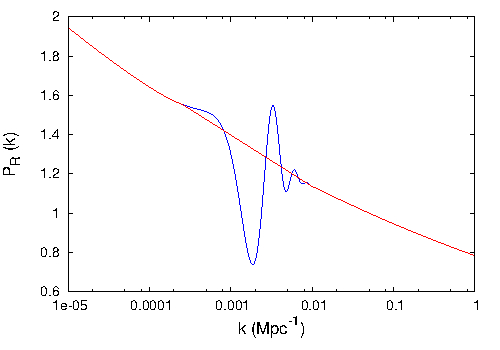
Figure 1: Primordial power spectra for inflationary potentials with step. The red line shows the reference power-law spectrum, while the blue line draws the best-fit spectrum for the inflationary step-like model with $m=7.5$ x $10^{-6}$, using the best-fit values of Benetti:2013cja .

III Analysis method

We performed a set of analyses using four Minkowski Functionals in order to search for non-Gaussian contributions potentially present in simulated and Planck CMB maps. We are primarily interested in answering the following related questions: (i) are there non-Gaussian contributions left in simulated CMB maps generated by the angular power spectra of inflationary step-like models? If the answer is yes, our second question is: (ii) are these non-Gaussian signatures compatible with the last released foreground-cleaned Planck CMB maps?

In fact, if one finds non-Gaussian contributions in simulated maps produced from the CMB power spectra obtained from inflationary step-like models, then we can infer that these NGs are of primordial origin. For this the pertinency of the second question, to discover whether these non-Gaussian features are present, or not, in the foreground-cleaned Planck maps.

III.1 The Models

We start our analysis from the results of the previous work of Benetti Benetti:2013cja , using the following values for the cosmological and step parameters: $100\,\Omega_{b}h^{2}=2.22$, $\Omega_{c}h^{2}=0.1212$, $\tau=0.089$, $100\,\theta=1.0411$, $n_{s}=0.959$, $10^{9}A_{s}=2.20$, $b=14.66$, $c=1.4\times 10^{-3},\,d=3.6\times 10^{-2}$, and we called this model as Model A.

We also consider a second model, called Model B, using the same cosmological and step parameters values of the previous model with the exception of the step amplitude parameter $c$, that is four times higher than in the Model A.

We performed a Monte Carlo Markov Chain analysis via the publicly available package CosmoMC Lewis:2002ah and used a modified version of the CAMB (camb ) code in which we numerically solve Eqs. (1)–(4) using a Bulirsch-Stoer algorithm in order to theoretically calculate the initial perturbation spectrum Eq. (5) needed to compute the CMB anisotropies spectrum. The resulting CMB power spectra for the Model A (dashed line) and Model B (dot-dashed line) are showed in Figs. (2) and (3), together with the featureless $\Lambda$CDM angular power spectrum (continuous line).

III.2 The Minkowski Functionals

The Minkowski Functionals (MF) present many advantages as compared with other statistical estimators, between them one can mention their versatility to detect diverse types of NG without a previous knowledge of their features, like their intensity or angular dependance, and also because they can be efficiently applied in sky patches or masked maps.

All the morphological properties of a $d$-dimensional space can be described using $d+1$ MFs (1903/minkowski, ). In the case of a 2-dimensional CMB temperature field defined on the sphere, $\Delta T=\Delta T(\theta,\phi)$, with zero mean and variance $\sigma^{2}$, this tool provides a test of non-Gaussian features by assessing the properties of connected regions in the map. Given a sky path ${\cal P}$ of the pixelized CMB sphere ${\cal S}^{2}$, an excursion set of amplitude $\nu_{t}$ is defined as the set of pixels in ${\cal P}$ where the temperature field exceeds the threshold $\nu_{t}$, that is, the set of pixels with coordinates $(\theta,\phi)\in{\cal P}$ such that $\Delta T(\theta,\phi)/\sigma\equiv\nu>\nu_{t}$. Each excursion set, or connected region, $\Sigma$, with $\nu>\nu_{t}$, and its boundary, $\partial\Sigma$, can be defined as

$$\Sigma \equiv \{(\theta,\phi)\in\mathcal{P}~{}|~{}\Delta T(\theta,\phi)>\nu\sigma_{0}\},$$ (8)

$$\partial\Sigma \equiv \{(\theta,\phi)\in\mathcal{P}~{}|~{}\Delta T(\theta,\phi)=\nu\sigma_{0}\}.$$ (9)

In a two-dimensional case, for a region $\Sigma\subset{\cal S}^{2}$ with amplitude $\nu_{t}$ the partial MFs calculated just in $R_{i}$ are: $a_{i}$, the Area of the region described by $\Sigma$, $l_{i}$, the Perimeter, or contour length, $\partial\Sigma$ of this region, and $n_{i}$, the number of holes inside $\Sigma$. The global MFs are obtained calculating these quantities for all the connected regions with height $\nu>\nu_{t}$. Then, the total Area $A(\nu)$, Perimeter $L(\nu)$ and Genus $G(\nu)$ are (1999/novikov, ; 2006/naselsky_book, ; 2012/ducout, )

$$\!A(\nu) = \frac{1}{4\pi}\int_{\Sigma}d\Omega=\sum a_{i}\,,$$ (10)

$$\!L(\nu) = \frac{1}{4\pi}\frac{1}{4}\int_{\partial\Sigma}dl=\sum l_{i}\,,$$ (11)

$$\!G(\nu) = \frac{1}{4\pi}\frac{1}{2\pi}\int_{\partial\Sigma}\kappa dl=\sum g_{i}=N_{hot}-N_{cold}\,,$$ (12)

where $d\Omega$ and $dl$ are the elements of solid angle and line, respectively. In the Genus definition, the quantity $\kappa$ is the geodesic curvature (for details see, e.g., 2012/ducout ). This last MF can also be calculated as the difference between the number of regions with $\nu>\nu_{t}$ (number of hot spots, $N_{hot}$) and regions with $\nu<\nu_{t}$ (number of cold spots, $N_{cold}$).

The calculations of the MFs used here were done using the algorithm developed by 2012/ducout and 2012/gay . This code calculates four quantities, namely $V_{0}=A(\nu)$, $V_{1}=L(\nu)$, $V_{2}=G(\nu)$, and $V_{3}=N_{clusters}(\nu)$ which are the three usual MFs defined above plus an additional quantity called number of clusters, $N_{clusters}(\nu)$. The latter quantity is the number of connected regions with height $\nu$ greater (or lower) than the threshold $\nu_{t}$ if it is positive (or negative), i.e., the number of hot (or cold) spots of the map.

III.3 Data description

The five sets of simulated maps we investigate here were produced with ${\rm\,N}_{\mbox{\small side}}=512$, and in the case of the Planck CMB maps, they were degraded to this resolution, using the HEALPix (Hierarchical Equal Area iso-Latitude Pixelization) pixelization grid (2005/gorski, ). In this section we give more details about these sets of synthetic maps as well as the Planck maps in analysis.

III.3.1 The Monte Carlo CMB maps

For our analyses we produce five sets of Monte Carlo (MC) CMB maps, random realisations considering a given CMB angular power spectrum. Each set is composed by $1000$ CMB maps. The first three MC sets are seeded by: (i) the $\Lambda$CDM angular power spectrum, according to last Planck results (solid line in Fig. 2); (ii) Model A, corresponding to the best-fit of Planck angular power spectrum data using an inflationary model with step-like potential (dashed line in Fig. 2); (iii) Model B, which also uses an inflationary model with step-like potential but fits less accurately the Planck data (dot-dashed line in Fig. 2).

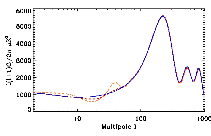
Figure 2: Angular power spectra seeding the spectra of the sets of simulated CMB maps analysed here: the $\Lambda$CDM (solid blue line), the Model A (dashed red line; see text for details), and the Model B (dot-dashed orange line; see text for details).

The last two sets of MC CMB maps are also generated using the $\Lambda$CDM power spectrum, but including different contributions of local-NG, namely, (iv) with $f_{\rm\,NL}=38$, and (v) with $f_{\rm\,NL}=100$, the last set. The first one is chosen to be consistent with recent constraints found by Planck 2013/planck-XXIV ; 2015/planck-XVII , that is, $f_{\rm\,NL}=38\pm 18$ (at 68% confidence level) for the large angular scales. Moreover, our choice for $f_{\rm\,NL}=100$ aims to test also a local non-Gaussian contribution with higher amplitude in order to compare the signatures they produce in the MFs. These latter two sets of non-Gaussian CMB maps were generated from a set of coefficients $a_{\ell\,m}$ derived from a combination of the multipole expansion coefficients $\{a^{\mbox{\footnotesize G}}_{\ell\,m}\}$ and $\{a^{\mbox{\footnotesize NG}}_{\ell\,m}\}$ corresponding to CMB Gaussian and non-Gaussian (of local type) maps, respectively. A set of each kind of these spherical harmonics coefficients, 1000 linear and 1000 non-linear, were produced by 2009/elsner , and are publicly available. We combine these data as follows

$$\,a_{\ell\,m}=a^{\mbox{\footnotesize G}}_{\ell\,m}+f_{\rm\,NL}\,a^{\mbox{\footnotesize NG}}_{\ell\,m}\,,$$ (13)

which were then normalised by the Planck best fit power spectra (2014/planck-XV, ), rescaling $a^{\mbox{\footnotesize G}}_{\ell\,m}$ by the ratio of the square root of the power spectra and $a^{\mbox{\footnotesize NG}}_{\ell\,m}$ directly by the ratio of the power spectra. This linear combination permits to derive CMB synthetic maps with an arbitrary level of of local-NG defined by any real value of $f_{\rm\,NL}$.

As can be observed in Fig. 2, the main differences between the $\Lambda$CDM power spectrum and those from Models A and B are mainly concentrated at large scales, specifically for $\ell=10-50$. For this reason all our analysis will be done focusing on this range of the angular power spectra. That is, in all the MC CMB maps here analysed we consider only the angular scales of this range of multipoles, i.e., $\ell=10-50$ (see Fig. 3).

III.3.2 The foreground-reduced Planck CMB data

In February 2015, the Planck Collaboration released the second set of products derived from the full Planck dataset . Between them are the four CMB foreground-cleaned maps, namely Spectral Matching Independent Component Analysis ($\mathtt{SMICA}$), Needlet Internal Linear Combination ($\mathtt{NILC}$), Spectral Estimation Via Expectation Maximization ($\mathtt{SEVEM}$), and the Bayesian parametric method $\mathtt{Commander}$, names originated from the separation method used to produce them (2015/planck-IX, ). The performance of the foreground-cleaning algorithms has been carefully investigated by the Planck collaboration with various sets of simulated maps. These high resolution maps have ${\rm\,N}_{\mbox{\small side}}=2048$ and effective beam ${\rm FWHM}=5$ arcmin.

In particular, each component separation algorithm processed differently the multi-contaminated sky regions obtaining, as a consequence, different final foreground-cleaned regions for each procedure. These regions are defined outside the so-called Component Separation Confidence masks (briefly termed CS-masks), which have $f_{sky}=0.85,0.96,0.84,0.82,$ for the $\mathtt{SMICA}$, $\mathtt{NILC}$, $\mathtt{SEVEM}$, and $\mathtt{Commander}$ maps, respectively. Each CMB map was released with its own CS-mask, outside which the corresponding CMB signal is considered statistically robust. Regarding the masks, it is worth mentioning that the Planck team produced the $\mathtt{UT78}$ mask, which is the union of the above mentioned masks, a more restrictive one, since it has $f_{sky}\simeq 0.78$, and adopted as the preferred mask for analysing the temperature maps (2015/planck-IX, ).

All the analyses here are performed upon the products of the Planck’s second data release. Moreover, we analyse both the simulated and the four foreground-cleaned Planck CMB maps using two masks, namely, $\mathtt{UT78}$ and the $\mathtt{Commander}$ CS-mask (hereafter, $\mathtt{Commander}$-mask). Since the interesting region of the angular power spectrum for the current analysis corresponds to $\ell=10-50$ (see Fig. 3), we performed some preliminary steps upon each Planck CMB map before proceeding. These steps are: (1) to degrade the maps to ${\rm\,N}_{\mbox{\small side}}=512$, (2) to calculate the angular power spectrum of each one, and (3) to generate the CMB maps from the selected range of multipoles. These final maps are the ones we analyse in the next section.

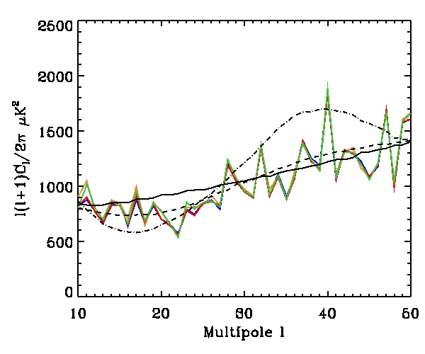
Figure 3: The multipoles range of the seeded angular power spectra for the MC CMB maps, namely, $\Lambda$CDM (solid line), Model A (dashed line), and Model B (dot-dashed line). The blue, orange, red, and green curves correspond to the spectra calculated from the $\mathtt{SMICA}$, $\mathtt{SEVEM}$, $\mathtt{NILC}$ and $\mathtt{Commander}$ maps, respectively.

IV Results and Discussion

Considering $n$ different thresholds $\nu=\nu_{{}_{1}},\nu_{{}_{2}},...\,\nu_{n}$, previously defined dividing the range $-\nu_{max}$ to $\nu_{max}$ in $n$ equal parts, we compute the four MFs $\{V_{k},\,k=0,1,2,3\}\equiv(V_{0},V_{1},V_{2},V_{3})$ for the $i$-th simulated map, with $i=1,2,...,1000$. Then, for the $i$-th map and for $k$-th MF we have the vector

$$\,\,\mathrm{v}_{k}^{i}\equiv(V_{k}(\nu_{{}_{1}}),V_{k}(\nu_{{}_{2}}),...V_{k}(\nu_{n}))|_{\mbox{\small for the $i$-th map}}\,.$$ (14)

In this work the values chosen for such variables are $\{\nu_{max},n\}=\{3.5,26\}$ (for details, see (2012/ducout, )).

IV.1 Performance of the MFs as non-Gaussian estimators

Firstly we investigate the performance of the four MFs by quantifying how large (in relative difference) is the deviation signal in the presence of local-NG in simulated maps, as compared with the results obtained in the analysis of the set of Gaussian $\Lambda$CDM CMB maps. For this reason we consider sets of simulated CMB maps with the same type of local-NG, but different amounts of such contribution, namely with $f_{\rm\,NL}=38$ and $f_{\rm\,NL}=100$, sets (iv) and (v), respectively. A similar situation happens for the MC sets (ii) and (iii), corresponding to Models A and B, respectively.

We show in Fig. 4 our analyses of the four MFs, including a comparison using two masks: the $\mathtt{UT78}$ mask (left column) and the $\mathtt{Commander}$-mask (right column). From top to bottom we analyse the MFs: Area, Perimeter, Genus, and N_clusters, respectively. In all the panels we show the mean value of the corresponding MF obtained for each of the five sets of 1000 MC maps (we illustrate these curves using different colours). We also plot the shadow region corresponding to $1\sigma$ values of the Gaussian $\Lambda$CDM, i.e., MC set (i). At first sight, Area and Genus seems not sensible to the different non-Gaussian contents in the sets of MC CMB maps. From other side, for the Perimeter and N_clusters MFs, and for the Genus case when the $\mathtt{Commander}$-mask is used, some curves appear close and indistinguishable. For this we find interesting to plot the relative difference between the mean curves of the MC sets (ii) to (v) minus the mean curves obtained from the Gaussian $\Lambda$CDM maps, as illustrated in Fig. 5.

In Fig. 5 the left column refers to analyses with the $\mathtt{UT78}$ mask, while the right column refers to analyses with the $\mathtt{Commander}$-mask, just to compare the effect left by the use of different masks. The four rows of such figure, from top to bottom, refers to the four MFs: Area, Perimeter, Genus, and N_clusters, respectively. In each plot the four coloured curves correspond to the relative difference between the mean curves, plotted in Fig. 4, of the corresponding MFs from simulated CMB sets (ii), (iii), (iv), and (v) minus the Gaussian $\Lambda$CDM MC set (i): violet [set (v) - set (i)], green [set (iv) - set (i)], orange [set (iii) - set (i)], and red [set (ii) - set (i)], respectively. It is worth to notice that the vertical scale is not the same for all plots. In the case of the Area-MF, the vertical scale is two orders of magnitude less than the other MFs.

The analyses of these results lead to three important conclusions. First, a single statistical estimator is not sensible enough to detect any non-Gaussian contribution (or a combination of them) present in CMB maps; that is to say: various estimators are more efficient to perform this task. Second, analyses with different cut-sky masks reveal basically the same information, except for the Genus-MF as noticed in the plots of the third row of Fig. 4. Third, and more interestingly, the Gaussian deviations shown in the plots of Fig. 5 makes clear that the set of MFs are able to discriminate distinct NGs imprinted in CMB maps: the non-Gaussian signatures appearing in the sets of MC CMB maps emerging from Models A and B are not of the type, neither intensity, expected in maps contaminated with primordial local-NG, deserving a closer analyses (to be done in the next subsection).

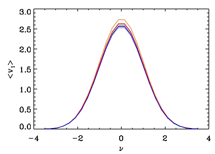
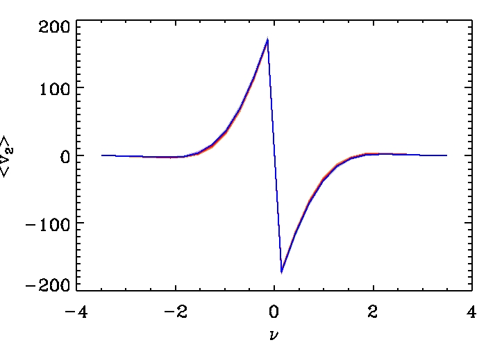
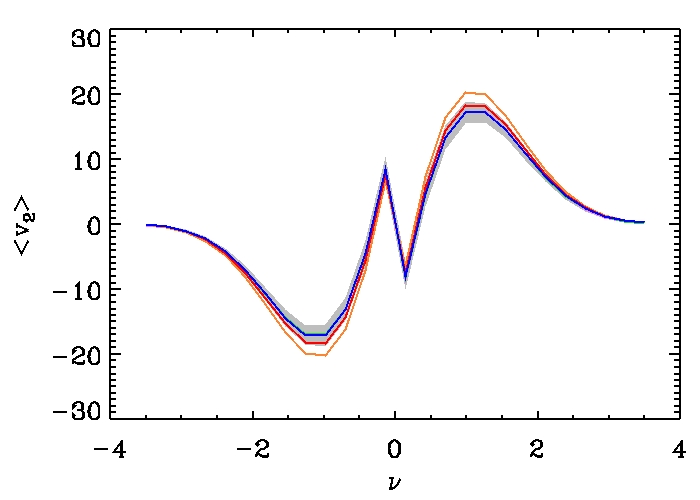
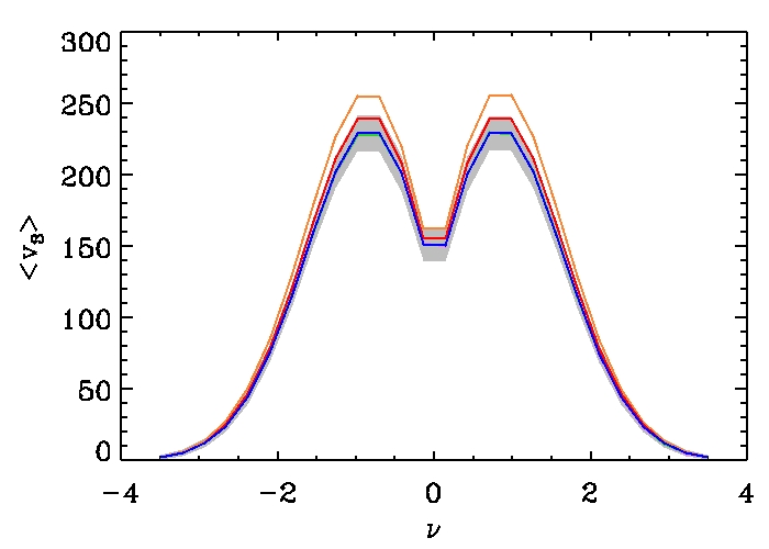
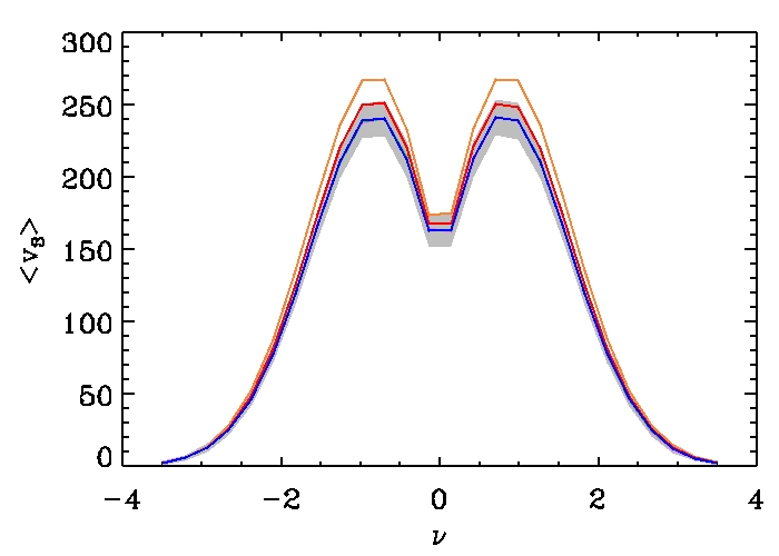
Figure 4: Comparison between the average Area ($\mathrm{v}_{0}$), Perimeter ($\mathrm{v}_{1}$), Genus ($\mathrm{v}_{2}$) and, $N_{clusters}$ ($\mathrm{v}_{3}$) MF vectors over 1000 realisations of each dataset, using the two masks, $\mathtt{UT78}$ (left) and $\mathtt{Commander}$-mask (right). The blue, red, and orange curves corresponds to the average MF obtained from dataset seeded by the $\Lambda$CDM, Model A and Model B power spectra, respectively. The green and violet curves represent the average MFs calculated from MC CMB maps seeded by $\Lambda$CDM power spectra and contaminated by local-NG with $f_{\rm\,NL}=$ 38 and 100, respectively. The gray region represents the 1$\sigma$ level calculated from the MFs curves obtained from the $\Lambda$CDM seeded dataset.

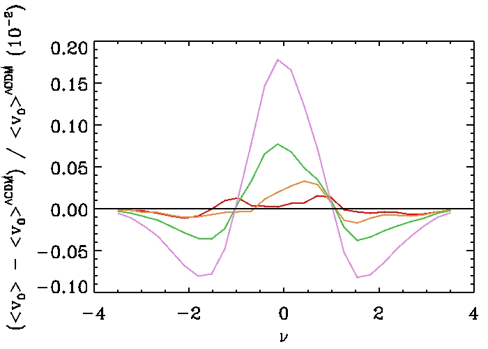
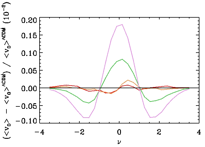
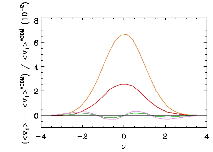
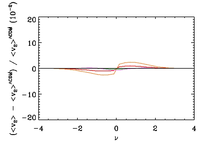
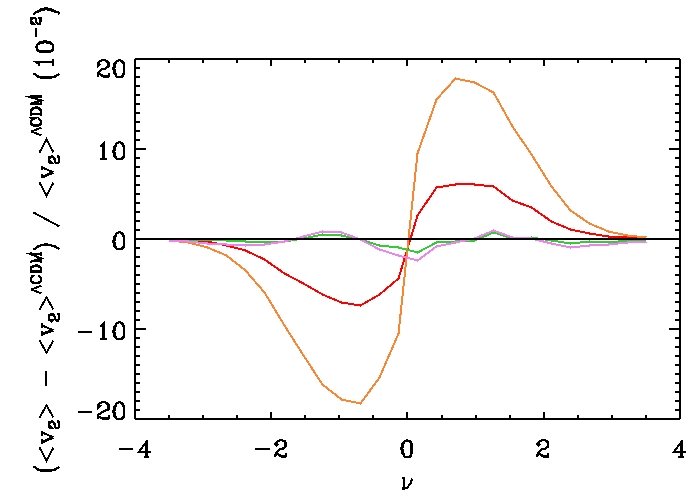
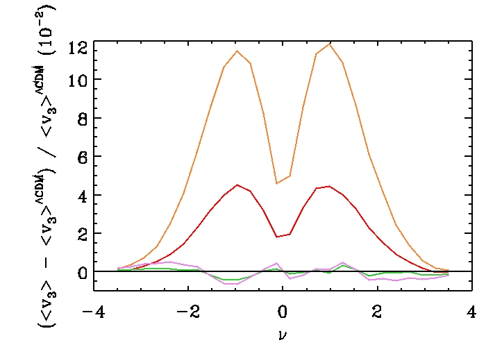
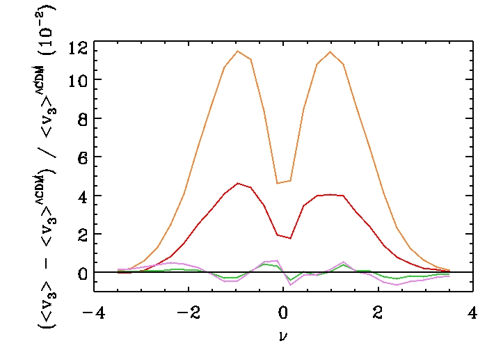
Figure 5: Relative difference between the mean curves plotted in Fig. 4 of the corresponding MFs for the sets of CMB maps (ii) to (v) minus the mean curves obtained for the Gaussian $\Lambda$CDM set (i) (see the text for details about these five sets of MC CMB maps). The left (right) column refers to analyses with the $\mathtt{UT78}$ mask ($\mathtt{Commander}$-mask), to compare the effect left by the use of different masks. From top to bottom the four rows of panels refers to the four MFs: Area, Perimeter, Genus, and N_clusters, respectively. In each plot the four coloured curves correspond to the difference between the MFs from simulated CMB sets (ii), (iii), (iv), and (v) minus the $\Lambda$CDM set, i.e., the Gaussian MC set (i): violet [set (v) - set (i)], green [set (iv) - set (i)], orange [set (iii) - set (i)], and red [set (ii) -set (i)], respectively. It is worth to notice that the vertical scale is not the same for all plots. In the case of the Area-MF, the vertical scale is two orders of magnitude less than the other MFs.

IV.2 Non-Gaussian features in MC CMB maps from Models A and B

Our analyses here are aimed to answer the question: are there distinguishable non-Gaussian features left in simulated CMB maps generated by Models A and B’s angular power spectra? For this, we examine the peculiar imprints left in the sets of CMB maps produced from the power spectra of Models A and B, features that can be revealed by the MFs in comparison with the Gaussian CMB maps generated using the $\Lambda$CDM power spectrum. Remember that the power spectra of these Models were obtained through the CAMB code assuming a step-like potential in the inflation model (these Models differ one to the other in the parameter values of the step-like inflationary potential). It is also worth to notice that Model A fits the CMB angular power spectrum from Planck data better than the $\Lambda$CDM model does (see Fig. 3 in Ref. Benetti:2013cja , and analysis therein); from other side, the angular spectrum from Model B fits the Planck data worse than the $\Lambda$CDM model does.

Our analyses of the four CMB data sets, that is, the MC sets (ii) to (v), show consistency at a 1$\sigma$ level with the MFs obtained from the Gaussian $\Lambda$CDM maps, as seen in Fig. 4. For this, to go further in the current scrutiny we explore the relative difference curves between the mean MF from a given MC set, from set (ii) to set (v), and the corresponding mean MF obtained for the set (i), that is the set of Gaussian $\Lambda$CDM CMB maps. Our examinations show, except in the Area-MF case, that the CMB maps seeded by the power spectra of Models A (set (ii)) and B (set (iii)) evidence a larger Gaussian deviation, with fully distinct signature, as compared with the results from the MC CMB maps contaminated with primordial local-NG, with $f_{\rm\,NL}=38$ (set (iv)) and $f_{\rm\,NL}=100$ (set (v)).

In fact, one verifies in the panels of the second, third, and fourth rows of Fig. 5, that a distinguished departure from Gaussianity comes from the analyses of these CMB data produced from Models A and B, with the remarkable feature that for the Model B case the Gaussian deviation appears with the same signature than for the Model A case but it is notoriously larger. In other words, inflationary Models A and B produce a noticeable (in type and intensity) Gaussian deviation as measured by the MFs, where they are best revealed by the Perimeter and N_clusters MFs, and less efficiently by the Genus, beside being robust under different masks applied.

All these results let us to conclude that the non-Gaussian signals found in the MC maps seeded by the CMB power spectra from inflation Models A and B are contributions with a definite signature originated in the inflationary phase, suggesting an effective probe to the primordial universe.

IV.3 Mapping non-Gaussian signatures in Planck maps

The third part of our analyses concerns the calculation of the MFs from the four foreground-cleaned Planck CMB maps, considering the above mentioned masks. In Figs. 6 to 9 we present the relative difference between the MFs calculated for each one of these Planck maps and the corresponding MF mean obtained for the five sets of MC CMB maps. In Tables 1 (for the $\mathtt{UT78}$ mask) and 2 (for the $\mathtt{Commander}$-mask) we show the $\chi^{2}$ values, for 25 degrees of freedom, corresponding to the best-fit between the MF from the Planck map and the mean MF for each of the five MC sets in scrutiny. First of all, our results confirm the point raised above regarding the performance between the four MFs. As a matter of fact, the Area (Fig. 6) and Genus (Fig. 8) functionals appear to be the less conclusive, each one presenting quite similar differences for all the four Planck maps and for both masks. Regarding the Perimeter (Fig. 7) and N_clusters (Fig. 9), the panels show a great concordance between Gaussian and non-Gaussian (i.e., $f_{\rm\,NL}\neq 0$) $\Lambda$CDM seeded maps, presenting just tiny relative differences for the four Planck maps. In these figures we also observe that comparing the cases regarding Models A and B, they exhibit the same signature but very different intensity, being clear that the Perimeter and N_clusters functionals from the Model A fits better the four Planck maps. Additionally, this last result is corroborated by the $\chi^{2}$ analyses, being valid for both masks (see Tables 1 and 2). In other words, our MF’s analyses reveal that the non-Gaussian signatures observed in the four foreground-cleaned Planck maps are better represented by those appearing in the set of MC CMB maps generated from the Model A angular power spectrum (i.e., the MC set (ii)).

Table 1: $\chi^{2}$ values calculated from the MFs (Area ($\mathrm{v}_{0}$), Perimeter ($\mathrm{v}_{1}$), Genus ($\mathrm{v}_{2}$), and $N_{clusters}$ ($\mathrm{v}_{3}$)) curves obtained for each Planck map and the average MFs over 1000 realisations of the sets: (i) to (v). All the MFs considered here are calculated using the cut-sky corresponding to the $\mathtt{UT78}$ mask. The number of degrees of freedom is 25.

MF	Planck	Data seta
	map	(i)	(ii)	(iii)	(iv)	(v)
$\mathrm{v}_{0}$	$\mathtt{SMICA}$	34.0	35.9	39.8	36.7	42.1
	$\mathtt{NILC}$	34.3	36.3	40.3	37.3	43.0
	$\mathtt{SEVEM}$	33.8	35.6	39.6	36.0	41.0
	$\mathtt{\,\,Commander\,\,}$	33.0	34.9	38.8	35.5	40.9
$\mathrm{v}_{1}$	$\mathtt{SMICA}$	26.2	21.0	78.4	29.5	34.1
	$\mathtt{NILC}$	27.1	22.9	82.3	30.5	35.3
	$\mathtt{SEVEM}$	24.8	24.9	92.3	27.7	32.2
	$\mathtt{\,\,Commander\,\,}$	27.2	23.4	83.5	30.5	35.1
$\mathrm{v}_{2}$	$\mathtt{SMICA}$	44.6	43.8	47.3	48.4	51.3
	$\mathtt{NILC}$	47.7	47.8	50.3	54.5	58.2
	$\mathtt{SEVEM}$	40.4	39.2	43.0	43.5	45.8
	$\mathtt{\,\,Commander\,\,}$	44.7	43.5	46.7	48.0	50.4
$\mathrm{v}_{3}$	$\mathtt{SMICA}$	22.0	23.5	57.9	23.7	26.3
	$\mathtt{NILC}$	27.1	26.1	55.3	29.8	32.5
	$\mathtt{SEVEM}$	18.6	18.4	50.3	18.7	20.1
	$\mathtt{\,\,Commander\,\,}$	30.0	30.9	63.9	30.1	31.7
aThe data sets correspond to: MC CMB maps seeded by (i) $\Lambda$CDM, (ii) Model A, and (iii) Model B angular power spectra, and two other $\Lambda$CDM seeded sets, but including contributions of local-NG, namely, (iv) $f_{\rm\,NL}=38$, and (v) $f_{\rm\,NL}=100$.

Table 2: $\chi^{2}$ values. Same as in Table 1, but for MFs calculated using the cut-sky corresponding to the $\mathtt{Commander}$-mask. The number of degrees of freedom is 25.

MF	Planck	Data set
	map	(i)	(ii)	(iii)	(iv)	(v)
$\mathrm{v}_{0}$	$\mathtt{SMICA}$	31.9	33.5	37.5	34.0	38.9
	$\mathtt{NILC}$	32.6	34.3	38.4	35.1	40.3
	$\mathtt{SEVEM}$	31.5	33.1	37.1	33.0	37.3
	$\mathtt{\,\,Commander\,\,}$	31.1	32.6	36.6	32.8	37.3
$\mathrm{v}_{1}$	$\mathtt{SMICA}$	28.8	19.4	77.3	30.4	34.6
	$\mathtt{NILC}$	29.7	21.5	82.0	31.3	35.8
	$\mathtt{SEVEM}$	27.7	22.9	89.4	28.8	32.7
	$\mathtt{\,\,Commander\,\,}$	29.9	22.4	83.8	31.4	35.5
$\mathrm{v}_{2}$	$\mathtt{SMICA}$	20.5	10.1	18.5	20.9	22.5
	$\mathtt{NILC}$	35.2	23.8	28.1	37.4	40.2
	$\mathtt{SEVEM}$	25.6	13.6	19.8	25.2	26.3
	$\mathtt{\,\,Commander\,\,}$	28.4	17.3	23.5	28.6	30.2
$\mathrm{v}_{3}$	$\mathtt{SMICA}$	13.2	13.5	48.2	13.8	15.7
	$\mathtt{NILC}$	27.3	23.0	49.9	28.6	31.5
	$\mathtt{SEVEM}$	13.8	12.8	45.6	14.0	15.7
	$\mathtt{\,\,Commander\,\,}$	18.3	19.6	55.2	18.4	20.2

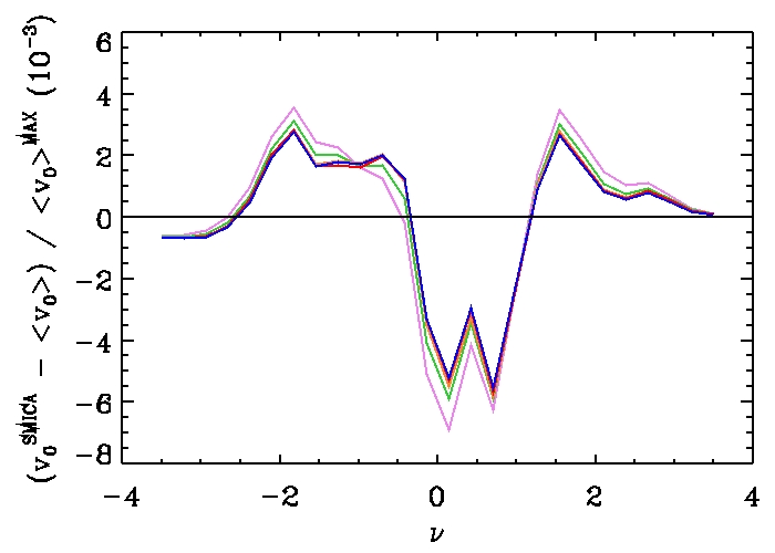
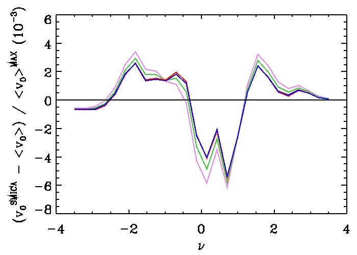
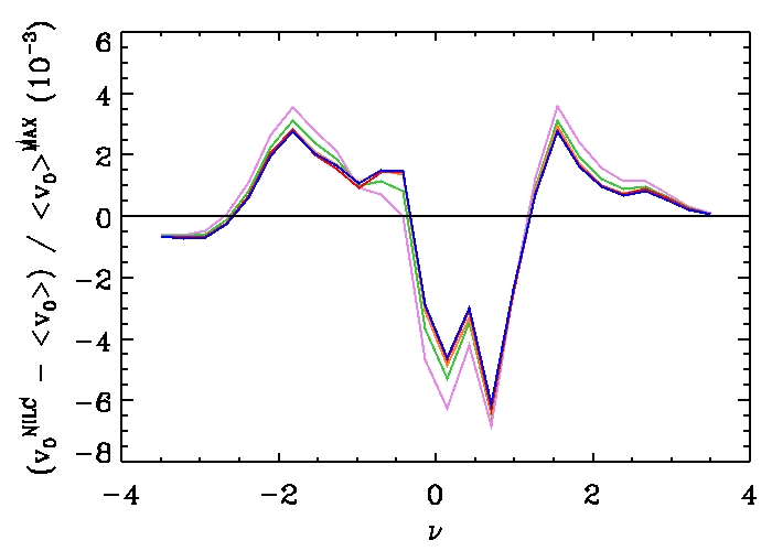
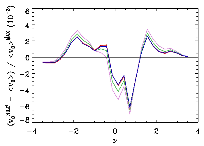
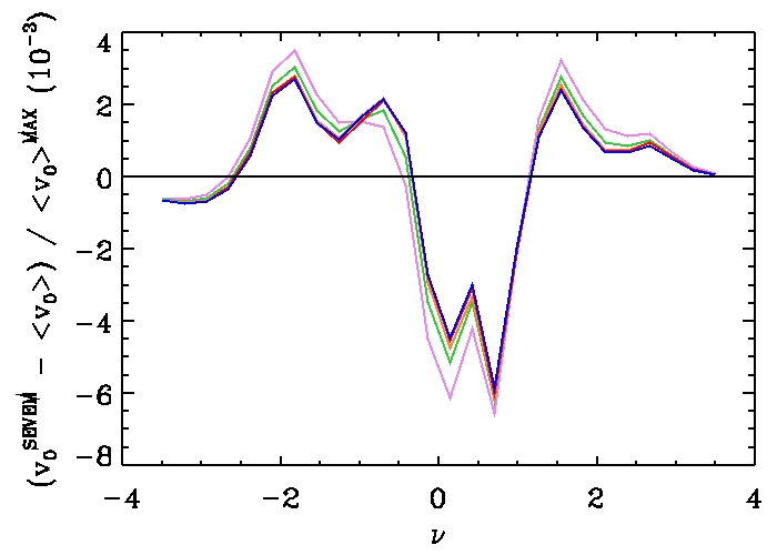
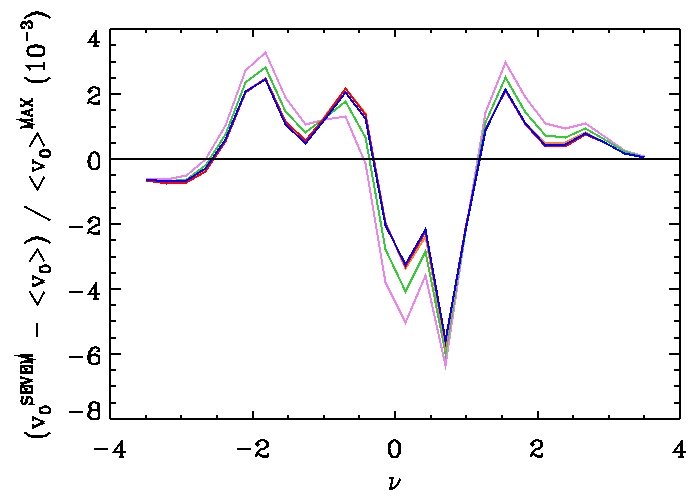
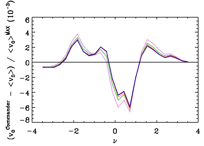
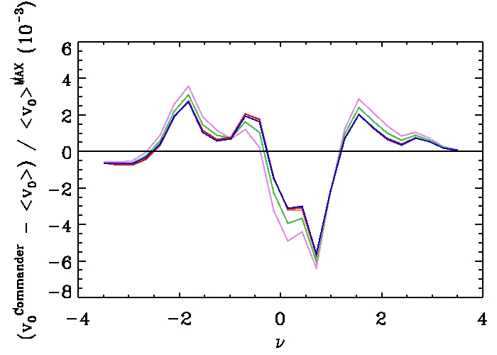
Figure 6: Relative difference between the Area-MF vectors ($\mathrm{v}_{0}$) calculated from each Planck map (from top to bottom: $\mathtt{SMICA}$, $\mathtt{NILC}$, $\mathtt{SEVEM}$ and $\mathtt{Commander}$ maps, respectively) and the average Area-MF ($\langle\mathrm{v}_{0}\rangle$) obtained from the five sets of MC CMB maps, namely, $\Lambda$CDM seeded Gaussian (blue) and non-Gaussian ($f_{\rm\,NL}=$ 38 and 100; green and violet, respectively) maps, and Model A (red) and Model B (orange) seeded maps. The left and right panels correspond, respectively, to the analyses performed using the masks $\mathtt{UT78}$ and $\mathtt{Commander}$-mask.

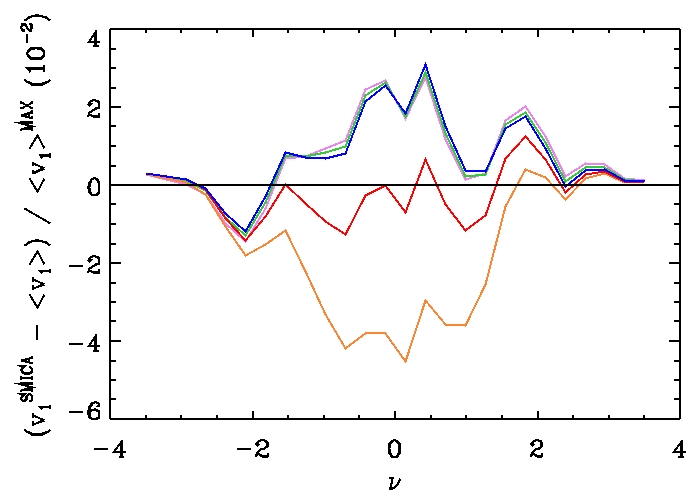
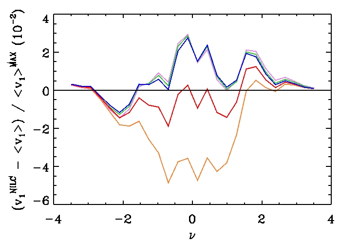
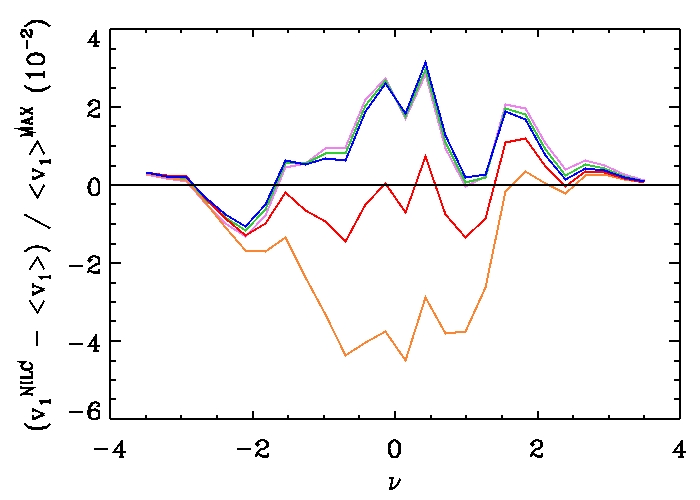
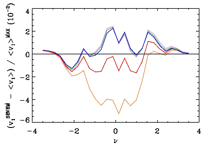
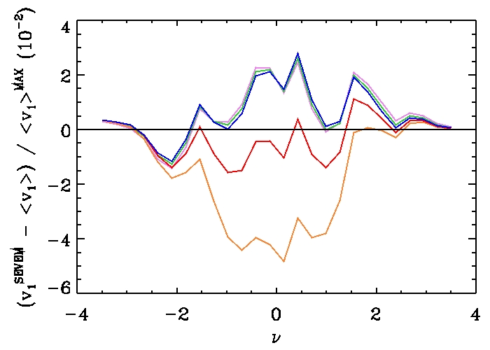
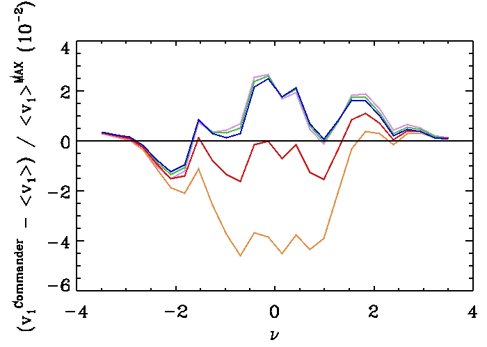
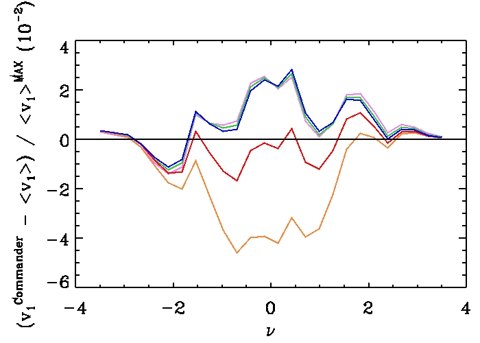
Figure 7: Same as in Fig. 6, but for the Perimeter-MF vectors.

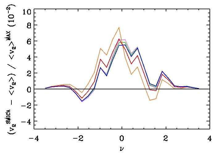
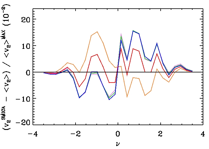
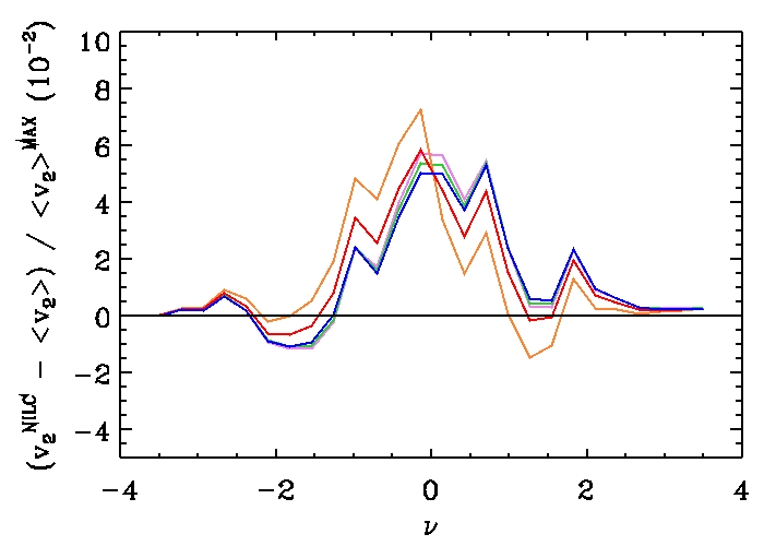
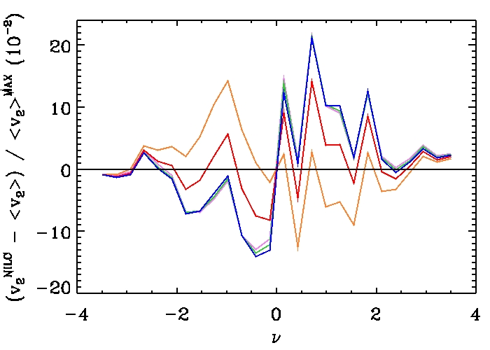
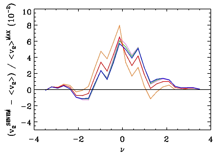
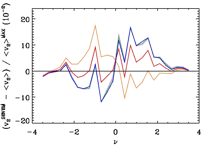
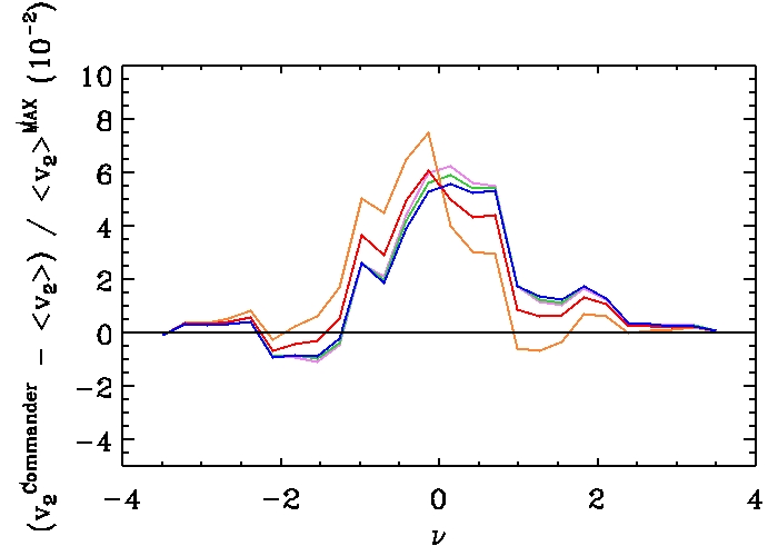
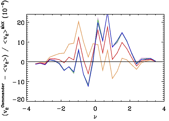
Figure 8: Same as in Fig. 6, but for the Genus-MF vectors.

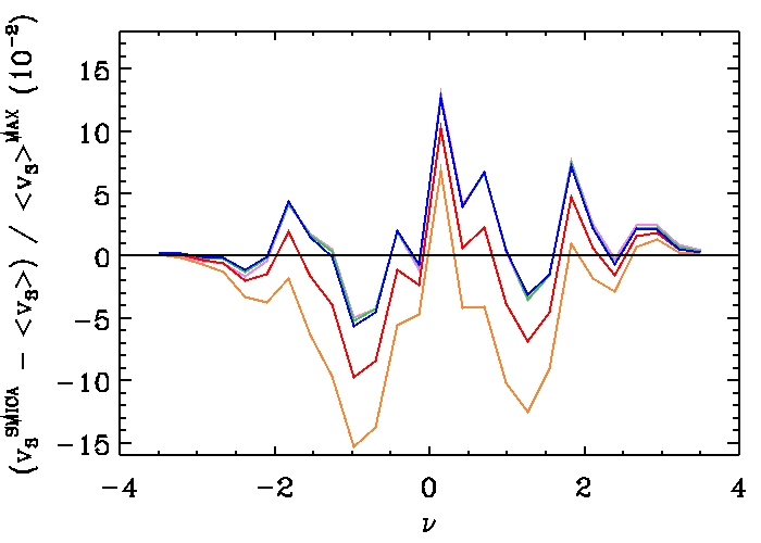
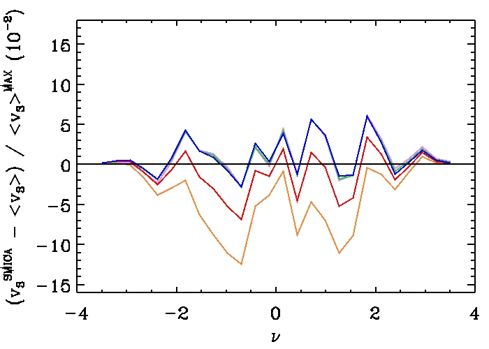
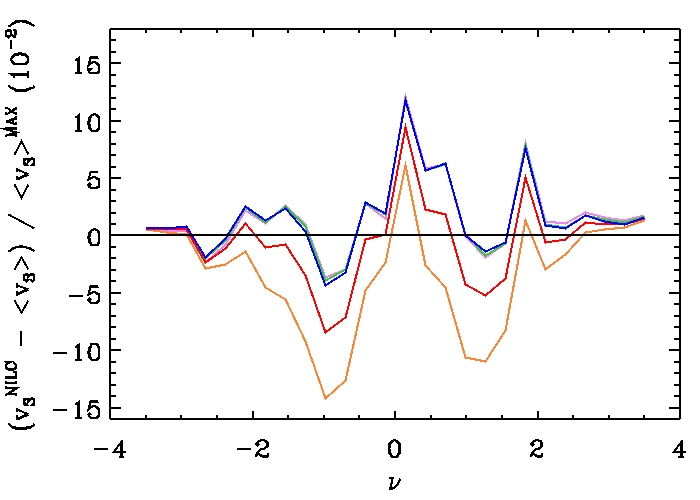
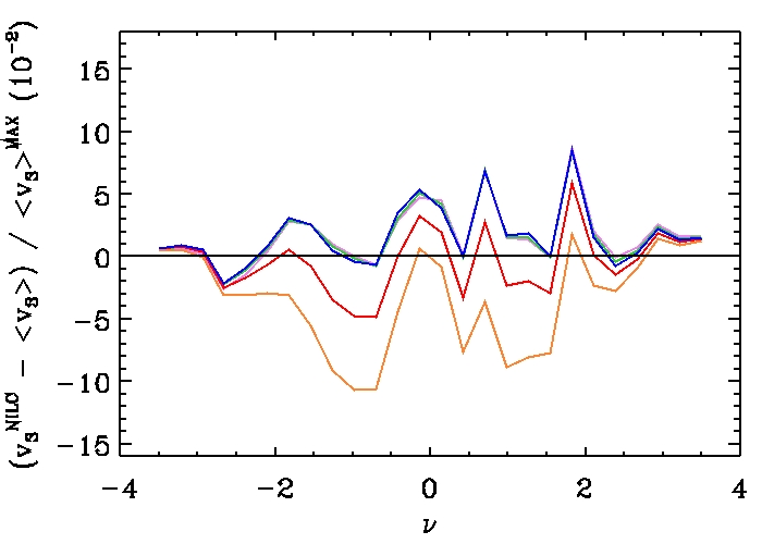
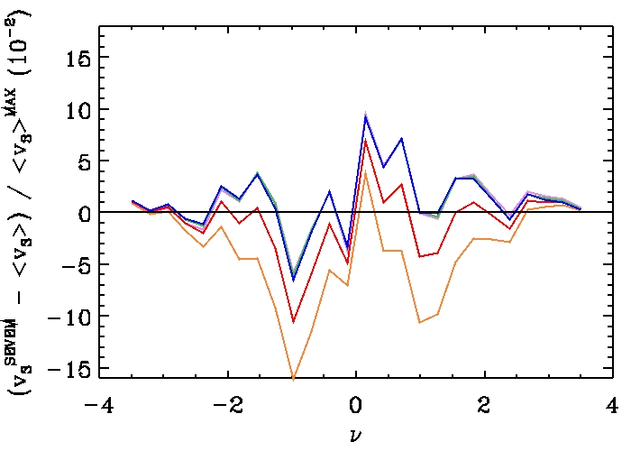
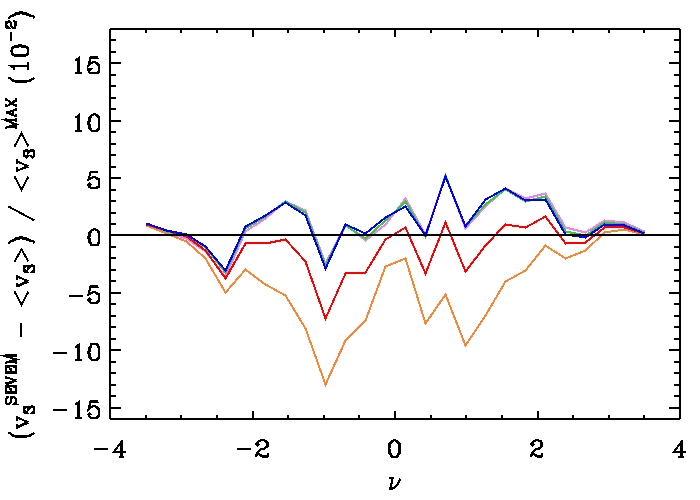
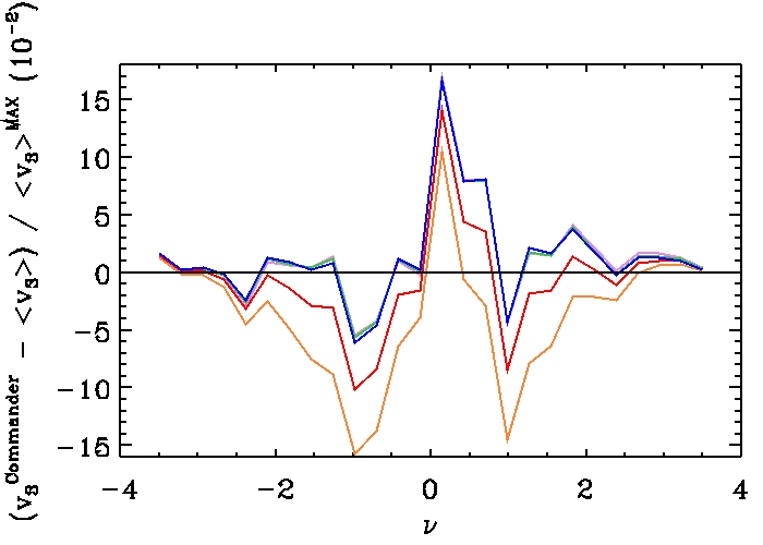
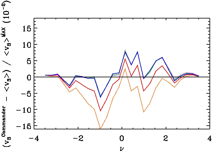
Figure 9: Same as in Fig. 6, but for the $N_{clusters}$-MF vectors.

V Concluding Remarks

The main purpose of this work is the analyses of non-Gaussian signatures originated in the inflation models with a step-like feature in the primordial potential. Such models produce oscillatory features in the primordial spectrum of scalar perturbations, whose effect on the CMB temperature fluctuations can be tested through the analyses of simulated CMB maps seeded by the power spectrum generated by this model. Here we employed four MFs to search for possible Gaussian deviations in such synthetic CMB maps.

Using the five sets of MC CMB maps, and examining the effect of using two different cut-sky masks, our analyses initiate by testing the sensitivity of the four MFs to local-NG, with two different amplitudes, and that NGs probably produced by the inflationary Models A and B. A first conclusion is that, between the four quantities, the Genus-MF is the main affected by the cut-sky. We also found that the MFs are able to discriminate the different types and amplitudes of NGs. This statement is firstly observed from the results presented on Figs. 4 and 5, which display the different features of the local-NG compared to that ones imprinted on CMB by Models A and B. In fact, for the current analyses, we find the following order in sensitivity for the MFs: Perimeter $>$ N_clusters $>$ Genus $\gg$ Area, from the most to the least sensitive, respectively. This result is inferred from the amplitude of the corresponding relative differences observed in Fig. 5, as well as from the $\chi^{2}$ values shown in Tables 1 and 2.

The detection of Gaussian deviations, as evidenced by departures of the MFs curves compared with the corresponding ones from Gaussian CMB maps, clearly suggest the presence of non-Gaussian signals. Exploring this inference more carefully, we analysed the relative difference between the mean MFs obtained from the four sets of maps, sets (ii) to (v), and that one corresponding to Gaussian simulations, set (i), seeded by the $\Lambda$CDM power spectrum. From the obtained results, it is inferred that MC CMB maps generated from Models A and B power spectra present a clear Gaussian deviation, better described by the perimeter-MF analyses as shown in Fig. 7 and quantified by the $\chi^{2}$ values in Tables 1 and 2 , whose source is not other than the known ‘features’ that characterise these models (see Figs. 2 and 3), therefore originated in the primordial inflationary phase. Moreover, it was possible to reveal the distinctive signature and amplitude of the Gaussian deviations present in the MC CMB maps seeded by the power spectra from Model A, that one that fits Planck data better than $\Lambda$CDM model, and Model B, when compared to the non-Gaussian simulations (i.e., $f_{\rm\,NL}\neq 0$).

Finally, in the last part of this work we analysed the four foreground-cleaned Planck CMB maps in the current context. The analyses of the relative differences between the MFs of each Planck map and the average MFs from the five sets of MC CMB maps confirm a good agreement between the Planck data and data coming from the MC seeded by Model A power spectrum (i.e., the MC set (ii)). In addition, we use the goodness-of-fit test to get an overall measure of this concordance obtaining the $\chi^{2}$ values presented in Tables 1 and 2, which confirm this result. This lead us to our main conclusion concerning Planck data: non-Gaussian signatures present in the four foreground-cleaned Planck maps are better represented by the MCs CMB maps seeded by Model A power spectrum than is done by those MCs seeded by the $\Lambda$CDM (Gaussian and local non-Gaussian simulations) and Model B power spectra.

Considering that any convincing deviation from Gaussianity results from a robust detection by the MFs, which include analyses with different masks. In addition, such departures are larger when the power spectrum features appears exaggerated (this refers to Model B ‘features’ with respect to those of Model A, see Figs. 2 and 3), then the main conclusions of the current analyses regarding the MC CMB maps derived from inflationary models with a step-like potential (i.e., the MC sets (ii) and (iii)) are:

• The non-Gaussian contributions found in these sets of MC CMB maps are of primordial origin.

• These net Gaussian deviations, as robustly detected by the MFs, are not accounted by primordial local-NG, neither in intensity nor in signature.

• The non-Gaussian signatures in Planck CMB data, as revealed by MFs, are better described by MC maps seeded by Model’s A CMB spectrum.

Additionally, it is opportune to inquire about the type and level of the NG detected. According to the results of Chen et al. Chen06 , inflationary models with a step-like potential would produce detectable levels of NG of equilateral type, with expected amplitude $|f_{\rm\,NL}^{\rm\,equil}|\simeq 10$, for the step parameters considered in Model A. Moreover, as showed in Table 1, the $\chi^{2}$ best-fit satisfied by the MCs from Model A indicates that the NG observed in the foreground-cleaned Planck maps is fully compatible with the NG (of equilateral type as predicted by Chen06 ) found by our perimeter-MF analyses in these MC CMB maps (see Fig. 7). These facts, altogether, show the good agreement between the equilateral NG measured by the Planck collaboration, namely, $f_{\rm\,NL}^{\rm\,equil}=-16\pm 70$ 2015/planck-XVII , and the NG predicted by Chen06 for Model A and detected by the perimeter-MF in the four Planck CMB maps.

VI Acknowledgments

We acknowledge L.R. Abramo for useful comments. CPN and MB acknowledge CAPES and FAPERJ (Brazilian Financial Agencies), respectively, for their fellowships; AB acknowledges a CAPES PVE project. We are grateful for the use of the $\{a^{\mbox{\footnotesize G}}_{\ell\,m}\}$ and $\{a^{\mbox{\footnotesize NG}}_{\ell\,m}\}$ simulations (2009/elsner, ). We also acknowledge the use of CAMB (A. Lewis and A. Challinor: http://camb.info/), and for the MF’s code 2012/ducout ; 2012/gay . Some of the results in this paper have been derived using the HEALPix package 2005/gorski .

References

- (1) P. A. R. Ade et al. (Planck Collaboration), arXiv:1502.01589.
- (2) P. A. R. Ade et al. (Planck Collaboration), arXiv:1502.02114.
- (3) H. V. Peiris et al. (WMAP Collaboration), Astrophys. J. Suppl. 148, 213 (2003), astro-ph/0302225.
- (4) L. Covi, J. Hamann, A. Melchiorri, A. Slosar and I. Sorbera, Phys. Rev. D 74, 083509 (2006), astro-ph/0606452.
- (5) J. Hamann, L. Covi, A. Melchiorri and A. Slosar, Phys. Rev. D 76, 023503 (2007), astro-ph/0701380.
- (6) M. J. Mortonson, C. Dvorkin, H. V. Peiris and W. Hu, Phys. Rev. D 79, 103519 (2009), arXiv:0903.4920.
- (7) D. K. Hazra, M. Aich, R. K. Jain, L. Sriramkumar and T. Souradeep, JCAP 1010, 008 (2010), arXiv:1005.2175.
- (8) P. D. Meerburg, R. Wijers and J. P. van der Schaar, arXiv:1109.5264.
- (9) M. Benetti, M. Lattanzi, E. Calabrese and A. Melchiorri, Phys. Rev. D 84, 063509 (2011), arXiv:1107.4992.
- (10) M. Benetti, S. Pandolfi, M. Lattanzi, M. Martinelli and A. Melchiorri, Phys. Rev. D 87, 023519 (2013), arXiv:1210.3562.
- (11) M. Benetti, Phys. Rev. D 88, 087302 (2013), arXiv:1308.6406.
- (12) V. Miranda and W. Hu, Phys. Rev. D 89, 083529 (2014), arXiv:1312.0946.
- (13) J. A. Adams, B. Cresswell and R. Easther, Phys. Rev. D 64, 123514 (2001), astro-ph/0102236.
- (14) P. Hunt and S. Sarkar, Phys. Rev. D 70, 103518 (2004), astro-ph/0408138.
- (15) A. Ashoorioon, C. van de Bruck, P. Millington and S. Vu, Phys. Rev. D 90, 103515 (2014), arXiv:1406.5466.
- (16) R. H. Ribeiro, JCAP 1205, 037 (2012), arXiv:1202.4453.
- (17) P. Adshead, C. Dvorkin, W. Hu and E. A. Lim, Phys. Rev. D 85, 023531 (2012), arXiv:1110.3050.
- (18) J. Martin and L. Sriramkumar, JCAP 1201, 008 (2012), arXiv:1109.5838.
- (19) M. Park and L. Sorbo, Phys. Rev. D 85, 083520 (2012), arXiv:1201.2903.
- (20) P. A. R. Ade et al. (Planck Collaboration), A&A 571, A24 (2014), arXiv:1303.5084.
- (21) P. A. R. Ade et al. (Planck Collaboration), arXiv:1502.01592.
- (22) X. Chen, Advances in Astronomy 2010, 638979 (2010), arXiv:1002.1416.
- (23) X. Chen, R. Easther and E. A. Lim, JCAP 06, 023 (2007), astro-ph/0611645.
- (24) D. Novikov, H. A. Feldman and S. F. Shandarin, Int. J. Mod. Phys. D 8, 291 (1999).
- (25) E. Komatsu, Class. and Quant. Grav. 27, 124010 (2010), arXiv:1003.6097.
- (26) N. Bartolo, S. Matarrese and A. Riotto, Advances in Astronomy 2010, 157079 (2010), arXiv:1001.3957.
- (27) C. P. Novaes, A. Bernui, I. S. Ferreira and C. A. Wuensche, JCAP 01, 018 (2014), arXiv:1312.3293.
- (28) C. P. Novaes, A. Bernui, I. S. Ferreira and C. A. Wuensche, JCAP 2015, 064 (2015), arXiv:1409.3876.
- (29) A. Bernui and M. J. Rebouças, Phys. Rev. D 81, 063533 (2010), arXiv:0912.0269; Phys. Rev. D 85, 023522 (2012), arXiv:1109.6086.
- (30) H. Minkowski, Volumen und Oberfläche, Mathematische Annalen 57, 447 (1903).
- (31) P. A. R. Ade et al. (Planck Collaboration), A&A 571, A15 (2014), arXiv:1303.5075.
- (32) N. Bartolo, E. Komatsu, S. Matarrese and A. Riotto, Phys. Rept. 402, 103 (2004) [astro-ph/0406398].
- (33) D. Baumann, arXiv:0907.5424 [hep-th].
- (34) J. Lesgourgues, Nucl. Phys. B 582, 593 (2000), hep-ph/9911447.
- (35) J. A. Adams, G. G. Ross and S. Sarkar, Nucl. Phys. B 503, 405 (1997), hep-ph/9704286.
- (36) A. Ashoorioon and A. Krause, hep-th/0607001.
- (37) P. Adshead, W. Hu and V. Miranda, Phys. Rev. D 88, no. 2, 023507 (2013), arXiv:1303.7004.
- (38) P. Adshead, W. Hu, C. Dvorkin and H. V. Peiris, Phys. Rev. D 84, 043519 (2011), arXiv:1102.3435.
- (39) N. Bartolo, D. Cannone and S. Matarrese, JCAP 1310, 038 (2013), arXiv:1307.3483.
- (40) D. K. Hazra, L. Sriramkumar and J. Martin, JCAP 05, 026 (2013), arXiv:1201.0926.
- (41) V. Sreenath, D. K. Hazra and L. Sriramkumar, JCAP 02, 029 (2015), arXiv:1410.0252.
- (42) V. Miranda, W. Hu and C. Dvorkin, Phys. Rev. D 91, no. 6, 063514 (2015), arXiv:1411.5956.
- (43) V. Miranda, W. Hu and P. Adshead, Phys. Rev. D 89, no. 10, 101302 (2014), arXiv:1403.5231.
- (44) Y. F. Cai, F. Chen, E. G. M. Ferreira and J. Quintin, arXiv:1412.4298 [hep-th].
- (45) R. K. Jain, P. Chingangbam, J.-O. Gong, L. Sriramkumar and T. Souradeep, JCAP 0901, 009 (2009), arXiv:0809.3915.
- (46) R. K. Jain, P. Chingangbam, L. Sriramkumar and T. Souradeep, Phys. Rev. D 82, 023509 (2010), arXiv:0904.2518.
- (47) A. Lewis and S. Bridle, Phys. Rev. D 66, 103511 (2002), astro-ph/0205436.
- (48) A. Lewis, A. Challinor, and A. Lasenby, Astrophys. J. 538, 473 (2000), astro-ph/9911177.
- (49) P. D. Naselsky, D. I. Novikov and I. D. Novikov, Cambridge Univ. Press, Cambridge, UK (2006).
- (50) A. Ducout, F. Bouchet, S. Colombi, D. Pogosyan and S. Prunet, MNRAS 429, 2104 (2013), arXiv:1209.1223.
- (51) C. Gay, C. Pichon and D. Pogosyan, Phys. Rev. D 85, 023011 (2012), arXiv:1110.0261.
- (52) K. M. Górski, E. Hivon, A. J. Banday, B. D. Wandelt, F. K. Hansen, M. Reinecke and M. Bartelman, ApJ 622, 759 (2005).
- (53) F. Elsner and B. D. Wandelt, ApJS 184, 264 (2009), arXiv:0909.0009.
- (54) P. A. R. Ade et al. (Planck Collaboration), arXiv:1502.05956.