Time-Reversible Ergodic Maps and the 2015 Ian Snook Prize

Abstract

The time reversibility characteristic of Hamiltonian mechanics has long been extended to nonHamiltonian dynamical systems modeling nonequilibrium steady states with feedback-based thermostats and ergostats. Typical solutions are multifractal attractor-repellor phase-space pairs with reversed momenta and unchanged coordinates, $(q,p)\longleftrightarrow(q,-p)$ . Weak control of the temperature, $\propto p^{2}$ and its fluctuation, resulting in ergodicity, has recently been achieved in a three-dimensional time-reversible model of a heat-conducting harmonic oscillator. Two-dimensional cross sections of such nonequilibrium flows can be generated with time-reversible dissipative maps yielding æsthetically interesting attractor-repellor pairs. We challenge the reader to find and explore such time-reversible dissipative maps. This challenge is the 2015 Snook-Prize Problem.

I Time-Reversible Nonequilibrium Flows

The microscopic gist of the macroscopic Second Law is often pictured as a system’s seeking out more phase-space states. So it seems a bit odd that the idealized nonequilibrium steady states generated by molecular dynamics behave in the opposite wayb1 . The $(q,p)$ states from such atomistic simulations soon become constrained to an ever-shrinking strange attractor. The compensating additional heat-reservoir states are never seen explicitly. Instead they are modelled by time-reversible friction coefficients. These coefficients control temperature or energy and induce steady-state behavior in the system under study.

Unlike real life, the underlying Laws of physics are mostly time-reversible, which means it is puzzling that physics gives a good accounting of real-world observations. Time-reversible mechanical models ( molecular dynamics ) provide clear examples of this conundrum. To illustrate the irreversible behavior of such time-reversible models let us consider the simplest case, a one-dimensional harmonic oscillator (with unit mass and force constant ) exposed to a temperature gradientb2 ; b3 , $T=T(q)$ . The oscillator’s motion is subject to a time-dependent friction coefficient $\zeta(p)$ imposing weak control over the oscillator’s kinetic energy $\langle\ K\ \rangle$ and its fluctuation, $\langle\ K^{2}\ \rangle-\langle\ K\ \rangle^{2}\$ . This oscillator modelb2 generates a three-dimensional “flow” satisfying the three ordinary differential equations of motion :

$$\dot{q}=p\ ;\ \dot{p}=-q-\zeta[\ Ap+B(p^{3}/T)\ ]\ ;\ \dot{\zeta}=A[\ (p^{2}/T)-1\ ]+B[\ (p^{4}/T^{2})-3(p^{2}/T)\ ]\ .$$

The superior dots in the motion equations indicate comoving time derivatives.

At thermal equilibrium where $T$ is constant the parameters $(A,B)$ are chosen to promote the control of the second and fourth velocity momentsb3 :

$$(A,B)=(0.05,0.32)\longrightarrow\langle\ (p^{2}/T),(p^{4}/T^{2})\ \rangle=(1,3)\ .$$

From the visual standpoint this parameter choice appears to provide an ergodic coverage of the oscillator phase space. Liouville’s continuity equation in phase space can be used to show that these motion equations are consistent with Gibbs’ canonical distribution ;

$$f(q,p,\zeta)_{\epsilon=0}\propto e^{-q^{2}/2T}e^{-p^{2}/2T}e^{-\zeta^{2}/2}\ .$$

Away from equilibrium the heat-reservoir temperature field $T=1+\epsilon\tanh(q)$ is an explicit function of the oscillator coordinate $q$ and $\epsilon$ is the maximum value of the temperature gradient.

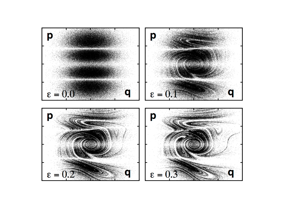
Figure 1: These cross sections can be viewed as generated by time-reversible “dynamical maps”, advancing the dynamics from one penetration of the $\zeta=0$ plane to the next. These $(q,p)$ phase-space cross sections for the conducting oscillator correspond to four values of the maximum temperature gradient : $\epsilon=0.0,\ 0.1,\ 0.2,\ {\rm and}\ 0.3$ . Both $q$ and $p$ range from $-4$ to $+4$ in all the cross sections.

See Figure 1 for sample numerical $(q,p)$ cross sections of the three-dimensional flow in $(q,p,\zeta)$ space. The $(q,p)$ points are plotted whenever $\zeta$ changes sign. Notice that the equations of motion for this heat-conduction model are time-reversible. To see this start out with a solution of the equations forward in time, $q(t),p(t),\zeta(t)$ . Then change the signs of the momentum $p$, $\zeta$, as well as the direction of time, $(\ +d/dt\rightarrow-d/dt\ )$ . These steps provide a new “reversed” solution of exactly the same motion equations.

The nonequilibrium $(q,p)$ cross-sections with $\epsilon>0$ shown in Figure 1 look like inhomogenous ( or “ multifractal” ) strange attractors. And they are. In these flows, as in a wide variety of time-reversible nonequilibrium steady states, the fractal strange attractors satisfy the Second Law of Thermodynamics, with an overall hot-to-cold heat current. The reversed flows, topologically similar fractals, are mechanically unstable, with exponentially growing phase volume, and with a heat-flow direction violating the second law. These repellor states are unobservable numerically due to this ( Lyapunov ) instability, and can only be collected by storing, and then reversing, a time series of attractor statesb1 .

II Equivalent Time-Reversible Mapsb4 ; b5

The construction of the flow cross-sections is equivalent to applying a time-reversible “map” ${\cal M}(q,p)$ from one penetration of the zero $\zeta$ plane to the next, $(q_{n+1},p_{n+1})={\cal M}(q_{n},p_{n})\$. Such two-dimensional maps provide relatively simple ( two-dimensional rather than three ) pictures of the chaos generated by the conducting oscillator.

Because the penetrations of the differential equations are proportional to the “flux” through the sampling plane $\zeta=0$ at $(q,p,0)$ , rather than just the “density”, there are unoccupied white “nullclines” in the cross sections wherever the flux $\dot{\zeta}(q,p)f(q,p,0)$ vanishes.

“Maps” have long been used in dynamical systems theory to illustrate and explain ergodicity ( closely approaching all of a system’s states ) and Lyapunov instability ( the exponentially-fast growth of small perturbations ). Arnold’s Cat Mapb6 and the Baker Map are the best-known examples. For clarity let us recall the action of the Baker Map.

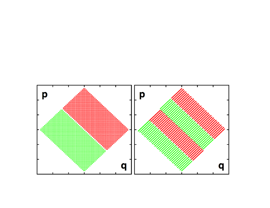
Figure 2: One iteration of the Baker Map is illustrated here for a grid of 1442 $(q,p)$ points. The square shown at the left is first squeezed twofold in the $q=p$ direction and stretched twofold in the perpendicular direction. After a cut along the $q=p$ line the two halves are joined together in the new arrangement shown at the right. The changed spacings of the points reflect the squeezing and stretching induced by the map.

III The Rotated Time-Reversible Baker Map

In the dynamical systems literature the discontinuous “Baker Map”, composed of area-preserving cutting and kneading operations, provides a simple illustration of “chaos”, the exponentially diverging growth induced by the mapping of small perturbations. The familiar “Cat Map” is another well-known discontinuous mapping of the unit square into itself. Both these map types illustrate Lyapunov instability, $\delta_{n+1}\propto\delta_{n}$ , where the proportionality constant exceeds unity, leading to divergence.

Many-to-one mappings, such as $x_{n+1}=\alpha x_{n}\ ;\ \alpha<1$ , in the presence of chaos are enough to produce the strange attractors associated with nonequilibrium steady states. Even one-to-one volume-preserving mappings, as in the simplest Baker Map above, are enough to generate Lyapunov unstable chaos. In the equilibrium Baker Map each half of a $2\times 2$ square is mapped from a $1\times 2$ rectangle to two $(1/2)\times 2$ disjoint rectangles. In order to follow our criterion for time reversibility – detailed in the next Section – we use a rotated version of the Baker Map, illustrated in Figure 2. The mapping is as follows :

if(q.lt.p) then
qnew = +1.25d00*q - 0.75d00*p + dsqrt(1.125d00)
pnew = -0.75d00*q + 1.25d00*p - dsqrt(0.125d00)
endif
if(q.gt.p) then
qnew = +1.25d00*q - 0.75d00*p - dsqrt(1.125d00)
pnew = -0.75d00*q + 1.25d00*p + dsqrt(0.125d00)
endif
The result of 100,000 iterations of this map is a near uniform covering of the $2\times 2$ square, as is shown in Figure 3.

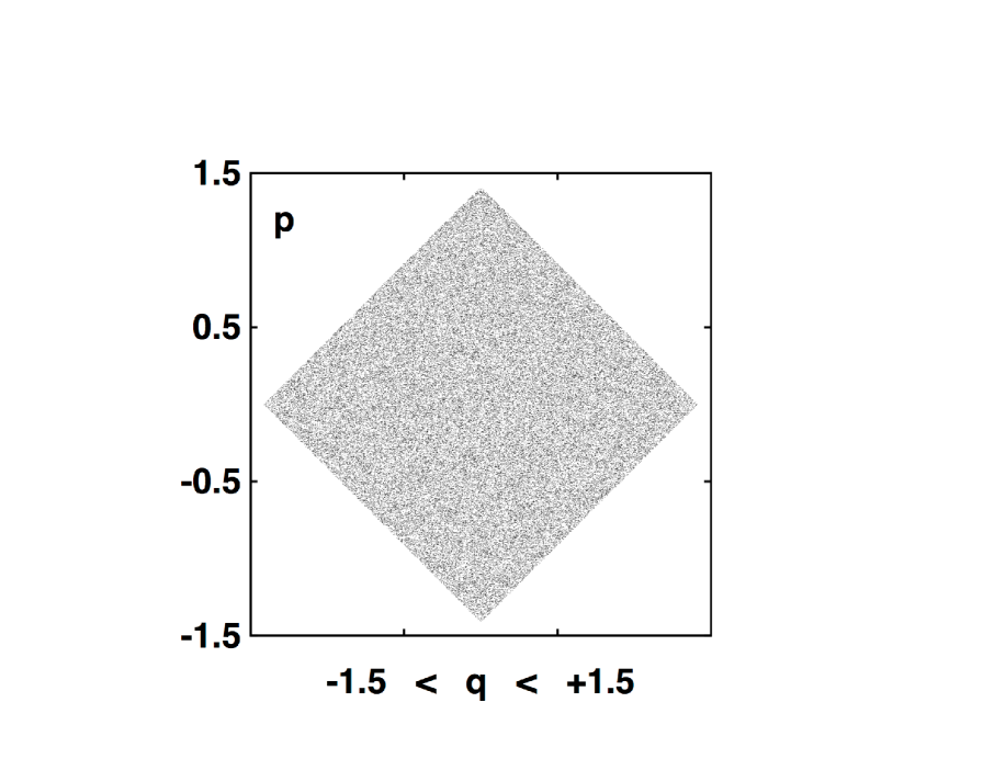
Figure 3: The uniform distribution of 100,000 iterates of the Baker Map with an initial point $(q,p)=(0.5,0.0)$ are plotted here. The uniform area conservation of the Map is analogous to the equilibrium phase-volume conservation described by Liouville’s Theorem.

The dissipative Baker Mapb4 ; b5 , with changes in area as well as shape, is a better model for nonequilibrium molecular dynamics and statistical mechanics. In those disciplines the phase-space density responds to heat transfer. In the oscillator example above the action of a heat reservoir with temperature $T(q)$ is represented by the time-reversible frictional force, $-\zeta[\ Ap+B(p^{3}/T)\ ]$ . The resulting change in comoving phase volume $\otimes$ follows from the continuity equation :

$$(\dot{\otimes}/\otimes)=(\partial\dot{q}/\partial q)+(\partial\dot{p}/\partial p)+(\partial\dot{\zeta}/\partial\zeta)=-\zeta[\ A+3B(p^{2}/T)\ ]\ .$$

The dissipative Baker Map is deterministic, time-reversible, and likewise produces mirror-image attractor-repellor multifractal pairs. These are the same qualities associated with nonequilibrium molecular dynamics algorithms ever since the early 1970s, though they passed unrecognized until the 1980s.b1

IV New Maps – Ian Snook Prize for 2015

The conducting oscillator is just one example of the deterministic, time-reversible flows that represent a nonequilibrium steady state with a chaotic multifractal attractor. The time-reversed state, with the momentum, friction coefficient, and the time all changed in sign, is an exactly similar mirror-image multifractal structure, an unstable zero-measure repellor. More complicated maps with these same properties can be constructed by concatenating time-symmetric combinations of reversible mappings $\{\ {\cal M}\ \}$ like

$${\cal M}_{1}{\cal M}_{2}{\cal M}_{3}{\cal M}_{4}{\cal M}_{3}{\cal M}_{2}{\cal M}_{1}\ .$$

where each of the mappings satisfies the time-reversibility criterion :

$$(q,p)={\cal TMTM}(q,p)\ ,$$

with the four operations performed from right to left. Here ${\cal T}$ indicates the time-reversal operation $(q,p)\longrightarrow(q,-p)$ . This reversibility criterion states that the sequence of four steps – [ 1 ] iterate forward; [ 2 ] reverse velocities; [ 3 ] iterate backward; [ 4 ] reverse velocities – returns to the original $(q,p)$ state. The simplest time-symmetric mappings satisfying this criterion are shears and reflections.b4 It is interesting to note that numerical implementations almost never return exactly to their initial state after the four-step sequence above. In fact the lack of an exact return is a ( somewhat misleading )b7 measure of algorithmic accuracyb8 .

The similarities between small-system dynamics and macroscopic dissipative behavior motivate the study of relatively simple flows and maps capable of generating the complexity associated with irreversible strange attractors. At the same time this complexity often exhibits a compelling beauty. The prototypical Cat and Baker maps are relatively simple, but their discontinuities are not at all representative of the attractor types shown in Figure 1 . The time is ripe for a fresh look at such problems.

The Snook Prize problem for 2015 is to formulate and analyze an interesting time-reversible ergodic map relevant to statistical mechanics, in two or three dimensions. It is desirable that the map generates a multifractal. Entries can be submitted to the authors, to the Los Alamos ar$\chi$iv, or to Computational Methods in Science and Technology. The author(s) of the most interesting entry received prior to 1 January 2016 will receive the Prize’s cash award of $500 US . The publisher of Computational Methods in Science and Technology ( cmst.eu ) has generously offered an Additional Prize award of $555.5$\dot{5}$ US subject to the Terms and Conditions published in CMST .

References

- (1) W. G. Hoover and C. G. Hoover, Simulation and Control of Chaotic Nonequilibrium Systems (World Scientific Publishers, Singapore, 2015) .
- (2) H. A. Posch and Wm. G. Hoover, “Time-Reversible Dissipative Attractors in Three and Four Phase-Space Dimensions”, Physical Review E 55, 6803-6810 (1997).
- (3) W. G. Hoover, J. C. Sprott, and C. G. Hoover, “Nonequilibrium Molecular Dynamics and Dynamical Systems theory for Small Systems with Time-Reversible Motion Equations”, Molecular Simulations ( in preparation, 2015 ) .
- (4) W. G. Hoover, O. Kum, and H. A. Posch, “Time-Reversible Dissipative Ergodic Maps”, Physical Review E 53, 2123-2129 (1996) .
- (5) J. Kumic̆ák, Irreversibility in a Simple Reversible Model”, Physical Review E 71, 016115 (2005) = ariv nlin/0510016 .
- (6) L. Ermann and D. L. Shepelyansky, “Arnold Cat Map, Ulam Method, and Time Reversal”, Physica D 241, 514-518 (2012) = ariv 1107.0437 .
- (7) W. G. Hoover and C. G. Hoover, “Comparison of Very Smooth Cell-Model Trajectories Using Five Symplectic and Two Runge-Kutta Integrators”, Computational Methods in Science and Technology 21(to appear, 2015) = ariv 1504.00620 .
- (8) D. Faranda, M. F. Mestre, and G. Turchetti, “Analysis of Roundoff Errors with Reversibility Test as a Dynamical Indicator”, International Journal of Bifurcation and Chaos 22, 1250215 (2012) = ariv 1205.3060 .