Coordinated Robot Navigation
via Hierarchical Clustering

Abstract

We introduce the use of hierarchical clustering for relaxed, deterministic coordination and control of multiple robots. Traditionally an unsupervised learning method, hierarchical clustering offers a formalism for identifying and representing spatially cohesive and segregated robot groups at different resolutions by relating the continuous space of configurations to the combinatorial space of trees. We formalize and exploit this relation, developing computationally effective reactive algorithms for navigating through the combinatorial space in concert with geometric realizations for a particular choice of hierarchical clustering method. These constructions yield computationally effective vector field planners for both hierarchically invariant as well as transitional navigation in the configuration space. We apply these methods to the centralized coordination and control of $n$ perfectly sensed and actuated Euclidean spheres in a $d$-dimensional ambient space (for arbitrary $n$ and $d$). Given a desired configuration supporting a desired hierarchy, we construct a hybrid controller which is quadratic in $n$ and algebraic in $d$ and prove that its execution brings all but a measure zero set of initial configurations to the desired goal with the guarantee of no collisions along the way.

I Introduction

Cooperative, coordinated action and sensing can promote efficiency, robustness, and flexibility in achieving complex tasks such as search and rescue, area exploration, surveillance and reconnaissance, and warehouse management [2]. Despite significant progress in the analysis of how local rules can yield such global spatiotemporal patterns [3, 4, 5], there has been strikingly less work on their specification. With few exceptions, the engineering literature on multirobot systems relies on task representations expressed in terms of rigidly imposed configurations — either by absolutely targeted positions, or relative distances — missing the intuitively substantial benefit of ignoring fine details of individual positioning, to focus control effort instead on the presumably far coarser properties of the collective pattern that matter. We seek a more relaxed means of specification that is sensitive to spatial distribution at multiple scales (as influencing the intensity of interactions among individuals and with their environment [6]) and the identities of neighbors (as determining the capabilities of heterogeneous teams [7]) while affording, nevertheless, a well-formed deterministic characterization of pattern.

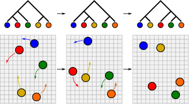
Figure 1: Moving from one spatial distribution to another is generally carried through rearrangements of robot groups (clusters) at different resolution corresponding to transitions between different cluster structures (hierarchies).

We are led to the notion of hierarchical clustering. We reinterpret this classical method for unsupervised learning [8] as a formalism for the specification and reactive implementation of collective mobility tasks expressed with respect to successively refined partitions of the agent set in a manner depicted in Fig. 1. There, we display three different configurations of five planar disks whose relative positions are specified by three distinct trees that represent differently nested clusters of relative proximity. The first configuration exhibits three distinct clusters at a resolution in the neighborhood of 2 units of distance: the red and the blue disks; the yellow and the orange disks; and the solitary green disk. At a coarser resolution, in the neighborhood of 4 units of distance, the green disk has merged into the subgroup including the red and the blue disks to comprise one of only two clusters discernible at this scale, the other formed by the orange and the yellow disks. It is intuitively clear that this hierarchical arrangement of subgroupings will persist under significant variations in the position of each individual disk. It is similarly clear that the second and third configurations (and significant variations in the positions of the individual disks of both) support the very differently nested clusters represented by the second and third trees, respectively. In this paper, we introduce a provably correct and computationally effective machinery for specifying, controlling invariantly to, and passing between such hierarchical clusterings at will.

As an illustration of its utility, we use this formalism to solve a specific instance of the reactive motion planning problem suggesting how the new “relaxed” hierarchy-sensitive layer of control can be merged with a task entailing a traditional rigidly specified goal pattern. Namely, for a collection of $n$ disk robots in $\mathbb{R}^{d}$ we presume that a target hierarchy has been specified along with a goal configuration that supports it, and that the robot group is controlled by a centralized source of perfect, instantaneous information about each agent’s position that can command exact instantaneous velocities for each disk. We present an algorithm resulting in a purely reactive hybrid dynamical system [9] guaranteed to bring the disk robots to both the hierarchical pattern as well as the rigidly specified instance from (almost) arbitrary initial conditions with no collisions of the disks along the way. Stated formally in Table III, the correctness of this algorithm is guaranteed by Theorem 1 whose proof appeals to the resolution of various constituent problems summarized in Table I. The construction is computationally effective: the number of discrete transitions grows in the worst case with the square of the number of robots, $n$; each successive discrete transition can be computed reactively (i.e., as a function of the present configuration) in time that grows linearly with the number of robots; and the formulae that define each successive vector field and guard condition are rational functions (defined by quotients of polynomials over the ambient space of degree less than $3$) entailing terms whose number grows quadratically with the number of robots.

TABLE I: Constituent Problems of Hierarchical Robot Navigation

Problem	Solution	Theorem	Description
1	Table IV	4	Hierarchy invariant vector field planner
2	Table V	5	Reactive navigation across hierarchies
3	Eqn.(39)	6	Cross-hierarchy geometric realization

This paper is organized as follows. We review in the next section the relevant background literature: first on reactive multirobot motion planning to relate the difficulty and importance of our sample problem to the state of the art in this field; next on the role of hierarchy in configuration spaces as explored both in biology and engineering. Because the notion of hierarchical clustering is a new abstraction for motion planning we devote Section III to a presentation of the key background technical ideas: first we review the relevant topological properties of configuration spaces; next the relevant topological properties of tree spaces; and, finally, prior work establishing properties of certain functions and relations between them. Because we feel that the specific motion planning problem we pose and solve represents a mere illustration of the larger value of this abstraction for multirobot systems we devote Section IV to a presentation of some of the more generic tools from which our particular construction is built: first we introduce the notion of hierarchy invariant navigation; next we discuss the combinatorial problem of hierarchy rearrangement as a graph navigation problem; and finally we interpret a subgraph of that combinatorial space as a “prepares” graph [10] for the hierarchy-invariant cover of configuration space. In Section V we pose and solve the specific motion planning problem using the concepts introduced in Section III and the tools introduced in Section IV. Section VI offers some numerical studies of the resulting algorithm. We conclude in Section VII with a summary of the major technical results that yield the specific contribution followed by some speculative remarks bearing on the likelihood that recent extensions of these ideas presently in progress [11] might afford a distributed reformulation, thus addressing the first (and better explored) remarkable biological inspiration for multirobot systems.

II Related Literature

II-A Multirobot Motion Planning

II-A1 Complexity

The intrinsic complexity of multibody configurations impedes computationally effective generalizations of single-robot motion planners [12, 13]. Coordinated motion planning of thick bodies in a compact space is computationally hard. For example, moving planar rectangular objects within a rectangular box is PSPACE-hard [14] and motion planning for finite planar disks in a polygonal environment is strongly NP-hard [15]. Even determining when and how the configuration space of noncolliding spheres in a unit box is connected entails an encounter with the ancient sphere packing problem [16]. Within the domain of reactive or vector field motion planning, it has proven deceptively hard to determine exactly this line of intractability. Consequently, this intrinsic complexity for coordinated vector field planners is generally mitigated by either assuming objects move in an unbounded (or sufficiently large) space [17, 18], as we do in Section V, or simply assuming conditions sufficient to guarantee connectivity between initial and goal configurations [19, 20]. On the other hand, more relaxed versions entailing (perhaps partially) homogeneous (unlabeled) specifications for interchangeable individuals have yielded computationally efficient planners in the recent literature [21, 22, 23, 24], and we suspect that the cluster hierarchy abstraction may be usefully applicable to such partially labeled settings.

II-A2 Reactive Multirobot Motion Planning

Since the problem of reactively navigating groups of disks was first introduced to robotics [25, 26], most research into vector field planners has embraced the navigation function paradigm [27]. A recent review of this two decade old literature is provided in [17], where a combination of intuitive and analytical results yields a nonsmooth centralized planner for achieving goal configurations specified up to rigid transformation. As noted in [17], the multirobot generalization of a single-agent navigation function is challenged by the violation of certain assumptions inherited from the original formulation [27]. One such assumption is that obstacles are “isolated” ( i.e. nonintersecting). In the multirobot case, every robot encounters others as mobile obstacles, and any collision between more than two robots breaks down the isolated obstacle assumption [17]. In some approaches, the departure from isolated interaction has been addressed by encoding all possible collision scenarios, yielding controllers with terms growing super-exponentially in the number of robots, even when the workspace is not compact [18]. In contrast, our recourse to the hierarchical representation of configurations affords a computational burden growing merely quadratically in the number of agents. In [19], the problem is circumvented by allowing critical points on the boundary (with no damage to the obstacle avoidance and convergence guarantees), but, as mentioned above, very conservative assumptions about the degree of separation between agents at the goal state are required. In contrast, our recourse to hierarchy allows us to handle arbitrary (non-intersecting) goal configurations, albeit our reliance upon the homotopy type of the underlying space presently precludes the consideration of a compact configuration space as formally allowed in [19].

Another limitation of navigation function approaches is the requirement of proper parameter tuning to eliminate local minima. Some effort has been given to automatic adaptation of this parameter [20], and, in principle, the original results of [27] guarantee that any monotone increasing scheme must eventually resolve the issue of local minima, however, this is numerically unfavorable (the Hessian of the resulting field becomes stiffer) and incurs substantial performance costs (transients must slow as the tuning parameter increases). In contrast, our recourse to hierarchy removes the need for any comparable tuning parameter.

Many of the concepts and some of the technical constructions we develop here were presented in preliminary form in the conference paper [1], building on the initial results of the conference paper [29]. This presentation gives a unified view of the detailed results (with some tutorial background) and contributes a major new extension by generalizing the construction of [1] from point particles to thickened disks of non-zero radius (necessitating a more involved version of the hierarchy invariant fields in Section V-B).

II-B The Use of Hierarchies as Organizational Models

II-B1 Hierarchy in Configuration Space

That a hierarchy of proximities might play a key role in computationally efficient coordinated motion planning had already been hinted at in early work on this problem [30, 31, 32]. Partial hierarchies that limit the combinatorial growth of complexity have been explicitly applied algorithmically to organize and simplify the systematic enumeration of cluster adjacencies in the configuration space [33]. Moreover, hierarchical discrete abstraction methods are successfully applied for scalable steering of a large number of robots as a group all together by controlling the group shape [34], and also find applications for congestion avoidance in swarm navigation [35]. While the utility of hierarchies and expressions for manipulating them are by no means new to this problem domain, we believe that the explicit formal connection [36] we exploit between the topology of configuration space [37] and the topology of tree space [38] through the hierarchical clustering relation [8] is entirely new.

II-B2 Hierarchy in Biology and Engineering

Biology offers spectacularly diverse examples of animal spatial organization ranging from self-sorting in cells [39], tissues and organs [40, 41], and groups of individuals [42, 43, 44] to more patterned teams [45, 46, 7, 47], all the way through strategic group formations in vertebrates [48, 49], mammals [50, 51, 52, 53], and primates [54, 55] hypothesized to increase efficacy in foraging [45, 46], hunting [54, 48, 50, 51], logistics and construction [7, 47], predator avoidance [56, 57], and even to stabilize whole ecologies [58] — all consequent upon the collective ability to target, track, and transform geometrically structured patterns of mutual location in response to environmental stimulus. These formations are remarkable for at least two reasons. First, their global structure seems to arise from local signaling and response amongst proximal individuals coupled to specific physical environments [59], in a manner that might be posited as a paradigm for generalized emergent intelligence [60]. Second, these formations appear to resist familiar rigid prescriptions governing absolute or relative location, instead giving wide latitude for individual autonomy and detailed positioning (intuitively, a necessity for negotiating fraught, highly dynamic interactions such as arise in, say, hunting [50, 52]), while, nevertheless, supporting the underlying coarse, deterministic “deep structure” as a dynamical invariant. It is this second remarkable attribute of biological swarms that inspires the present paper.

This profusion of pattern formation in biology has inspired a commensurate interest in robotics, yielding a growing literature on group coordination behaviors [61, 62, 63, 64] motivated by the intuition that the heterogeneous action and sensing abilities of a group of robots might enable a comparably diverse range of complex tasks beyond the capabilities of a single individual. For example, group coordination via splitting and merging behaviours creates effective strategies for obstacle avoidance [65], congestion control [35], shepherding [66], area exploration [66, 67], and maintaining persistent and coherent groups while adapting to the environment [64]. In almost all of the robotics work in this area, formation tasks are given based upon rigid specifications taking either the form of explicit formation or relative distance graphs, with few exceptions including the “shape” abstraction of [34] or applications in unknown environments such as area coverage and exploration [68]. Alternatively, hierarchical clustering offers an interesting means of ensemble task encoding and control; and it seems likely that the ability to specify organizational structure in the precise but flexible terms that hierarchy permits will add a useful tool to the robot motion planner’s toolkit.

TABLE II: Principal symbols used throughout this paper

$J$, $\mathrm{\mathbf{r}}$	Sets of labels and disk radii [III-A]
$\mathtt{Conf}\!\left(\mathbb{R}^{d}\!,J,\mathbf{r}\right)$	The conf. space of labelled, noncolliding disks (1)
$\mathcal{BT}_{J}$	The space of binary trees [III-B]
$\mathtt{HC}$	Hierarchical clustering [III-C]
$\mathtt{HC}_{\text{2-means}}$	Iterative 2-means clustering [V]
$\mathfrak{S}\!\left(\tau\right)$	The stratum of a tree, $\tau\in\mathcal{BT}_{J}$, (2)
$\mathtt{Portal}\left(\sigma,\tau\right)$	Portal configurations of a pair, $\left(\sigma,\tau\right)$, of trees (5)
${\mathtt{Port}}_{\sigma,\tau}$	Portal map [IV-A3]
$\mathcal{A}_{J}=\left(\mathcal{BT}_{J},\mathcal{E}_{\mathcal{A}}\right)$	The adjacency graph of trees [III-D]
$\mathcal{N}_{J}=\left(\mathcal{BT}_{J},\mathcal{E}_{\mathcal{N}}\right)$	The NNI-graph of trees [III-D]

III Hierarchical Abstraction

This section describes how we relate multirobot configurations to abstract cluster trees via hierarchical clustering methods and how we define connectivity in tree space.

III-A Configuration Space

For ease of exposing fundamental technical concepts, we restrict our attention to groups of Euclidean spheres in a $d$-dimensional ambient space, but many concepts introduced herein can be generalized to any metric space.

Given an index set, $J=[n]\>{\mathbf{:}\!=}\>\left\{1,\ldots,n\right\}\subset\mathbb{N}$, a heterogeneous multirobot configuration, $\mathrm{\mathbf{x}}=\left(\mathrm{x}_{j}\right)_{j\in J}$, is a labeled nonintersecting placement of $\left|J\right|=n$ distinct Euclidean spheres, where $i$th sphere is centered at $\mathrm{x}_{i}\in\mathbb{R}^{d}$ and has radius $r_{i}\geq 0$. We find it convenient to identify the configuration space [37] with the set of distinct labelings, i.e., the injective mappings of $J$ into $\mathbb{R}^{d}$, and, given a vector of nonnegative radii, $\mathbf{r}\>{\mathbf{:}\!=}\>\left(r_{j}\right)_{j\in J}\in\left(\mathbb{R}_{\geq 0}\right)^{J}$, we will find it convenient to denote our “thickened” subset of this configuration space as

$$\mathtt{Conf}\!\left(\mathbb{R}^{d}\!,J,\mathbf{r}\right)\!\!\>{\mathbf{:}\!=}\>\!\!\left\{\mathrm{\mathbf{x}}\!\in\!{(\mathbb{R}^{d})}^{\!J}\Big{|}\!\left\|\mathrm{x}_{i}\!-\!\mathrm{x}_{j}\right\|\!>\!r_{i}\!+\!r_{j},\forall i\!\neq\!j\!\in\!J\!\right\}\!\!,\!\!\!$$ (1)

where $\left\|.\right\|$ denotes the standard Euclidean norm on $\mathbb{R}^{d}$.

III-B Cluster Hierarchies

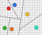
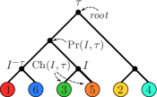
(a)	(b)

Figure 2: An illustration of (a) a heteregeneous configuration of unit disks in $\mathtt{Conf}\!\left(\mathbb{R}^{2},\left[6\right],\mathrm{\mathbf{1}}\right)$ and (b) its iterative 2-mean clustering [69] hierarchy $\tau$ in $\mathcal{BT}_{\left[6\right]}$, where the dashed lines in (a) depict the separating hyperplanes between clusters, and (b) illustrates hierarchical cluster relations: parent - $\mathrm{Pr}\left(I,\tau\right)$, children - $\mathrm{Ch}\left(I,\tau\right)$, and local complement (sibling) - ${I}^{-\tau}$ of cluster $I$ of the rooted binary tree, $\tau\in\mathcal{BT}_{\left[6\right]}$. An interior node is referred by its cluster, the list of leaves below it; for example, $I=\left\{3,5\right\}$. Accordingly the cluster set of $\tau$ is $\mathcal{C}\left(\tau\right)=\left\{\big{.}\!\left\{1\right\}\!,\left\{2\right\}\!,\ldots,\left\{6\right\}\!,\left\{1,6\right\}\!,\left\{3,5\right\}\!,\left\{2,4\right\}\!,\left\{1,3,5,6\right\}\!,\left\{1,2,3,4,5,6\right\}\!\right\}$.

A rooted semi-labelled tree $\tau$ over a fixed finite index set $J$, illustrated in Fig. 2, is a directed acyclic graph $G_{\tau}=\left(V_{\tau},E_{\tau}\right)$, whose leaves, vertices of degree one, are bijectively labeled by $J$ and interior vertices all have out-degree at least two; and all of whose edges in $E_{\tau}$ are directed away from a vertex designated to be the root [70]. A rooted tree with all interior vertices of out-degree two is said to be binary or, equivalently, non-degenerate, and all other trees are said to be degenerate. In this paper $\mathcal{BT}_{J}$ denotes the set of rooted nondegenerate trees over leaf set $J$.

A rooted semi-labelled tree $\tau$ uniquely determines (and henceforth will be interchangeably termed) a cluster hierarchy [71]. By definition, all vertices of $\tau$ can be reached from the root through a directed path in $\tau$. The cluster of a vertex $v\in V_{\tau}$ is defined to be the set of leaves reachable from $v$ by a directed path in $\tau$. Let $\mathcal{C}\left(\tau\right)$ denote the set of all vertex clusters of $\tau$.

For every cluster $I\in\mathcal{C}\left(\tau\right)$ we recall the standard notion of parent (cluster) $\mathrm{Pr}\left(I,\tau\right)$ and lists of children $\mathrm{Ch}\left(I,\tau\right)$, ancestors $\mathrm{Anc}\left(I,\tau\right)$ and descendants $\mathrm{Des}\left(I,\tau\right)$ of $I$ in $\tau$ — see [29] for explicit definitions of cluster relations. Additionally, we find it useful to define the local complement (sibling) of cluster $I\in\mathcal{C}\left(\tau\right)$ as ${I}^{-\tau}\>{\mathbf{:}\!=}\>\mathrm{Pr}\left(I,\tau\right)\setminus I$.

III-C Configuration Hierarchies

A hierarchical clustering $\mathtt{HC}\subset\mathtt{Conf}\!\left(\mathbb{R}^{d}\!,J,\mathbf{r}\right)\times\mathcal{BT}_{J}$ is a relation from the configuration space $\mathtt{Conf}\!\left(\mathbb{R}^{d}\!,J,\mathbf{r}\right)$ to the abstract space of binary hierarchies $\mathcal{BT}_{J}$ [8], an example depicted in Fig. 2. In this paper we will only be interested in clustering methods that can classify all possible configurations (i.e. for which $\mathtt{HC}$ assigns some tree to every configuration), and so we need:

Property 1

$\mathtt{HC}$ is a multi-function.

Most standard divisive and agglomerative hierarchical clustering methods exhibit this property, but generally fail to be functions because choices may be required between different but equally valid cluster splitting or merging decisions [8].

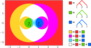
Figure 3: The Quotient Space $\mathtt{Conf}\!\left(\mathbb{C},\left[3\right],\mathrm{\mathbf{0}}\right)/\sim$, where for any $\mathrm{\mathbf{x}},\mathrm{\mathbf{y}}\in\mathtt{Conf}\!\left(\mathbb{C},\left[3\right],\mathrm{\mathbf{0}}\right)$, $\mathrm{\mathbf{x}}\sim\mathrm{\mathbf{y}}\Longleftrightarrow\frac{\mathrm{x}_{3}-\mathrm{x}_{1}}{\mathrm{x}_{2}-\mathrm{x}_{1}}=\frac{\mathrm{y}_{3}-\mathrm{y}_{1}}{\mathrm{y}_{2}-\mathrm{y}_{1}}$. Here, point particle configurations are quotiented out by translation, scale and rotation, and so $\mathrm{x}_{1}=0+0i$, $\mathrm{\mathbf{x}}_{2}=1+0i$ and $\mathrm{x}_{3}\in\mathbb{C}\setminus\left\{\mathrm{x}_{1},\mathrm{x}_{2}\right\}$. Regions are colored according the associated cluster hierarchies results from their iterative 2-mean clustering [69]. For instance, any configuration in the white region supports all hierarchies in $\mathcal{BT}_{\left[3\right]}$.

Given such an $\mathtt{HC}$, for any $\mathrm{\mathbf{x}}\in\mathtt{Conf}\!\left(\mathbb{R}^{d}\!,J,\mathbf{r}\right)$ and $\tau\in\mathcal{BT}_{J}$, we say $\mathrm{\mathbf{x}}$ supports $\tau$ if and only if $\left(\mathrm{\mathbf{x}},\tau\right)\in\mathtt{HC}$. The stratum associated with a binary hierarchy $\tau\in\mathcal{BT}_{J}$, denoted by $\mathfrak{S}\!\left(\tau\right)\subset\mathtt{Conf}\!\left(\mathbb{R}^{d}\!,J,\mathbf{r}\right)$, is the set of all configurations $\mathrm{\mathbf{x}}\in\mathtt{Conf}\!\left(\mathbb{R}^{d}\!,J,\mathbf{r}\right)$ supporting the same tree $\tau$ [29],

$$\mathfrak{S}\!\left(\tau\right)\>{\mathbf{:}\!=}\>\left\{\mathrm{\mathbf{x}}\in\mathtt{Conf}\!\left(\mathbb{R}^{d}\!,J,\mathbf{r}\right)\Big{|}\left(\mathrm{\mathbf{x}},\tau\right)\in\mathtt{HC}\right\},$$ (2)

and this yields a tree-indexed cover of the configuration space. For purposes of illustration, we depict in Fig. 3 the strata of $\mathtt{Conf}\!\left(\mathbb{C},\left[3\right],\mathrm{\mathbf{0}}\right)$ — a space that represents a group of three point particles on the complex plane.

The restriction to binary trees precludes combinatorial tree degeneracy [70] and we will avoid configuration degeneracy by imposing:

Property 2

Each stratum of $\mathtt{HC}$ includes an open subset of configurations, i.e. for every $\tau\in\mathcal{BT}_{J}$, $\mathring{\mathfrak{S}}\!\left(\tau\right)\neq\emptyset$.

Once again, most standard hierarchical clustering methods respect this assumption: they generally all agree (i.e. return the same result) and are robust to small perturbations of a configuration whenever all its clusters are compact and well separated [72].

Given any two multirobot configurations supporting the same cluster hierarchy, moving between them while maintaining the shared cluster hierarchy (introduced later as Problem 1) requires:

Property 3

Each stratum of $\mathtt{HC}$ is connected.

For an arbitrary clustering method this requirement is generally not trivial to show, but when configuration clusters of $\mathtt{HC}$ are linearly separable, one can characterize the topological shape of each stratum to verify this requirement, as we do in Section V-A.

Figure 4: An illustration of NNI moves between binary trees: each arrow is labeled by a source tree and an associated cluster defining the move.

III-D Graphs On Trees

After establishing the relation between multirobot configurations and cluster hierarchies, the final step of our proposed abstraction is to determine the connectivity of tree space.

Define the adjacency graph $\mathcal{A}_{J}=\left(\mathcal{BT}_{J},\mathcal{E}_{\mathcal{A}}\right)$ to be the 1-skeleton of the nerve [73] of the $\mathtt{Conf}\!\left(\mathbb{R}^{d}\!,J,\mathbf{r}\right)$-cover induced by $\mathtt{HC}$. That is to say, a pair of hierarchies, $\sigma,\tau\in\mathcal{BT}_{J}$, is connected with an edge in $\mathcal{E}_{\mathcal{A}}$ if and only if their strata intersect, $\mathfrak{S}\!\left(\sigma\right)\cap\mathfrak{S}\!\left(\tau\right)\neq\emptyset$. To enable navigation between structurally different multirobot configurations later (Problem 2), we need:

Property 4

The adjacency graph is connected.

Although the adjacency graph is a critical building block of our abstraction, as Fig. 3 anticipates, $\mathtt{HC}$ strata generally have complicated shapes, making it usually hard to compute the complete adjacency graph.

Fortunately, the computational biology literature [38] offers an alternative notion of adjacency that turns out to be both feasible and nicely compatible with our needs, yielding a computationally effective, connected subgraph of the adjacency graph, $\mathcal{A}_{J}$, as follows.

The Nearest Neighbor Interchange (NNI) move at a cluster $A\in\mathcal{C}\left(\sigma\right)$ on a binary hierarchy $\sigma\in\mathcal{BT}_{J}$, as illustrated in Fig. 4, swaps cluster $A$ with its parent’s sibling $C={\mathrm{Pr}\left(A,\sigma\right)}^{-\sigma}$ to yield another binary hierarchy $\tau\in\mathcal{BT}_{J}$ [74, 75]. Say that $\sigma,\tau\in\mathcal{BT}_{J}$ are NNI-adjacent if and only if one can be obtained from the other by a single NNI move. Moreover, define the NNI-graph $\mathcal{N}_{J}=\left(\mathcal{BT}_{J},\mathcal{E}_{\mathcal{N}}\right)$ to have vertex set $\mathcal{BT}_{J}$, with two trees connected by an edge in $\mathcal{E}_{\mathcal{N}}$ if and only if they are NNI-adjacent, see Fig. 5. An important contribution of this paper will be to show how the NNI-graph yields a computationally effective subgraph of the adjacency graph (Theorem 6).

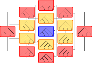
Figure 5: The NNI Graph: a graphical representation of the space of rooted binary trees, $\mathcal{BT}_{J}$, with NNI connectivity, where $J=\left[4\right]=\left\{1,2,3,4\right\}$.

IV Hierarchical Navigation Framework

Hierarchical abstraction introduced in Section III intrinsically suggests a two-level navigation strategy for coordinated motion design: (i) at the low-level perform finer adjustments on configurations using hierarchy preserving vector fields, (ii) and at the high-level resolve structural conflicts between configurations using a discrete transition policy in tree space; and the connection between these two levels are established through “portals” — open sets of configurations supporting two adjacent hierarchies. In this section we abstractly describe the generic components of our navigation framework and we show how they are put together.

IV-A Generic Components of Hierarchical Navigation

IV-A1 Hierarchy Preserving Navigation

For ease of exposition we restrict attention to first order (completely actuated single integrator) robot dynamics, and we will be interested in smooth closed loop feedback laws (or hybrid controllers composed from them) that result in complete flows,

$$\dot{\mathrm{\mathbf{x}}}=f\left(\mathrm{\mathbf{x}}\right),$$ (3)

where $f:\mathtt{Conf}\!\left(\mathbb{R}^{d}\!,J,\mathbf{r}\right)\rightarrow\left(\mathbb{R}^{d}\right)^{J}$ is a vector field over $\mathtt{Conf}\!\left(\mathbb{R}^{d}\!,J,\mathbf{r}\right)$ (1).

Denote by $\varphi^{t}$ the flow [79] on $\mathtt{Conf}\!\left(\mathbb{R}^{d}\!,J,\mathbf{r}\right)$ induced by the vector field $f$. For a choice of hierarchical clustering $\mathtt{HC}$, the class of hierarchy-invariant vector fields maintaining the robot group in a specified hierarchical arrangement of clusters, $\tau\in\mathcal{BT}_{J}$, is defined as [29],

$$\mathcal{F}_{\mathtt{HC}}(\tau)\!\>{\mathbf{:}\!=}\>\!\!\left\{\!f\!:\!\mathtt{Conf}\!\left(\mathbb{R}^{d}\!,J,\mathbf{r}\right)\!\!\rightarrow\!\left(\mathbb{R}^{d}\right)^{\!J}\!\Big{|}\varphi^{t}\!\left(\big{.}\mathfrak{S}\!\left(\tau\right)\!\right)\!\!\subset\!\mathfrak{S}\!\left(\tau\right)\!,t\!>\!0\!\right\}\!\!.\!\!\!$$ (4)

Hierarchy preserving navigation, the low-level component of our framework, uses the vector fields of $\mathcal{F}_{\mathtt{HC}}\left(\tau\right)$ to invariantly retract almost all of a stratum onto any designated goal configuration. Thus, we require the availability of such a construction, summarized as:

Problem 1

For any $\tau\in\mathcal{BT}_{J}$ and $\mathrm{\mathbf{y}}\in\mathfrak{S}\!\left(\tau\right)$ associated with $\mathtt{HC}$ construct a control policy, $f_{\tau,\mathrm{\mathbf{y}}}$, using the hierarchy invariant vector fields of $\mathcal{F}_{\mathtt{HC}}\left(\tau\right)$ whose closed loop asymptotically results in a retraction, $R_{\tau,\mathrm{\mathbf{y}}}$, of $\mathfrak{S}\!\left(\tau\right)$, possibly excluding a set of measure zero, onto $\left\{\mathrm{\mathbf{y}}\right\}$.

Key for purposes of the present application is the observation that any hierarchy-invariant field $f\in\mathcal{F}_{\mathtt{HC}}\left(\tau\right)$ must leave $\mathtt{Conf}\!\left(\mathbb{R}^{d}\!,J,\mathbf{r}\right)$ invariant as well, and thus avoids any self-collisions of the agents along the way.

IV-A2 Navigation in the Space of Binary Trees

Whereas the controlled deformation retraction, $R_{\tau,\mathrm{\mathbf{y}}}$, above generates paths “through” the strata, we will also want to navigate “across” them along the adjacency graph (which will be later in Section V replaced with the NNI-graph — a computationally efficient, connected subgraph). Thus, we further require a construction of a discrete feedback policy in $\mathcal{BT}_{J}$ that recursively generates paths in the adjacency graph toward any specified destination tree from all other trees in $\mathcal{BT}_{J}$ by reducing a “discrete Lyapunov function” relative to that destination, which we summarize as follows:

Problem 2

Given any $\tau\in\mathcal{BT}_{J}$ construct recursively a closed loop discrete dynamical system in the adjacency graph, taking the form of a deterministic discrete transition rule, $g_{\tau}$, with global attractor at $\tau$ endowed with a discrete Lyapunov function relative to the attractor $\tau$.

Such a recursively generated choice of next hierarchy will play the role of a discrete feedback policy used to define the reset map of our hybrid dynamical system.

IV-A3 Hierarchical Portals

Here, we relate the (combinatorial) topology of hierarchical clusters to the (continuous) topology of configurations by defining “portals” — open sets of configurations supporting two adjacent hierarchies.

Definition 1

The portal, $\mathtt{Portal}\left(\sigma,\tau\right)$, of a pair of hierarchies, $\sigma,\tau\in\mathcal{BT}_{J}$, is the set of all configurations supporting interior strata of both trees,

$$\mathtt{Portal}\left(\sigma,\tau\right)\>{\mathbf{:}\!=}\>\mathring{\mathfrak{S}}\!\left(\sigma\right)\cap\mathring{\mathfrak{S}}\!\left(\tau\right).$$ (5)

Namely, portals are geometric realizations in the configuration space of the edges of the adjacency graph on trees, see Fig. 3. To realize discrete transitions in tree space via hierarchy preserving navigation in the configuration space, we need a portal map that takes an edge of the adjacency graph, and returns a target configuration in the associated portal, summarized as:

Problem 3

Given an edge $\left(\sigma,\tau\right)\in\mathcal{E}_{\mathcal{A}}$ of the adjacency graph $\mathcal{A}_{J}=\left(\mathcal{BT}_{J},\mathcal{E}_{\mathcal{A}}\right)$, construct a geometric realization map ${\mathtt{Port}}_{\left(\sigma,\tau\right)}:\mathfrak{S}\!\left(\sigma\right)\rightarrow\mathtt{Portal}\left(\sigma,\tau\right)$ that takes a configuration supporting $\sigma$, and returns a target configuration supporting both trees $\sigma$ and $\tau$.

A portal map will serve the role of a dynamically computed “prepares graph” [10] for the sequentially composed local controllers whose correct recruitment solves the reactive coordinated motion planning problem (Theorem 1).

IV-B Specification and Correctness of the Hierarchical Navigation Control (HNC) Algorithm

Assume the selection of a goal configuration $\mathrm{\mathbf{y}}\in\mathfrak{S}\!\left(\tau\right)$ and a hierarchy $\tau\in\mathcal{BT}_{J}$ that $\mathrm{\mathbf{y}}$ supports. Now, given (almost) any initial configuration $\mathrm{\mathbf{x}}\in\mathfrak{S}\!\left(\sigma\right)$ for some hierarchy $\sigma\in\mathcal{BT}_{J}$ that $\mathrm{\mathbf{x}}$ supports, Table III presents the HNC algorithm.

TABLE III: The HNC Algorithm

For (almost) any initial $\mathrm{\mathbf{x}}\in\mathfrak{S}\!\left(\sigma\right)$ and $\sigma\in\mathcal{BT}_{J}$, and desired $\mathrm{\mathbf{y}}\in\mathfrak{S}\!\left(\tau\right)$ and $\tau\in\mathcal{BT}_{J}$, 1. (Hybrid Base Case) if $\mathrm{\mathbf{x}}\in\mathfrak{S}\!\left(\tau\right)$ then apply stratum-invariant dynamics, $f_{\tau,\mathrm{\mathbf{y}}}$ (Problem 1). 2. (Hybrid Recursive Step) else, (a) invoke the discrete transition rule $g_{\tau}$ (Problem 2) to propose an adjacent tree, $\gamma\in\mathcal{BT}_{J}$, with lowered discrete Lyapunov value. (b) Choose local configuration goal, $\mathrm{\mathbf{z}}:={\mathtt{Port}}_{\left(\sigma,\gamma\right)}\left(\mathrm{\mathbf{x}}\right)$ (Problem 3). (c) Apply the stratum-invariant continuous controller $f_{\sigma,\mathrm{\mathbf{z}}}$ (Problem 1). (d) If the trajectory enters $\mathfrak{S}\!\left(\tau\right)$ then go to step 1; else, the trajectory must enter $\mathfrak{S}\!\left(\gamma\right)$ in finite time in which case terminate $f_{\sigma,\mathrm{\mathbf{z}}}$, reassign $\sigma\leftarrow\gamma$, and go to step 2a).

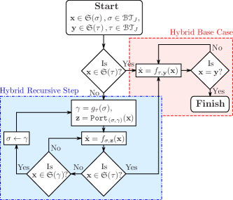
Figure 6: Flowchart of the hybrid vector field planner.

Theorem 1

The HNC Algorithm in Table III defines a hybrid dynamical system whose execution brings almost every initial configuration, $\mathrm{\mathbf{x}}\in\mathtt{Conf}\!\left(\mathbb{R}^{d},J\right)$, in finite time to an arbitrarily small neighborhood of $\mathrm{\mathbf{y}}\in\mathfrak{S}\!\left(\tau\right)$ with the guarantee of no collisions along the way.

• In the base case, 1) the conclusion follows directly from the construction of Problem 1: the flow $f_{\tau,\mathrm{\mathbf{y}}}$ keeps the state in $\mathfrak{S}\!\left(\tau\right)$, approaches a neighborhood of $\mathrm{\mathbf{y}}$ (which is an asymptotically stable equilibrium state for that flow) in finite time.

  In the inductive step, a) The NNI transition rule $g_{\tau}$ guarantees a decrement in the Lyapunov function after a transition from $\sigma$ to $\gamma$ (Problem 2), and a new local policy $f_{\sigma,\mathrm{\mathbf{z}}}$ is automatically deployed with a local goal configuration $\mathrm{\mathbf{z}}\in\mathtt{Portal}\left(\sigma,\gamma\right)$ found in b). Next, the flow $f_{\sigma,\mathrm{\mathbf{z}}}$ in c) is guaranteed to keep the state in $\mathfrak{S}\!\left(\sigma\right)$ and approach $\mathrm{\mathbf{z}}\in\mathtt{Portal}\left(\sigma,\gamma\right)$ asymptotically from almost all initial configurations. If the base case is not triggered in d), then the state enters arbitrarily small neighborhoods of $\mathrm{\mathbf{z}}$ and, hence, must eventually reach $\mathtt{Portal}\left(\sigma,\gamma\right)\subset\mathfrak{S}\!\left(\gamma\right)$ in finite time, triggering a return to 2a). Because the dynamical transitions $g_{\tau}$ initiated from any hierarchy in $\mathcal{BT}_{J}$ reaches $\tau$ in finite steps (Problem 2), it must eventually trigger the base case. ∎

V Hierarchical Navigation of Euclidean Spheres via Bisecting K-means Clustering

We now confine our attention to 2-means divisive hierarchical clustering [69], $\mathtt{HC}_{\text{2-means}}$, and demonstrate a construction of our hierarchical navigation framework for coordinated navigation of Euclidean spheres via $\mathtt{HC}_{\text{2-means}}$.

V-A Hierarchical Strata of $\mathtt{HC}_{\text{2-means}}$

Iterative 2-means clustering, $\mathtt{HC}_{\text{2-means}}$, is a divisive method that recursively constructs a cluster hierarchy of a configuration in a top-down fashion [69]. Briefly, this method splits each successive (partial) configuration by applying 2-means clustering, and successively continues with each subsplit until reaching singletons. By construction, complementary configuration clusters of $\mathtt{HC}_{\text{2-means}}$ are linearly separable by a hyperplane defined by the associated cluster centroids, as illustrated in Fig. 2; and the stratum of $\mathtt{HC}_{\text{2-means}}$ associated with a binary hierarchy $\tau\in\mathcal{BT}_{J}$ can be characterized by the intersection inverse images,

$$\mathfrak{S}\!\left(\tau\right) =\bigcap_{I\in\mathcal{C}\left(\tau\right)\setminus\left\{J\right\}}\bigcap_{i\in I}\eta_{i,I,\tau}^{-1}[0,\infty),$$ (6)

of the scalar valued “separation” function, $\eta_{i,I,\tau}:\mathtt{Conf}\!\left(\mathbb{R}^{d}\!,J,\mathbf{r}\right)\rightarrow\mathbb{R}$ [29] returning the distance of agent $i$ in cluster $I\in\mathcal{C}\left(\tau\right)\setminus\left\{J\right\}$ to the perpendicular bisector of the centroids of complementary clusters $I$ and ${I}^{-\tau}$:

$$\eta_{i,I,\tau}\left(\mathrm{\mathbf{x}}\right) \>{\mathbf{:}\!=}\>{\left(\big{.}\mathrm{x}_{i}-\mathrm{m}_{I,\tau}\left(\mathrm{\mathbf{x}}\right)\right)}^{\mathrm{T}}\frac{\mathrm{s}_{I,\tau}\left(\mathrm{\mathbf{x}}\right)}{\left\|\mathrm{s}_{I,\tau}\left(\mathrm{\mathbf{x}}\right)\right\|},$$ (7)

where the associated “cluster functions” of a partial configuration, $\mathrm{\mathbf{x}}|I=\left(\mathrm{x}_{i}\right)_{i\in I}$, are defined as

$$\mathrm{c}\left(\mathrm{\mathbf{x}}|I\right) \>{\mathbf{:}\!=}\>\frac{1}{|I|}\sum_{i\in I}\mathrm{x}_{i},$$ (8)

$$\mathrm{s}_{I,\tau}\left(\mathrm{\mathbf{x}}\right) \>{\mathbf{:}\!=}\>\mathrm{c}\left(\mathrm{\mathbf{x}}|I\right)-\mathrm{c}\left(\mathrm{\mathbf{x}}|{I}^{-\tau}\right),$$ (9)

$$\mathrm{m}_{I,\tau}\left(\mathrm{\mathbf{x}}\right) \>{\mathbf{:}\!=}\>\frac{\mathrm{c}\left(\mathrm{\mathbf{x}}|I\right)+\mathrm{c}\left(\mathrm{\mathbf{x}}|{I}^{-\tau}\right)}{2}.$$ (10)

We now follow [36] in defining terminology and expresssions leading to the characterization of the homotopy type of the stratum, $\mathfrak{S}\!\left(\tau\right),$ associated with a nondegenerate hierarchy. The proofs of our formal statements all follow the same pattern as established in [36], and we omit them to save space here.

Definition 2

A configuration $\mathrm{\mathbf{x}}\in\mathtt{Conf}\!\left(\mathbb{R}^{d}\!,J,\mathbf{r}\right)$ is narrow relative to the split, $\left\{I,J\setminus I\right\}$, if

$$\max_{A\in\left\{I,J\setminus I\right\}}r\left(\mathrm{\mathbf{x}}|A\right)\;<\;\frac{1}{2}\left\|\big{.}\mathrm{c}\left(\mathrm{\mathbf{x}}|I\right)-\mathrm{c}\left(\mathrm{\mathbf{x}}|J\setminus I\right)\right\|,$$ (11)

where the radius of a cluster, $A\subset J$, is defined to be

$$r\left(\mathrm{\mathbf{x}}|A\right):=\max_{a\in A}\left(\big{.}\left\|\mathrm{x}_{a}-\mathrm{c}\left(\mathrm{\mathbf{x}}|A\right)\right\|+r_{a}\right).$$ (12)

Say that $\mathrm{\mathbf{x}}\in\mathfrak{S}\!\left(\tau\right)$ is a standard configuration relative to the nondegenerate hierarchy, $\tau\in\mathcal{BT}_{J}$, if it is narrow relative to each local split, $\mathrm{Ch}\left(I,\tau\right)$, of every cluster, $I\in\mathcal{C}\left(\tau\right)$.

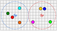
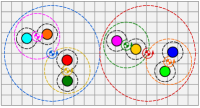
Figure 7: An illustration of (left) narrow and (right) standard disk configurations, where arrows and dashed circles indicate clusters that can be rigidly rotated around their centroids while preserving their clustering structures.

Proposition 1

If $\mathrm{\mathbf{x}}\in\mathfrak{S}\!\left(\tau\right)$ is a standard configuration then for each cluster, $I\in\mathcal{C}\left(\tau\right)$, any rigid rotation of the partial configuration, $\mathrm{\mathbf{x}}|I$, around its centroid, $\mathrm{c}\left(\mathrm{\mathbf{x}}|I\right)$, as illustrated in Fig. 7, preserves the supported hierarchy $\tau$.

Proposition 2

For any finite label set $J\subset\mathbb{N}$ and non-degenerate tree $\tau\in\mathcal{BT}_{J}$, there exists a strong deformation retraction

$$R_{\tau}:\mathfrak{S}\!\left(\tau\right)\times[0,1]\rightarrow\mathfrak{S}\!\left(\tau\right)$$ (13)

of $\mathfrak{S}\!\left(\tau\right)$ onto the subset of standard configurations of $\mathfrak{S}\!\left(\tau\right)$.

These two observations now yield the key insight reported in [36].

Theorem 2

The set of configurations $\mathrm{\mathbf{x}}\in\mathtt{Conf}\!\left(\mathbb{R}^{d}\!,J,\mathbf{r}\right)$ supporting a non-degenerate tree has the homotopy type of $(\mathbb{S}^{d-1})^{\left|J\right|-1}$.

To gain an intuitive appreciation, one can restate this result as follows: two configurations in $\mathfrak{S}\!\left(\tau\right)$ are topologically equivalent if and only if the corresponding separating hyperplane normals of configuration clusters are the same. Hence, navigation in a hierarchical stratum is carried out by aligning separating hyperplane normals, illustrated in Fig. 8; and using this geometric intuition, we construct in [29] a family of hierarchy preserving control policies for point particle configurations, and in the following we extend that construction to thickened disk configurations.

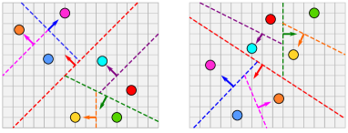
Figure 8: The topological shape of a hierarchical stratum intuitively suggests that global navigation in a hierarchical stratum is accomplished by aligning separating hyperplanes of configurations.

Theorem 3

Iterative 2-means clustering $\mathtt{HC}_{\text{2-means}}$ is a multi-function, and each of its stratum, $\mathfrak{S}\!\left(\tau\right)$ associated with $\tau\in\mathcal{BT}_{J}$, is connected and has an open interior.

• It is well known that $k$-means clustering is a multi-function generally yielding different $k$-partitions of any given data, and so is $\mathtt{HC}_{\text{2-means}}$ (Property 1)[8, 72]. Further, it follows from Definition 2 and Proposition 2 that standard configurations in $\mathfrak{S}\!\left(\tau\right)$ is open (Property 2), and Theorem 2 guarantees the connectedness of $\mathfrak{S}\!\left(\tau\right)$ (Property 3). ∎

V-B Hierarchy Preserving Navigation

We now introduce a recursively defined vector field for navigation in a hierarchical stratum and list its invariance and stability properties.

Suppose that some desired configuration, $\mathrm{\mathbf{y}}\in\mathfrak{S}\!\left(\tau\right)$ has been selected, supporting some desired nondegenerate tree, $\tau\in\mathcal{BT}_{J}$. Our dynamical planner takes the form of a centralized hybrid controller, $f_{\tau,\mathrm{\mathbf{y}}}:\mathfrak{S}\!\left(\tau\right)\rightarrow\left(\mathbb{R}^{d}\right)^{\left|J\right|}$, defining a hierarchy-invariant vector field whose flow in $\mathfrak{S}\!\left(\tau\right)$ yields the desired goal configuration, $\mathrm{\mathbf{y}}$, recursively defined according to logic presented in Table IV. Throughout this section, the tree $\tau$ and the goal configuration $\mathrm{\mathbf{y}}$ are fixed, and we therefore suppress all mention of these terms wherever convenient, in order to compress the notation. For example, for any $\mathrm{\mathbf{x}}\in\mathfrak{S}\!\left(\tau\right)$, $I\in\mathcal{C}\left(\tau\right)$ and $i\in I$ we use the shorthand $\eta_{i,I}\left(\mathrm{\mathbf{x}}\right)=\eta_{i,I,\tau}\left(\mathrm{\mathbf{x}}\right)$ (7), $\mathrm{s}_{I}\left(\mathrm{\mathbf{x}}\right)=\mathrm{s}_{I,\tau}\left(\mathrm{\mathbf{x}}\right)$ (9), $\mathrm{m}_{I}\left(\mathrm{\mathbf{x}}\right)=\mathrm{m}_{I,\tau}\left(\mathrm{\mathbf{x}}\right)$ (10) and so on.

TABLE IV: The Hierarchy-Preserving Navigation Vector Field

For any initial $\mathrm{\mathbf{x}}\in\mathfrak{S}\!\left(\tau\right)$ and desired $\mathrm{\mathbf{y}}\in\mathfrak{S}\!\left(\tau\right)$, supporting $\tau\in\mathcal{BT}_{J}$, the hierarchy preserving vector field, $f_{\tau,\mathrm{\mathbf{y}}}:\mathfrak{S}\!\left(\tau\right)\rightarrow\left(\mathbb{R}^{d}\right)^{J}$, $\displaystyle f_{\tau,\mathrm{\mathbf{y}}}\left(\mathrm{\mathbf{x}}\right)\>{\mathbf{:}\!=}\>\hat{f}_{\tau,\mathrm{\mathbf{y}}}\left(\mathrm{\mathbf{x}},\mathrm{\mathbf{0}},J\right),$ is recursively computed using the post-order traversal  of $\tau$ starting at the root cluster $J$ with the zero control input $\mathrm{\mathbf{0}}\in\left(\mathbb{R}^{d}\right)^{J}$ as follows: for any $\mathrm{\mathbf{u}}\in\left(\mathbb{R}^{d}\right)^{J}$ and $I\in\mathcal{C}\left(\tau\right)$, $\rotatebox{90.0}{Base Cases}\left\{\begin{array}[]{c}\\[1.42262pt] \\[1.42262pt] \\[1.42262pt] \\[1.42262pt] \end{array}\right.$ $\rotatebox{90.0}{Recursion}\left\{\begin{array}[]{c}\\[1.42262pt] \\[1.42262pt] \\[1.42262pt] \\[1.42262pt] \\[1.42262pt] \\[1.42262pt] \end{array}\right.$ 1. function $\hat{\mathrm{\mathbf{u}}}=\hat{f}_{\tau,\mathrm{\mathbf{y}}}\left(\mathrm{\mathbf{x}},\mathrm{\mathbf{u}},I\right)$ 2. if $\mathrm{\mathbf{x}}\in\mathcal{D}_{A}\left(I\right)$ (V-B), 3. $\hat{\mathrm{\mathbf{u}}}\leftarrow f_{A}\left(\mathrm{\mathbf{x}},\mathrm{\mathbf{u}},I\right)$ (16), 4. else if $\mathrm{\mathbf{x}}\not\in\mathcal{D}_{H}\left(I\right)$ (20), 5. $\hat{\mathrm{\mathbf{u}}}\leftarrow f_{S}\left(\mathrm{\mathbf{x}},\mathrm{\mathbf{u}},I\right)$ (26), 6. else 7. $\left\{I_{L},I_{R}\right\}\leftarrow\mathrm{Ch}\left(I,\tau\right)$, 8. $\hat{\mathrm{\mathbf{u}}}_{L}\leftarrow\hat{f}_{\tau,\mathrm{\mathbf{y}}}\left(\mathrm{\mathbf{x}},\mathrm{\mathbf{u}},I_{L}\right)$, 9. $\hat{\mathrm{\mathbf{u}}}_{R}\leftarrow\hat{f}_{\tau,\mathrm{\mathbf{y}}}\left(\mathrm{\mathbf{x}},\hat{\mathrm{\mathbf{u}}}_{L},I_{R}\right)$, 10. $\hat{\mathrm{\mathbf{u}}}\leftarrow f_{H}\left(\mathrm{\mathbf{x}},\hat{\mathrm{\mathbf{u}}}_{R},I\right)$ (21), 11. end 12. return $\hat{\mathrm{\mathbf{u}}}$ % Attracting Field % Split Separation Field % Recursion for Left Child % Recursion for Right Child % Split Preserving Field

In brief, the hierarchy invariant vector field $f_{\tau,\mathrm{\mathbf{y}}}$ recursively detects partial configurations whose separating hyperplanes are “sufficiently aligned” with the desired ones, as specified in (V-B) and illustrated in Fig. 9, and that can be directly moved towards the desired configurations, using a family of attracting fields $f_{A}$ (16), with no collisions along the way. Once the partial configurations associated with sibling clusters $I$ and ${I}^{-\tau}$ of $\tau$ are in the domains of their associated attracting fields, $f_{\tau,\mathrm{\mathbf{y}}}$ rotates these partial configurations while preserving the hierarchy so that their separating hyperplane is also asymptotically aligned. Hence, $f_{\tau,\mathrm{\mathbf{y}}}$ asymptotically aligns the separating hyperplanes of clusters of $\tau$ in a bottom-up fashion; and once the separating hyperplanes of all clusters of $\tau$ are “sufficiently aligned”, $f_{\tau,\mathrm{\mathbf{y}}}$ drives asymptotically each disk directly towards its desired location. We now present and motivate its constituent formulae as follows.

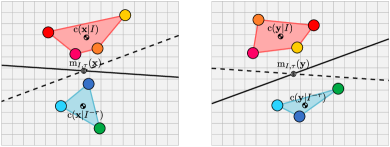
Figure 9: An illustration of “sufficiently aligned” separating hyperplanes of complementary clusters $I$ and ${I}^{-\tau}$ of $\tau$. Both of the current (left) and desired (right) partial configurations are linearly separable by each other’s separating hyperplane, and such an alignment condition needs to be satisfied at each level of the subtrees rooted at $I$ and ${I}^{-\tau}$ so that the partial configurations $\mathrm{\mathbf{x}}|I$ and $\mathrm{\mathbf{x}}|{I}^{-\tau}$ are steered by the associated attracting fields.

The hierarchy-invariant vector field, $f_{\tau,\mathrm{\mathbf{y}}}$, in Table IV.2) & IV.3) recursively detects partial configurations, $\mathrm{\mathbf{x}}|I$ associated with cluster $I\in\mathcal{C}\left(\tau\right)$, that can be safely driven toward the goal formation in $\mathfrak{S}\!\left(\tau\right)$ using a family of attracting controllers, $f_{A}:\mathfrak{S}\!\left(\tau\right)\times\left(\mathbb{R}^{d}\right)^{J}\times\mathcal{C}\left(\tau\right)\rightarrow\left(\mathbb{R}^{d}\right)^{J}$, defined in terms of the negated gradient field of $V\left(\mathrm{\mathbf{x}}\right)\>{\mathbf{:}\!=}\>\frac{1}{2}\left\|\mathrm{\mathbf{x}}-\mathrm{\mathbf{y}}\right\|_{2}^{2}$: for any $j\in J$,

$$f_{A}\left(\mathrm{\mathbf{x}},\mathrm{\mathbf{u}},I\right)_{j}\!\>{\mathbf{:}\!=}\>\!\left\{\begin{array}[]{@{}c@{}l}-(\mathrm{x}_{j}\!-\!\mathrm{y}_{j})&\text{, if }j\in I,\\ \mathrm{u}_{j}&\text{, else,}\end{array}\right.\!\!\!\!$$ (16)

where $\mathrm{\mathbf{u}}\in\left(\mathbb{R}^{d}\right)^{J}$ is a desired (velocity) control input specifying the motion of complementary cluster $J\setminus I$.

To avoid intra-cluster collisions along the way and preserve (local) clustering hierarchy, for any $I\in\mathcal{C}\left(\tau\right)$ the set of configurations in the domain of the attracting field, $f_{A}$, is restricted to

$$\mathcal{D}_{A}\!\left(I\right)\!\!\>{\mathbf{:}\!=}\>\!\!\left\{\Big{.}\right.\!\!\mathrm{\mathbf{x}}\!\in\!\mathfrak{S}\!\left(\tau\right)\!\Big{|}\, \mathcal{L}_{\overrightarrow{\mathrm{\mathbf{y}}}}{$\frac{1}{2}$}\left\|\mathrm{x}_{i}-\mathrm{x}_{j}\right\|^{2}\geq\left(r_{i}\!+\!r_{j}\right)^{2}\!\!,\,\forall i\!\neq\!\!j\!\in\!I\!,$$

$$\mathcal{L}_{\overrightarrow{\mathrm{\mathbf{y}}}}{\left(\mathrm{x}_{k}\!-\!\mathrm{m}_{K\!}\left(\mathrm{\mathbf{x}}\right)\!\right)\!}^{\mathrm{T}}\mathrm{s}_{K\!}\left(\mathrm{\mathbf{x}}\right)\!\geq\!0,\forall k\!\in\!K\!,K\!\in\!\mathrm{Des}\left(I,\tau\right)\!\!\left.\Big{.}\right\}\!\!,\!\!\!$$ (17)

where $\mathrm{Des}\left(I,\tau\right)$ is the set of descendants of $I$ in $\tau$. Here, $\mathcal{L}_{\overrightarrow{\mathrm{\mathbf{y}}}}f$ denotes the Lie derivative of a scalar-valued function $f$ along a constant vector field $\overrightarrow{\mathrm{\mathbf{y}}}$ which assigns the same vector $\mathrm{\mathbf{y}}$ to every point in its domain, and one can simply verify that

$$\mathcal{L}_{\overrightarrow{\mathrm{\mathbf{y}}}}{$\frac{1}{2}$}\left\|\mathrm{x}_{i}-\mathrm{x}_{j}\right\|^{2} ={\left(\mathrm{x}_{i}-\mathrm{x}_{j}\right)}^{\mathrm{T}}\left(\mathrm{y}_{i}-\mathrm{y}_{j}\right),$$ (18)

$$\mathcal{L}_{\overrightarrow{\mathrm{\mathbf{y}}}}{\left(\mathrm{x}_{k}\!-\!\mathrm{m}_{K\!}\left(\mathrm{\mathbf{x}}\right)\!\right)\!}^{\mathrm{T}}\mathrm{s}_{K\!}\left(\mathrm{\mathbf{x}}\right) ={\left(\mathrm{y}_{k}\!-\!\mathrm{m}_{K\!}\left(\mathrm{\mathbf{y}}\right)\!\right)\!}^{\mathrm{T}}\mathrm{s}_{K\!}\left(\mathrm{\mathbf{x}}\right)$$

$$\hskip 25.60747pt+{\left(\mathrm{x}_{k}\!-\!\mathrm{m}_{K\!}\left(\mathrm{\mathbf{x}}\right)\!\right)\!}^{\mathrm{T}}\mathrm{s}_{K\!}\left(\mathrm{\mathbf{y}}\right)\!.\!\!$$ (19)

Note that (18) quantifies the safety of a resulting trajectory of $f_{A}$, and to avoid collision between any pair of disks, $i$ and $j$, (18) should be no less than the square of sum of their radii, $\left(r_{i}+r_{j}\right)^{2}$, as required in (V-B); and (19) quantifies the preservation of (local) clustering hierarchy and should be nonnegative for hierarchy invariance. Also observe that since a singleton cluster contains no pair of distinct indices, and has an empty set of descendants, the predicate in (V-B) is always true for these “leaf” node cases and we have $\mathcal{D}_{A}\left(I\right)=\mathfrak{S}\!\left(\tau\right)$ for any singleton cluster $I\in\mathcal{C}\left(\tau\right)$. Further, one can simply verify that $\mathrm{\mathbf{y}}\in\mathcal{D}_{A}\left(I\right)$ for any $I\in\mathcal{C}\left(\tau\right)$.

If a partial configuration, $\mathrm{\mathbf{x}}|I$, is not contained in the domain of the associated attracting field, i.e. $\mathrm{\mathbf{x}}\not\in\mathcal{D}_{A}\left(I\right)$, to avoid inter-cluster collisions the failure of the condition in Table IV.4) ensures sibling clusters, $\mathrm{Ch}\left(I,\tau\right)$, will be separated by a certain distance, specified as:

$$\mathcal{D}_{H}\!\left(I\right)\!\!\>{\mathbf{:}\!=}\>\!\!\left\{\mathrm{\mathbf{x}}\!\in\!\mathfrak{S}\!\left(\tau\right)\!\Big{|}\eta_{k,K\!}\left(\mathrm{\mathbf{x}}\right)\!\geq\!r_{k}\!\!+\!\alpha,\forall k\!\in\!K,K\!\in\!\mathrm{Ch}\left(I,\tau\right)\!\right\}\!,\!\!\!$$ (20)

where $\eta_{k,K\!}\left(\mathrm{\mathbf{x}}\right)$ (7) returns the perpendicular distance of $k$th agent to the separating hyperplane of cluster $K\in\mathcal{C}\left(\tau\right)$, and $\alpha>0$ is a safety margin guaranteeing that the clearance between any pair of disks in complementary clusters, $\mathrm{Ch}\left(I,\tau\right)$, is at least $2\alpha$ units. Observe that $\mathcal{D}_{H}\left(I\right)=\mathfrak{S}\!\left(\tau\right)$ for any singleton cluster $I\in\mathcal{C}\left(\tau\right)$ because such leaf clusters of a binary tree have no children, i.e. $\mathrm{Ch}\left(I,\tau\right)=\emptyset$.

While the disks move in $\mathcal{D}_{H}\left(I\right)$ based on a desired control (velocity) input $\mathrm{\mathbf{u}}\in\left(\mathbb{R}^{d}\right)^{J}$, Table IV.10) guarantees the maintenance of the safety margin between children clusters $\mathrm{Ch}\left(I,\tau\right)$ by employing an additive repulsive field, $f_{H}:\mathfrak{S}\!\left(\tau\right)\times\left(\mathbb{R}^{d}\right)^{J}\times\mathcal{C}\left(\tau\right)\rightarrow\left(\mathbb{R}^{d}\right)^{J}$, as follows:

$$f_{H}\left(\mathrm{\mathbf{x}},\mathrm{\mathbf{u}},I\right)_{j}\>{\mathbf{:}\!=}\>\mathrm{u}_{j}+2\alpha_{I}\left(\mathrm{\mathbf{x}},\mathrm{\mathbf{u}}\right)\frac{\left|{K}^{-\tau}\right|}{\left|I\right|}\frac{\mathrm{s}_{K\!}\left(\mathrm{\mathbf{x}}\right)}{\left\|\mathrm{s}_{K\!}\left(\mathrm{\mathbf{x}}\right)\right\|},\!\!$$ (21)

for all $j\!\in\!K$ and $K\!\in\!\mathrm{Ch}\left(I,\tau\right)$; otherwise, $f_{H}\left(\mathrm{\mathbf{x}},\mathrm{\mathbf{u}},I\right)_{j}\!\>{\mathbf{:}\!=}\>\mathrm{u}_{j}$, where $\alpha_{I}\left(\mathrm{\mathbf{x}},\mathrm{\mathbf{u}}\right)$ is a scalar valued function describing the strength of the repulsive field,

$$\alpha_{I}\left(\mathrm{\mathbf{x}},\mathrm{\mathbf{u}}\right)\!\>{\mathbf{:}\!=}\>\!\max_{\begin{subarray}{c}k\in K\\ K\in\mathrm{Ch}\left(I,\tau\right)\end{subarray}}\phi_{k,K\!}\left(\mathrm{\mathbf{x}}\right)\cdot\psi_{k,K\!}\left(\mathrm{\mathbf{x}},\mathrm{\mathbf{u}}\right).$$ (22)

Here, for each individual $k$ in cluster $K\in\mathrm{Ch}\left(I,\tau\right)$, $\phi_{k,K}\left(\mathrm{\mathbf{x}}\right)$ is exponential damping on the repulsion strength $\psi_{k,K}\left(\mathrm{\mathbf{x}},\mathrm{\mathbf{y}}\right)$, in which the amplitude envelop exponentially decays to zero after a certain safety margin $\beta>\alpha$,

$$\phi_{k,K\!}\left(\mathrm{\mathbf{x}}\right) \!\>{\mathbf{:}\!=}\>\!\max\left(\frac{{e^{-\left(\eta_{k,K}\left(\mathrm{\mathbf{x}}\right)-r_{k}-\alpha\right)}\!-\!e^{-\left(\beta-\alpha\right)}}}{{1-e^{-\left(\beta-\alpha\right)}}},0\!\right)\!\!,$$ (23)

$$\psi_{k,K\!}\left(\mathrm{\mathbf{x}},\mathrm{\mathbf{u}}\right) \!\>{\mathbf{:}\!=}\>\!\max\left(\!\!\!\Big{.}-\!\!\left(\big{.}\eta_{k,K\!\!}\left(\mathrm{\mathbf{x}}\right)\!-\!r_{k}\!-\!\alpha\right)\!\!-\!\mathcal{L}_{\overrightarrow{\mathrm{\mathbf{u}}}}\eta_{k,K\!\!}\left(\mathrm{\mathbf{x}}\right)\!,0\!\right)\!\!,\!\!\!\!$$ (24)

where

$$\mathcal{L}_{\overrightarrow{\mathrm{\mathbf{u}}}}\eta_{k,K\!}\left(\mathrm{\mathbf{x}}\right) =\frac{{\left(\mathrm{u}_{k}\!-\!\mathrm{m}_{K\!}\left(\mathrm{\mathbf{u}}\right)\!\right)\!}^{\mathrm{T}}\mathrm{s}_{K\!}\left(\mathrm{\mathbf{x}}\right)\!+\!{\left(\mathrm{x}_{k}\!-\!\mathrm{m}_{K\!}\left(\mathrm{\mathbf{x}}\right)\!\right)\!}^{\mathrm{T}}\mathrm{s}_{K\!}\left(\mathrm{\mathbf{u}}\right)}{\left\|\mathrm{s}_{K\!}\left(\mathrm{\mathbf{x}}\right)\right\|}$$

$$\hskip 42.67912pt-\eta_{k,K\!}\left(\mathrm{\mathbf{x}}\right)\frac{{\mathrm{s}_{K\!}\left(\mathrm{\mathbf{x}}\right)\!}^{\mathrm{T}}\mathrm{s}_{K\!}\left(\mathrm{\mathbf{u}}\right)}{\left\|\mathrm{s}_{K\!}\left(\mathrm{\mathbf{x}}\right)\right\|^{2}}.$$ (25)

Note that $f_{H}\left(\mathrm{\mathbf{x}},\mathrm{\mathbf{u}},I\right)$ is well defined for any singleton cluster $I\in\mathcal{C}\left(\tau\right)$ and is equal to the identity map, i.e. $f_{H}\left(\mathrm{\mathbf{x}},\mathrm{\mathbf{u}},I\right)=\mathrm{\mathbf{u}}$, since $\mathrm{Ch}\left(I,\tau\right)=\emptyset$; and also observe that $f_{H}\left(\mathrm{\mathbf{x}},\mathrm{\mathbf{u}},I\right)=\mathrm{\mathbf{u}}$ for any $I\in\mathcal{C}\left(\tau\right)$ if the complementary clusters $\mathrm{Ch}\left(I,\tau\right)$ are well-separated, i.e. $\eta_{k,K}\left(\mathrm{\mathbf{x}}\right)\geq r_{k}+\beta$ for all $k\in K$ and $K\in\mathrm{Ch}\left(I,\tau\right)$. The latter is important to avoid the “finite escape time” phenomenon (Proposition 14).

Finally, Table IV.5) guarantees that if a partial configuration is neither in the domain of the attracting field nor are its children clusters, $\mathrm{Ch}\left(I,\tau\right)$, properly separated, i.e. $\mathrm{\mathbf{x}}\not\in\mathcal{D}_{A}\left(I\right)\cup\mathcal{D}_{H}\left(I\right)$, then the complementary clusters are driven apart using another repulsive field, $f_{S}:\mathfrak{S}\!\left(\tau\right)\times\left(\mathbb{R}^{d}\right)^{J}\times\mathcal{C}\left(\tau\right)\rightarrow\left(\mathbb{R}^{d}\right)^{J}$, until asymptotically establishing a certain safety margin $\beta>\alpha$:

$$f_{S}\left(\mathrm{\mathbf{x}},\mathrm{\mathbf{u}},I\right)_{j}\!\>{\mathbf{:}\!=}\>\!-\mathrm{c}\left(\mathrm{\mathbf{x}}\!-\!\mathrm{\mathbf{y}}|I\right)+2\beta_{I\!}\left(\mathrm{\mathbf{x}}\right)\!\frac{\left|{K}^{-\tau}\right|}{\left|I\right|}\frac{\mathrm{s}_{K\!}\left(\mathrm{\mathbf{x}}\right)}{\left\|\mathrm{s}_{K\!}\left(\mathrm{\mathbf{x}}\right)\right\|},\!\!\!$$ (26)

for all $j\!\in\!K$ and $K\!\in\!\mathrm{Ch}\left(I,\tau\right)$; otherwise, $f_{S}\left(\mathrm{\mathbf{x}},\mathrm{\mathbf{u}},I\right)_{j}\!\>{\mathbf{:}\!=}\>\mathrm{u}_{j}$, where the magnitude, $\beta_{I}\left(\mathrm{\mathbf{x}}\right)$, of repulsion between complementary clusters $\mathrm{Ch}\left(I,\tau\right)$ is given by

$$\beta_{I}\left(\mathrm{\mathbf{x}}\right)\>{\mathbf{:}\!=}\>\max_{\begin{subarray}{c}k\in K\\ K\in\mathrm{Ch}\left(I,\tau\right)\end{subarray}}\!\!\max\left(\big{.}\!-\left(\big{.}\eta_{k,K}\left(\mathrm{\mathbf{x}}\right)\!-\!r_{k}\!-\!\beta\right)\!,0\right)\!.\!$$ (27)

For completeness, we set $f_{S}\left(\mathrm{\mathbf{x}},\mathrm{\mathbf{u}},I\right)=f_{A}\left(\mathrm{\mathbf{x}},\mathrm{\mathbf{u}},I\right)$ for any singleton cluster $I\in\mathcal{C}\left(\tau\right)$.

We summarize the properties of this construction as follows:

Theorem 4

The recursion of Table IV results in a well-defined function $f_{\tau,\mathrm{\mathbf{y}}}:\mathfrak{S}\!\left(\tau\right)\rightarrow\left(\mathbb{R}^{d}\right)^{J}$ that can be computed in $\mathrm{O}\left(\left|J\right|^{2}\right)$ time for any $\mathrm{\mathbf{x}}\in\mathfrak{S}\!\left(\tau\right)$. For all $\tau\in\mathcal{BT}_{J}$, the stratum, $\mathfrak{S}\!\left(\tau\right)$ is positive invariant and any $\mathrm{\mathbf{y}}\in\mathfrak{S}\!\left(\tau\right)$ is an asymptotically stable equilibrium point of a continuous piecewise smooth flow arising from $f_{\tau,\mathrm{\mathbf{y}}}$ whose basin of attraction includes all of $\mathfrak{S}\!\left(\tau\right)$ with the exception of an empty interior set.

• These results are proven in Appendix A according to the following plan. Proposition 3 establishes that the recursion in Table IV indeed results in a function computable in quadratic time. The invariance, stability, and continuous flow generating properties of $f_{\tau,\mathrm{\mathbf{y}}}$ are shown using an equivalent system model within the sequential composition framework [10], as follows. Table VII defines a new recursion shown in Proposition 4 to result in a family of continuous and piecewise smooth vector fields. Proposition 5 asserts that the family of domains associated with these fields (63) defines a (finite) open cover of $\mathfrak{S}\!\left(\tau\right)$ relative to which a selection function (Table VIII) induces a partition of that stratum. Proposition 6 demonstrates that the composition of the covering vector field family with the output of this partitioning function yields a new function that coincides exactly with the original control field defined in Table IV. Finally, Proposition 14, Proposition 13 and Proposition 15 demonstrate, respectively, the flow, positive invariance and stability properties of $f_{\tau,\mathrm{\mathbf{y}}}$, which are inherited from the flow, invariance and stability properties (Proposition 10, Proposition 9 and Proposition 11, respectively) of substratum policies executed over a strictly decreasing finite prepares graph (Proposition 7) via their nondegenerately, real-time executed (Proposition 12) sequential composition. ∎

V-C Navigation in the Space of Binary Trees

In principle, navigation in the adjacency graph of trees (Problem 2) is a trivial matter since the number of trees over a finite set of leaves is finite. However, in practice, the cardinality of trees grows super exponentially [70],

$$\left|\mathcal{BT}_{J}\right| =(2\left|J\right|-3)!!=(2\left|J\right|-3)(2\left|J\right|-5)\ldots 3,$$ (28)

for $\left|J\right|\geq 2$. Hence standard graph search algorithms, like the A* or Dijkstra’s algorithm [81], become rapidly impracticable. In particular, computing the shortest path (geodesic) in the NNI-graph, a regular subgraph of the adjacency graph (Theorem 6), is NP-complete [84].

Alternatively, we have recently developed in [85] an efficient recursive procedure for navigating in the NNI graph $\mathcal{N}_{J}=\left(\mathcal{BT}_{J},\mathcal{E}_{\mathcal{N}}\right)$ towards any given binary tree $\tau\in\mathcal{BT}_{J}$, taking the form of an abstract discrete dynamical system as follows:

$$\sigma^{k+1} =\text{NNI}\left(\big{.}\sigma^{k},G^{k}\right),$$ (29a)

$$G^{k} =\mathrm{\mathbf{u}}_{\tau}(\sigma^{k}),$$ (29b)

where $\text{NNI}\left(\sigma^{k},G^{k}\right)$ denotes the NNI move on $\sigma^{k}$ at cluster $G^{k}\in\mathcal{C}\left(\tau\right)$, illustrated in Fig. 4, and $\mathrm{\mathbf{u}}_{\tau}$ is our NNI control policy returning an NNI move as summarised in Table V. Abusing notation, we shall denote the closed-loop dynamical system as

$$\sigma^{k+1}=g_{\tau}\left(\sigma^{k}\right)\>{\mathbf{:}\!=}\>\left(\text{NNI}\circ\mathrm{\mathbf{u}}\right)\left(\sigma^{k}\right).$$ (30)

TABLE V: The NNI Control Law

To navigate from an arbitrary hierarchy $\sigma\in\mathcal{BT}_{J}$ towards any selected desired hierarchy $\tau\in\mathcal{BT}_{J}$ in the NNI-graph, the NNI control policy $\mathrm{\mathbf{u}}_{\tau}$ returns an NNI move on $\sigma$ at a cluster $G\in\mathcal{C}\left(\sigma\right)$, as follows: 1. If $\sigma=\tau$, then just return the identity move, $G=\emptyset$. 2. Otherwise, (a) Select a common cluster $K\in\mathcal{C}\left(\sigma\right)\cap\mathcal{C}\left(\tau\right)$ with $\mathrm{Ch}\left(K,\sigma\right)\neq\mathrm{Ch}\left(K,\tau\right)$, and let $\left\{K_{L},K_{R}\right\}=\mathrm{Ch}\left(K,\tau\right)$. (b) Find a nonsingleton cluster $I\in\mathcal{C}\left(\sigma\right)$ with children $\left\{I_{L},I_{R}\right\}=\mathrm{Ch}\left(I,\sigma\right)$ satisfying $I_{L}\subseteq K_{L}$ and $I_{R}\subseteq K_{R}$. (c) Return a proper NNI navigation move on $\sigma$ at grandchild $G\in\mathrm{Ch}\left(I,\sigma\right)$ selected as follows: i. If ${I}^{-\sigma}\subset K_{L}$ , then return $G=I_{R}$. ii. Else if ${I}^{-\sigma}\subset K_{R}$ , then return $G=I_{L}$. iii. Otherwise , return an arbitrary NNI move at a child of $I$ in $\sigma$; for example, $G=I_{L}$.

The NNI control law endows the NNI-graph with a directed edge structure whose paths all lead to $\tau$, and whose longest path (from the furthest possible initial hierarchy, $\sigma\in\mathcal{BT}_{J}$) is tightly bounded by $\frac{1}{2}\left(\left|J\right|-1\right)\left(\left|J\right|-2\right)$ for $\left|J\right|\geq 2$. Given such a goal we show in [85] that the cost of computing an appropriate NNI move from any other $\sigma\in\mathcal{BT}_{J}$ toward an adjacent tree at a lower value of a “discrete Lyapunov function” relative to that destination is $\mathrm{O}\left(\left|J\right|\right)$. We summarize such important properties of our NNI navigation algorithm as:

Theorem 5 ([85] )

The NNI control law $\mathrm{u}_{\tau}$ (Table V) recursively defines a closed loop discrete dynamical system (30) in the NNI-graph, taking the form of a discrete transition rule, $g_{\tau}$, with global attractor at $\tau$ and longest trajectory of length $\mathrm{O}\left(\left|J\right|^{2}\!\right)$ endowed with a discrete Lyapunov function relative to which computing a descent direction from any $\sigma\in\mathcal{BT}_{J}$ requires a computation of time $\mathrm{O}\left(\left|J\right|\right)$.

V-D Portal Transformations

We now turn attention to construction of the crucial portal map that effects the geometric realization of the NNI-graph as required for Problem 3; and herein we extend our recent construction of the realization function, ${\mathtt{Port}}$, in [1] for point particle configurations to thickened disk configurations.

Throughout this section, the trees $\sigma,\tau\in\mathcal{BT}_{J}$ are NNI-adjacent (as defined in Section III-D) and fixed, and we therefore take the liberty of suppressing all mention of these trees wherever convenient, for the sake of simplifying the presentation of our equations.

Since the trees $\sigma,\tau$ are NNI-adjacent, we may apply Lemma 1 from [85] to find common disjoint clusters $A,B,C$ such that $\left\{A\cup B\right\}=\mathcal{C}\left(\sigma\right)\setminus\mathcal{C}\left(\tau\right)$ and $\left\{B\cup C\right\}=\mathcal{C}\left(\tau\right)\setminus\mathcal{C}\left(\sigma\right)$. Note that the triplet $\left\{A,B,C\right\}$ of the pair $\;\left(\sigma,\tau\right)$ is unique. We call $\left\{A,B,C\right\}$ the NNI-triplet of the pair $\left(\sigma,\tau\right)$. Since $\sigma$ and $\tau$ are fixed throughout this section, so will be $A,B,C$ and $P:=A\cup B\cup C$.

In the construction of the portal map, ${\mathtt{Port}}$ (39), we restrict our attention to the portal configurations with a certain symmetry property, defined as:

Definition 3 (​​[1])

We call $\mathrm{\mathbf{x}}\in\left(\mathbb{R}^{d}\right)^{J}$ a symmetric configuration associated with $\left(\sigma,\tau\right)$ if centroids of partial configurations $\mathrm{\mathbf{x}}|A$, $\mathrm{\mathbf{x}}|B$ and $\mathrm{\mathbf{x}}|C$ form an equilateral triangle, as illustrated in Fig. 10. The set of all symmetric configurations with respect to $\left(\sigma,\tau\right)$ is denoted $\mathtt{Sym}\left(\sigma,\tau\right)$.

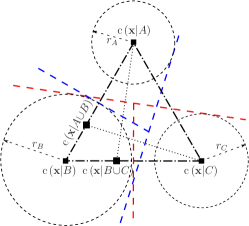
Figure 10: An illustration of a symmetric configuration $\mathrm{\mathbf{x}}\in\mathtt{Sym}\left(\sigma,\tau\right)$, where the consensus ball $B_{Q}\left(\mathrm{\mathbf{x}}\right)$ of partial configuration of cluster $Q\in\left\{A,B,C\right\}$ has a positive radius.

An important observation about the symmetric configurations is:

Lemma 1 (​​[1])

Let $\mathrm{\mathbf{x}}\in\mathfrak{S}\!\left(\sigma\right)$ be a symmetric configuration in $\mathtt{Sym}\left(\sigma,\tau\right)$. If each partial configuration $\mathrm{\mathbf{x}}|Q$ of cluster $Q\in\left\{A,B,C\right\}$ is contained in the associated “consensus” ball $B_{Q}\left(\mathrm{\mathbf{x}}\right)$ — an open ball centered at $\mathrm{c}\left(\mathrm{\mathbf{x}}|Q\right)$ with radius

$$r_{Q}\left(\mathrm{\mathbf{x}}\right) \!\>{\mathbf{:}\!=}\>\!\min_{\begin{subarray}{c}\gamma\;\in\;\left(\sigma,\tau\right)\\ D\in\left\{Q,\mathrm{Pr}\left(Q,\gamma\right)\right\}\setminus\left\{P\right\}\end{subarray}}-\;{\left(\big{.}\mathrm{c}\left(\mathrm{\mathbf{x}}|Q\right)\!-\!\mathrm{m}_{D,\gamma}\left(\mathrm{\mathbf{x}}\right)\!\right)\!}^{\mathrm{T}}\frac{\mathrm{s}_{D,\gamma}\left(\mathrm{\mathbf{x}}\right)}{\left\|\mathrm{s}_{D,\gamma}\left(\mathrm{\mathbf{x}}\right)\right\|},\!\!$$ (31)

then $\mathrm{\mathbf{x}}$ also supports $\tau$, i.e. $\mathrm{\mathbf{x}}\in\mathfrak{S}\!\left(\tau\right)$, and so $\mathrm{\mathbf{x}}$ is a portal configuration, $\mathrm{\mathbf{x}}\in\mathtt{Portal}\left(\sigma,\tau\right)$.

Note that for any symmetric configuration $\mathrm{\mathbf{x}}\in\mathtt{Sym}\left(\sigma,\tau\right)$ the consensus ball of each partial configuration of cluster $Q\in\left\{A,B,C\right\}$ always has a nonempty interior, i.e. $r_{Q}\left(\mathrm{\mathbf{x}}\right)>0$ [1] — see Fig. 10.

In the following, we first describe how we relate any given triangle to an equilateral triangle using Napoleon transformations, and then define our portal map.

V-D1 Napoleon Triangles

We recall a theorem of geometry describing how to create an equilateral triangle from an arbitrary triangle: construct, either all outer or all inner, equilateral triangles at the sides of a triangle in the plane containing the triangle, and so centroids of the constructed equilateral triangles form another equilateral triangle in the same plane, known as the “Napoleon triangle” [86] — see Fig. 11. We will refer to this construction as the Napoleon transformation, and we find it convenient to define the double outer Napoleon triangle as the equilateral triangle resulting from two concatenated outer Napoleon transformations of a triangle. Let $\mathtt{NT}:\mathbb{R}^{3d}\rightarrow\mathbb{R}^{3d}$ denote the double outer Napolean transformation, see [87] for an explicit form of $\mathtt{NT}$.

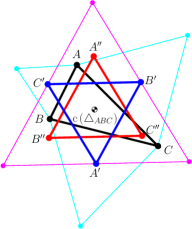
Figure 11: Outer Napoleon Triangles $\bigtriangleup_{A^{\prime}B^{\prime}C^{\prime}}$ and $\bigtriangleup_{A^{\prime\prime}B^{\prime\prime}C^{\prime\prime}}$ of $\bigtriangleup_{ABC}$ and $\bigtriangleup_{A^{\prime}B^{\prime}C^{\prime}}$, respectively, and $\bigtriangleup_{A^{\prime\prime}B^{\prime\prime}C^{\prime\prime}}$ is referred to as the double outer triangle of $\bigtriangleup_{ABC}$. Note that centroids of all triangles coincides, i.e. $\mathrm{c}\left(\bigtriangleup_{ABC}\right)=\mathrm{c}\left(\bigtriangleup_{A^{\prime}B^{\prime}C^{\prime}}\right)=\mathrm{c}\left(\bigtriangleup_{A^{\prime\prime}B^{\prime\prime}C^{\prime\prime}}\right)$.

The NNI-triplet $\left\{A,B,C\right\}$ defines an associated triangle with distinct vertices for each configuration, $\bigtriangleup_{A,B,C}:\mathfrak{S}\!\left(\sigma\right)\rightarrow\mathtt{Conf}\!\left(\mathbb{R}^{d},\left[3\right],\mathrm{\mathbf{0}}\right)$,

$$\bigtriangleup_{A,B,C}\left(\mathrm{\mathbf{x}}\right)\>{\mathbf{:}\!=}\>{\left[\begin{array}[]{@{}c@{}@{}c@{}@{}c@{}}\mathrm{c}\left(\mathrm{\mathbf{x}}|A\right),&\mathrm{c}\left(\mathrm{\mathbf{x}}|B\right),&\mathrm{c}\left(\mathrm{\mathbf{x}}|C\right)\end{array}\right]}^{\mathrm{T}}.$$ (33)

The double outer Napolean tranformation of $\bigtriangleup_{A,B,C}\left(\mathrm{\mathbf{x}}\right)$ returns symmetric target locations for $\mathrm{c}\left(\mathrm{\mathbf{x}}|A\right)$, $\mathrm{c}\left(\mathrm{\mathbf{x}}|B\right)$ and $\mathrm{c}\left(\mathrm{\mathbf{x}}|C\right)$, and the corresponding displacement of $\mathrm{c}\left(\mathrm{\mathbf{x}}|P\right)$, denoted $\mathtt{Noff}_{A,B,C}:\mathtt{Conf}\!\left(\mathbb{R}^{d}\!,J,\mathbf{r}\right)\rightarrow\mathbb{R}^{d}$, is given by the formula

$$\mathtt{Noff}_{A,B,C}\left(\mathrm{\mathbf{x}}\right)\>{\mathbf{:}\!=}\>\mathrm{c}\left(\mathrm{\mathbf{x}}|P\right)-\Gamma\cdot\mathtt{NT}\circ\bigtriangleup_{A,B,C}\left(\mathrm{\mathbf{x}}\right),$$ (34)

where $\Gamma:=\frac{1}{\left|P\right|}\left[\begin{array}[]{@{}c@{}@{}c@{}@{}c@{}}\left|A\right|,&\left|B\right|,&\left|C\right|\end{array}\right]\otimes\mathrm{\mathbf{I}}_{d}\in\mathbb{R}^{d\times 3d}$, and the vertices of the associated equilateral triangle with compensated offset of $\mathrm{c}\left(\mathrm{\mathbf{x}}|P\right)$ are

$${\left[\begin{array}[]{@{}c@{}@{}c@{}@{}c@{}}c_{A},&c_{B},&c_{C}\end{array}\right]}^{\mathrm{T}}\!\>{\mathbf{:}\!=}\>\mathtt{NT}\!\circ\!\bigtriangleup_{A,B,C}\left(\mathrm{\mathbf{x}}\right)\!+\!\mathrm{\mathbf{1}}_{3}\!\otimes\!\mathtt{Noff}_{A,B,C}\left(\mathrm{\mathbf{x}}\right)\!.\!\!$$ (36)

V-D2 Portal Maps

We now define a portal map, ${\mathtt{Port}}:\mathfrak{S}\!\left(\sigma\right)\rightarrow\mathtt{Portal}\left(\sigma,\tau\right)$, to be

$${\mathtt{Port}}\left(\mathrm{\mathbf{x}}\right)\!\!\>{\mathbf{:}\!=}\>\!\!\left\{\begin{array}[]{@{}l@{}@{}l@{}}\mathrm{\mathbf{x}}&\text{, if }\mathrm{\mathbf{x}}\!\in\!\mathtt{Portal}\left(\sigma,\tau\right)\!,\\ \left({\mathtt{Mrg}}\!\circ\!{\mathtt{Scl}}\!\circ\!{\mathtt{Ctr}}\right)\left(\mathrm{\mathbf{x}}\right)&\text{, otherwise,}\end{array}\right.\!\!\!$$ (39)

where ${\mathtt{Ctr}}:\mathfrak{S}\!\left(\sigma\right)\rightarrow\mathtt{Sym}\left(\sigma,\tau\right)$ rigidly translates the partial configurations, $\mathrm{\mathbf{x}}|A$, $\mathrm{\mathbf{x}}|B$ and $\mathrm{\mathbf{x}}|C$, to the new centroid locations, $c_{A}$, $c_{B}$ and $c_{C}$ (36), respectively, yielding a symmetric configuration,

$${\mathtt{Ctr}}\left(\mathrm{\mathbf{x}}\right)\!\>{\mathbf{:}\!=}\>\!\left\{\begin{array}[]{@{}l@{}@{}l@{}}\mathrm{x}_{i}&\text{, if }i\!\not\in\!P,\\ \mathrm{x}_{i}\!-\!\mathrm{c}\left(\mathrm{\mathbf{x}}|Q\right)\!+\!\mathrm{c}_{Q}&\text{, if }i\in Q,Q\in\left\{A,B,C\right\}\!,\end{array}\right.\!\!\!\!\!$$ (42)

It is important to observe that ${\mathtt{Ctr}}$ keeps the barycenter of $\mathrm{\mathbf{x}}|P$ fixed, and so separating hyperplanes of the rest of clusters ascending and disjoint with $P$ are kept unchanged.

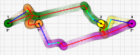
(a) (b)

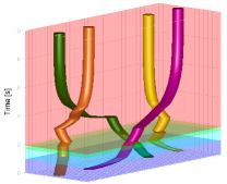
(c)

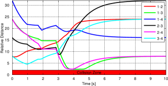
(d)

Figure 12: An illustrative navigation trajectory of the hybrid dynamics generated by the HNC algorithm for 4 disks in a planar ambient space. Disks are placed on the horizontal axis for both the initial and desired configurations in different orders, from left to right $\left(1,2,3,4\right)$ and $\left(3^{*},1^{*},4^{*},2^{*}\right)$ at the start and goal, respectively. (a) The sequence of trees associated with deployed local controllers during the execution of the hybrid navigation controller. (b) Centroidal trajectory of each disk colored according the active local controller, where $\mathrm{\mathbf{x}}_{c}\in\mathfrak{S}\!\left(\tau_{1}\right)\cap\mathfrak{S}\!\left(\tau_{2}\right)$, $\mathrm{\mathbf{x}}_{g}\in\mathfrak{S}\!\left(\tau_{2}\right)\cap\mathfrak{S}\!\left(\tau_{3}\right)$ and $\mathrm{\mathbf{x}}_{r}\in\mathfrak{S}\!\left(\tau_{3}\right)\cap\mathfrak{S}\!\left(\tau_{4}\right)$ shown by cyan, green and red dots, respectively, are portal configurations. (c) Space-time curve of disks (d) Pairwise distances between disks.

After obtaining a symmetric configuration in $\mathtt{Sym}\left(\sigma,\tau\right)$, ${\mathtt{Scl}}:\mathtt{Sym}\left(\sigma,\tau\right)\rightarrow\mathtt{Sym}\left(\sigma,\tau\right)$ rigidly translates each partial configuration, $\mathrm{\mathbf{x}}|A$, $\mathrm{\mathbf{x}}|B$ and $\mathrm{\mathbf{x}}|C$, to scale and fit into the corresponding consensus ball so that the new configuration simultaneously support both subtrees of $\sigma$ and $\tau$ rooted at $P$,

$${\mathtt{Scl}}\left(\mathrm{\mathbf{x}}\right) \!\>{\mathbf{:}\!=}\>\!\!\left\{\begin{array}[]{@{}l@{}l}\mathrm{x}_{i},&\text{, if }i\not\in P\\ \mathrm{x}_{i}\!+\!\zeta\!\cdot\left(\big{.}\mathrm{c}\left(\mathrm{\mathbf{x}}|Q\right)\!-\!\mathrm{c}\left(\mathrm{\mathbf{x}}|P\right)\!\right)&\text{, if }\begin{array}[]{@{}c@{}}i\!\in\!Q,\\ \!Q\!\in\!\left\{A,B,C\right\}\!,\end{array}\end{array}\right.\!\!\!\!\!\!\!\!$$ (47)

where $\zeta\in[0,\infty)$ is a scale parameter defined as

$$\zeta\>{\mathbf{:}\!=}\>\max_{Q\in\left\{A,B,C\right\}}\max\left(\frac{r\left(\mathrm{\mathbf{x}}|Q\right)+\alpha}{r_{Q}\left(\mathrm{\mathbf{x}}\right)},1\right)-1.$$ (48)

Here, $\alpha>0$ is a safety margin as used in (22), and $r\left(\mathrm{\mathbf{x}}|Q\right)$ (12) denotes the centroidal radius of partial configuration $\mathrm{\mathbf{x}}|Q$ and $r_{Q}\left(\mathrm{\mathbf{x}}\right)$ (31) is the radius of its consensus ball. Note that ${\mathtt{Scl}}$ preserves the symmetry of the configurations, i.e. centroids $\mathrm{c}\left(\mathrm{\mathbf{x}}|A\right)$, $\mathrm{c}\left(\mathrm{\mathbf{x}}|B\right)$ and $\mathrm{c}\left(\mathrm{\mathbf{x}}|C\right)$ still form an equilateral triangle after the mapping, and lefts the barycenter of $\mathrm{\mathbf{x}}|P$ unchanged.

Finally, ${\mathtt{Mrg}}:\mathtt{Sym}\left(\sigma,\tau\right)\rightarrow\mathtt{Sym}\left(\sigma,\tau\right)$ iteratively translates and merges partial configurations of common complementary clusters of $\sigma$ and $\tau$, in a bottom-up fashion starting at $P$, to simultaneously support both hierarchies $\sigma$ and $\tau$,

$${\mathtt{Mrg}}\left(\mathrm{\mathbf{x}}\right)\>{\mathbf{:}\!=}\>{\mathtt{Mrg}}_{P}\left(\mathrm{\mathbf{x}}\right),$$ (49)

where for any $I\in\left\{P\right\}\cup\mathrm{Anc}\left(P,\sigma\right)$

$${\mathtt{Mrg}}_{I}\left(\mathrm{\mathbf{x}}\right)\!\>{\mathbf{:}\!=}\>\!\left\{\begin{array}[]{@{}l@{}l}\mathrm{\mathbf{x}}&\text{, if }I=J,\\ ({\mathtt{Mrg}}_{\mathrm{Pr}\left(I,\tau\right)}\circ{\mathtt{Sep}}_{I})\left(\mathrm{\mathbf{x}}\right)&\text{, otherwise.}\end{array}\right.$$ (52)

Here, ${\mathtt{Sep}}_{I}$ separates complementary clusters $I$ and ${I}^{-\sigma}$ such that the clearance between every agent in $I\cup{I}^{-\sigma}$ and the associated separating hyperplane is at least $\alpha$ units (i.e. if $\hat{\mathrm{\mathbf{x}}}={\mathtt{Sep}}_{I}\left(\mathrm{\mathbf{x}}\right)$ for some $\mathrm{\mathbf{x}}\in\left(\mathbb{R}^{d}\right)^{J}$ with $\mathrm{s}_{I,\sigma}\left(\mathrm{\mathbf{x}}\right)\neq 0$, then $\eta_{k,K,\sigma}\left(\hat{\mathrm{\mathbf{x}}}\right)\geq r_{k}+\alpha$ for any $k\in K$, $K\in\left\{I,{I}^{-\sigma}\right\}$): for any $j\in J$

$${\mathtt{Sep}}_{I}\left(\mathrm{\mathbf{x}}\right)_{\!j}\!\>{\mathbf{:}\!=}\>\!\!\left\{\begin{array}[]{@{}l@{}l}\mathrm{\mathbf{x}}_{j}&\text{, if }j\!\not\in\!\mathrm{Pr}\left(I,\sigma\right)\!,\\ \mathrm{\mathbf{x}}_{j}\!+\!2\lambda\frac{|{K}^{-\sigma}|}{\left|\mathrm{Pr}\left(K,\sigma\right)\right|}\!\frac{\mathrm{s}_{K,\sigma}\left(\mathrm{\mathbf{x}}\right)}{\left\|\mathrm{s}_{K,\sigma}\left(\mathrm{\mathbf{x}}\right)\right\|}&\text{, if }\begin{array}[]{@{}c@{}}j\in K,\\ \!K\!\in\!\!\left\{\!I,{I}^{-\sigma}\!\right\}\!,\end{array}\end{array}\right.\!\!\!\!\!\!\!\!$$ (57)

where the required amount of centroidal separation, $\lambda\in[0,\infty)$, is given by

$$\lambda\>{\mathbf{:}\!=}\>\!\!\max_{\begin{subarray}{c}k\in K\\ K\in\left\{I,{I}^{-\sigma}\right\}\end{subarray}}\!\!\max\left(\big{.}\!-\left(\eta_{k,K,\sigma}\left(\mathrm{\mathbf{x}}\right)\!-\!r_{k}\!-\!\alpha\right),0\right).$$ (58)

Note that since $\mathrm{c}\left(\mathrm{\mathbf{x}}|P\right)=\mathrm{c}\left(\hat{\mathrm{\mathbf{x}}}|P\right)$ for any $\mathrm{\mathbf{x}}\in\mathfrak{S}\!\left(\sigma\right)$ and $\hat{\mathrm{\mathbf{x}}}=\left({\mathtt{Scl}}\circ{\mathtt{Ctr}}\right)\left(\mathrm{\mathbf{x}}\right)$, we always have $\mathrm{s}_{I,\sigma}\left(\hat{\mathrm{\mathbf{x}}}\right)\neq 0$ for any $I\in\left\{P\right\}\cup\mathrm{Anc}\left(P,\sigma\right)$, which is required for ${\mathtt{Sep}}_{I}$ to be well defined. Further, using (57), one can verify that $\mathrm{c}\left(\mathrm{\mathbf{x}}|\mathrm{Pr}\left(I,\sigma\right)\right)=\mathrm{c}\left(\hat{\mathrm{\mathbf{x}}}|\mathrm{Pr}\left(I,\sigma\right)\right)=\mathrm{c}\left(\tilde{\mathrm{\mathbf{x}}}|\mathrm{Pr}\left(I,\sigma\right)\right)$ for $\tilde{\mathrm{\mathbf{x}}}={\mathtt{Sep}}_{I}\left(\hat{\mathrm{\mathbf{x}}}\right)$, and so $\mathrm{s}_{A,\sigma}\left(\tilde{\mathrm{\mathbf{x}}}\right)\neq 0$ for any $A\in\mathrm{Anc}\left(I,\sigma\right)$, which guarantees that recursive calls of ${\mathtt{Sep}}_{I}$ in the computation of ${\mathtt{Port}}$ are always well-defined.

We find it useful to summarize some critical properties of the portal map for the strata of $\mathtt{HC}_{\text{2-means}}$ as:

Theorem 6

The NNI-graph $\mathcal{N}_{J}=\left(\mathcal{BT}_{J},\mathcal{E}_{\mathcal{N}}\right)$ is a subgraph of the $\mathtt{HC}_{\text{2-means}}$ adjacency graph $\mathcal{A}_{J}=\left(\mathcal{BT}_{J},\mathcal{E}_{\mathcal{A}}\right)$, i.e. for any pair $\left(\sigma,\tau\right)$ of NNI-adjacent trees in $\mathcal{BT}_{J}$, $\mathtt{Portal}\left(\sigma,\tau\right)\neq\emptyset$. Further, given an edge, $\left(\sigma,\tau\right)\in\mathcal{E}_{\mathcal{N}}\subset\mathcal{E}_{\mathcal{A}}$, a geometric realization via the map ${\mathtt{Port}}_{\left(\sigma,\tau\right)}:\mathfrak{S}\!\left(\sigma\right)\rightarrow\mathtt{Portal}\left(\sigma,\tau\right)$ (39) can be computed in quadratic, $\mathrm{O}\left(\left|J\right|^{2}\right)$, time with the number of leaves, $\left|J\right|$.

• See Appendix B-A. ∎

VI Numerical Simulations

For the sake of clarity, we first illustrate the behavior of the hybrid system defined in Section V for the case of four disks moving in a two-dimensional ambient space.

In order to visualize in this simple setting the most complicated instance of collision-free navigation and observe maximal number of transitions between local controllers, we pick the initial, $\mathrm{\mathbf{x}}\in\mathfrak{S}\!\left(\tau_{1}\right)$, and desired configurations, $\mathrm{\mathbf{x}}^{*}\in\mathfrak{S}\!\left(\tau_{4}\right)$, where disks are placed on the horizontal axis and left-to-right ordering of their labels are $\left(1,2,3,4\right)$ and $\left(3^{*},1^{*},4^{*},2^{*}\right)$, respectively, and their corresponding clustering trees are $\tau_{1}\in\mathcal{BT}_{\left[4\right]}$ and $\tau_{4}\in\mathcal{BT}_{\left[4\right]}$, see Fig. 12.

The resultant trajectory of each disk following the hybrid navigation planner in Section V, the relative distance between each pair of disks and the sequence of trees associated with visited hierarchical strata are shown in Fig. 12. Here, the disks start following the local controller associated with $\tau_{1}$ until they enter in finite time the domain of the following local controller associated with $\tau_{2}$ at $\mathrm{\mathbf{x}}_{c}\in\mathfrak{S}\!\left(\tau_{1}\right)\cap\mathfrak{S}\!\left(\tau_{2}\right)$ — shown by cyan dots in Fig. 12. After a finite time navigating in $\mathfrak{S}\!\left(\tau_{2}\right)$ and $\mathfrak{S}\!\left(\tau_{3}\right)$, respectively, the group enters the domain of the goal controller $f_{\tau_{4},\mathrm{\mathbf{x}}^{*}}$ (Table IV) at $\mathrm{\mathbf{x}}_{r}\in\mathfrak{S}\!\left(\tau_{3}\right)\cap\mathfrak{S}\!\left(\tau_{4}\right)$ — shown by red dots in Fig. 12, and $f_{\tau_{4},\mathrm{\mathbf{x}}^{*}}$ asymptotically steers the disks to the desired configuration $\mathrm{\mathbf{x}}^{*}\in\mathfrak{S}\!\left(\tau_{4}\right)$. Finally, note that the total number of binary trees over four leaves is 15; however, our hybrid navigation planner reactively deploys only 4 of them.

We now consider a similar, but slightly more complicated setting: a group of six disks in a plane where agents are initially placed evenly on the horizontal axes and switch their positions at the destination as shown in Fig. 13(a), which is also used in [17] as an example of complicated multi-agent arrangements. While steering the disks towards the goal, the hybrid navigation planner automatically deploys only 6 local controllers out of the family of 945 local controllers. The time evolution of the disk is illustrated in Fig. 13(a).

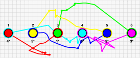
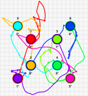
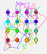
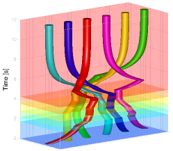
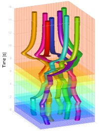
(a)	(b)	(c)

Figure 13: Example trajectories of the hybrid vector field planner for (a) 6, (b) 8 and (c) 16 disks in a planar ambient space. (top) Trajectory and (bottom) state-time curve of each disk. Each colored time interval demonstrates the execution duration of an activated local controller. Dots correspond to the portal configurations where transitions between local controllers occur at.

Finally, to demonstrate the efficiency of the deployment policy of our hybrid planner, we separately consider groups of 8 and 16 disks in an ambient plane, illustrated in Fig. 13. The eight disks are initially located at the corner of two squares whose centroids coincide and the perimeter of one is twice of the perimeter of the other. At the destination, disks switch their locations as illustrated in Fig. 13(b). For sixteen disk case, disks are initially placed at the vertices of a 4 by 4 grid, and their task is to switch their location as illustrated in Fig. 13(c). Although there are a large number of local controllers for the case of groups of 8 and 16 disks ($\left|\mathcal{BT}_{\left[8\right]}\right|>10^{5}$ and $\left|\mathcal{BT}_{\left[16\right]}\right|>6\times 10^{15}$), our hybrid navigation planner only deploys 9 and 19 local controllers, respectively.

The number of potentially available local controllers for a group of $n$ disks (28) grows super exponentially with $n$. On the other hand, if agents have perfect sensing and actuation modelled as in the present paper, the hybrid navigation planner automatically deploys at most $\frac{1}{2}\left(n-1\right)\left(n-2\right)$ local controllers [85], illustrating the computational efficiency of our construction.

VII Conclusion

In this paper, we introduce a novel application of clustering to the problem of coordinated robot navigation. The notion of hierarchical clustering offers a natural abstraction for ensemble task encoding and control in terms of precise yet flexible organizational specifications at different resolutions. Based on this new abstraction, we propose a provably correct generic hierarchical navigation framework for collision-free motion design towards any given destination via a sequence of hierarchy preserving controllers. For the 2-means divisive hierarchical clustering [69], based on a topological characterization of the underlying space, we present a centralized online (completely reactive) and computationally efficient instance of our hierarchical navigation framework for disk-shaped robots, which generalizes to an arbitrary number of disks and ambient space dimension.

Specifically, matching the component problem statements of Section IV to their subsequent resolution: we address Problem 1 in Theorem 4 (guaranteeing that the construction of Table IV results in a hierarchy invariant vector field planner); we address Problem 2 in Theorem 5 (guaranteeing that the construction of Table V results in a reactive strategy that finds, given any non-goal tree, an edge in the graph of all hierarchies leading to a new tree that is closer to the desired goal hierarchy); and we address Problem 3 in Theorem 6 (providing a geometric realization in the configuration space of the combinatorial edge toward the physical goal). The efficacy of this overarching strategy is guaranteed by Theorem 1 (proving the correctness of these problems steps and their resolutions as presented in Table III).

Work now in progress targets more practical settings in the field of robotics including navigating around obstacles in compact spaces and a distributed implementation of our navigation framework. We are also exploring a number of application settings for hierarchical formation specification and control including problems of perception, perceptual servoing, anomaly detection and automated exploration and various problems of multi-agent coordination.

In the longer term, especially when the scalability and efficiency of hierarchical protocols in sensor networks for information routing and aggregation is of concern [88], these methods suggest a promising unifying framework to simultaneously handle control, communication and information aggregation (fusion) in multi-agent systems.

Appendix A Properties of The Hierarchy Invariant Vector Field

Although the recursive definition of the hierarchy preserving navigation policy, $f_{\tau,\mathrm{\mathbf{y}}}$, in Table IV expresses an efficient encoding of intra-cluster and inter-cluster interactions and dependencies of individuals, which we suspect will prove to have value for distributed settings, it yields a discontinuous vector field complicating the qualitative (existence, uniqueness, invariance and stability) analysis, as anticipated from the proof structure of Theorem 4 in Table VI. We find it convenient to proceed instead by developing an alternative, equivalent representation of this vector field. Namely, we introduce a family of continuous and piecewise smooth covering vector fields whose application over a partition (derived from their covering domains) of the stratum yields a continuous piecewise smooth flow (identical to that generated by the original construction) which is considerably easier to analyze because it admits an interpretation as a sequential composition [10] over the covering family.

We find it useful to first observe that the original construction yields a well defined and effectively computable function.

Proposition 3

The recursion in Table IV results in a well defined function, $f_{\tau,\mathrm{\mathbf{y}}}:\mathfrak{S}\!\left(\tau\right)\rightarrow\left(\mathbb{R}^{d}\right)^{J}$, that can be computed for each configuration $\mathrm{\mathbf{x}}\in\mathfrak{S}\!\left(\tau\right)$ in $\mathrm{O}\left(\left|J\right|^{2}\right)$ time.

• See Appendix B-B. ∎

TABLE VI: The Proof Structure of Theorem 4 : Logical Dependencies

• Proposition 3 (Quadratic Time Function) [A, p.3 $\Leftarrow$ B-B, p.B-B] • Proposition 4 (Continuous ​&​ Piecewise Smooth) [A-A, p.4 $\Leftarrow$ B-C,p.B-C] – Lemma 5 (Child Partition Block) [A-F, p.5] • Proposition 5 (Domain Covering Induced Partition) ​[A-A, ​p.5 ​$\Leftarrow$​ B-D, ​p.B-D] • Proposition 6 (Equivalent Vector Field) [A-A, p.6 $\Leftarrow$ B-E, p.B-E] • Proposition 13 (Stratum Positive Invariance) [A-D, p.13] – Recalls Proposition 5, Proposition 6 – Proposition 9 (Substratum Positive Invariance) [A-C, p.9 $\Leftarrow$ B-I, p.B-I] * Lemma 7 (Invariance - Base Case 1) [B-I, p.7 $\Leftarrow$ B-M, p.B-M] * Lemma 8 (Invariance - Base Case 2) [B-I, p.8 $\Leftarrow$ B-N, p.B-N] * Lemma 9 (Invariance - Recursion) [B-I, p.9 $\Leftarrow$ B-O, p.B-O] • Proposition 14 (Stratum Existence & Uniqueness) [A-D, p.14] – Recalls Proposition 5, Proposition 6 – Proposition 10 (Substratum ​Existence ​Uniqueness) ​[A-C, ​p.10 ​$\Leftarrow$​ B-H, ​p.B-H] * Recalls Proposition 4, Proposition 9. * Lemma 3 (Relative Centroidal Dynamics) [A-F, p.3 $\Leftarrow$ B-K,p.B-K] * Lemma 4 (Configuration Bound Radius) [A-F, p.4 $\Leftarrow$ B-L, p.B-L] · Recalls Lemma 3. – Proposition 15 (Stratum Stability) [A-D, p.15] * Recalls Proposition 6, Proposition 9. * Proposition 8 (Substratum Policy Selection) [A-C, p.8 $\Leftarrow$ B-G, p.B-G] · Recalls Proposition 5. · Lemma 6 (Partition Refinement) [A-F, p.6] * Proposition 11 (Finite Time Prepares Relation) [A-C, p.11 $\Leftarrow$ B-J, p.B-J] · Lemma 10 (Case (i) in Definition 5) [B-J, p.10 $\Leftarrow$ B-P, p.B-P] · Lemma 11 (Case (ii) in Definition 5) [B-J, p.11 $\Leftarrow$ B-Q, p.B-Q] · Lemma 12 (Case (iii) in Definition 5) [B-J, p.12 $\Leftarrow$ B-R, p.B-R] • Proposition 7 (Substratum Prepares Graph) [A-B, p.11 $\Leftarrow$ B-F, p.B-F] – Recalls Lemma 5. • Proposition 12 (Nondegenerate Execution) [A-C, p.12] – Recalls Proposition 8, Proposition 9. – Lemma 2 (Closed Substratum Domain) [A-C, p.2]

A-A An Equivalent System Model

Key for understanding the hierarchy preserving navigation policy, $f_{\tau,\mathrm{\mathbf{y}}}$, in Table IV is the observation that for any configuration $\mathrm{\mathbf{x}}\in\mathfrak{S}\!\left(\tau\right)$ the list of visited clusters of $\tau$ satisfying base conditions during the recursive computation of $f_{\tau,\mathrm{\mathbf{y}}}$ defines a partition $\mathcal{J}$ of $J$ compatible with $\tau$, i.e. $\mathcal{J}\subset\mathcal{C}\left(\tau\right)$.

TABLE VII: Local Control Policies in a Hierarchical Stratum

Let $\mathcal{J}$ be a partition of $J$ with $\mathcal{J}\subset\mathcal{C}\left(\tau\right)$, and $\mathrm{\mathbf{b}}=\left(\mathrm{b}_{I}\right)_{I\in\mathcal{J}}\in\left\{-1,+1\right\}^{\mathcal{J}}$. For any desired $\mathrm{\mathbf{y}}\in\mathfrak{S}\!\left(\tau\right)$, supporting $\tau\in\mathcal{BT}_{J}$, and any initial $\mathrm{\mathbf{x}}\in\mathcal{D}\left(\mathcal{J},\mathrm{\mathbf{b}}\right)$ (63), the local control policy, $h_{\mathcal{J},\mathrm{\mathbf{b}}}:\mathcal{D}\left(\mathcal{J},\mathrm{\mathbf{b}}\right)\rightarrow\left(\mathbb{R}^{d}\right)^{J}$, $\displaystyle h_{\mathcal{J},\mathrm{\mathbf{b}}}\left(\mathrm{\mathbf{x}}\right)\>{\mathbf{:}\!=}\>\hat{h}_{\mathcal{J},\mathrm{\mathbf{b}}}\left(\mathrm{\mathbf{x}},\mathrm{\mathbf{0}},J\right),$ is recursively computed using the post-order traversal of $\tau$ starting at the root cluster $J$ with the zero control input $\mathrm{\mathbf{0}}\in\left(\mathbb{R}^{d}\right)^{J}$ as follows: for any $\mathrm{\mathbf{u}}\in\left(\mathbb{R}^{d}\right)^{J}$ and $I\in\mathcal{V}_{\tau}\left(\mathcal{J}\right)$ (67), $\rotatebox{90.0}{Base Cases}\left\{\begin{array}[]{c}\\[1.42262pt] \\[1.42262pt] \\[1.42262pt] \\[1.42262pt] \\[1.42262pt] \\[1.42262pt] \end{array}\right.$ $\rotatebox{90.0}{Recursion}\left\{\begin{array}[]{c}\\[1.70717pt] \\[1.70717pt] \\[1.70717pt] \\[1.70717pt] \\[1.70717pt] \\[1.70717pt] \end{array}\right.$ 1. function $\hat{\mathrm{\mathbf{u}}}=\hat{h}_{\mathcal{J},\mathrm{\mathbf{b}}}\left(\mathrm{\mathbf{x}},\mathrm{\mathbf{u}},I\right)$ 2. if $I\in\mathcal{J}$, 3. if $\mathrm{b}_{I}=+1$ 4. $\hat{\mathrm{\mathbf{u}}}\leftarrow f_{A}\left(\mathrm{\mathbf{x}},\mathrm{\mathbf{u}},I\right)$ (16), 5. else 6. $\hat{\mathrm{\mathbf{u}}}\leftarrow f_{S}\left(\mathrm{\mathbf{x}},\mathrm{\mathbf{u}},I\right)$ (26), 7. end 8. else 9. $\left\{I_{L},I_{R}\right\}\leftarrow\mathrm{Ch}\left(I,\tau\right)$, 10. $\hat{\mathrm{\mathbf{u}}}_{L}\leftarrow\hat{h}_{\mathcal{J},\mathrm{\mathbf{b}}}\left(\mathrm{\mathbf{x}},\mathrm{\mathbf{u}},I_{L}\right)$, 11. $\hat{\mathrm{\mathbf{u}}}_{R}\leftarrow\hat{h}_{\mathcal{J},\mathrm{\mathbf{b}}}\left(\mathrm{\mathbf{x}},\hat{\mathrm{\mathbf{u}}}_{L},I_{R}\right)$, 12. $\hat{\mathrm{\mathbf{u}}}\leftarrow f_{H}\left(\mathrm{\mathbf{x}},\hat{\mathrm{\mathbf{u}}}_{R},I\right)$ (21), 13. end 14. return $\hat{\mathrm{\mathbf{u}}}$ % Attracting Field % Split Separation Field % Recursion for Left Child % Recursion for Right Child % Split Preserving Field

Now observe, depending on which base condition holds (Table IV.2) or Table IV.4)), every block $I$ of partition $\mathcal{J}$, associated with any fixed configuration $\mathrm{\mathbf{x}}\in\mathcal{D}_{A}\left(I\right)\cup\,\left(\mathfrak{S}\!\left(\tau\right)\setminus\mathcal{D}_{H}\left(I\right)\right)$, can be associated with a binary scalar $\hat{\mathrm{b}}_{I}\left(\mathrm{\mathbf{x}}\right)\in\left\{-1,+1\right\}$ such that

$$\hat{\mathrm{b}}_{I}\left(\mathrm{\mathbf{x}}\right)=\left\{\begin{array}[]{ll}+1&\text{, if }\mathrm{\mathbf{x}}\in\mathcal{D}_{A}\left(I\right),\\ -1&\text{, if }\mathrm{\mathbf{x}}\not\in\mathcal{D}_{A}\left(I\right)\cup\mathcal{D}_{H}\left(I\right),\end{array}\right.$$ (61)

where $\mathcal{D}_{A}\left(I\right)$ and $\mathcal{D}_{H}\left(I\right)$ are defined as in (V-B) and (20), respectively. We will use this configuration space labeling scheme to recast the hierarchy preserving control policy $f_{\tau,\mathrm{\mathbf{y}}}$ as an online sequential composition of a family of continuous and piecewise smooth local controllers indexed by partitions of $J$ compatible with $\tau$ and associated binary vectors as follows.

A partition $\mathcal{J}$ of $J$ is said to be compatible with $\tau\in\mathcal{BT}_{J}$ if and only if $\mathcal{J}\subset\mathcal{C}\left(\tau\right)$, and denote by $\mathcal{P}_{J}\left(\tau\right)$ the set of partitions of $J$ compatible with $\tau$. Accordingly, define $\mathcal{SP}_{J}\left(\tau\right)$ to be the set of substratum policy indices,

$$\mathcal{SP}_{J}\left(\tau\right)\>{\mathbf{:}\!=}\>\left\{\left(\mathcal{J},\mathrm{\mathbf{b}}\right)\Big{|}\,\mathcal{J}\in\mathcal{P}_{J}\left(\tau\right),\mathrm{\mathbf{b}}\in\left\{-1,+1\right\}^{\mathcal{J}}\right\}.$$ (62)

For any partition $\mathcal{J}\in\mathcal{P}_{J}\left(\tau\right)$ of $J$ and $\mathrm{\mathbf{b}}\>{\mathbf{:}\!=}\>\left(\mathrm{b}_{I}\right)_{I\in\mathcal{J}}\in\left\{-1,+1\right\}^{\mathcal{J}}$, the domain $\mathcal{D}\left(\mathcal{J},\mathrm{\mathbf{b}}\right)$ of a local control policy $h_{\mathcal{J},\mathrm{\mathbf{b}}}$, presented in Table VII, is defined to be

$$\mathcal{D}\left(\mathcal{J},\mathrm{\mathbf{b}}\right)\>{\mathbf{:}\!=}\>\bigcap_{I\in\mathcal{J}}\left(\Big{.}\right.\!\!\mathcal{D}_{B}\left(I,\mathrm{b}_{I}\right)\,{$\cap$}\!\!\bigcap_{K\in\mathrm{Anc}\;\left(I,\tau\right)}\!\!\!\!\mathcal{D}_{H}\left(K\right)\!\!\left.\Big{.}\right)\!,$$ (63)

where the set of configurations satisfying the base condition associated with cluster $I$ of $\mathcal{J}$ and binary scalar $\mathrm{b}_{I}$ is given by

$$\mathcal{D}_{B}\left(I,\mathrm{b}_{I}\right)\>{\mathbf{:}\!=}\>\left\{\begin{array}[]{@{}c@{}@{}l}\mathcal{D}_{A}\left(I\right)&\text{, if }\mathrm{b}_{I}=+1,\\ \mathfrak{S}\!\left(\tau\right)&\text{, if }\mathrm{b}_{I}=-1,\end{array}\right.$$ (66)

and all ancestors $K\in\mathrm{Anc}\left(I,\tau\right)$ of $I$ in $\tau$ satisfy the recursion condition of having properly separated children clusters described by $\mathcal{D}_{H}\left(K\right)$ (20). Accordingly, let $\mathcal{V}_{\tau}\left(\mathcal{J}\right)$ denote the set of clusters of $\tau$ visited during the recursive computation of $h_{\mathcal{J},\mathrm{\mathbf{b}}}$ in Table VII,

$$\mathcal{V}_{\tau}\left(\mathcal{J}\right)\>{\mathbf{:}\!=}\>\left\{K\in\mathcal{C}\left(\tau\right)\big{|}K\supseteq I,I\in\mathcal{J}\right\}.$$ (67)

Note that $J\in\mathcal{V}_{\tau}\left(\mathcal{J}\right)$ since $\mathcal{J}$ is a partition of the root cluster $J$ and any block $I\in\mathcal{J}$ satisfies $I\subseteq J$.

Observe that each local control policy $h_{\mathcal{J},\mathrm{\mathbf{b}}}$ is a recursive composition of continuous functions of $\mathrm{\mathbf{x}}$, so it is continuous:

Proposition 4

The recursion in Table VII results in a continuous and piecewise smooth function, $h_{\mathcal{J},\mathrm{\mathbf{b}}}:\mathfrak{S}\!\left(\tau\right)\rightarrow\left(\mathbb{R}^{d}\right)^{J}$.

• See Appendix B-C. ∎

To conclude our introduction of the family of covering fields in Table VII, we now observe that the vector field $f_{\tau,\mathrm{\mathbf{y}}}$ in Table IV is an online concatenation of continuous local controllers, $h_{\mathcal{J},\mathrm{\mathbf{b}}}$, of Table VII using a policy selection method described in Table VIII, summarized as:

TABLE VIII: Policy Selection Algorithm

For any initial $\mathrm{\mathbf{x}}\in\mathfrak{S}\!\left(\tau\right)$ and desired $\mathrm{\mathbf{y}}\in\mathfrak{S}\!\left(\tau\right)$, supporting $\tau\in\mathcal{BT}_{J}$, the policy selection algorithm, $p:\mathfrak{S}\!\left(\tau\right)\rightarrow\mathcal{SP}_{J}\left(\tau\right)$, $\displaystyle p\left(\mathrm{\mathbf{x}}\right)\>{\mathbf{:}\!=}\>\hat{p}\left(\mathrm{\mathbf{x}},J\right),$ recursively generates a local policy index in $\mathcal{SP}_{J}\left(\tau\right)$ (62) using the post-order traversal of $\tau$ starting at the root cluster $J$ as follows: for any $I\in\mathcal{C}\left(\tau\right)$, $\rotatebox{90.0}{Base Cases}\left\{\begin{array}[]{c}\\[1.70717pt] \\[1.70717pt] \\[1.70717pt] \\[1.70717pt] \\[1.70717pt] \\[1.70717pt] \end{array}\right.$ $\rotatebox{90.0}{Recursion}\left\{\begin{array}[]{c}\\[1.42262pt] \\[1.42262pt] \\[1.42262pt] \\[1.42262pt] \\[1.42262pt] \\[1.42262pt] \\[1.42262pt] \end{array}\right.$ 1. function $(\hat{\mathcal{I}},\hat{\mathrm{\mathbf{b}}})=\hat{p}\left(\mathrm{\mathbf{x}},I\right)$ 2. if $\mathrm{\mathbf{x}}\in\mathcal{D}_{A}\left(I\right)$ (V-B), 3. $\hat{\mathcal{I}}\leftarrow\left\{I\right\}$, 4. $\hat{\mathrm{\mathbf{b}}}\leftarrow+1$, 5. else if $\mathrm{\mathbf{x}}\not\in\mathcal{D}_{H}\left(I\right)$ (20), 6. $\hat{\mathcal{I}}\leftarrow\left\{I\right\}$, 7. $\hat{\mathrm{\mathbf{b}}}\leftarrow-1$, 8. else 9. $\left\{I_{L},I_{R}\right\}\leftarrow\mathrm{Ch}\left(I,\tau\right)$, 10. $(\hat{\mathcal{I}}_{L},\hat{\mathrm{\mathbf{b}}}_{L})\leftarrow\hat{p}\left(\mathrm{\mathbf{x}},I_{L}\right)$, 11. $(\hat{\mathcal{I}}_{R},\hat{\mathrm{\mathbf{b}}}_{R})\leftarrow\hat{p}\left(\mathrm{\mathbf{x}},I_{R}\right)$, 12. $\hat{\mathcal{I}}\leftarrow\hat{\mathcal{I}}_{L}\cup\hat{\mathcal{I}}_{R}$, 13. $\hat{\mathrm{\mathbf{b}}}\leftarrow\hat{\mathrm{\mathbf{b}}}_{L}\|\hat{\mathrm{\mathbf{b}}}_{R}$, 14. end 15. return $(\hat{\mathcal{I}},\hat{\mathrm{\mathbf{b}}})$

Proposition 5

For any given configuration $\mathrm{\mathbf{x}}\in\mathfrak{S}\!\left(\tau\right)$ the policy selection algorithm $p$ in Table VIII always returns a valid policy index, $\left(\mathcal{J,\mathrm{\mathbf{b}}}\right)=p\left(\mathrm{\mathbf{x}}\right)$, in $\mathcal{SP}_{J}\left(\tau\right)$ (62) such that the domain $\mathcal{D}\left(\mathcal{J},\mathrm{\mathbf{b}}\right)$ (63) of the associated local control policy $h_{\mathcal{J},\mathrm{\mathbf{b}}}$ (Table VII) contains $\mathrm{\mathbf{x}}$, i.e.

$$\mathrm{\mathbf{x}}\in\left(\mathcal{D}\circ p\right)\left(\mathrm{\mathbf{x}}\right).$$ (68)

• See Appendix B-D.∎

Proposition 6

For any given configuration $\mathrm{\mathbf{x}}\in\mathfrak{S}\!\left(\tau\right)$, the vector field $f_{\tau,\mathrm{\mathbf{x}}}$ (Table IV) and the local control policy $h_{\mathcal{J},\mathrm{\mathbf{b}}}\left(\mathrm{\mathbf{x}}\right)$ (Table VII) selected as $\left(\mathcal{J,\mathrm{\mathbf{b}}}\right)=p\left(\mathrm{\mathbf{x}}\right)$ (Table VIII) generate the same control (velocity) inputs, i.e.

$$f_{\tau,\mathrm{\mathbf{y}}}\left(\mathrm{\mathbf{x}}\right)=h_{p\left(\mathrm{\mathbf{x}}\right)}\left(\mathrm{\mathbf{x}}\right).$$ (69)

• See Appendix B-E. ∎

Since the hierarchy invariant field $f_{\tau,\mathrm{\mathbf{y}}}$ is defined for entire $\mathfrak{S}\!\left(\tau\right)$, it is useful to remark that the domains, $\mathcal{D}\left(\mathcal{J},\mathrm{\mathbf{b}}\right)$ (63), of local control policies, $h_{\mathcal{J},\mathrm{\mathbf{b}}}$, define a cover of $\mathfrak{S}\!\left(\tau\right)$ indexed by partitions of $J$ compatible with $\tau$ and associated binary vectors.

A-B Online Sequential Composition of Substratum Policies

We now briefly describe the logic behind online sequential composition [10] of substratum policies.

To characterize our policy selection strategy, we first define a priority measure for each local controller $h_{\mathcal{J},\mathrm{\mathbf{b}}}$ associated with a partition $\mathcal{J}\in\mathcal{P}_{J}\left(\tau\right)$ of $J$ and a binary vector $\mathrm{\mathbf{b}}\in\left\{-1,+1\right\}^{\mathcal{J}}$ to be

$$\mathtt{priority}\left(\mathcal{J},\mathrm{\mathbf{b}}\right)\>{\mathbf{:}\!=}\>\sum_{I\in\mathcal{J}}\mathrm{b}_{I}\left|I\right|^{2}.$$ (70)

Note that the maximum and minimum of the priority measure is attained at the coarsest partition $\left\{J\right\}$ of $J$, and $\mathrm{b}_{J}=+1$ and $\mathrm{b}_{J}=-1$, respectively,

$$\mathtt{priority}\left(\left\{J\right\},+1\right) =\left|J\right|^{2},$$ (71a)

$$\mathtt{priority}\left(\left\{J\right\},-1\right) =-\left|J\right|^{2}.$$ (71b)

Accordingly, we shall refer to the local control policy with index $\left(\left\{J\right\},+1\right)$ as the goal policy since it has the highest priority and asymptotically steers all configurations in its domain $\mathcal{D}\left(\left\{J\right\},+1\right)$(63) to $\mathrm{\mathbf{y}}$ following the negated gradient of $V\left(\mathrm{\mathbf{x}}\right)=\frac{1}{2}\left\|\mathrm{\mathbf{x}}-\mathrm{\mathbf{y}}\right\|$, i.e. for any $\mathrm{\mathbf{x}}\in\mathcal{D}\left(\left\{J\right\},+1\right)$

$$h_{\left\{J\right\},+1}\left(\mathrm{\mathbf{x}}\right)=-\nabla V\left(\mathrm{\mathbf{x}}\right)=-(\mathrm{\mathbf{x}}-\mathrm{\mathbf{y}}).$$ (72)

Note that since the root cluster $J$ has no ancestor, i.e. $\mathrm{Anc}\left(J,\tau\right)=\emptyset$, by definition (63), $\mathcal{D}\left(\left\{J\right\},+1\right)=\mathcal{D}_{A}\left(J\right)$, and $\mathcal{D}_{A}\left(J\right)$ (V-B) contains the goal configuration $\mathrm{\mathbf{y}}$.

We now introduce an abstract connection between local policies for high-level planning:

Definition 4

Let $\left(\mathcal{J},\mathrm{\mathbf{b}}\right),(\mathcal{J}^{\prime},\mathrm{\mathbf{b}}^{\prime})\in\mathcal{SP}_{J}\left(\tau\right)$ be two distinct substratum policy indices. Then $h_{\mathcal{J},\mathrm{\mathbf{b}}}$ is said to prepare $h_{\mathcal{J}^{\prime},\mathrm{\mathbf{b}}^{\prime}}$ if and only if all trajectories of $h_{\mathcal{J},\mathrm{\mathbf{b}}}$ starting in its domain $\mathcal{D}\left(\mathcal{J},\mathrm{\mathbf{b}}\right)$, possibly excluding a set of measure zero, reach $\mathcal{D}(\mathcal{J}^{\prime},\mathrm{\mathbf{b}}^{\prime})$ in finite time.

Accordingly, define the prepares graph $\mathcal{PG}=\left(\mathcal{SP}_{J}\left(\tau\right),\mathcal{E}_{\mathcal{PG}}\right)$ to have vertex set $\mathcal{SP}_{J}\left(\tau\right)$(62) with a policy index $\left(\mathcal{J},\mathrm{\mathbf{b}}\right)\!\in\!\mathcal{SP}_{J}\left(\tau\right)$ connected to another policy index $(\mathcal{J}^{\prime},\mathrm{\mathbf{b}}^{\prime})$ by a directed edge in $\mathcal{E}_{\mathcal{PG}}$ if and only if $h_{\mathcal{J},\mathrm{\mathbf{b}}}$ prepares $h_{\mathcal{J}^{\prime},\mathrm{\mathbf{b}}^{\prime}}$.

Although, the prepares graph $\mathcal{PG}$ is the most critical component of the sequential composition framework [10] defining a discrete abstraction of continuous control policies, the exponentially growing cardinality of substratum policies, discussed in Appendix A-E, and the lack of an explicit characterization of globally asymptotically stable configurations of substratum policies make it usually difficult to compute the complete prepares graph.

Alternatively, we introduce a computationally efficient and recursively constructed graph of substratum policies that is nicely compatible with our needs, yielding a subgraph of the prepares graph, where every policy index is connected to the goal policy index $\left(\left\{J\right\},+1\right)$ through a directed path, as follows.

Definition 5

Let $\widehat{\mathcal{PG}}=(\mathcal{SP}_{J}\left(\tau\right),\widehat{\mathcal{E}}_{\mathcal{PG}})$ be a graph with vertex list $\mathcal{SP}_{J}\left(\tau\right)$, and a policy index $\left(\mathcal{J},\mathrm{\mathbf{b}}\right)\in\mathcal{SP}_{J}\left(\tau\right)$ that is connected to another policy index $(\mathcal{J}^{\prime},\mathrm{\mathbf{b}}^{\prime})\in\mathcal{SP}_{J}\left(\tau\right)$ by a directed edge in $\widehat{\mathcal{E}}_{\mathcal{PG}}$ if and only if at least one of the following properties holds:

1. (Complement) There exists a singleton cluster $I\in\mathcal{J}$ such that $\mathrm{b}_{I}=-1$, and $\mathcal{J}^{\prime}=\mathcal{J}$ and $\mathrm{\mathbf{b}}^{\prime}\in\left\{-1,+1\right\}^{\mathcal{J}^{\prime}}$ with $\mathrm{b}^{\prime}_{I}=+1$ and $\mathrm{b}^{\prime}_{D}=\mathrm{b}_{D}$ for all $D\in\mathcal{J}\setminus\left\{I\right\}$.

2. (Split) There exists a nonsingleton cluster $I\in\mathcal{J}$ such that $\mathrm{b}_{I}=-1$, and $\mathcal{J}^{\prime}=\mathcal{J}\setminus\left\{I\right\}\cup\mathrm{Ch}\left(I,\tau\right)$ and $\mathrm{\mathbf{b}}^{\prime}\in\left\{-1,+1\right\}^{\mathcal{J}^{\prime}}$ with $\mathrm{b}^{\prime}_{K}=-1$ for all $K\in\mathrm{Ch}\left(I,\tau\right)$ and $\mathrm{b}^{\prime}_{D}=\mathrm{b}_{D}$ for all $D\in\mathcal{J}\setminus\mathrm{Ch}\left(I,\tau\right)$.

3. (Merge) There exists a nonsingleton cluster $I\!\in\!\mathcal{C}\left(\tau\right)$ such that $\mathrm{Ch}\left(I,\tau\right)\!\subset\!\mathcal{J}$ and $\mathrm{b}_{K}\!=\!+1$ for all $K\!\in\!\mathrm{Ch}\left(I,\tau\right)$, and $\mathcal{J}^{\prime}=\mathcal{J}\setminus\mathrm{Ch}\left(I,\tau\right)\cup\left\{I\right\}$ and $\mathrm{\mathbf{b}}^{\prime}\in\left\{-1,+1\right\}^{\mathcal{J}^{\prime}}$ with $\mathrm{b}^{\prime}_{I}=+1$ and $\mathrm{b}^{\prime}_{D}=\mathrm{b}_{D}$ for all $D\in\mathcal{J}\setminus\mathrm{Ch}\left(I,\tau\right)$.

Note that, since $\mathcal{J}$ is compatible with $\tau$, i.e. $\mathcal{J}\subset\mathcal{C}\left(\tau\right)$, if $\left|\mathcal{J}\right|>1$, then there exists a cluster $I\in\mathcal{C}\left(\tau\right)$ such that $\mathrm{Ch}\left(I,\tau\right)\subset\mathcal{J}$ (Lemma 5). Hence, for any policy index $\left(\mathcal{J},\mathrm{\mathbf{b}}\right)\neq\left(\left\{J\right\},+1\right)$ there always exists a policy index $(\mathcal{J}^{\prime},\mathrm{\mathbf{b}}^{\prime})\neq\left(\mathcal{J},\mathrm{\mathbf{b}}\right)$ satisfying one of these conditions, (i)-(iii) above. Thus, the out-degree of a policy index $\left(\mathcal{J},\mathrm{\mathbf{b}}\right)\neq\left(\left\{J\right\},+1\right)$ in $\widehat{\mathcal{PG}}$ is at least one, whereas the goal policy index $\left(\left\{J\right\},+1\right)$ in $\widehat{\mathcal{PG}}$ has an out-degree of zero. We summarize some important properties of $\widehat{\mathcal{PG}}$ as follows:

Proposition 7

The graph $\widehat{\mathcal{PG}}=(\mathcal{SP}_{J}\left(\tau\right),\widehat{\mathcal{E}}_{\mathcal{PG}})$, as defined in Definition 5, is an acyclic subgraph of the prepares graph $\mathcal{PG}=(\mathcal{SP}_{J}\left(\tau\right),\mathcal{E}_{\mathcal{PG}})$ (Definition 4) such that all policy indices in $\mathcal{SP}_{J}\left(\tau\right)$ are connected to the goal policy index $\left(\left\{J\right\},+1\right)$ through directed paths in $\widehat{\mathcal{E}}_{\mathcal{PG}}$, of length at most $\mathrm{O}\left(\left|J\right|^{2}\right)$ hops, along which $\mathtt{priority}$ (70) is strictly increasing, i.e. for any $\left(\big{.}\right.\!\left(\mathcal{J},\mathrm{\mathbf{b}}\right)\!,(\mathcal{J}^{\prime},\mathrm{\mathbf{b}}^{\prime})\!\!\left.\big{.}\right)\in\widehat{\mathcal{E}}_{\mathcal{PG}}$

$$\mathtt{priority}(\mathcal{J}^{\prime},\mathrm{\mathbf{b}}^{\prime})>\mathtt{priority}\left(\mathcal{J},\mathrm{\mathbf{b}}\right).$$ (73)

• See Appendix B-F. ∎

Although a given local policy can prepare more than one potential successor (i.e. higher priority), our policy selection method chooses the one with the strictly highest priority:

Proposition 8

For any given $\mathrm{\mathbf{x}}\in\mathfrak{S}\!\left(\tau\right)$ the policy selection method, $p$, in Table VIII always returns the index of a local controller with the maximum priority among all local controllers whose domain contains $\mathrm{\mathbf{x}}$,

$$p\left(\mathrm{\mathbf{x}}\right)=\operatornamewithlimits{arg\ max}_{\begin{subarray}{c}(\mathcal{J}^{\prime},\mathrm{\mathbf{b}}^{\prime})\in\mathcal{SP}_{J}\left(\tau\right)\\ \mathrm{\mathbf{x}}\in\mathcal{D}\left(\mathcal{J}^{\prime},\mathrm{\mathbf{b}}^{\prime}\right)\end{subarray}}\mathtt{priority}(\mathcal{J}^{\prime},\mathrm{\mathbf{b}}^{\prime}).$$ (74)

and all the other available local controllers have strictly lower priorities.

• See Appendix B-G. ∎

A-C Qualitative Properties of Substratum Policies

We now list important qualitative (existence, uniqueness, invariance and stability) properties of the substratum control policies of Table VII. Let $\mathcal{J}$ be a partition of $J$ compatible with $\tau$, i.e. $\mathcal{J}\subset\mathcal{C}\left(\tau\right)$, and $\mathrm{\mathbf{b}}$ is a binary vector in $\left\{-1,1\right\}^{\mathcal{J}}$.

Proposition 9

The domain, $\mathcal{D}\left(\mathcal{J},\mathrm{\mathbf{b}}\right)$ (63), of a substratum policy, $h_{\mathcal{J},\mathrm{\mathbf{b}}}$ (Table VII), is positive invariant.

• See Appendix B-I. ∎

Proposition 10

(Substratum Existence and Uniqueness) The vector field $h_{\mathcal{J},\mathrm{\mathbf{b}}}$ (Table VII) is locally Lipschitz in $\mathfrak{S}\!\left(\tau\right)$; and for any initial $\mathrm{\mathbf{x}}\in\mathcal{D}\left(\mathcal{J},\mathrm{\mathbf{b}}\right)\subset\mathfrak{S}\!\left(\tau\right)$ there always exists a compact (bounded and closed) subset $W$ of $\mathcal{D}\left(\mathcal{J},\mathrm{\mathbf{b}}\right)$ (63) such that all trajectories of $h_{\mathcal{J},\mathrm{\mathbf{b}}}$ starting at $\mathrm{\mathbf{x}}$ remain in $W$ for all future time.

Therefore, there is a unique continuous and piecewise smooth flow of $h_{\mathcal{J},\mathrm{\mathbf{b}}}$ in $\mathcal{D}\left(\mathcal{J},\mathrm{\mathbf{b}}\right)$ that is defined for all future time.

• See Appendix B-H. ∎

Proposition 11

(Finite Time Prepares Relation) Each local control policy, $h_{\mathcal{J},\mathrm{\mathbf{b}}}$, with the exception of the goal controller $h_{\left\{J\right\},+1}$, steers (almost) all configurations in its domain, $\mathcal{D}\left(\mathcal{J},\mathrm{\mathbf{b}}\right)$, to the domain, $\mathcal{D}\left(\mathcal{J}^{\prime},\mathrm{\mathbf{b}}^{\prime}\right)$, of another local controller, $h_{\mathcal{J}^{\prime},\mathrm{\mathbf{b}}^{\prime}}$, at a higher $\,\mathtt{priority}$ (70) in finite time.

• See Appendix B-J. ∎

Proposition 12

(Nonzero Execution Time) Let $\mathrm{\mathbf{x}}^{t}$ be a trajectory of the local control policy $h_{\mathcal{J},\mathrm{\mathbf{b}}}$ starting at $\mathrm{\mathbf{x}}^{0}\in\mathcal{D}\left(\mathcal{J},\mathrm{\mathbf{b}}\right)$ such that $p\left(\mathrm{\mathbf{x}}^{0}\right)=\left(\mathcal{J},\mathrm{\mathbf{b}}\right)$.

Then the local controller is guaranteed to steers the group for a nonzero time until reaching the domain of a local controller at a higher $\mathtt{priority}$ (70), i.e.

$$\inf_{t}\left\{t\geq 0\big{|}p\left(\mathrm{\mathbf{x}}^{t}\right)\neq\left(\mathcal{J},\mathrm{\mathbf{b}}\right)\right\}>0.$$ (75)

Recall that for any configuration $\mathrm{\mathbf{x}}\in\mathfrak{S}\!\left(\tau\right)$ the policy selection method in Table VIII always yields the index of the local controller with the highest priority among all local controllers whose domains contain $\mathrm{\mathbf{x}}$ (Proposition 8). Hence, since the initial configuration $\mathrm{\mathbf{x}}^{0}$ is not included in the domain of any other local controller with a higher priority than $\mathtt{priority}(\mathcal{J},\mathrm{\mathbf{b}})$ and domains of local controllers are closed relative to $\mathfrak{S}\!\left(\tau\right)$ (Lemma 2), there always exists an open set around $\mathrm{\mathbf{x}}^{0}$ which does not intersect with the domain of any local controller at a higher priority than $\mathtt{priority}(\mathcal{J},\mathrm{\mathbf{b}})$. Thus, since its domain is positively invariant (Proposition 9), $h_{\mathcal{J},\mathrm{\mathbf{b}}}$ is guaranteed to steer the configuration in the intersection of this open set and $\mathcal{D}\left(\mathcal{J},\mathrm{\mathbf{b}}\right)$ for a nonzero time. ∎

A-D Qualitative Properties of Stratum Policies

We now proceed with some important qualitative (existence, uniqueness, invariance and stability) properties of the hierarchy preserving navigation policy of Table IV.

Proposition 13

The stratum $\mathfrak{S}\!\left(\tau\right)$ is positive invariant under the hierarchy-invariant control policy, $f_{\tau,\mathrm{\mathbf{y}}}$ (Table IV).

• Recall that the domains, $\mathcal{D}$ (63), of local control policies in Table VII define a cover of $\mathfrak{S}\!\left(\tau\right)$ (Proposition 5) each of whose elements is positively invariant under the flow of the associated local policy (Proposition 9). Thus, the result follows since the hierarchy preserving vector field $f_{\tau,\mathrm{\mathbf{y}}}$ is equivalent to online sequential composition of local control policies of Table VII based on the policy selection algorithm in Table VIII (Proposition 6). ∎

Proposition 14

(Stratum Existence and Uniqueness) The hierarchy invariance control policy, $f_{\tau,\mathrm{\mathbf{y}}}$ (Table IV), has a unique, continuous and piecewise smooth flow, $\varphi^{t}$, in $\mathfrak{S}\!\left(\tau\right)$, defined for all $t\geq 0$.

• Recall from Proposition 6 that $f_{\tau,\mathrm{\mathbf{y}}}$ is equivalent to online sequential composition of a family of substratum policies which have unique, continuous and piecewise smooth flows, defined for all $t\geq 0$, in their positive invariant domains (Proposition 10). Since their domains define a finite closed cover of $\mathfrak{S}\!\left(\tau\right)$ (Proposition 5), the unique, continuous and piecewise flow of $f_{\tau,\mathrm{\mathbf{y}}}$ is constructed by piecing together trajectories of these substratum policies. ∎

Proposition 15

Any $\mathrm{\mathbf{y}}\in\mathfrak{S}\!\left(\tau\right)$ is an asymptotically stable equilibrium point of the hierarchy-invariant control policy, $f_{\tau,\mathrm{\mathbf{y}}}$ (Table IV), whose basin of attraction includes $\mathfrak{S}\!\left(\tau\right)$, except a set of measure zero.

• Using the equivalence (Proposition 6) of the hierarchy preserving field $f_{\tau,\mathrm{\mathbf{y}}}$ and the sequential composition of substratum control policies of Table VII based on the policy selection method in Table VIII, the result can be obtained as follows.

  Since $\mathtt{priority}$ (70) is an integer-valued function with bounded range (71), using Proposition 8 and Proposition 11, one can conclude that the disks starting at almost any configuration in $\mathfrak{S}\!\left(\tau\right)$ reach the domain $\mathcal{D}\left(\left\{J\right\},+1\right)$ of the goal policy $h_{\left\{J,+1\right\}}$ in finite time after visiting at most $\mathrm{O}\left(\left|J\right|^{2}\right)$ of other local control policies. Note that $\mathrm{\mathbf{y}}\in\mathcal{D}\left(\left\{J\right\},+1\right)$. Then, the goal policy $h_{\left\{J\right\},+1}$

  $$h_{\left\{J\right\},+1}\left(\mathrm{\mathbf{x}}\right)=-\nabla{$\frac{1}{2}$}\left\|\mathrm{\mathbf{x}}-\mathrm{\mathbf{y}}\right\|_{2}^{2}=-\left(\mathrm{\mathbf{x}}-\mathrm{\mathbf{y}}\right),$$ (76)

  asymptotically steers all configuration in $\mathcal{D}\left(\left\{J\right\},+1\right)$ to $\mathrm{\mathbf{y}}$ while keeping its domain of attraction $\mathcal{D}_{A}\left(J\right)$ positively invariant (Proposition 9), which completes the proof ∎

A-E On the Cardinality of Substratum Policies

To gain an appreciation for the computational efficiency of hierarchy preserving vector field in Table IV, we find it useful to have a brief discussion without proofs on the cardinality of the family of local control policies of Table VII. The number of partitions $\mathcal{P}_{J}\left(\tau\right)$ of $J$ compatible with a cluster hierarchy $\tau\in\mathcal{BT}_{J}$ is recursively given by

$$\left|\mathcal{P}_{J}\left(\tau\right)\right|=1+\left|\mathcal{P}_{J}\left(\tau_{L}\right)\right|\left|\mathcal{P}_{J}\left(\tau_{R}\right)\right|,$$ (78)

where $\tau_{L},\tau_{R}$ denote the left and right subtrees of $\tau$, respectively. For any caterpillar tree $\sigma\in\mathcal{BT}_{J}$, $\left|\mathcal{P}_{J}\left(\sigma\right)\right|=\left|J\right|$ since one of two subtrees of $\sigma$ is always one-leaf tree. On the other hand, for a balanced tree $\gamma\in\mathcal{BT}_{J}$ the cardinality of partitions of $J$ compatible with $\gamma$ grows exponentially,

$$\sqrt{2}^{\left|J\right|}\leq\left|\mathcal{P}_{J}\left(\gamma\right)\right|\leq\frac{4}{5}\sqrt{\frac{5}{2}}^{\left|J\right|},$$ (79)

for $\left|J\right|=2^{k}$, $k\in\mathbb{N}_{+}=\left\{1,2,3,\ldots\right\}$; for example, $\left|\mathcal{P}_{\left[2\right]}\left(\gamma\right)\right|=2$, $\left|\mathcal{P}_{\left[4\right]}\left(\gamma\right)\right|=5$, $\left|\mathcal{P}_{\left[8\right]}\left(\gamma\right)\right|=26$ and $\left|\mathcal{P}_{\left[16\right]}\left(\gamma\right)\right|=677$. In addition to a partition $\mathcal{J}$ of $J$ compatible with $\tau$, every local control policy $h_{\mathcal{J},\mathrm{\mathbf{b}}}$ is indexed by a binary variable of size $\left|\mathcal{J}\right|$ with a possible choice of $2^{\left|\mathcal{J}\right|}$ values. Therefore, the number of local control policies $h_{\mathcal{J},\mathrm{\mathbf{b}}}$ grows exponentially with the group size, $\left|J\right|$.

A-F A Set of Useful Observations on Substratum Policies

Here we introduce a set of useful lemmas that constitute building blocks for proving some qualitative properties of substratum policies presented in Appendix A-C. Let $\mathcal{J}$ be a partition of $J$ compatible with $\tau$, i.e. $\mathcal{J}\subset\mathcal{C}\left(\tau\right)$, and $\mathrm{\mathbf{b}}$ is a binary vector in $\left\{-1,+1\right\}^{\mathcal{J}}$.

Lemma 2

The domain, $\mathcal{D}\left(\mathcal{J},\mathrm{\mathbf{b}}\right)$ (63), of each substratum policy, $h_{\mathcal{J},\mathrm{\mathbf{b}}}$, is closed relative to $\mathfrak{S}\!\left(\tau\right)$.

• Using the continuity of functions in the predicates used to define them, one can conclude that for any $I\in\mathcal{C}\left(\tau\right)$ sets $\mathcal{D}_{A}\left(I\right)$ (V-B) and $\mathcal{D}_{H}\left(I\right)$ (20) are closed relative to $\mathfrak{S}\!\left(\tau\right)$. Hence, since the intersection of arbitrary many closed sets are closed [91], the domain $\mathcal{D}\left(\mathcal{J},\mathrm{\mathbf{b}}\right)$ (63) of each local controller $h_{\mathcal{J},\mathrm{\mathbf{b}}}$ is closed relative to $\mathfrak{S}\!\left(\tau\right)$. ∎

A critical observation used for bounding the centroidal configuration radius (Lemma 4) and the range of a trajectory of a substratum policy (Proposition 10) is:

Lemma 3

(Relative Centroidal Dynamics) Let $\mathrm{\mathbf{x}}\in\mathfrak{S}\!\left(\tau\right)$ and

$$\mathrm{\mathbf{u}}=h_{\mathcal{J},\mathrm{\mathbf{b}}}\left(\mathrm{\mathbf{x}}\right).$$ (84)

Then, the centroidal dynamics of any cluster $I\in\mathcal{V}_{\tau}\left(\mathcal{J}\right)$ (67) visited during recursive computation of $h_{\mathcal{J},\mathrm{\mathbf{b}}}$ (Table VII), except the root $J$, satisfies

$$\mathrm{c}\left(\mathrm{\mathbf{u}}|I\right) =-\mathrm{c}\left(\mathrm{\mathbf{x}}\!-\!\mathrm{\mathbf{y}}|I\right)+2\alpha_{P}\left(\mathrm{\mathbf{x}},\mathrm{\mathbf{v}}_{P}\right)\!\frac{\left|{I}^{-\tau}\right|}{\left|P\right|}\frac{\mathrm{s}_{I\!}\left(\mathrm{\mathbf{x}}\right)}{\left\|\mathrm{s}_{I\!}\left(\mathrm{\mathbf{x}}\right)\right\|}$$

$$\hskip 85.35826pt+\mathrm{c}\left(\mathrm{\mathbf{u}}|P\right)+\mathrm{c}\left(\mathrm{\mathbf{x}}\!-\!\mathrm{\mathbf{y}}|P\right),$$ (85)

for some $\mathrm{\mathbf{v}}_{P}\in\left(\mathbb{R}^{d}\right)^{J}$ associated with parent cluster $P=\mathrm{Pr}\left(I,\tau\right)$; whereas we have for the root cluster $J$

$$\mathrm{c}\left(\mathrm{\mathbf{u}}|J\right)=-\mathrm{c}\left(\mathrm{\mathbf{x}}-\mathrm{\mathbf{y}}|J\right).$$ (86)

• See Appendix B-K. ∎

Lemma 4

(Upper Bound on Configuration Radius) Let $\mathrm{\mathbf{x}}^{t}$ denote a trajectory of $h_{\mathcal{J},\mathrm{\mathbf{b}}}$ (Table VII) starting at any initial $\mathrm{\mathbf{x}}^{0}\in\mathcal{D}\left(\mathcal{J},\mathrm{\mathbf{b}}\right)$ (63) for $t\geq 0$.

Then, the centroidal configuration radius, $r\left(\mathrm{\mathbf{x}}^{t}|J\right)$ (12), is bounded above for all $t\geq 0$ by a certain finite value, $R\left(\mathrm{\mathbf{x}}^{0},\mathrm{\mathbf{y}}\right)$, depending on $\mathrm{\mathbf{x}}^{0}$ and $\mathrm{\mathbf{y}}$, i.e.

$$r\left(\mathrm{\mathbf{x}}^{t}|J\right)\leq R\left(\mathrm{\mathbf{x}}^{0},\mathrm{\mathbf{y}}\right)<\infty,\quad\forall t\geq 0.$$ (87)

• See Appendix B-L. ∎

Lemma 5

If $\mathcal{J}$ is not the trivial partition, i.e. $\left|\mathcal{J}\right|>1$, then there always exists a cluster $I\in\mathcal{C}\left(\tau\right)$ such that $\mathrm{Ch}\left(I,\tau\right)\subset\mathcal{J}$.

• Define the depth of cluster $I\in\mathcal{C}\left(\tau\right)$ in $\tau$ to be the number of its ancestors, $\left|\mathrm{Anc}\left(I,\tau\right)\right|$.

  Let $K\in\mathcal{J}$ be a cluster in $\mathcal{J}$ with the maximal depth, i.e.

  $$\left|\mathrm{Anc}\left(K,\tau\right)\right|=\operatornamewithlimits{arg\ max}_{D\in\mathcal{J}}\left|\mathrm{Anc}\left(D,\tau\right)\right|.$$ (88)

  Then, we now show that ${K}^{-\tau}$ is also in $\mathcal{J}$, and so $I=\mathrm{Pr}\left(K,\tau\right)$ satisfies the lemma.

  Proof by a contradiction. Suppose that ${K}^{-\tau}$ is not in $\mathcal{J}$. Since $\mathcal{J}$ is a partition of $J$ compatible with $\tau$, then some descendant $D\in\mathrm{Des}\left({K}^{-\tau},\tau\right)$ is in $\mathcal{J}$. Note that $\left|\mathrm{Anc}\left(K,\tau\right)\right|=\left|\mathrm{Anc}\left({K}^{-\tau}\right)\right|<\left|\mathrm{Anc}\left(D,\tau\right)\right|$, which contradicts (88). ∎

Lemma 6

Let $\mathcal{J}$ and $\mathcal{J}^{\prime}$ be two distinct partitions of $J$ compatible with $\tau$, i.e. $\mathcal{J}\neq\mathcal{J}^{\prime}\subset\mathcal{C}\left(\tau\right)$. Then, at least one of the followings always holds

1. ($\mathcal{J}$ Partially Refines $\mathcal{J}^{\prime}$) There exists a cluster $K^{\prime}\in\mathcal{J}^{\prime}$ with a nontrivial partition $\mathcal{K}^{\prime}$ such that $\mathcal{K}^{\prime}\subset\mathcal{J}$.

2. ($\mathcal{J}^{\prime}$ Partially Refines $\mathcal{J}$) There exists a cluster $K\in\mathcal{J}$ with a nontrivial partition $\mathcal{K}$ such that $\mathcal{K}\subset\mathcal{J}^{\prime}$.

• For any $j\in J$, let $\mathcal{J}\left(j\right)$ denote the unique element of $\mathcal{J}$ containing $j$.

  Since $\mathcal{J}\neq\mathcal{J}^{\prime}$, let $K^{\prime}\in\mathcal{J}^{\prime}\setminus\mathcal{J}$ be an unshared cluster. Since both $\mathcal{J}$ and $\mathcal{J}^{\prime}$ are partitions of $J$ compatible with $\tau$, we have either $\mathcal{J}(k^{\prime})\subsetneq K^{\prime}$ or $\mathcal{J}(k^{\prime})\supsetneq K^{\prime}$ for all $k^{\prime}\in K^{\prime}$. If $\mathcal{J}(k^{\prime})\subsetneq K^{\prime}$ for all $k^{\prime}\in K^{\prime}$, then $\mathcal{K}^{\prime}=\left\{\mathcal{J}(k^{\prime})\big{|}k^{\prime}\in K^{\prime}\right\}$ defines a partition of $K^{\prime}$ and we obtain Lemma 6.(i). Otherwise, by symmetry, we have Lemma 6.(ii). Thus, the lemma follows. ∎

Appendix B Proofs

B-A Proof of Theorem 6

• To prove the first part of the result, we shall consider ${\mathtt{Port}}_{\sigma,\tau}$ as a mapping from $\mathfrak{S}\!\left(\sigma\right)$ to $\left(\mathbb{R}^{d}\right)^{J}$ and verify that ${\mathtt{Port}}_{\sigma,\tau}\left(\mathfrak{S}\!\left(\sigma\right)\right)\subseteq\mathtt{Portal}\left(\sigma,\tau\right)$.

By definition, the restriction of ${\mathtt{Port}}_{\sigma,\tau}$ to $\mathtt{Portal}\left(\sigma,\tau\right)$ is the identity map on $\mathtt{Portal}\left(\sigma,\tau\right)$. Hence, we only need to show that ${\mathtt{Port}}_{\sigma,\tau}\left(\mathfrak{S}\!\left(\sigma\right)\setminus\mathtt{Portal}\left(\sigma,\tau\right)\right)\subseteq\mathtt{Portal}\left(\sigma,\tau\right)$.

Let $\mathrm{\mathbf{y}}={\mathtt{Ctr}}\left(\mathrm{\mathbf{x}}\right)$ and $\mathrm{\mathbf{z}}={\mathtt{Scl}}\left(\mathrm{\mathbf{y}}\right)$ be intermediate configurations during the portal transformation of a configuration $\mathrm{\mathbf{x}}\in\mathfrak{S}\!\left(\sigma\right)\setminus\mathtt{Portal}\left(\sigma,\tau\right)$ into $\mathrm{\mathbf{w}}={\mathtt{Mrg}}\left(\mathrm{\mathbf{z}}\right)={\mathtt{Port}}\left(\mathrm{\mathbf{x}}\right)$.

First, recall that rigid transformations and scaling of partial configurations preserve their clustering structure [29]. Hence, the common subtrees of $\sigma$ and $\tau$ rooted at $A$, $B$ and $C$ are preserved after each transformation by ${\mathtt{Ctr}}$ (42), ${\mathtt{Scl}}$ (47) and ${\mathtt{Mrg}}$ (49).

Second, each partial configuration of the symmetric configuration $\mathrm{\mathbf{y}}\in\mathtt{Sym}\left(\sigma,\tau\right)$ associated with $\left(\sigma,\tau\right)$ is properly translated by ${\mathtt{Scl}}$ (47) so that each of them lies in the corresponding consensus ball, i.e. $r\left(\mathrm{\mathbf{z}}|Q\right)<r_{Q}\left(\mathrm{\mathbf{z}}\right)$ for all $Q\in\left(A,B,C\right)$. Hence, the partial configuration $\mathrm{\mathbf{z}}|P$ supports both of the subtrees of $\sigma$ and $\tau$ rooted at $P$.

Finally, if $P=J$, then the result simply follows since $\mathrm{\mathbf{z}}=\mathrm{\mathbf{w}}\in\mathtt{Portal}\left(\sigma,\tau\right)$. Otherwise, for every $I\in\left\{P\right\}\cup\mathrm{Anc}\left(P,\sigma\right)$, ${\mathtt{Mrg}}$ (49) iteratively separates the common complementary clusters $I$ and ${I}^{-\sigma}$ of $\sigma$ and $\tau$, in a bottom up fashion starting at cluster $P$, to support the subtrees of $\sigma$ and $\tau$ rooted at $\mathrm{Pr}\left(I,\sigma\right)$. Note that in the base case $\mathrm{\mathbf{z}}$ supports both of the subtrees of $\sigma$ and $\tau$ rooted at $P$ and ${P}^{-\sigma}$; and at the termination at cluster $J$, $\mathrm{\mathbf{w}}$ supports both trees $\sigma$ and $\tau$, i.e. $\mathrm{\mathbf{w}}\in\mathtt{Portal}\left(\sigma,\tau\right)$.

We now proceed with the computational properties of ${\mathtt{Port}}_{\sigma,\tau}$. As stated in the proof of Proposition 3, the inclusion test of a configuration for being in a hierarchical stratum can be computed in $\mathrm{O}\left(\left|J\right|^{2}\right)$ time, from which one conclude that the inclusion test for being in $\mathtt{Portal}\left(\sigma,\tau\right)$ can also be computed in $\mathrm{O}\left(\left|J\right|^{2}\right)$ time. If the given configuration is not a portal configuration, then the computation of ${\mathtt{Port}}_{\sigma,\tau}$(39) requires cluster centroids of $\sigma$, which can be computed in linear, $\mathrm{O}\left(\left|J\right|\right)$, time as described in the proof of Proposition 3. Given cluster centroids, one can compute ${\mathtt{Ctr}}$ (42) and ${\mathtt{Scl}}$ (47) in linear, $\mathrm{O}\left(\left|J\right|\right)$, time since the Napoleon transformation $\mathtt{NT}$ of an arbitrary triangle can be computed in constant, $\mathrm{O}\left(1\right)$, time [87]. Finally, given the cluster centroids, each iteration of ${\mathtt{Mrg}}$ (49) can be computed in linear $\mathrm{O}\left(\left|J\right|\right)$ time; and so all iterations of ${\mathtt{Mrg}}$ can be performed in $\mathrm{O}\left(\left|J\right|^{2}\right)$ time since it may require at most $\left|J\right|$ iterations. Thus, the result follows. ∎

B-B Proof of Proposition 3

• Recall from (V-B) that for any singleton cluster $I\in\mathcal{C}\left(\tau\right)$ we have $\mathcal{D}_{A}\left(I\right)=\mathfrak{S}\!\left(\tau\right)$. Hence, for any given $\mathrm{\mathbf{x}}\in\mathfrak{S}\!\left(\tau\right)$ the base condition $\mathrm{\mathbf{x}}\in\mathcal{D}_{A}\left(I\right)$ (Table IV.2) always holds at any singleton cluster $I\in\mathcal{C}\left(\tau\right)$. Moreover, the cardinality of any cluster passed as an argument in a recursive step of the evaluation must decrease relative to the calling cluster size (Table IV.7). Therefore, the recursion in Table IV terminates, in the worst case, after visiting all clusters of $\tau$ only once.

Since all vector fields ($f_{A}$ (16), $f_{H}$ (21) and $f_{S}$ (26)) used in Table IV are well defined over the entirety of their domain $\mathfrak{S}\!\left(\tau\right)$ with codomain $\left(\mathbb{R}^{d}\right)^{J}$, the recursion in Table IV results in a true function, $f_{\tau,\mathrm{\mathbf{y}}}:\mathfrak{S}\!\left(\tau\right)\rightarrow\left(\mathbb{R}^{d}\right)^{J}$, with well defined evaluation for each configuration $\mathrm{\mathbf{x}}\in\mathfrak{S}\!\left(\tau\right)$.

We now assess the computational complexity of the recursion in Table IV. Centroids of clusters of $\tau$ can be computed all at once in $\mathrm{O}\left(\left|J\right|\right)$ time using the post-order traversal of $\tau$ and the following recursive relation of cluster centroids: for any disjoint $A,B\subset J$,

$$\mathrm{c}\left(\mathrm{\mathbf{x}}|A\cup B\right)={$\frac{\left|A\right|}{\left|A\right|+\left|B\right|}$}\mathrm{c}\left(\mathrm{\mathbf{x}}|A\right)+{$\frac{\left|B\right|}{\left|A\right|+\left|B\right|}$}\mathrm{c}\left(\mathrm{\mathbf{x}}|B\right).$$ (89)

Given cluster centroids, $\eta_{i,I,\tau}\left(\mathrm{\mathbf{x}}\right)$ (7) can be computed in constant, $\mathrm{O}\left(1\right)$, time for any $i\in I$ and $I\in\mathcal{C}\left(\tau\right)$. Hence, since $\left|\mathcal{C}\left(\tau\right)\right|=2\left|J\right|-1$ for any $\tau\in\mathcal{BT}_{J}$ and $I=\left\{k\,\big{|}\,k\in K,K\in\mathrm{Ch}\left(I,\tau\right)\right\}$ for any nonsingleton cluster $I\in\mathcal{C}\left(\tau\right)$, we conclude:

• The inclusion test for being in $\mathfrak{S}\!\left(\tau\right)$ (6) can be computed in $\mathrm{O}\left(\left|J\right|^{2}\right)$.

• Given $\mathrm{\mathbf{x}}\in\mathfrak{S}\!\left(\tau\right)$, the inclusion test for being in $\mathcal{D}_{H}\left(I\right)$ (20) for any cluster $I\in\mathcal{C}\left(\tau\right)$ can be computed in $\mathrm{O}\left(\left|J\right|\right)$ time; and the recursion in Table IV requires such inclusion tests at most only once for all clusters of $\tau$ which can be computed in $\mathrm{O}\left(\left|J\right|^{2}\right)$ time.

• The vector fields $f_{A}$ (16), $f_{H}$ (21) and $f_{S}$ (26) at any cluster $I\in\mathcal{C}\left(\tau\right)$ can be computed in $\mathrm{O}\left(\left|J\right|\right)$ time; and, once again, the recursion in Table IV requires such computation at most at every cluster of $\tau$ all of which can be performed in $\mathrm{O}\left(\left|J\right|^{2}\right)$ time.

Finally, to conclude that $f_{\tau,\mathrm{\mathbf{y}}}$ is computable in $\mathrm{O}\left(\left|J\right|^{2}\right)$ time, we show that the inclusion test for being in $\mathcal{D}_{A}\left(I\right)$ (V-B) for all clusters $I\in\mathcal{C}\left(\tau\right)$ can be efficiently computed in $\mathrm{O}\left(\left|J\right|^{2}\right)$ time as follows. Given cluster centroids, $\mathcal{L}_{\overrightarrow{\mathrm{\mathbf{y}}}}{\left(\mathrm{x}_{k}\!-\!\mathrm{m}_{K\!}\left(\mathrm{\mathbf{x}}\right)\!\right)\!}^{\mathrm{T}}\mathrm{s}_{K\!}\left(\mathrm{\mathbf{x}}\right)$ (19) can be computed in constant, $\mathrm{O}\left(1\right)$, time for any $k\in K$, $K\in\mathcal{C}\left(\tau\right)$; and, likewise, $\mathcal{L}_{\overrightarrow{\mathrm{\mathbf{y}}}}\frac{1}{2}\left\|\mathrm{x}_{i}-\mathrm{x}_{j}\right\|^{2}$ (18) can be computed in constant $\mathrm{O}\left(1\right)$ time for any given pair $i\neq j\in J$. Further, using (V-B) and hierarchical relations of clusters, observe the following recursive relation of $\mathcal{D}_{A}\left(I\right)$: for any nonsingleton $I\in\mathcal{C}\left(\tau\right)$ and $\left\{I_{L},I_{R}\right\}=\mathrm{Ch}\left(I,\tau\right)$,

$$\mathcal{D}_{A}\left(I\right)=\mathcal{D}_{A}\left(I_{L}\right)\cap\mathcal{D}_{A}\left(I_{R}\right)\cap\widehat{\mathcal{D}}_{A}\left(I_{L},I_{R}\right),$$ (90)

subject to the base condition $\mathcal{D}_{A}\left(I\right)=\mathfrak{S}\!\left(\tau\right)$ for any singleton cluster $I\in\mathcal{C}\left(\tau\right)$, where

$$\widehat{\mathcal{D}}_{A}\left(I_{L},I_{R}\right)\!\!\>{\mathbf{:}\!=}\>\!\!\left\{\Big{.}\right.\!\!\mathrm{\mathbf{x}}\!\in\!\mathfrak{S}\!\left(\tau\right)\!\Big{|}\,\! \mathcal{L}_{\overrightarrow{\mathrm{\mathbf{y}}}}\!{$\frac{1}{2}$}\!\left\|\mathrm{x}_{i}\!-\!\mathrm{x}_{j}\right\|^{2}\!\geq\!\left(r_{i}\!+\!r_{j}\!\right)^{2}\!\!\!,\,\forall i\!\in\!\!I_{L},j\!\in\!\!I_{R},$$

$$\mathcal{L}_{\overrightarrow{\mathrm{\mathbf{y}}}}{\left(\mathrm{x}_{k}\!-\!\mathrm{m}_{K\!}\left(\mathrm{\mathbf{x}}\right)\!\right)\!}^{\mathrm{T}}\!\mathrm{s}_{K\!}\left(\mathrm{\mathbf{x}}\right)\!\geq\!0,\forall k\!\in\!K\!,K\!\in\!\left\{I_{L},I_{R}\right\}\!\!\!\left.\Big{.}\right\}\!.\!\!\!$$ (91)

Note that, given $\mathrm{\mathbf{x}}\in\mathfrak{S}\!\left(\tau\right)$, the inclusion test for being in $\widehat{\mathcal{D}}_{A}\left(I_{L},I_{R}\right)$ for the children $\left\{I_{L},I_{R}\right\}=\mathrm{Ch}\left(I,\tau\right)$ of any nonsingleton cluster $I\in\mathcal{C}\left(\tau\right)$ can be computed in $\mathrm{O}\left(\left|I_{L}\right|\left|I_{R}\right|+\left|I_{L}\right|+\left|I_{R}\right|\right)$ time.

Hence, given $\mathrm{\mathbf{x}}\in\mathfrak{S}\!\left(\tau\right)$, the inclusion test for being in $\mathcal{D}_{A}$ (V-B) for any cluster $I\in\mathcal{C}\left(\tau\right)$ and all its descendants in $\mathrm{Des}\left(I,\tau\right)$ can be computed at once in $\mathrm{O}\left(\left|I\right|^{2}\right)$ time using the post-order traversal of the subtree of $\tau$ rooted at $I$ and the recursive formulation (90) of $\mathcal{D}_{A}\left(I\right)$. This can be verified as follows. First, observe that the cluster set $\mathcal{C}\left(\tau\right)$ of $\tau$ can be recursively defined as:

$$\bullet \left\{j\right\}\in\mathcal{C}\left(\tau\right) j\in J$$ (Base Step) for all . (92a)

$$\bullet I,{I}^{-\tau}\!\in\!\mathcal{C}\left(\tau\right)\!\setminus\!\left\{J\right\} \mathrm{Pr}\left(I,\tau\right)\!\in\!\mathcal{C}\left(\tau\right)$$ (Recursion) If , then . (92b)

Accordingly, we provide a proof by structural induction [92]. For any $I\in\mathcal{C}\left(\tau\right)$:

• (Base Case) If $I$ is singleton, then the result simply holds since any singleton cluster $I\in\mathcal{C}\left(\tau\right)$ has no descendant in $\tau$ and satisfies $\mathcal{D}_{A}\left(I\right)=\mathfrak{S}\!\left(\tau\right)$.

• (Induction) Otherwise ($\left|I\right|\geq 2$), let $\left\{I_{L},I_{R}\right\}=\mathrm{Ch}\left(I,\tau\right)$. (Induction hypothesis) Suppose that the inclusion test for being in $\mathcal{D}_{A}$ for any child $K\in\mathrm{Ch}\left(I,\tau\right)$ and all its descendant in $\mathrm{Des}\left(K,\tau\right)$ is computable in $\mathrm{O}\left(\left|K\right|^{2}\right)$. Then, by the recursion in (90), the inclusion test for being in $\mathcal{D}_{A}$ for cluster $I$ and all its descendants in $\mathrm{Des}\left(I,\tau\right)$ only requires the extra test for being in $\widehat{\mathcal{D}}_{A}\left(I_{L},I_{R}\right)$ for the children $\left\{I_{L},I_{R}\right\}=\mathrm{Ch}\left(I,\tau\right)$ in addition to the inclusion test for every child $K\in\mathrm{Ch}\left(I,\tau\right)$ and its descendants in $\mathrm{Des}\left(K,\tau\right)$. Hence, the total computation cost for cluster $I$ and its descendants in $\tau$ is $\mathrm{O}\left(\left|I_{L}\right|^{2}\right)+\mathrm{O}\left(\left|I_{R}\right|^{2}\right)+\mathrm{O}\left(\Big{.}\left|I_{L}\right|\left|I_{R}\right|+\left|I_{R}\right|+\left|I_{R}\right|\right)=\mathrm{O}\left(\left|I\right|^{2}\right)$.

Therefore, since $\mathcal{C}\left(\tau\right)=\left\{J\right\}\cup\mathrm{Des}\left(J,\tau\right)$, given $\mathrm{\mathbf{x}}\in\mathfrak{S}\!\left(\tau\right)$ the inclusion test for being in $\mathcal{D}_{A}\left(I\right)$ for all clusters $I\in\mathcal{C}\left(\tau\right)$ can be computed at once in $\mathrm{O}\left(\left|J\right|^{2}\right)$ time, and this completes the proof. ∎

B-C Proof of Proposition 4

• To demonstrate how the recursion in Table VII recursively composes continuous vector fields, we shall recast $f_{A}$ (16), $f_{H}$ (21), $f_{S}$ (26) and the recursion $\hat{h}_{\mathcal{J},\mathrm{\mathbf{b}}}$ (Table VII) as follows: for any cluster $I\in\mathcal{V}_{\tau}\left(\mathcal{J}\right)$ (67) visited during recursive computation of $h_{\mathcal{J},\mathrm{\mathbf{b}}}$,

  $$\begin{array}[]{c@{\hspace{1mm}}c@{\hspace{0mm}}c@{\hspace{1mm}}c}f_{A}^{I}:\hfil\hskip 2.84526pt&\mathfrak{S}\!\left(\tau\right)\!\times\!\left(\mathbb{R}^{d}\right)^{J}&\rightarrow\hfil\hskip 2.84526pt&\mathfrak{S}\!\left(\tau\right)\!\times\!\left(\mathbb{R}^{d}\right)^{J}\\ \hfil\hskip 2.84526pt&\left(\mathrm{\mathbf{x}},\mathrm{\mathbf{u}}\right)&\mapsto\hfil\hskip 2.84526pt&\left(\mathrm{\mathbf{x}},f_{A}\left(\mathrm{\mathbf{x}},\mathrm{\mathbf{u}},I\right)\right)\end{array}$$ (95)

  $$\begin{array}[]{c@{\hspace{1mm}}c@{\hspace{0mm}}c@{\hspace{1mm}}c}f_{H}^{I}:\hfil\hskip 2.84526pt&\mathfrak{S}\!\left(\tau\right)\!\times\!\left(\mathbb{R}^{d}\right)^{J}&\rightarrow\hfil\hskip 2.84526pt&\mathfrak{S}\!\left(\tau\right)\!\times\!\left(\mathbb{R}^{d}\right)^{J}\\ \hfil\hskip 2.84526pt&\left(\mathrm{\mathbf{x}},\mathrm{\mathbf{u}}\right)&\mapsto\hfil\hskip 2.84526pt&\left(\mathrm{\mathbf{x}},f_{H}\left(\mathrm{\mathbf{x}},\mathrm{\mathbf{u}},I\right)\right)\end{array}$$ (98)

  $$\begin{array}[]{c@{\hspace{1mm}}c@{\hspace{0mm}}c@{\hspace{1mm}}c}f_{S}^{I}:\hfil\hskip 2.84526pt&\mathfrak{S}\!\left(\tau\right)\!\times\!\left(\mathbb{R}^{d}\right)^{J}&\rightarrow\hfil\hskip 2.84526pt&\mathfrak{S}\!\left(\tau\right)\!\times\!\left(\mathbb{R}^{d}\right)^{J}\\ \hfil\hskip 2.84526pt&\left(\mathrm{\mathbf{x}},\mathrm{\mathbf{u}}\right)&\mapsto\hfil\hskip 2.84526pt&\left(\mathrm{\mathbf{x}},f_{S}\left(\mathrm{\mathbf{x}},\mathrm{\mathbf{u}},I\right)\right)\end{array}$$ (101)

  $$\begin{array}[]{c@{\hspace{1mm}}c@{\hspace{0mm}}c@{\hspace{1mm}}c}\hat{h}_{\mathcal{J},\mathrm{\mathbf{b}}}^{I}:\hfil\hskip 2.84526pt&\mathfrak{S}\!\left(\tau\right)\!\times\!\left(\mathbb{R}^{d}\right)^{J}&\rightarrow\hfil\hskip 2.84526pt&\mathfrak{S}\!\left(\tau\right)\!\times\!\left(\mathbb{R}^{d}\right)^{J}\\ \hfil\hskip 2.84526pt&\left(\mathrm{\mathbf{x}},\mathrm{\mathbf{u}}\right)&\mapsto\hfil\hskip 2.84526pt&\left(\mathrm{\mathbf{x}},\hat{h}_{\mathcal{J},\mathrm{\mathbf{b}}}\left(\mathrm{\mathbf{x}},\mathrm{\mathbf{u}},I\right)\right)\end{array}$$ (104)

  Note that, by definition, $f_{A}^{I}\left(\mathrm{\mathbf{x}},\mathrm{\mathbf{u}}\right)$ is smooth in both $\mathrm{\mathbf{x}}$ and $\mathrm{\mathbf{u}}$, and $f_{H}^{I}\left(\mathrm{\mathbf{x}},\mathrm{\mathbf{u}}\right)$ and $f_{S}^{I}\left(\mathrm{\mathbf{x}},\mathrm{\mathbf{u}}\right)$ are continuous and piecewise smooth functions of $\mathrm{\mathbf{x}}$ and $\mathrm{\mathbf{u}}$ since functions defined by the maximum of a finite collection of smooth functions are continuous and piecewise smooth, and the product of continuous and piecewise smooth functions are also continuous and piecewise smooth [93].

  We now show that, for any $I\in\mathcal{V}_{\tau}\left(\mathcal{J}\right)$, $\hat{h}_{\mathcal{J},\mathrm{\mathbf{b}}}^{I}\left(\mathrm{\mathbf{x}},\mathrm{\mathbf{u}}\right)$ is continuous and piecewise smooth in $\mathrm{\mathbf{x}}$ and $\mathrm{\mathbf{u}}$. First, observe from Lemma 5 that the set $\mathcal{V}_{\tau}\left(\mathcal{J}\right)$ (67) can be recursively defined as

  $$\bullet\text{(Base Step) $I\in\mathcal{V}_{\tau}\left(\mathcal{J}\right)$ for all $I\in\mathcal{J}$.}$$ (105a)

  $$\bullet\text{(Recursion) If $I,{I}^{-\tau}\!\in\!\mathcal{V}_{\tau}\left(\mathcal{J}\right)\!\setminus\!\left\{J\right\}$, then $\mathrm{Pr}\left(I,\tau\right)\!\in\!\mathcal{V}_{\tau}\left(\mathcal{J}\right)$.}\!\!\!\!$$ (105b)

  Accordingly, we provide a proof by structural induction [92]. For any cluster $I\in\mathcal{V}_{\tau}\left(\mathcal{J}\right)$:

  • (Base Case) If $I\in\mathcal{J}$, then we have

    $$\hat{h}_{\mathcal{J},\mathrm{\mathbf{b}}}^{I}\left(\mathrm{\mathbf{x}},\mathrm{\mathbf{u}}\right)=\left\{\begin{array}[]{@{}l@{}l}f_{A}^{I}\left(\mathrm{\mathbf{x}},\mathrm{\mathbf{u}}\right)&\text{, if }\mathrm{b}_{I}=+1,\\ f_{S}^{I}\left(\mathrm{\mathbf{x}},\mathrm{\mathbf{u}}\right)&\text{, if }\mathrm{b}_{I}=-1,\end{array}\right.$$ (108)

    which is continuous and piecewise smooth in $\mathrm{\mathbf{x}}$ and $\mathrm{\mathbf{u}}$.

  • (Induction) Else, we have $\left|I\right|\geq 2$ and so let $\left\{I_{L},I_{R}\right\}=\mathrm{Ch}\left(I,\tau\right)$. (Induction hypothesis) Suppose $\hat{h}_{\mathcal{J},\mathrm{\mathbf{b}}}^{I_{L}}\left(\mathrm{\mathbf{x}},\mathrm{\mathbf{y}}\right)$ and $\hat{h}_{\mathcal{J},\mathrm{\mathbf{b}}}^{I_{R}}\left(\mathrm{\mathbf{x}},\mathrm{\mathbf{y}}\right)$ are continuous and piecewise smooth. Then, one can verify from Table VII that

    $$\hat{h}_{\mathcal{J},\mathrm{\mathbf{b}}}^{I}\left(\mathrm{\mathbf{x}},\mathrm{\mathbf{u}}\right)=\left(f_{H}^{I}\circ\hat{h}_{\mathcal{J},\mathrm{\mathbf{b}}}^{I_{R}}\circ\hat{h}_{\mathcal{J},\mathrm{\mathbf{b}}}^{I_{L}}\right)\left(\mathrm{\mathbf{x}},\mathrm{\mathbf{u}}\right).$$ (109)

    Hence, $\hat{h}_{\mathcal{J},\mathrm{\mathbf{b}}}^{I}$ is a composition of continuous and piecewise smooth functions, hence it must remain so as well [93].

  Thus, the result follows since $\left(\mathrm{\mathbf{x}},h_{\mathcal{J},\mathrm{\mathbf{b}}}\left(\mathrm{\mathbf{x}}\right)\right)=\hat{h}_{\mathcal{J},\mathrm{\mathbf{b}}}^{J}\left(\mathrm{\mathbf{x}},\mathrm{\mathbf{0}}\right)$. ∎

B-D Proof of Proposition 5

• Since the recursion in Table VIII uses only clusters of $\tau$ and guarantees, in Table VIII.4), Table VIII.7) and Table VIII.13), that the dimension of $\mathrm{\mathbf{b}}$ is equal to the cardinality of $\mathcal{J}$, the output $\left(\mathcal{J},\mathrm{\mathbf{b}}\right)=p\left(\mathrm{\mathbf{x}}\right)$ associated with any configuration $\mathrm{\mathbf{x}}\in\mathfrak{S}\!\left(\tau\right)$ always satisfies that $\mathcal{J}\subset\mathcal{C}\left(\tau\right)$ and $\mathrm{\mathbf{b}}\in\left\{-1,+1\right\}^{\mathcal{J}}$.

To prove that $\mathcal{J}$ is a partition of $J$, we shall show that, for any $\mathrm{\mathbf{x}}\in\mathfrak{S}\!\left(\tau\right)$ and $I\in\mathcal{C}\left(\tau\right)$, $(\hat{\mathcal{I}},\hat{\mathrm{\mathbf{b}}})=\hat{p}\left(\mathrm{\mathbf{x}},I\right)$ yields a partition $\hat{\mathcal{I}}$ of $I$. Based on the recursive definition (92) of $\mathcal{C}\left(\tau\right)$, we now provide a proof by structural induction. For any $\mathrm{\mathbf{x}}\in\mathfrak{S}\!\left(\tau\right)$ and $I\in\mathcal{C}\left(\tau\right)$ let $(\hat{\mathcal{I}},\hat{\mathrm{\mathbf{b}}})=\hat{p}\left(\mathrm{\mathbf{x}},I\right)$, then:

• (Base Case) If $I$ is singleton, then $\mathcal{D}_{A}\left(I\right)=\mathfrak{S}\!\left(\tau\right)$ and the base condition in Table VIII.2) holds. Hence, we have $\hat{\mathcal{I}}=\left\{I\right\}$, the trivial partition of $I$, and the result follows.

• (Induction) Otherwise ($\left|I\right|\geq 2$), we have two possibilities.

  • If $I$ satisfies any base condition in Table VIII.2) and in Table VIII.5), i.e. $\mathrm{\mathbf{x}}\in\mathcal{D}_{A}\left(I\right)\cup(\mathfrak{S}\!\left(\tau\right)\setminus\mathcal{D}_{H}\left(I\right))$, then we have $\hat{\mathcal{I}}=\left\{I\right\}$ and the result directly follows.

  • Else(the recursion condition in Table VIII.8)-14) holds), since $\left|I\right|\geq 2$, let $\left\{I_{L},I_{R}\right\}=\mathrm{Ch}\left(I,\tau\right)$ and $(\hat{\mathcal{I}}_{L},\hat{\mathrm{\mathbf{b}}}_{L})=\hat{p}\left(\mathrm{\mathbf{x}},I_{L}\right)$ and $(\hat{\mathcal{I}}_{R},\hat{\mathrm{\mathbf{b}}}_{R})=\hat{p}\left(\mathrm{\mathbf{x}},I_{R}\right)$. (Induction Hypothesis) Suppose that $\hat{\mathcal{I}}_{L}$ and $\hat{\mathcal{I}}_{R}$ are partitions of $I_{L}$ and $I_{R}$, respectively. Then, since $\hat{\mathcal{I}}=\hat{\mathcal{I}}_{L}\cup\hat{\mathcal{I}}_{R}$ (Table VIII.12)) and $\mathrm{Ch}\left(I,\tau\right)$ is a bipartition of $I$, we observe that $\hat{\mathcal{I}}$ is a partition of $I$.

Hence, since $\left(\mathcal{J},\mathrm{\mathbf{b}}\right)=p\left(\mathrm{\mathbf{x}}\right)=\hat{p}\left(\mathrm{\mathbf{x}},J\right)$, the recursion in Table VIII terminates with a partition $\mathcal{J}$ of $J$. Thus, since the policy selection algorithm is deterministic, $p$ is a well-defined function from $\mathfrak{S}\!\left(\tau\right)$ to $\mathcal{SP}_{J}\left(\tau\right)$ (62).

Finally, we shall show that $\left(\mathcal{J},\mathrm{\mathbf{b}}\right)=p\left(\mathrm{\mathbf{x}}\right)$ is the index of a local control policy whose domain $\mathcal{D}\left(\mathcal{J},\mathrm{\mathbf{b}}\right)$ contains $\mathrm{\mathbf{x}}$, i.e. $\mathrm{\mathbf{x}}\in\left(\mathcal{D}\circ p\right)\left(\mathrm{\mathbf{x}}\right)$. Using the base conditions in Table VIII.2)-7) one can verify that for any $I\in\mathcal{J}$, if $\mathrm{b}_{I}=+1$, then $\mathrm{\mathbf{x}}\in\mathcal{D}_{A}\left(I\right)$; and if $\mathrm{\mathbf{b}}_{I}=-1$, then $\mathrm{\mathbf{x}}\in\mathfrak{S}\!\left(\tau\right)\setminus\left(\mathcal{D}_{A}\left(I\right)\cup\mathcal{D}_{H}\left(I\right)\right)\subset\mathfrak{S}\!\left(\tau\right)$. Hence, the base conditions guarantee that $\mathrm{\mathbf{x}}\in\mathcal{D}_{B}\left(I,\mathrm{b}_{I}\right)$ (66) for any $I\in\mathcal{J}$. Observe that during the recursive computation of $p$ in Table VIII to reach any cluster $I\in\mathcal{J}$ satisfying a base condition every ancestor $K\in\mathrm{Anc}\left(I,\tau\right)$ of $I$ must have been recursively visited. A recursion (Table VIII.8)-14)) at any ancestor $K\in\mathrm{Anc}\left(I,\tau\right)$ of $I$ in $\tau$ implies that $\mathrm{\mathbf{x}}\in\mathcal{D}_{H}\left(K\right)\setminus\mathcal{D}_{A}\left(K\right)\subset\mathcal{D}_{H}\left(K\right)$. Thus, by definition (63), we have $\mathrm{\mathbf{x}}\in\mathcal{D}\left(\mathcal{J},\mathrm{\mathbf{b}}\right)$ and the result follows. ∎

B-E Proof of Proposition 6

• For any given $\mathrm{\mathbf{x}}\in\mathfrak{S}\!\left(\tau\right)$, the recursions in Table IV and Table VIII traverse the same clusters of $\tau$ in the same order since both recursions have identical base and recursion conditions.

  Now observe that the tree traversal pattern used by the recursion in Table VII is fixed for a given policy index $\left(\mathcal{J},\mathrm{\mathbf{b}}\right)\in\mathcal{SP}_{J}\left(\tau\right)$: a base condition is satisfied at any cluster $I\in\mathcal{J}$, and to reach such cluster $I$ all its ancestors $\mathrm{Anc}\left(I,\tau\right)$ must have been recursively visited starting from the root $J$. Recall from the proof of Proposition 5 that $\left(\mathcal{J},\mathrm{\mathbf{b}}\right)=p\left(\mathrm{\mathbf{x}}\right)$ yields a partition $\mathcal{J}$ of $J$ such that a base condition in Table VIII holds for every block $I\in\mathcal{J}$ and all its ancestors in $\mathrm{Anc}\left(I,\tau\right)$ are recursively visited. Hence, if the policy index is selected as $\left(\mathcal{J},\mathrm{\mathbf{b}}\right)=p\left(\mathrm{\mathbf{x}}\right)$, the recursion in Table VII computing $h_{\mathcal{J},\mathrm{\mathbf{b}}}\left(\mathrm{\mathbf{x}}\right)$ always follows the tree traversal pattern used by the recursion in Table VIII computing $p\left(\mathrm{\mathbf{x}}\right)$.

  Thus, for a given configuration, all recursions in Table IV, Table VII and Table VIII share a common tree traversal strategy.

  Let $\mathrm{\mathbf{x}}\in\mathfrak{S}\!\left(\tau\right)$ and $\left(\mathcal{J,\mathrm{\mathbf{b}}}\right)=p\left(\mathrm{\mathbf{x}}\right)$, and observe from Table VIII that for any $I\in\mathcal{J}$, if $\mathrm{b}_{I}=+1$, then $\mathrm{\mathbf{x}}\in\mathcal{D}_{A}\left(I\right)$; and if $\mathrm{\mathbf{b}}_{I}=-1$, then $\mathrm{\mathbf{x}}\in\mathfrak{S}\!\left(\tau\right)\setminus\left(\mathcal{D}_{A}\left(I\right)\cup\mathcal{D}_{H}\left(I\right)\right)$; and $\mathrm{\mathbf{x}}\in\mathcal{D}_{H}\left(K\right)\setminus\mathcal{D}_{A}\left(K\right)$ for all $K\in\mathrm{Anc}\left(I,\tau\right)$. Using this relation between policy indices and domains, one can conclude that the recursions in Table IV and Table VII use the same vector fields for the identical base and recursive steps. Thus, the result follows. ∎

B-F Proof of Proposition 7

• According to Definition 5, any pair $\left(\!\!\big{.}\right.(\mathcal{J},\mathrm{\mathbf{b}}),(\mathcal{J}^{\prime},\mathrm{\mathbf{b}}^{\prime})\!\!\left.\big{.}\right)$ of policy indices in $\widehat{\mathcal{E}}_{\mathcal{PG}}$ satisfies at least one of Lemmas 10 - 12. Hence, $h_{\mathcal{J},\mathrm{\mathbf{b}}}$ prepares $h_{\mathcal{J}^{\prime},\mathrm{\mathbf{b}}^{\prime}}$ in finite time, and $\mathtt{priority}(\mathcal{J}^{\prime},\mathrm{\mathbf{b}}^{\prime})>\mathtt{priority}(\mathcal{J},\mathrm{\mathbf{b}})$. Thus, $\left(\!\!\big{.}\right.(\mathcal{J},\mathrm{\mathbf{b}}),(\mathcal{J}^{\prime},\mathrm{\mathbf{b}}^{\prime})\!\!\left.\big{.}\right)$ is also an edge of the prepares graph $\mathcal{PG}$.

  Moreover, for any $\left(\mathcal{J},\mathrm{\mathbf{b}}\right)\neq\left(\left\{J\right\},+1\right)$, there always exists a policy index $(\mathcal{J}^{\prime},\mathrm{\mathbf{b}}^{\prime})\neq\left(\mathcal{J},\mathrm{\mathbf{b}}\right)$ such that $\left(\!\!\big{.}\right.(\mathcal{J},\mathrm{\mathbf{b}}),(\mathcal{J}^{\prime},\mathrm{\mathbf{b}}^{\prime})\!\!\left.\big{.}\right)$ is an edge of $\widehat{\mathcal{PG}}$. This can be observed as follows. Since $\mathcal{J}$ is compatible with $\tau$, i.e. $\mathcal{J}\subset\mathcal{C}\left(\tau\right)$, if $\left|\mathcal{J}\right|>1$, then there exists a nonsingleton cluster $I\in\mathcal{C}\left(\tau\right)$ such that $\mathrm{Ch}\left(I,\tau\right)\subset\mathcal{J}$ (Lemma 5). Hence, at least one of the following always holds:

  1. There exists a cluster $I\in\mathcal{J}$ with $\mathrm{b}_{I}=-1$.

  2. There exists a cluster $I\in\mathcal{C}\left(\tau\right)$ such that $\mathrm{Ch}\left(I,\tau\right)\subset\mathcal{J}$ and $\mathrm{b}_{K}=+1$ for all $K\in\mathrm{Ch}\left(I,\tau\right)$.

  And $(\mathcal{J}^{\prime},\mathrm{\mathbf{b}}^{\prime})$ can be selected accordingly to satisfy one of the connectivity conditions of $\widehat{\mathcal{PG}}$ (Definition 5.(i)-(iii)).

  Since every policy index $\left(\mathcal{J},\mathrm{\mathbf{b}}\right)\neq\left(\left\{J\right\},+1\right)$ has an adjacent policy index $(\mathcal{J}^{\prime},\mathrm{\mathbf{b}}^{\prime})$ in $\widehat{\mathcal{PG}}$ and $\mathtt{priority}(\mathcal{J}^{\prime},\mathrm{\mathbf{b}}^{\prime})>\mathtt{priority}(\mathcal{J},\mathrm{\mathbf{b}})$, $\widehat{\mathcal{PG}}$ has no cycle and all of its nodes connected to the goal policy index $\left(\left\{J\right\},+1\right)$ through directed paths along which $\mathtt{priority}$ is strictly increasing. Note that the goal policy index has the highest $\mathtt{priority}$ value which is $\left|J\right|^{2}$ (71). Further, since $\mathtt{priority}$ (70) is integer valued function whose range (71) is $[-\!\left|J\right|^{2}\!,\left|J\right|^{2}]$, the length of a directed path in $\widehat{\mathcal{PG}}$ is bounded above by $\mathrm{O}\left(\left|J\right|^{2}\right)$ hops, and the result follows. ∎

B-G Proof of Proposition 8

• If there is only one local controller whose domain contains $\mathrm{\mathbf{x}}$, then the result follows from Proposition 5.

  Otherwise, we shall provide a proof by contradiction. Let $(\mathcal{J},\mathrm{\mathbf{b}})=p\left(\mathrm{\mathbf{x}}\right)$, and $(\mathcal{J}^{\prime},\mathrm{\mathbf{b}}^{\prime})$ be the index of a local controller whose domain $\mathcal{D}(\mathcal{J}^{\prime},\mathrm{\mathbf{b}}^{\prime})$ (63) contains $\mathrm{\mathbf{x}}$, and $(\mathcal{J}^{\prime},\mathrm{\mathbf{b}}^{\prime})\neq(\mathcal{J},\mathrm{\mathbf{b}})$. Suppose that the local controller $h_{\mathcal{J}^{\prime},\mathrm{\mathbf{b}}^{\prime}}$ has the maximum priority among all local controllers whose domains contain $\mathrm{\mathbf{x}}$. We shall show below that there always exists another local controller whose domain contains $\mathrm{\mathbf{x}}$ and it has a higher priority than $\mathtt{priority}(\mathcal{J}^{\prime},\mathrm{\mathbf{b}}^{\prime})$, which is a contradiction.

It follows from Lemma 6 that at least one of the followings always holds:

• Case 1 ($\mathcal{J}$ Partially Refines $\mathcal{J}^{\prime}$): There exists a cluster $K^{\prime}\in\mathcal{J}^{\prime}$ with a nontrivial partition $\mathcal{K}^{\prime}$ (i.e. $|\mathcal{K}^{\prime}|\geq 2$) such that $\mathcal{K}^{\prime}\subset\mathcal{J}$. Since $\mathrm{\mathbf{x}}\in\mathcal{D}\left(\mathcal{J},\mathrm{\mathbf{b}}\right)$ and all the elements of $\mathcal{K}^{\prime}$ are descendants of $K^{\prime}$ in $\tau$, the recursive tree traversal in Table VIII requires that $\mathrm{\mathbf{x}}\in\mathcal{D}_{H}(K^{\prime})\setminus\mathcal{D}_{A}(K^{\prime})$. Hence, $\mathrm{b}^{\prime}_{K^{\prime}}=-1$.

  Since $\left(a+b\right)^{2}>a^{2}+b^{2}$ for any $a,b\in\mathbb{R}_{+}$, one can observe that replacing $K^{\prime}$ of $\mathcal{J}^{\prime}$ with the elements of $\mathcal{K}^{\prime}$ and updating $\mathrm{\mathbf{b}}^{\prime}$ with the associated binary values from $\mathrm{\mathbf{b}}$ yields the index $(\mathcal{J}^{\prime\prime},\mathrm{\mathbf{b}}^{\prime\prime})$ of another local controller,

  $$\mathcal{J}^{\prime\prime} =\mathcal{K}^{\prime}\cup\mathcal{J}^{\prime}\setminus\{K^{\prime}\},$$ (110)

  $$\mathrm{\mathbf{b}}^{\prime\prime} =(\mathrm{b}^{\prime\prime}_{I})_{I\in\mathcal{J}^{\prime\prime}}\,\,\text{ s.t. }\,\,\mathrm{b}^{\prime\prime}_{I}=\left\{\begin{array}[]{@{}l@{}l@{}}\mathrm{b}_{I}&\text{, if }I\in\mathcal{K}^{\prime},\\ \mathrm{b}^{\prime}_{I}&\text{, if }I\in\mathcal{J}^{\prime}\setminus\{K^{\prime}\},\end{array}\right.\!\!$$ (113)

  at a strictly higher priority,

  $$\mathtt{priority}(\mathcal{J}^{\prime\prime},\mathrm{\mathbf{b}}^{\prime\prime}) =\mathtt{priority}(\mathcal{J}^{\prime},\mathrm{\mathbf{b}}^{\prime})\!+\!\underbrace{|K^{\prime}|^{2}\!+\!\!\!\sum_{I^{\prime}\in\mathcal{K}^{\prime}}\!\mathrm{b}_{I^{\prime}}|I^{\prime}|^{2}}_{>\;0}\!,\!\!$$

  $$>\mathtt{priority}(\mathcal{J}^{\prime},\mathrm{\mathbf{b}}^{\prime}).$$ (114)

  Note that we still have $\mathrm{\mathbf{x}}\in\mathcal{D}(\mathcal{J}^{\prime\prime},\mathrm{\mathbf{b}}^{\prime\prime})$ since $\mathrm{\mathbf{x}}\in\mathcal{D}(\mathcal{J},\mathrm{\mathbf{b}})\cap\mathcal{D}(\mathcal{J}^{\prime},\mathrm{\mathbf{b}}^{\prime})$.

• Case 2 ($\mathcal{J}^{\prime}$ Partially Refines $\mathcal{J}$): There exists a cluster $K\in\mathcal{J}$ with a nontrivial partition $\mathcal{K}$ (i.e. $|\mathcal{K}|\geq 2$) such that $\mathcal{K}\subset\mathcal{J}^{\prime}$. Since $K\in\mathcal{J}$, one of the base conditions in Table VIII at cluster $K$ holds, and so we have either $\mathrm{\mathbf{x}}\in\mathcal{D}_{A}\left(K\right)$ or $\mathrm{\mathbf{x}}\not\in\mathcal{D}_{H}\left(K\right)$. Further, since $\mathrm{\mathbf{x}}\in\mathcal{D}(\mathcal{J}^{\prime},\mathrm{\mathbf{b}}^{\prime})$ and $K$ is an ancestor of all the elements of $\mathcal{K}$ in $\tau$, we have $\mathrm{\mathbf{x}}\in\mathcal{D}_{H}\left(K\right)$. Therefore, $\mathrm{\mathbf{x}}\in\mathcal{D}_{A}\left(K\right)$ and $\mathrm{b}_{K}=+1$.

  Once again, since $\left(a+b\right)^{2}>a^{2}+b^{2}$ for any $a,b\in\mathbb{R}_{+}$ and $\mathrm{\mathbf{x}}\in\mathcal{D}(\mathcal{J},\mathrm{\mathbf{b}})\cap\mathcal{D}(\mathcal{J}^{\prime},\mathrm{\mathbf{b}}^{\prime})$, one can verify that the following local policy index

  $$\mathcal{J}^{\prime\prime} =\left\{K\right\}\cup\mathcal{J}^{\prime}\setminus\mathcal{K},$$ (115)

  $$\mathrm{\mathbf{b}}^{\prime\prime} =(\mathrm{b}^{\prime\prime}_{I})_{I\in\mathcal{J}^{\prime\prime}}\,\,\text{ s.t. }\,\,\mathrm{b}^{\prime\prime}_{I}=\left\{\begin{array}[]{ll}+1&\text{, if }I=K,\\ \mathrm{b}^{\prime}_{I}&\text{, if }I\in\mathcal{J}^{\prime}\setminus\mathcal{K},\end{array}\right.\!\!$$ (118)

  has a strictly higher priority,

  $$\mathtt{priority}(\mathcal{J}^{\prime\prime},\mathrm{\mathbf{b}}^{\prime\prime}) =\mathtt{priority}(\mathcal{J}^{\prime},\mathrm{\mathbf{b}}^{\prime})\!+\!\underbrace{|K|^{2}\!-\!\!\sum_{I\in\mathcal{K}}\!\mathrm{b}_{I}|I|^{2}}_{>\;0}\!,\!\!$$

  $$>\mathtt{priority}(\mathcal{J}^{\prime},\mathrm{\mathbf{b}}^{\prime}),$$ (119)

  and its domain contains $\mathrm{\mathbf{x}}$, i.e. $\mathrm{\mathbf{x}}\in\mathcal{D}(\mathcal{J}^{\prime\prime},\mathrm{\mathbf{b}}^{\prime\prime})$.

• Case 3 (Identical Resolution): $\mathcal{J}^{\prime}=\mathcal{J}$ and $\mathrm{\mathbf{b}}^{\prime}\neq\mathrm{\mathbf{b}}$. Since $\mathcal{J}^{\prime}=\mathcal{J}$, one can maximize $\mathtt{priority}(\mathcal{J}^{\prime},\mathrm{\mathbf{b}}^{\prime})$ (70) by maximizing the binary vector $\mathrm{\mathbf{b}}^{\prime}$, which is achieved by setting $\mathrm{b}^{\prime}_{I}=+1$ for any $I\in\mathcal{J}^{\prime}$ whenever $\mathrm{\mathbf{x}}\in\mathcal{D}_{A}(I)$. The base conditions in Table VIII guarantee such an optimal selection of $\mathrm{\mathbf{b}}^{\prime}$. However, since $\mathrm{\mathbf{b}}^{\prime}\neq\mathrm{\mathbf{b}}$, we have

  $$\mathtt{priority}(\mathcal{J},\mathrm{\mathbf{b}}) >\mathtt{priority}(\mathcal{J}^{\prime},\mathrm{\mathbf{b}}^{\prime}),$$ (120)

  which completes the proof. ∎

B-H Proof of Proposition 10

• The continuity and piecewise smoothness of $h_{\mathcal{J},\mathrm{\mathbf{b}}}$ (Proposition 4) implies its locally Lipschitz continuity in $\mathfrak{S}\!\left(\tau\right)$ [89]; and the existence of at least one trajectory of $h_{\mathcal{J},\mathrm{\mathbf{b}}}$ starting at $\mathrm{\mathbf{x}}$ follows from its continuity.

  Let $\mathrm{\mathbf{x}}^{t}$ denote a trajectory of $h_{\mathcal{J},\mathrm{\mathbf{b}}}$ starting at any $\mathrm{\mathbf{x}}^{0}\in\mathcal{D}\left(\mathcal{J},\mathrm{\mathbf{b}}\right)$ for all $t\geq 0$. We have from Proposition 9 that $\mathrm{\mathbf{x}}^{t}$ remains in $\mathcal{D}\left(\mathcal{J},\mathrm{\mathbf{b}}\right)$ for all $t\geq 0$. Further, by Lemma 3, the centroidal trajectory $\mathrm{c}\left(\mathrm{\mathbf{x}}^{t}|J\right)$ is guaranteed to lie on the line segment joining $\mathrm{c}\left(\mathrm{\mathbf{x}}^{0}|J\right)$ and $\mathrm{c}\left(\mathrm{\mathbf{y}}|J\right)$; and, by Lemma 4, the centroidal configuration radius $r\left(\mathrm{\mathbf{x}}^{t}|J\right)$ (12) is bounded above by a certain finite value, $R\left(\mathrm{\mathbf{x}}^{0},\mathrm{\mathbf{y}}\right)$, depending only on the initial and desired configurations, $\mathrm{\mathbf{x}}^{0}$ and $\mathrm{\mathbf{y}}$, respectively. Thus, all trajectories of $h_{\mathcal{J},\mathrm{\mathbf{b}}}$ stay in a compact subset $W$ of $\mathcal{D}\left(\mathcal{J},\mathrm{\mathbf{b}}\right)$ and the compact set defined by the Minkowski sum of the line segment joining $\mathrm{c}\left(\mathrm{\mathbf{x}}^{0}|J\right)$ and $\mathrm{c}\left(\mathrm{\mathbf{y}}|J\right)$ and the closed ball centered at the origin with radius of $R\left(\mathrm{\mathbf{x}}^{0},\mathrm{\mathbf{y}}\right)$.

  Given that all trajectories of $h_{\mathcal{J},\mathrm{\mathbf{b}}}$ starting at any $\mathrm{\mathbf{x}}\in\mathcal{D}\left(\mathcal{J},\mathrm{\mathbf{b}}\right)$ lie in a compact subset $W$ of $\mathcal{D}\left(\mathcal{J},\mathrm{\mathbf{b}}\right)$, the uniqueness of its flow follows from the Lipschitz continuity of $h_{\mathcal{J},\mathrm{\mathbf{b}}}$ in $W$ since a locally Lipschitz function on $\mathfrak{S}\!\left(\tau\right)$ is Lipschitz on every compact subset of $\mathfrak{S}\!\left(\tau\right)$, also refer to Theorem 3.3 in [82]. Moreover, this unique flow is continuous and piecewise smooth since it is the integral of the continuous and piecewise smooth vector field $h_{\mathcal{J},\mathrm{\mathbf{b}}}$ [94], which completes the proof.∎

B-I Proof of Proposition 9

Before proceeding with the proof of Proposition 9, we find it useful to emphasize some critical properties of a trajectory $\mathrm{\mathbf{x}}^{t}$ of $h_{\mathcal{J},\mathrm{\mathbf{b}}}\left(\mathrm{\mathbf{x}}\right)$ starting at any $\mathrm{\mathbf{x}}^{0}\in\mathcal{D}\left(\mathcal{J},\mathrm{\mathbf{b}}\right)$.

Lemma 7

A trajectory $\mathrm{\mathbf{x}}^{t}$ of $h_{\mathcal{J},\mathrm{\mathbf{b}}}\left(\mathrm{\mathbf{x}}\right)$ (Table VII) starting at any initial configuration $\mathrm{\mathbf{x}}^{0}\in\mathcal{D}\left(\mathcal{J},\mathrm{\mathbf{b}}\right)$ (63) satisfies the following properties for any $I\in\mathcal{J}$ with $\mathrm{b}_{I}=+1$ and $t\geq 0$,

1. $\mathcal{L}_{\overrightarrow{\mathrm{\mathbf{y}}}}\frac{1}{2}\!\left\|\mathrm{x}_{i}^{t}-\mathrm{x_{j}}^{t}\right\|^{2}\geq\left(r_{i}+r_{j}\right)^{2}\!,\quad\forall i\neq j\in I,$

2. $\mathcal{L}_{\overrightarrow{\mathrm{\mathbf{y}}}}{\left(\mathrm{x}_{k}^{t}\!-\!\mathrm{m}_{K\!}\left(\mathrm{\mathbf{x}}^{t}\right)\!\right)\!}^{\mathrm{T}}\mathrm{s}_{K\!}\left(\mathrm{\mathbf{x}}^{t}\right)\!\geq\!0,\quad\forall k\!\in\!K\!,K\!\!\in\!\mathrm{Des}\left(I,\tau\right),$

3. $\eta_{k,K\!}\left(\mathrm{\mathbf{x}}^{t}\right)\geq 0,\quad\forall k\in K,K\in\mathrm{Des}\left(I,\tau\right),$

4. $\left\|\mathrm{x}_{i}^{t}-\mathrm{x}_{j}^{t}\right\|^{2}>\left(r_{i}+r_{j}\right)^{2},\quad\forall i\neq j\in I$.

• See Appendix B-M. ∎

Lemma 8

A trajectory $\mathrm{\mathbf{x}}^{t}$ of $h_{\mathcal{J},\mathrm{\mathbf{b}}}\left(\mathrm{\mathbf{x}}\right)$ (Table VII) starting at any initial configuration $\mathrm{\mathbf{x}}^{0}\in\mathcal{D}\left(\mathcal{J},\mathrm{\mathbf{b}}\right)$ (63) satisfies the following properties for any $I\in\mathcal{J}$ with $\mathrm{b}_{I}=-1$ and $t\geq 0$,

1. $\eta_{k,K\!}\left(\mathrm{\mathbf{x}}^{t}\right)\geq 0,\quad\forall k\in K\!,K\in\mathrm{Des}\left(I,\tau\right),$

2. $\left\|\mathrm{x}_{i}^{t}-\mathrm{x}_{j}^{t}\right\|^{2}>\left(r_{i}+r_{j}\right)^{2},\quad\forall i\neq j\in I.$

• See Appendix B-N. ∎

Lemma 9

Let $\mathcal{V}_{\tau}\left(\mathcal{J}\right)$ (67) be the set of clusters visited during the recursive computation of $h_{\mathcal{J},\mathrm{\mathbf{b}}}\left(\mathrm{\mathbf{x}}\right)$ in Table VII.

Then a trajectory $\mathrm{\mathbf{x}}^{t}$ of $h_{\mathcal{J},\mathrm{\mathbf{b}}}\left(\mathrm{\mathbf{x}}\right)$ starting at any initial configuration $\mathrm{\mathbf{x}}^{0}\in\mathcal{D}\left(\mathcal{J},\mathrm{\mathbf{b}}\right)$ (63) satisfies the following properties for any $I\in\mathcal{V}_{\tau}\left(\mathcal{J}\right)\setminus\mathcal{J}$ and $t\geq 0$,

1. $\eta_{k,K\!}\left(\mathrm{\mathbf{x}}^{t}\right)\geq r_{k}+\alpha,\quad\forall k\in K\!,K\in\mathrm{Ch}\left(I,\tau\right),$

2. $\left\|\mathrm{x}_{i}^{t}\!-\!\mathrm{x}_{j}^{t}\right\|^{2}>\left(r_{i}\!+\!r_{j}\right)^{2}\!\!\!,\quad\forall i\!\in\!K,j\!\in\!I\!\setminus\!K,K\!\in\!\mathrm{Ch}\left(I,\tau\right).$

• See Appendix B-O. ∎

Accordingly, we conclude the positive invariance of the domain $\mathcal{D}\left(\mathcal{J},\mathrm{\mathbf{b}}\right)$ of $h_{\mathcal{J},\mathrm{\mathbf{b}}}$ as follows:

By Lemma 7.(iii)-(iv) and Lemmas 8-9.(i)-(ii), a trajectory $\mathrm{\mathbf{x}}^{t}$ of $h_{\mathcal{J},\mathrm{\mathbf{b}}}$ starting at any $\mathrm{\mathbf{x}}^{0}\in\mathcal{D}\left(\mathcal{J},\mathrm{\mathbf{b}}\right)$ is guaranteed to remain in $\mathfrak{S}\!\left(\tau\right)$ for all future time. Given $\mathrm{\mathbf{x}}^{t}\in\mathfrak{S}\!\left(\tau\right)$ for all $t\geq 0$, Lemma 7.(i)-(ii) imply $\mathrm{\mathbf{x}}^{t}\in\mathcal{D}_{A}\left(I\right)$ for any $I\in\mathcal{J}$ with $\mathrm{b}_{I}=+1$; and Lemma 9.(iii) implies $\mathrm{\mathbf{x}}^{t}\in\mathcal{D}_{H}\left(K\right)$ for every ancestor $K\in\mathrm{Anc}\left(I,\tau\right)$ of any $I\in\mathcal{J}$. Thus, by definition (63), we have $\mathrm{\mathbf{x}}^{t}\in\mathcal{D}\left(\mathcal{J},\mathrm{\mathbf{b}}\right)$ for all $t\geq 0$. ∎

B-J Proof of Proposition 11

Here we first establish finite-time prepares relations between pairs of local policies whose indices are related to each other in a certain way as specified in Definition 5; and then we continue with the proof of Proposition 11.

Lemma 10 (The Case of Definition 5.(i))

Let $\mathcal{J}\in\mathcal{P}_{J}\left(\tau\right)$ be a partition of $J$ and $\mathrm{\mathbf{b}},\mathrm{\mathbf{b}}^{\prime}\in\left\{-1,+1\right\}^{\mathcal{J}}$. If $\mathrm{b}_{I}=\mathrm{b}^{\prime}_{I}$ for all $I\in\mathcal{J}$ but a singleton cluster $D\in\mathcal{J}$ where $\mathrm{b}_{D}=-1$ and $\mathrm{b}^{\prime}_{D}=+1$, then the domains (63) of local control policies $h_{\mathcal{J},\mathrm{\mathbf{b}}}$ and $h_{\mathcal{J},\mathrm{\mathbf{b}}^{\prime}}$ are identical, i.e.

$$\mathcal{D}(\mathcal{J},\mathrm{\mathbf{b}}^{\prime})=\mathcal{D}\left(\mathcal{J},\mathrm{\mathbf{b}}\right),$$ (121)

and their priorities (70) satisfy

$$\mathtt{priority}\left(\mathcal{J},\mathrm{\mathbf{b}}^{\prime}\right)=\mathtt{priority}\left(\mathcal{J},\mathrm{\mathbf{b}}\right)+2.$$ (122)

• See Appendix B-P.∎

Lemma 11 (The Case of Definition 5.(ii))

Let $\mathcal{J}\in\mathcal{P}_{J}\left(\tau\right)$ be a partition of $J$ and $\mathrm{\mathbf{b}}\in\left\{-1,+1\right\}^{\mathcal{J}}$ such that $\mathrm{b}_{I}=-1$ for a nonsingleton cluster $I\in\mathcal{J}$; and let $\mathcal{J}^{\prime}=\mathcal{J}\setminus\left\{I\right\}\cup\mathrm{Ch}\left(I,\tau\right)$ and $\mathrm{\mathbf{b}}^{\prime}\in\left\{-1,+1\right\}^{\mathcal{J}^{\prime}}$ with $\mathrm{b}^{\prime}_{K}=-1$ for all $K\in\mathrm{Ch}\left(I,\tau\right)$ and $\mathrm{b}^{\prime}_{D}=\mathrm{b}_{D}$ for all $D\in\mathcal{J}\setminus\left\{I\right\}$.

Then all trajectories of the local control policy $h_{\mathcal{J},\mathrm{\mathbf{b}}}$ starting in its domain $\mathcal{D}\left(\mathcal{J},\mathrm{\mathbf{b}}\right)$ reach in finite time the domain $\mathcal{D}(\mathcal{J}^{\prime},\mathrm{\mathbf{b}}^{\prime})$ of the local controller $h_{\mathcal{J}^{\prime},\mathrm{\mathbf{b}}^{\prime}}$ which has a higher $\mathtt{priority}$ (70) than $h_{\mathcal{J},\mathrm{\mathbf{b}}}$ does, i.e.

$$\mathtt{priority}(\mathcal{J}^{\prime},\mathrm{\mathbf{b}}^{\prime})>\mathtt{priority}\left(\mathcal{J},\mathrm{\mathbf{b}}\right).$$ (123)

• See Appendix B-Q. ∎

Lemma 12 (The Case of Definition 5.(iii))

Let $\mathcal{J}\in\mathcal{P}_{J}\left(\tau\right)$ be a partition of $J$ and $\mathrm{\mathbf{b}}\in\left\{-1,+1\right\}^{\mathcal{J}}$ such that $\mathrm{Ch}\left(I,\tau\right)\subset\mathcal{J}$ for a nonsingleton cluster $I\in\mathcal{C}\left(\tau\right)$ and $\mathrm{b}_{K}=+1$ for all $K\in\mathrm{Ch}\left(I,\tau\right)$; and let $\mathcal{J}^{\prime}=\mathcal{J}\setminus\mathrm{Ch}\left(I,\tau\right)\cup\left\{I\right\}$ and $\mathrm{\mathbf{b}}^{\prime}\in\left\{-1,+1\right\}^{\mathcal{J}^{\prime}}$ with $\mathrm{b}^{\prime}_{I}=+1$ and $\mathrm{b}^{\prime}_{D}=\mathrm{b}_{D}$ for all $D\in\mathcal{J}\setminus\mathrm{Ch}\left(I,\tau\right)$.

Then the local control policy $h_{\mathcal{J},\mathrm{\mathbf{b}}}$ steers (almost) all configurations in its domain $\mathcal{D}\left(\mathcal{J},\mathrm{\mathbf{b}}\right)$ in finite time to the domain $\mathcal{D}(\mathcal{J}^{\prime},\mathrm{\mathbf{b}}^{\prime})$ of the local controller $h_{\mathcal{J}^{\prime},\mathrm{\mathbf{b}}^{\prime}}$ which has a higher $\mathtt{priority}$ (70) than $h_{\mathcal{J},\mathrm{\mathbf{b}}}$ does, i.e.

$$\mathtt{priority}(\mathcal{J}^{\prime},\mathrm{\mathbf{b}}^{\prime})>\mathtt{priority}\left(\mathcal{J},\mathrm{\mathbf{b}}\right).$$ (124)

• See Appendix B-R. ∎

Since $\mathcal{J}$ is a partition of $J$ compatible with $\tau$, i.e. $\mathcal{J}\subset\mathcal{C}\left(\tau\right)$, observe that if $\left|\mathcal{J}\right|>1$, then there exists a cluster $I\in\mathcal{C}\left(\tau\right)$ such that $\mathrm{Ch}\left(I,\tau\right)\subset\mathcal{J}$ (Lemma 5). Hence, since $\left(\mathcal{J},\mathrm{\mathbf{b}}\right)\neq\left(\left\{J\right\},+1\right)$, at least one of the followings always holds:

1. There exists $I\in\mathcal{J}$ such that $\mathrm{b}_{I}=-1$. If $\left|I\right|=1$, then we have the result by Lemma 10; otherwise ($\left|I\right|>1$), the results follows from Lemma 11.

2. There exist a cluster $I\in\mathcal{C}\left(\tau\right)$ such that $\mathrm{Ch}\left(I,\tau\right)\subset\mathcal{J}$ and $\mathrm{b}_{K}=+1$ for all $K\in\mathrm{Ch}\left(I,\tau\right)$. Accordingly, the results follows from Lemma 12 and this completes the proof. ∎

B-K Proof of Lemma 3

• For any cluster $I\in\mathcal{J}$ the recursion in Table VII employs a vector field satisfying the associated base condition, and then recursively constructs an additive repulsion field at every ancestor $\mathrm{Anc}\left(I,\tau\right)$ of $I$, which can be explicitly written as follows: for any $i\in I$ and $I\in\mathcal{J}$,

  • if $\mathrm{b}_{I}=+1$, then we have

    $$\mathrm{u}_{i}=f_{A}\left(\mathrm{\mathbf{x}},\mathrm{\mathbf{0}},I\right)_{i}\!+\!\sum_{\begin{subarray}{c}K\in\mathrm{Anc}\left(I,\tau\right)\cup\left\{I\right\}\setminus\left\{J\right\}\\ R=\mathrm{Pr}\left(K,\tau\right)\end{subarray}}2\alpha_{R}\left(\mathrm{\mathbf{x}},\mathrm{\mathbf{v}}_{R}\right)\!\frac{\left|{K}^{-\tau}\right|}{\left|R\right|}\!\frac{\mathrm{s}_{K\!}\left(\mathrm{\mathbf{x}}\right)}{\left\|\mathrm{s}_{K\!}\left(\mathrm{\mathbf{x}}\right)\right\|},\!\!\!\!$$ (125)

  • else ($\mathrm{b}_{I}=-1$),

    $$\mathrm{u}_{i}=f_{S}\left(\mathrm{\mathbf{x}},\mathrm{\mathbf{0}},I\right)_{i}\!+\!\sum_{\begin{subarray}{c}K\in\mathrm{Anc}\left(I,\tau\right)\cup\left\{I\right\}\setminus\left\{J\right\}\\ R=\mathrm{Pr}\left(K,\tau\right)\end{subarray}}2\alpha_{R}\left(\mathrm{\mathbf{x}},\mathrm{\mathbf{v}}_{R}\right)\!\frac{\left|{K}^{-\tau}\right|}{\left|R\right|}\!\frac{\mathrm{s}_{K\!}\left(\mathrm{\mathbf{x}}\right)}{\left\|\mathrm{s}_{K\!}\left(\mathrm{\mathbf{x}}\right)\right\|},\!\!\!\!$$ (126)

  for some $\mathrm{\mathbf{v}}_{R}\in\left(\mathbb{R}^{d}\right)^{J}$ associated with cluster $R\in\mathrm{Anc}\left(I,\tau\right)$.

Now, using (16) and (26), one can verify that for any $I\in\mathcal{J}$,

$$\mathrm{c}\left(\mathrm{\mathbf{u}}|I\right)\!=\!-\mathrm{c}\left(\mathrm{\mathbf{x}}\!-\!\mathrm{\mathbf{y}}|I\right)\!+\!\sum_{\begin{subarray}{c}K\in\mathrm{Anc}\left(I,\tau\right)\cup\left\{I\right\}\setminus\left\{J\right\}\\ R=\mathrm{Pr}\left(K,\tau\right)\end{subarray}}2\alpha_{R}\left(\mathrm{\mathbf{x}},\mathrm{\mathbf{v}}_{R}\right)\!\!\frac{\left|{K}^{-\tau}\right|}{\left|R\right|}\!\frac{\mathrm{s}_{K\!}\left(\mathrm{\mathbf{x}}\right)}{\left\|\mathrm{s}_{K\!}\left(\mathrm{\mathbf{x}}\right)\right\|},\!\!\!\!$$ (127)

which can be generalized to other clusters in $\mathcal{V}_{\tau}\left(\mathcal{J}\right)\setminus\mathcal{J}$. That is to say, we now show that for any $I\in\mathcal{V}_{\tau}\left(\mathcal{J}\right)$ the centroidal dynamics $\mathrm{c}\left(\mathrm{\mathbf{u}}|I\right)$ satisfies (127). Based on the recursive definition (105) of $\mathcal{V}_{\tau}\left(\mathcal{J}\right)$, we provide a proof by structural induction. For any $I\in\mathcal{V}_{\tau}\left(\mathcal{J}\right)$,

• (Base Case) If $I\in\mathcal{J}$, then the result is shown above in (127).

• (Induction) Otherwise, $\left|I\right|>2$ and let $\left\{I_{L},I_{R}\right\}=\mathrm{Ch}\left(I,\tau\right)$. (Induction hypothesis) Suppose that $\mathrm{c}\left(\mathrm{\mathbf{u}}|I_{L}\right)$ and $\mathrm{c}\left(\mathrm{\mathbf{u}}|I_{R}\right)$ satisfy (127). Then using

  $$\mathrm{c}\left(\mathrm{\mathbf{u}}|I\right)=\frac{\left|I_{L}\right|}{\left|I\right|}\mathrm{c}\left(\mathrm{\mathbf{u}}|I_{L}\right)+\frac{\left|I_{R}\right|}{\left|I\right|}\mathrm{c}\left(\mathrm{\mathbf{u}}|I_{R}\right),$$ (128)

  one can obtain (127) for cluster $I$ as well.

Observe that for the root cluster $J$ the equation (127) simplifies and yields (86). Further, using (127), we obtain (3) for any $I\in\mathcal{V}_{\tau}\left(\mathcal{J}\right)\setminus\left\{J\right\}$ with parent $P=\mathrm{Pr}\left(I,\tau\right)$ as follows:

$$\mathrm{c}\left(\mathrm{\mathbf{u}}|I\right) =-\mathrm{c}\left(\mathrm{\mathbf{x}}\!-\!\mathrm{\mathbf{y}}|I\right)\!+\!2\alpha_{P}\left(\mathrm{\mathbf{x}},\mathrm{\mathbf{v}}_{P}\right)\!\frac{\left|{I}^{-\tau}\right|}{\left|P\right|}\!\frac{\mathrm{s}_{I}\left(\mathrm{\mathbf{x}}\right)}{\left\|\mathrm{s}_{I}\left(\mathrm{\mathbf{x}}\right)\right\|}$$

$$\hskip 34.1433pt+\underbrace{\sum_{\begin{subarray}{c}K\in\mathrm{Anc}\left(I,\tau\right)\setminus\left\{J\right\}\\ R=\mathrm{Pr}\left(K,\tau\right)\end{subarray}}2\alpha_{R}\left(\mathrm{\mathbf{x}},\mathrm{\mathbf{v}}_{R}\right)\!\frac{\left|{K}^{-\tau}\right|}{\left|R\right|}\!\frac{\mathrm{s}_{K}\left(\mathrm{\mathbf{x}}\right)}{\left\|\mathrm{s}_{K}\left(\mathrm{\mathbf{x}}\right)\right\|}}_{=\mathrm{c}\left(\mathrm{\mathbf{u}}|P\right)+\mathrm{c}\left(\mathrm{\mathbf{x}}-\mathrm{\mathbf{y}}|P\right)},\!\!\!$$ (129)

$$=-\mathrm{c}\left(\mathrm{\mathbf{x}}\!-\!\mathrm{\mathbf{y}}|I\right)\!+\!2\alpha_{P}\left(\mathrm{\mathbf{x}},\mathrm{\mathbf{v}}_{P}\right)\!\frac{\left|{I}^{-\tau}\right|}{\left|P\right|}\!\frac{\mathrm{s}_{I}\left(\mathrm{\mathbf{x}}\right)}{\left\|\mathrm{s}_{I}\left(\mathrm{\mathbf{x}}\right)\right\|\!\!}$$

$$\hskip 56.9055pt+\mathrm{c}\left(\mathrm{\mathbf{u}}|P\right)+\mathrm{c}\left(\mathrm{\mathbf{x}}-\mathrm{\mathbf{y}}|P\right),$$ (130)

which completes the proof. ∎

B-L Proof of Lemma 4

• Since the domain $\mathcal{D}\left(\mathcal{J},\mathrm{\mathbf{b}}\right)$ of $h_{\mathcal{J},\mathrm{\mathbf{b}}}$ is positive invariant (Proposition 9), the existence of $\mathrm{\mathbf{x}}^{t}$ for $t\geq 0$ simply follows from the continuity of $h_{\mathcal{J},\mathrm{\mathbf{b}}}$ (Proposition 4). We now show that for any $I\in\mathcal{V}_{\tau}\left(\mathcal{J}\right)$ (67) visited during the recursive computation of $h_{\mathcal{J},\mathrm{\mathbf{b}}}$ in Table VII the centroidal radius $r\left(\mathrm{\mathbf{x}}^{t}|I\right)$ is bounded above by a certain value, $R_{I}\left(\mathrm{\mathbf{x}}^{0},\mathrm{\mathbf{y}}\right)$, depending only on $\mathrm{\mathbf{x}}^{0}$ and $\mathrm{\mathbf{y}}$.

Based on the recursive definition of $\mathcal{V}_{\tau}\left(\mathcal{J}\right)$ in (105), we now provide a proof of the result by structural induction. For any $I\in\mathcal{V}_{\tau}\left(\mathcal{J}\right)$,

• (Base Case 1) If $I\in\mathcal{J}$ and $\left|I\right|=1$, then the result simply follows since $r\left(\mathrm{\mathbf{x}}^{t}|I\right)=r_{i}$ for all $t\geq 0$, where $I=\left\{i\right\}$.

• (Base Case 2) If $I\in\mathcal{J}$, $\left|I\right|\geq 2$ and $\mathrm{b}_{I}=+1$, then, using Table VII, one can verify that for any $i\in I$

  $$\dot{\mathrm{x}}_{i} =h_{\mathcal{J},\mathrm{\mathbf{b}}}\left(\mathrm{\mathbf{x}}\right)_{i}=f_{A}\left(\mathrm{\mathbf{x}},\mathrm{\mathbf{u}},I\right)_{i}+\mathrm{v}_{I},$$ (131a)

  $$=-\left(\mathrm{x}_{i}-\mathrm{y}_{i}\right)+\mathrm{v}_{I},$$ (131b)

  for some $\mathrm{\mathbf{u}}\in\left(\mathbb{R}^{d}\right)^{J}$ and $\mathrm{v}_{I}\in\mathbb{R}^{d}$, where $\mathrm{v}_{I}$ represents the accumulated rigid translation due to all ancestors of $I$ in $\tau$.

  Accordingly, we obtain for any $i\in I$ that

  $$\frac{d}{dt}\!\left\|\mathrm{x}_{i}\!-\!\mathrm{c}\left(\mathrm{\mathbf{x}}|I\right)\right\|^{2} \!=\!-2\!\left\|\mathrm{x}_{i}\!-\!\mathrm{c}\left(\mathrm{\mathbf{x}}|I\right)\right\|^{2}$$

  $$\hskip 28.45274pt\!+\!{\left(\mathrm{x}_{i}\!-\!\mathrm{c}\left(\mathrm{\mathbf{x}}|I\right)\!\right)}^{\mathrm{T}}\!\left(\mathrm{y}_{i}\!-\!\mathrm{c}\left(\mathrm{\mathbf{y}}|I\right)\!\right)\!,\!\!\!$$ (132)

  from which one can conclude that

  $$\left\|\mathrm{x}^{t}_{i}\!-\!\mathrm{c}\left(\mathrm{\mathbf{x}}^{t}|I\right)\right\|\!\leq\!\max\!\left(\left\|\mathrm{x}^{0}_{i}\!-\!\mathrm{c}\left(\mathrm{\mathbf{x}}^{0}|I\right)\right\|\!,\left\|\mathrm{y}_{i}\!-\!\mathrm{c}\left(\mathrm{\mathbf{y}}|I\right)\right\|\right)\!.\!\!\!$$ (133)

  Thus, by definition, it follows that the centroidal radius $r\left(\mathrm{\mathbf{x}}^{t}|I\right)$ is bounded above as

  $$r\left(\mathrm{\mathbf{x}}^{t}|I\right)\leq R_{I}\left(\mathrm{\mathbf{x}}^{0},\mathrm{\mathbf{y}}\right)=\max\left(r\left(\mathrm{\mathbf{x}}^{0}|I\right),r\left(\mathrm{\mathbf{y}}|I\right)\right).$$ (134)

• (Base Case 3) If $I\in\mathcal{J}$, $\left|I\right|\geq 2$ and $\mathrm{b}_{I}=-1$, then, using Table VII, one can verify that for any $k\in K$ and $K\in\mathrm{Ch}\left(I,\tau\right)$

  $$\dot{\mathrm{x}}_{k} =h_{\mathcal{J},\mathrm{\mathbf{b}}}\left(\mathrm{\mathbf{x}}\right)_{k}=f_{S}\left(\mathrm{\mathbf{x}},\mathrm{\mathbf{u}},I\right)_{k}+\mathrm{v}_{I},$$ (135a)

  $$=-\mathrm{c}\left(\mathrm{\mathbf{x}}\!-\!\mathrm{\mathbf{y}}|I\right)\!+\!2\beta_{I}\left(\mathrm{\mathbf{x}}\right)\!\frac{\left|{K}^{-\tau}\right|}{\left|I\right|}\frac{\mathrm{s}_{K\!}\left(\mathrm{\mathbf{x}}\right)}{\left\|\mathrm{s}_{K\!}\left(\mathrm{\mathbf{x}}\right)\right\|}\!+\!\mathrm{v}_{I},\!\!$$ (135b)

  for some $\mathrm{\mathbf{u}}\in\left(\mathbb{R}^{d}\right)^{J}$ and $\mathrm{v}_{I}\in\mathbb{R}^{d}$.

  Accordingly, we obtain for any $K\in\mathrm{Ch}\left(I,\tau\right)$ that

  $$\frac{d}{dt}r\left(\mathrm{\mathbf{x}}|K\right) =0,$$ (136)

  $$\frac{d}{dt}\left\|\mathrm{s}_{K\!}\left(\mathrm{\mathbf{x}}\right)\right\|^{2} =2\beta_{I}\left(\mathrm{\mathbf{x}}\right).$$ (137)

  Observe from (27) that

  $$\left\|\mathrm{s}_{K\!}\left(\mathrm{\mathbf{x}}\right)\right\|\geq 2\left(\!\!\beta\!+\!\max_{D\in\mathrm{Ch}\left(I,\tau\right)}r\left(\mathrm{\mathbf{x}}|D\right)\!\!\right)\! \!\Longrightarrow\!\min_{\begin{subarray}{c}d\in D\\ D\in\mathrm{Ch}\left(I,\tau\right)\end{subarray}}(\eta_{d,D\!}\left(\mathrm{\mathbf{x}}\right)\!-\!r_{d})\geq\beta,$$

  $$\!\Longrightarrow\!\,\beta_{I}\left(\mathrm{\mathbf{x}}\right)=0,\!\!$$ (138)

  Thus, since $r\left(\mathrm{\mathbf{x}}^{t}|K\right)=r\left(\mathrm{\mathbf{x}}^{0}|K\right)$ for all $t\geq 0$, it follows that

  $$\left\|\mathrm{s}_{K\!}\left(\mathrm{\mathbf{x}}^{t}\right)\right\|\leq\max\!\left(\!\left\|\mathrm{s}_{K\!}\left(\mathrm{\mathbf{x}}^{0}\right)\right\|\!,2\!\left(\!\beta\!+\!\max_{D\in\mathrm{Ch}\left(I,\tau\right)}r\left(\mathrm{\mathbf{x}}^{0}|D\right)\!\!\right)\!\!\!\right)\!\!,\!\!\!$$ (139)

  and, since $r\left(\mathrm{\mathbf{x}}|I\right)\leq\max_{K\in\mathrm{Ch}\left(I,\tau\right)}\left\|\mathrm{s}_{K\!}\left(\mathrm{\mathbf{x}}\right)\right\|+r\left(\mathrm{\mathbf{x}},K\right)$ for any $\mathrm{\mathbf{x}}\in\mathfrak{S}\!\left(\tau\right)$, we have

  $$r\left(\mathrm{\mathbf{x}}^{t}|K\right)\leq R_{I}\left(\mathrm{\mathbf{x}}^{0},\mathrm{\mathbf{y}}\right),$$ (140)

  where

  $$R_{I}\left(\mathrm{\mathbf{x}}^{0}\!,\mathrm{\mathbf{y}}\right) \!=\!\max_{K\in\mathrm{Ch}\left(I,\tau\right)}\max\!\left(\!\!\bigg{.}\left\|\mathrm{s}_{K\!}\left(\mathrm{\mathbf{x}}^{0}\right)\!\right\|\!,2\!\left(\Big{.}\!\beta\!+\!r\left(\mathrm{\mathbf{x}}^{0}|K\right)\!\!\right)\!\!\right)$$

  $$\hskip 71.13188pt\!\!+\!\!\max_{K\in\mathrm{Ch}\left(I,\tau\right)}r\left(\mathrm{\mathbf{x}}^{0}|K\right)\!,$$ (141)

• (Induction) Otherwise, $\left|I\right|\geq 2$ and suppose that $r\left(\mathrm{\mathbf{x}}^{t}|K\right)\leq R_{K}\left(\mathrm{\mathbf{x}}^{0},\mathrm{\mathbf{y}}\right)$ for all $K\in\mathrm{Ch}\left(I,\tau\right)$. Then, using Lemma 3, one can obtain for any $K\in\mathrm{Ch}\left(I,\tau\right)$ that

  $$\frac{d}{dt}\!\left\|\mathrm{s}_{K\!}\left(\mathrm{\mathbf{x}}\right)\!\right\|^{2}\!=\!-2\left\|\mathrm{s}_{K\!}\left(\mathrm{\mathbf{x}}\right)\!\right\|^{2}\!+\!2\,{\mathrm{s}_{K\!}\left(\mathrm{\mathbf{x}}\right)\!}^{\mathrm{T}}\mathrm{s}_{K\!}\left(\mathrm{\mathbf{y}}\right)\!+\!2\alpha_{I\!}\left(\mathrm{\mathbf{x}},\mathrm{\mathbf{v}}_{I}\right)\!,\!\!$$ (142)

  for some $\mathrm{v}_{I}\in\mathbb{R}^{d}$. Now observe from (22) that

  $$\left\|\mathrm{s}_{K\!}\left(\mathrm{\mathbf{x}}\right)\right\|\geq 2\!\left(\!\!\beta\!+\!\max_{D\in\mathrm{Ch}\left(I,\tau\right)}r\left(\mathrm{\mathbf{x}}|D\right)\!\!\right) \!\Longrightarrow\!\min_{\begin{subarray}{c}d\in D\\ D\in\mathrm{Ch}\left(I,\tau\right)\end{subarray}}(\eta_{d,D\!}\left(\mathrm{\mathbf{x}}\right)\!-\!r_{d})\geq\beta,$$

  $$\!\Longrightarrow\!\,\alpha_{I}\left(\mathrm{\mathbf{x}},\mathrm{\mathbf{v}}_{I}\right)=0,\!\!$$ (143)

  Hence, using (142) and (– ‣ B-L), one can conclude that

  $$\left\|\mathrm{s}_{K\!}\left(\mathrm{\mathbf{x}}^{t}\right)\!\right\|\!\leq\!\max\left(\!\!\left\|\mathrm{s}_{K\!}\left(\mathrm{\mathbf{x}}^{0}\right)\!\right\|\!,\left\|\big{.}\mathrm{s}_{K\!}\left(\mathrm{\mathbf{y}}\right)\!\right\|\!,2\!\left(\!\beta\!+\!\max_{D\in\mathrm{Ch}\left(I,\tau\right)}R_{D\!}\left(\mathrm{\mathbf{x}}^{0}\!,\mathrm{\mathbf{y}}\!\right)\!\!\right)\!\!\!\right)$$ (144)

  and since $r\left(\mathrm{\mathbf{x}}|I\right)\leq\max_{K\in\mathrm{Ch}\left(I,\tau\right)}\left\|\mathrm{s}_{K\!}\left(\mathrm{\mathbf{x}}\right)\right\|_{2}+r\left(\mathrm{\mathbf{x}},K\right)$ for any $\mathrm{\mathbf{x}}\in\mathfrak{S}\!\left(\tau\right)$, we have

  $$r\left(\mathrm{\mathbf{x}}^{t}|I\right)\leq R_{I}\left(\mathrm{\mathbf{x}}^{0},\mathrm{\mathbf{y}}\right),$$ (145)

  where

  $$R_{I\!}\left(\mathrm{\mathbf{x}}^{0}\!,\mathrm{\mathbf{y}}\right) \!=\!\max_{K\in\mathrm{Ch}\left(I,\tau\right)}\max\left(\bigg{.}\!\!\left\|\mathrm{s}_{K\!}\left(\mathrm{\mathbf{x}}^{0}\right)\!\right\|\!,\left\|\mathrm{s}_{K\!}\left(\mathrm{\mathbf{y}}\right)\!\right\|\!,2\!\left(\Big{.}\!\beta\!+\!R_{K\!}\left(\mathrm{\mathbf{x}}^{0}\!,\mathrm{\mathbf{y}}\!\right)\!\!\right)\!\!\!\right)$$

  $$\hskip 85.35826pt+\max_{K\in\mathrm{Ch}\left(I,\tau\right)}R_{K\!}\left(\mathrm{\mathbf{x}}^{0}\!,\mathrm{\mathbf{y}}\!\right).$$ (146)

Thus, the result follows with $R\left(\mathrm{\mathbf{x}}^{0},\mathrm{\mathbf{y}}\right)=R_{J\!}\left(\mathrm{\mathbf{x}}^{0},\mathrm{\mathbf{y}}\right)$. ∎

B-M Proof of Lemma 7

• By definition of $\mathcal{D}\left(\mathcal{J},\mathrm{\mathbf{b}}\right)$ (63), $\mathrm{\mathbf{x}}^{0}\in\mathcal{D}_{A}\left(I\right)$ for any $I\in\mathcal{J}$ with $\mathrm{b}_{I}=+1$, and one can verify using Table VII that for any $i\in I$ and $I\in\mathcal{J}$ with $\mathrm{b}_{I}=+1$

  $$\dot{\mathrm{x}}_{i} =h_{\mathcal{J},\mathrm{\mathbf{b}}}\left(\mathrm{\mathbf{x}}\right)_{i}=f_{A}\left(\mathrm{\mathbf{x}},\mathrm{\mathbf{u}},I\right)_{i}+\mathrm{v}_{I},$$ (147a)

  $$=-\left(\mathrm{x}_{i}-\mathrm{y}_{i}\right)+\mathrm{v}_{I},$$ (147b)

  for some $\mathrm{\mathbf{u}}\in\left(\mathbb{R}^{d}\right)^{J}$ and $\mathrm{v}_{I}\in\mathbb{R}^{d}$, where $\mathrm{v}_{I}$ represents the accumulated rigid translation due to ancestors of $I$ in $\tau$.

  Accordingly, Lemma 7.(i)-(iv) can be shown as follows:

  1. Using (18) and (147), one can verify that for any $i\neq j\in I$

     $$\frac{d}{dt}\mathcal{L}_{\overrightarrow{\mathrm{\mathbf{y}}}}{$\frac{1}{2}$}\left\|\mathrm{x}_{i}\!-\!\mathrm{x}_{i}\right\|^{2} =-\mathcal{L}_{\overrightarrow{\mathrm{\mathbf{y}}}}{$\frac{1}{2}$}\left\|\mathrm{x}_{i}\!-\!\mathrm{x}_{i}\right\|^{2}+\underbrace{\left\|\mathrm{y}_{i}\!-\!\mathrm{y}_{i}\right\|^{2}}_{>\;\left(r_{i}+r_{j}\right)^{2}\text{, since }\mathrm{\mathbf{y}}\in\mathfrak{S}\!\left(\tau\right)},\!\!\!$$ (148)

     $$>-\mathcal{L}_{\overrightarrow{\mathrm{\mathbf{y}}}}{$\frac{1}{2}$}\left\|\mathrm{x}_{i}-\mathrm{x}_{i}\right\|^{2}+\left(r_{i}+r_{j}\right)^{2}\!\!,\!\!\!$$ (149)

     and so for any $t\geq 0$

     $$\mathcal{L}_{\overrightarrow{\mathrm{\mathbf{y}}}}{$\frac{1}{2}$}\!\left\|\mathrm{x}^{t}_{i}\!-\!\mathrm{x}^{t}_{i}\right\|^{2} \geq e^{-t}\underbrace{\mathcal{L}_{\overrightarrow{\mathrm{\mathbf{y}}}}{$\frac{1}{2}$}\!\left\|\mathrm{x}^{0}_{i}\!-\!\mathrm{x}^{0}_{i}\right\|^{2}}_{\geq\;\left(r_{i}+r_{j}\right)^{2}\text{, since }\mathrm{\mathbf{x}}^{0}\in\mathcal{D}_{A}\left(I\right)}\!+\!\left(1\!-\!e^{-t}\right)\!\left(r_{i}\!+\!r_{j}\right)^{2}\!\!,$$

     $$\geq\left(r_{i}+r_{j}\right)^{2}.$$ (150)

  2. Similarly, using (19) and (147), we obtain for any $k\in K,K\in\mathrm{Des}\left(I,\tau\right)$

     $$\frac{d}{dt}\mathcal{L}_{\overrightarrow{\mathrm{\mathbf{y}}}}{\left(\mathrm{x}_{k}\!-\!\mathrm{s}_{K\!}\left(\mathrm{\mathbf{x}}\right)\!\right)\!}^{\mathrm{T}}\mathrm{s}_{K\!}\left(\mathrm{\mathbf{x}}\right) \!=\!-\mathcal{L}_{\overrightarrow{\mathrm{\mathbf{y}}}}{\left(\mathrm{x}_{k}\!-\!\mathrm{s}_{K\!}\left(\mathrm{\mathbf{x}}\right)\!\right)\!}^{\mathrm{T}}\mathrm{s}_{K\!}\left(\mathrm{\mathbf{x}}\right)$$

     $$\hskip 19.91692pt+\underbrace{\eta_{k,K\!}\left(\mathrm{\mathbf{y}}\right)\left\|\mathrm{s}_{K\!}\left(\mathrm{\mathbf{y}}\right)\right\|}_{\geq 0\text{, since }\mathrm{\mathbf{y}}\in\mathfrak{S}\!\left(\tau\right)},\!\!\!$$ (151)

     from which we conclude for any $t\geq 0$

     $$\mathcal{L}_{\overrightarrow{\mathrm{\mathbf{y}}}}{\left(\mathrm{x}_{k}^{t}\!-\!\mathrm{s}_{K\!}\left(\mathrm{\mathbf{x}}^{t}\right)\!\right)\!}^{\mathrm{T}}\mathrm{s}_{K\!}\left(\mathrm{\mathbf{x}}^{t}\right) \!\geq\!e^{-t}\underbrace{\mathcal{L}_{\overrightarrow{\mathrm{\mathbf{y}}}}{\left(\mathrm{x}_{k}^{0}\!-\!\mathrm{s}_{K\!}\left(\mathrm{\mathbf{x}}^{0}\right)\!\right)\!}^{\mathrm{T}}\mathrm{s}_{K\!}\left(\mathrm{\mathbf{x}}^{0}\right)}_{\geq\;0\text{, since }\mathrm{\mathbf{x}}^{0}\in\mathcal{D}_{A}\left(I\right)},$$

     $$\!\geq\!0\,.$$ (152)

  3. Now observe from (19), (V-B) and (147) that for any $k\in K$ and $K\in\mathrm{Des}\left(I,\tau\right)$

     $$\frac{d}{dt}\eta_{k,K\!}\left(\mathrm{\mathbf{x}}\right) =-\eta_{k,K\!}\left(\mathrm{\mathbf{x}}\right)\left(\!1\!+\!\frac{{\mathrm{s}_{K\!}\left(\mathrm{\mathbf{x}}\right)}^{\mathrm{T}}\mathrm{s}_{K\!}\left(\mathrm{\mathbf{y}}\right)}{\left\|\mathrm{s}_{K\!}\left(\mathrm{\mathbf{x}}\right)\right\|^{2}}\right)$$

     $$\hskip 42.67912pt+\underbrace{\frac{\mathcal{L}_{\overrightarrow{\mathrm{\mathbf{y}}}}{\left(\mathrm{x}_{k}\!-\!\mathrm{m}_{K\!}\left(\mathrm{\mathbf{x}}\right)\right)}^{\mathrm{T}}\mathrm{s}_{K\!}\left(\mathrm{\mathbf{x}}\right)}{\left\|\mathrm{s}_{K\!}\left(\mathrm{\mathbf{x}}\right)\right\|}}_{\geq\;0\text{ by Lemma \ref{lem.DomainInvarianceBase1}.(ii) }}\!.\!\!\!$$ (153)

     As a result, since $\frac{d}{dt}\eta_{k,K\!}\left(\mathrm{\mathbf{x}}\right)\geq 0$ whenever $\eta_{k,K\!}\left(\mathrm{\mathbf{x}}\right)=0$, we have the invariance of local cluster structure, i.e. $\eta_{k,K\!}\left(\mathrm{\mathbf{x}}^{t}\right)\geq 0$ for all $t\geq 0$.

  4. The relative displacement of any pair of agents, $i\neq j\in I$, satisfies

     $$\dot{\mathrm{x}}_{i}-\dot{\mathrm{x}}_{j}=-\left(\mathrm{x}_{i}-\mathrm{x}_{j}\right)+\left(\mathrm{y}_{i}-\mathrm{y}_{j}\right).$$ (154)

     whose solution for $t\geq 0$ is explicitly given by

     $$\mathrm{x}_{i}^{t}-\mathrm{x}_{j}^{t}=e^{-t}\left(\mathrm{x}^{0}_{i}-\mathrm{x}^{0}_{j}\right)+\left(1-e^{-t}\right)\left(\mathrm{y}_{i}-\mathrm{y}_{j}\right).$$ (155)

     Hence, since $\mathrm{\mathbf{x}}^{0}\in\mathcal{D}_{A}\left(I\right)$ and $\mathrm{\mathbf{y}}\in\mathfrak{S}\!\left(\tau\right)$, one can verify the intra-cluster collision avoidance as follows:

     $$\left\|\mathrm{x}_{i}^{t}-\mathrm{x}_{j}^{t}\right\|^{2} =e^{-2t}\underbrace{\left\|\mathrm{x}_{i}^{0}\!-\!\mathrm{x}_{j}^{0}\right\|^{2}}_{>\;\left(r_{i}+r_{j}\right)^{2}}+\left(1\!-\!e^{-t}\right)^{2}\underbrace{\left\|\mathrm{y}_{i}\!-\!\mathrm{y}_{j}\right\|^{2}}_{>\;\left(r_{i}+r_{j}\right)^{2}}$$

     $$\hskip 36.98857pt+e^{-t}\left(1\!-\!e^{-t}\right)\underbrace{\mathcal{L}_{\overrightarrow{\mathrm{\mathbf{y}}}}\left\|\mathrm{x}_{i}^{0}\!-\!\mathrm{x}_{j}^{0}\right\|^{2}}_{\geq\;2\;\left(r_{i}+r_{j}\right)^{2}},\!\!$$ (156)

     $$>\left(r_{i}+r_{j}\right)^{2},$$ (157)

     and this completes the proof ∎

B-N Proof of Lemma 8

• For any singleton $I\in\mathcal{J}$ the results simply follow since a singleton cluster contains no pair of indices and has an empty set of descendants. Otherwise, for any nonsingleton $I\in\mathcal{J}$ with $\mathrm{b}_{I}=-1$, one can obtain from Table VII that for any $k\in K$ and $K\in\mathrm{Ch}\left(I,\tau\right)$

  $$\dot{\mathrm{x}}_{k} =h_{\mathcal{J},\mathrm{\mathbf{b}}}\left(\mathrm{\mathbf{x}}\right)_{k}=f_{S}\left(\mathrm{\mathbf{x}},\mathrm{\mathbf{u}},I\right)_{k}+\mathrm{v}_{I},$$ (158a)

  $$=-\mathrm{c}\left(\mathrm{\mathbf{x}}\!-\!\mathrm{\mathbf{y}}|I\right)\!+\!2\beta_{I}\left(\mathrm{\mathbf{x}}\right)\!\frac{\left|{K}^{-\tau}\right|}{\left|I\right|}\!\frac{\mathrm{s}_{K\!}\left(\mathrm{\mathbf{x}}\right)}{\left\|\mathrm{s}_{K\!}\left(\mathrm{\mathbf{x}}\right)\right\|}\!+\!\mathrm{v}_{I},\!\!\!$$ (158b)

  for some $\mathrm{\mathbf{u}}\in\left(\mathbb{R}^{d}\right)^{J}$ and $\mathrm{v}_{I}\in\mathbb{R}^{d}$, where $\mathrm{v}_{I}$ models the overall rigid translation due to ancestors of $I$ in $\tau$.

  Accordingly, using (158), we will show the results as follows:

  1. The preservation of local cluster structure can be observed in two steps. First, since $\dot{\mathrm{x}}_{i}-\dot{\mathrm{x}}_{j}=0$ for any $i\neq j\in K$ and $K\in\mathrm{Ch}\left(I,\tau\right)$, we have $\eta_{d,D\!}\left(\mathrm{\mathbf{x}}^{t}\right)=\eta_{d,D\!}\left(\mathrm{\mathbf{x}}^{0}\right)\geq 0$ for all $t\geq 0$ and $d\in D$, $D\in\mathrm{Des}\left(K,\tau\right)$ and $K\in\mathrm{Ch}\left(K,\tau\right)$. Second, using (V-B) and (27), we obtain that for any $k\in K$, $K\in\mathrm{Ch}\left(I,\tau\right)$

     $$\frac{d}{dt}\eta_{k,K\!}\left(\mathrm{\mathbf{x}}\right) \!=\!\beta_{I}\left(\mathrm{\mathbf{x}}\right)\geq-\left(\eta_{k,K\!}\left(\mathrm{\mathbf{x}}\right)\!-\!r_{k}\!-\!\beta\right),\!\!\!$$ (159)

     where $\beta>0$. Hence, $\frac{d}{dt}\eta_{k,K\!}\left(\mathrm{\mathbf{x}}\right)>0$ whenever $\eta_{k,K\!}\left(\mathrm{\mathbf{x}}\right)=0$, and so $\eta_{k,K\!}\left(\mathrm{\mathbf{x}}^{t}\right)\geq 0$ for any $t\geq 0$.

  2. Likewise, we conclude the intra-cluster collision avoidance between individuals in $I$ in two steps. First, we have for any $i\neq j\in K$, $K\in\mathrm{Ch}\left(I,\tau\right)$

     $$\dot{\mathrm{x}_{i}}-\dot{\mathrm{x}}_{j}=0,$$ (160)

     guaranteeing that for all $t\geq 0$

     $$\left\|\mathrm{x}_{i}^{t}-\mathrm{x}_{j}^{t}\right\|^{2}=\left\|\mathrm{x}_{i}^{0}-\mathrm{x}_{j}^{0}\right\|^{2}>\left(r_{i}+r_{j}\right)^{2}.$$ (161)

     Second, for any $i\in K$, $j\in I\setminus K$ and $K\in\mathrm{Ch}\left(I,\tau\right)$ we have

     $$\dot{\mathrm{x}}_{i}-\dot{\mathrm{x}}_{j}=2\beta_{I}\left(\mathrm{\mathbf{x}}\right)\frac{\mathrm{s}_{K\!}\left(\mathrm{\mathbf{x}}\right)}{\left\|\mathrm{s}_{K\!}\left(\mathrm{\mathbf{x}}\right)\right\|},$$ (162)

     yielding

     $$\frac{d}{dt}\left\|\mathrm{x}_{i}\!-\!\mathrm{x}_{j}\right\|^{2} \!=\!2\underbrace{\beta_{I}\left(\mathrm{\mathbf{x}}\right)}_{\geq 0}\underbrace{{\left(\mathrm{x}_{i}\!-\!\mathrm{x}_{j}\right)}^{\mathrm{T}}\frac{\mathrm{s}_{K\!}\left(\mathrm{\mathbf{x}}\right)}{\left\|\mathrm{s}_{K\!}\left(\mathrm{\mathbf{x}}\right)\right\|}}_{=\eta_{i,K}\left(\mathrm{\mathbf{x}}\right)+\eta_{j,I\setminus K}\left(\mathrm{\mathbf{x}}\right)\geq 0},$$ (163)

     $$\!\geq\!0,$$ (164)

     and so for $t\geq 0$

     $$\left\|\mathrm{x}_{i}^{t}-\mathrm{x}_{j}^{t}\right\|^{2}\geq\left\|\mathrm{x}_{i}^{0}-\mathrm{x}_{j}^{0}\right\|^{2}>\left(r_{i}+r_{j}\right)^{2}.$$ (165)

     ∎

B-O Proof of Lemma 9

• By definition of $\mathcal{D}\left(\mathcal{J},\mathrm{\mathbf{b}}\right)$ (63), for any $I\in\mathcal{V}_{\tau}\left(\mathcal{J}\right)\setminus\mathcal{J}$ we have $\mathrm{\mathbf{x}}^{0}\in\mathcal{D}_{H}\left(I\right)$ (20) and one can verify from Table VII that for any $k\in K$ and $K\in\mathrm{Ch}\left(I,\tau\right)$

  $$\dot{\mathrm{x}}_{k} =h_{\mathcal{J},\mathrm{\mathbf{b}}}\left(\mathrm{\mathbf{x}}\right)_{k}=f_{H}\left(\mathrm{\mathbf{x}},\mathrm{\mathbf{u}},I\right)_{k}+\mathrm{v}_{I},$$ (166a)

  $$=\mathrm{u}_{k}+2\alpha_{I}\left(\mathrm{\mathbf{x}},\mathrm{\mathbf{u}}\right)\frac{\left|{K}^{-\tau}\right|}{\left|I\right|}\frac{\mathrm{s}_{K\!}\left(\mathrm{\mathbf{x}}\right)}{\left\|\mathrm{s}_{K\!}\left(\mathrm{\mathbf{x}}\right)\right\|}+\mathrm{v}_{I},$$ (166b)

  for some $\mathrm{\mathbf{u}}\in\left(\mathbb{R}^{d}\right)^{J}$ and $\mathrm{v}_{I}\in\mathbb{R}^{d}$. Here, $\mathrm{v}_{I}$ represents the total rigid translation due ancestors of $I$ in $\tau$.

  With these observations in place, we now achieve claimed results as follows:

  1. The maintenance of cluster separation (Lemma 9.(i)) can be observed, using (V-B) and (166), as follows: for any $k\in K$ and $K\in\mathrm{Ch}\left(I,\tau\right)$

     $$\frac{d}{dt}\eta_{k,K\!}\left(\mathrm{\mathbf{x}}\right) =\mathcal{L}_{\overrightarrow{\mathrm{\mathbf{u}}}}\eta_{k,K\!}\left(\mathrm{\mathbf{x}}\right)+\alpha_{I}\left(\mathrm{\mathbf{x}},\mathrm{\mathbf{u}}\right),$$ (167)

     and, since $\mathrm{\mathbf{x}}^{0}\in\mathcal{D}_{H}\left(I\right)$ and $\alpha_{I}\left(\mathrm{\mathbf{x}},\mathrm{\mathbf{u}}\right)\!\geq\!-\mathcal{L}_{\overrightarrow{\mathrm{\mathbf{u}}}}\eta_{k,K\!}\left(\mathrm{\mathbf{x}}\right)$ whenever $\eta_{k,K\!}\left(\mathrm{\mathbf{x}}\right)=r_{k}+\alpha$, we have $\eta_{k,K\!}\left(\mathrm{\mathbf{x}}^{t}\right)\geq r_{k}+\alpha$ for all $t\geq 0$.

  2. The inter-cluster collision avoidance (Lemma 9.(ii)) directly follows from the maintenance of certain cluster separation (Lemma 9.(i)) since

     $$\begin{array}[]{c}\eta_{k,K\!}\left(\mathrm{\mathbf{x}}^{t}\right)\geq r_{k},\\ \forall\,k\in K,\\ K\!\in\!\mathrm{Ch}\left(I,\tau\right),\end{array}\Longrightarrow\begin{array}[]{c}\left\|\mathrm{x}_{i}^{t}\!-\!\mathrm{x}_{j}^{t}\right\|^{2}>\left(r_{i}\!+\!r_{j}\right)^{2}\!\!,\\ \forall\,i\!\in\!K,j\!\in\!I\!\setminus\!K,\\ K\!\in\!\mathrm{Ch}\left(I,\tau\right).\end{array}$$ (174)

     ∎

B-P Proof of Lemma 10

• Since $\mathcal{D}_{A}\left(I\right)=\mathfrak{S}\!\left(\tau\right)$ for any singleton cluster $I\in\mathcal{C}\left(\tau\right)$, we have from (66) that $\mathcal{D}_{B}\left(I,-1\right)=\mathcal{D}_{B}\left(I,+1\right)=\mathfrak{S}\!\left(\tau\right)$ for any singleton cluster $I\in\mathcal{C}\left(\tau\right)$. Hence, by definition (63), the first part of the result holds.

  Likewise, using (70), one can observe the second part of the result because the binary vectors $\mathrm{\mathbf{b}}$ and $\hat{\mathrm{\mathbf{b}}}$ only differ at a singleton cluster $D\in\mathcal{J}$ where $\mathrm{b}_{D}=-1$ and $\mathrm{b}^{\prime}_{D}=+1$. ∎

B-Q Proof of Lemma 11

• For any nonsingleton $I\in\mathcal{J}$ with $\mathrm{b}_{I}=-1$, one can verify from Table VII that for any $k\in K$ and $K\in\mathrm{Ch}\left(I,\tau\right)$

  $$\dot{\mathrm{x}}_{k} =h_{\mathcal{J},\mathrm{\mathbf{b}}}\left(\mathrm{\mathbf{x}}\right)_{k}=f_{S}\left(\mathrm{\mathbf{x}},\mathrm{\mathbf{u}},I\right),$$ (175a)

  $$=-\mathrm{c}\left(\mathrm{\mathbf{x}}\!-\!\mathrm{\mathbf{y}}|I\right)\!+\!2\beta_{I}\left(\mathrm{\mathbf{x}}\right)\!\frac{\left|{K}^{-\tau}\right|}{\left|I\right|}\!\frac{\mathrm{s}_{K\!}\left(\mathrm{\mathbf{x}}\right)}{\left\|\mathrm{s}_{K\!}\left(\mathrm{\mathbf{x}}\right)\right\|}\!+\!\mathrm{v}_{I},\!\!\!$$ (175b)

  for some $\mathrm{\mathbf{u}}\in\left(\mathbb{R}^{d}\right)^{J}$ and $\mathrm{v}_{I}\in\mathbb{R}^{d}$.

  Accordingly, using (V-B) and (27), we obtain that

  $$\frac{d}{dt}\eta_{k,K\!}\left(\mathrm{\mathbf{x}}\right) \!=\!\beta_{I}\left(\mathrm{\mathbf{x}}\right)\geq-\eta_{k,K\!}\left(\mathrm{\mathbf{x}}\right)+r_{k}+\beta.$$ (176)

  Hence, a trajectory $\mathrm{\mathbf{x}}^{t}$ of $h_{\mathcal{J},\mathrm{\mathbf{b}}}$ starting at any $\mathrm{\mathbf{x}}^{0}\in\mathcal{D}\left(\mathcal{J},\mathrm{\mathbf{b}}\right)$ satisfies

  $$\eta_{k,K\!}\left(\mathrm{\mathbf{x}}^{t}\right)\geq e^{-t}\eta_{k,K\!}\left(\mathrm{\mathbf{x}}^{0}\right)+\left(1-e^{-t}\right)\left(r_{k}+\beta\right),$$ (177)

  for all $t\geq 0$. Thus, since $\beta>\alpha>0$ and $\frac{d}{dt}\eta_{k,K\!}\left(\mathrm{\mathbf{x}}\right)>0$ whenever $\eta_{k,K\!}\left(\mathrm{\mathbf{x}}\right)<r_{k}+\beta$, using LaSalle’s Invariance Principle [95], one can conclude that the local policy $h_{\mathcal{J},\mathrm{\mathbf{b}}}$ asymptotically steers all the configurations in its domain $\mathcal{D}\left(\mathcal{J},\mathrm{\mathbf{b}}\right)$ to a subset $\mathcal{D}_{H}^{\beta}\left(I\right)$ of the interior $\mathring{\mathcal{D}}_{H}\left(I\right)$ of $\mathcal{D}_{H}\left(I\right)$ (20),

  $$\mathcal{D}_{H}^{\beta}\!\left(I\right)\; \!\!\>{\mathbf{:}\!=}\>\!\!\left\{\mathrm{\mathbf{x}}\!\in\!\mathfrak{S}\!\left(\tau\right)\!\Big{|}\eta_{k,K\!}\left(\mathrm{\mathbf{x}}\right)\!\geq\!r_{k}\!+\!\beta,\forall k\!\in\!K,K\!\in\!\mathrm{Ch}\left(I,\tau\right)\!\right\}\!,$$

  $$\subset\mathcal{D}_{H}\left(I\right).$$ (178)

  In particular, since $\beta>\alpha$, the system in (175) starting at any configuration in $\mathcal{D}\left(\mathcal{J},\mathrm{\mathbf{y}}\right)$ enters $\mathcal{D}_{H}\left(I\right)$ in finite time.

Now observe from (63) and (70) that

$$\mathtt{priority}\left(\mathcal{J}^{\prime},\mathrm{\mathbf{b}}^{\prime}\right) =\mathtt{priority}\left(\mathcal{J},\mathrm{\mathbf{b}}\right)+\underbrace{\left|I\right|^{2}\!-\!\!\!\!\!\sum_{D\in\mathrm{Ch}\left(I,\tau\right)}\!\!\!\!\left|D\right|^{2}}_{>0},$$

$$>\mathtt{priority}\left(\mathcal{J},\mathrm{\mathbf{b}}\right),$$ (179)

and

$$\mathcal{D}\left(\mathcal{J}^{\prime},\mathrm{\mathbf{b}}^{\prime}\right) =\mathcal{D}\left(\mathcal{J},\mathrm{\mathbf{b}}\right)\cap\mathcal{D}_{H}\left(I\right),$$ (180)

$$\supset\mathcal{D}\left(\mathcal{J},\mathrm{\mathbf{b}}\right)\cap\mathcal{D}_{H}^{\beta}\left(I\right).$$ (181)

Thus, since $\mathcal{D}_{H}^{\beta}\left(I\right)\subset\mathring{\mathcal{D}}_{H}\left(I\right)$ and its domain $\mathcal{D}\left(\mathcal{J},\mathrm{\mathbf{b}}\right)$ is positively invariant (Proposition 9), $h_{\mathcal{J},\mathrm{\mathbf{b}}}$ prepares $h_{\mathcal{J}^{\prime},\mathrm{\mathbf{b}}^{\prime}}$ in finite time, and the result follows. ∎

B-R Proof of Lemma 12

Since $\mathrm{Ch}\left(I,\tau\right)\subset\mathcal{J}$ and $\mathrm{b}_{K}=+1$ for any $K\in\mathrm{Ch}\left(I,\tau\right)$, every child $K\in\mathrm{Ch}\left(I,\tau\right)$ of $I$ in $\tau$ satisfies the base condition in Table VII.2)-4) whereas cluster $I$ satisfies the recursion conditions in Table VII.9)-12). Hence, using Table VII, one can verify that for any $k\in K$ and $K\in\mathrm{Ch}\left(I,\tau\right)$

$$\dot{\mathrm{x}}_{k} =h_{\mathcal{J},\mathrm{\mathbf{b}}}\left(\mathrm{\mathbf{x}}\right)_{k}=(f_{H}\circ f_{A})\left(\mathrm{\mathbf{x}},\mathrm{\mathbf{u}},I\right)_{k}+\mathrm{v}_{I},$$ (182a)

$$=-\left(\mathrm{x}_{k}\!-\!\mathrm{y}_{k}\right)\!+\!2\alpha_{I}\left(\mathrm{\mathbf{x}},\mathrm{\mathbf{u}}\right)\!\frac{\left|{K}^{-\tau}\right|}{\left|I\right|}\frac{\mathrm{s}_{K\!}\left(\mathrm{\mathbf{x}}\right)}{\left\|\mathrm{s}_{K\!}\left(\mathrm{\mathbf{x}}\right)\right\|}\!+\!\mathrm{v}_{I},\!\!\!$$ (182b)

for some $\mathrm{\mathbf{u}}\in\left(\mathbb{R}^{d}\right)^{J}$ and $\mathrm{v}_{I}\in\mathbb{R}^{d}$.

We now show in three steps that $h_{\mathcal{J},\mathrm{\mathbf{b}}}$ asymptotically steers (almost) all configuration in its domain $\mathcal{D}\left(\mathcal{J},\mathrm{\mathbf{b}}\right)$ to

$$\mathcal{G}\left(I\right)\!\>{\mathbf{:}\!=}\>\!\!\left\{\Big{.}\right.\!\!\mathrm{\mathbf{x}}\!\in\!\mathfrak{S}\!\left(\tau\right)\!\Big{|} {$\frac{\mathrm{s}_{K}\left(\mathrm{\mathbf{x}}\right)}{\left\|\mathrm{s}_{K}\left(\mathrm{\mathbf{x}}\right)\right\|}\!=\!\frac{\mathrm{s}_{K}\left(\mathrm{\mathbf{y}}\right)}{\left\|\mathrm{s}_{K}\left(\mathrm{\mathbf{y}}\right)\right\|}$},\left\|\mathrm{s}_{K\!}\left(\mathrm{\mathbf{x}}\right)\right\|\!\geq\!\left\|\mathrm{s}_{K\!}\left(\mathrm{\mathbf{y}}\right)\right\|\!,$$

$$\hskip 22.76219pt\mathrm{x}_{k}\!-\!\mathrm{c}\left(\mathrm{\mathbf{x}}|K\right)\!=\!\mathrm{y}_{k}\!-\!\mathrm{c}\left(\mathrm{\mathbf{y}}|K\right)\!,$$

$$\hskip 34.1433pt\forall\;k\!\in\!K,K\!\in\!\mathrm{Ch}\left(I,\tau\right)\!\!\left.\Big{.}\right\}\!,\!$$ (183)

which is a subset of $\widehat{\mathcal{D}}_{A}\left(I_{L},I_{R}\right)$ (B-B) associated with children clusters $\left\{I_{L},I_{R}\right\}=\mathrm{Ch}\left(I,\tau\right)$ because for any $\mathrm{\mathbf{x}}\!\in\!\mathcal{G}\left(I\right)$ and $i\!\in\!K$, $j\!\in\!I\setminus K$ and $K\!\in\!\mathrm{Ch}\left(I,\tau\right)$

$$\mathcal{L}_{\overrightarrow{\mathrm{\mathbf{y}}}}{$\frac{1}{2}$}\left\|\mathrm{x}_{i}-\mathrm{x}_{j}\right\|^{2} \!=\!\,{\left(\mathrm{x}_{i}\!-\!\mathrm{x}_{j}\right)}^{\mathrm{T}}\left(\mathrm{y}_{i}\!-\!\mathrm{y}_{j}\right),$$ (184)

$$\!=\!\,{\underbrace{\left(\big{.}\mathrm{x}_{i}\!-\!\mathrm{x}_{j}\!-\!\mathrm{s}_{K\!}\left(\mathrm{\mathbf{x}}\right)\!+\!\mathrm{s}_{K\!}\left(\mathrm{\mathbf{y}}\right)\!\right)\!}_{=\mathrm{y}_{i}-\mathrm{y_{j}}}}^{\mathrm{T}}\!\left(\mathrm{y}_{i}\!-\!\mathrm{y}_{j}\right)$$

$$\hskip 14.22636pt\!+\!\underbrace{{\underbrace{\left(\mathrm{s}_{K\!}\left(\mathrm{\mathbf{x}}\right)\!-\!\mathrm{s}_{K\!}\left(\mathrm{\mathbf{y}}\right)\right)}_{\begin{subarray}{c}=\epsilon\;\mathrm{s}_{K}\left(\mathrm{\mathbf{y}}\right)\text{ for some }\epsilon\geq 0\end{subarray}}\!\!}^{\mathrm{T}}\left(\mathrm{y}_{i}\!-\!\mathrm{y}_{j}\right)}_{\geq 0\text{ since }\mathrm{\mathbf{y}}\in\mathfrak{S}\!\left(\tau\right)},\!\!$$ (185)

$$\!\geq\left\|\mathrm{y}_{i}-\mathrm{y}_{j}\right\|^{2}>\left(r_{i}+r_{j}\right)^{2},$$ (186)

and for any $\mathrm{\mathbf{x}}\!\in\!\mathcal{G}\left(I\right)$ and $k\in K$ and $K\in\mathrm{Ch}\left(I,\tau\right)$

$$\mathcal{L}_{\overrightarrow{\mathrm{\mathbf{y}}}}{\left(\mathrm{x}_{k}\!-\!\mathrm{m}_{K\!}\left(\mathrm{\mathbf{x}}\right)\!\right)\!}^{\mathrm{T}}\!\mathrm{s}_{K\!}\left(\mathrm{\mathbf{x}}\right) =\!\!\underbrace{{\left(\mathrm{y}_{k}\!-\!\mathrm{m}_{K\!}\left(\mathrm{\mathbf{y}}\right)\!\right)\!}^{\mathrm{T}}\mathrm{s}_{K\!}\left(\mathrm{\mathbf{x}}\right)}_{\geq 0\text{ since }\mathrm{\mathbf{x}}\in\mathcal{G}\left(I\right)\text{ and }\mathrm{\mathbf{y}}\in\mathfrak{S}\!\left(\tau\right)}$$

$$\hskip 17.07164pt+\underbrace{{\left(\mathrm{x}_{k}\!-\!\mathrm{m}_{K\!}\left(\mathrm{\mathbf{x}}\right)\!\right)\!}^{\mathrm{T}}\mathrm{s}_{K\!}\left(\mathrm{\mathbf{y}}\right)}_{\geq 0\text{ since }\mathrm{\mathbf{x}}\in\mathcal{G}\left(I\right)},\!\!\!$$ (187)

$$\geq 0.$$ (188)

Likewise, one can observe that $\mathcal{G}\left(I\right)\!\cap\!\mathcal{D}_{H}\left(I\right)$ is a subset of the interior of $\widehat{\mathcal{D}}_{A}\left(I_{L},I_{R}\right)$, i.e. $\mathcal{G}\left(I\right)\!\cap\!\mathcal{D}_{H}\left(I\right)\!\subset\!\mathring{\widehat{\mathcal{D}}}_{A}\left(I_{L},I_{R}\right)$.

First, using (182), we obtain that for any $K\in\mathrm{Ch}\left(I,\tau\right)$

$$\frac{d}{dt}\frac{{\mathrm{s}_{K\!}\left(\mathrm{\mathbf{x}}\right)}^{\mathrm{T}}\mathrm{s}_{K\!}\left(\mathrm{\mathbf{y}}\right)}{\left\|\mathrm{s}_{K\!}\left(\mathrm{\mathbf{x}}\right)\right\|\left\|\mathrm{s}_{K\!}\left(\mathrm{\mathbf{y}}\right)\right\|} =\frac{\left\|\mathrm{s}_{K\!}\left(\mathrm{\mathbf{y}}\right)\right\|}{\left\|\mathrm{s}_{K\!}\left(\mathrm{\mathbf{x}}\right)\right\|}\!-\!\frac{{\mathrm{s}_{K\!}\left(\mathrm{\mathbf{x}}\right)}^{\mathrm{T}}\mathrm{s}_{K\!}\left(\mathrm{\mathbf{y}}\right)}{\left\|\mathrm{s}_{K\!}\left(\mathrm{\mathbf{x}}\right)\right\|^{3}\left\|\mathrm{s}_{K\!}\left(\mathrm{\mathbf{y}}\right)\right\|},$$

$$=\frac{\left\|\mathrm{s}_{K\!}\left(\mathrm{\mathbf{y}}\right)\right\|}{\left\|\mathrm{s}_{K\!}\left(\mathrm{\mathbf{x}}\right)\right\|}\left(\!\!1\!-\!\frac{{\mathrm{s}_{K\!}\left(\mathrm{\mathbf{x}}\right)}^{\mathrm{T}}\mathrm{s}_{K\!}\left(\mathrm{\mathbf{y}}\right)}{\left\|\mathrm{s}_{K\!}\left(\mathrm{\mathbf{x}}\right)\right\|\left\|\mathrm{s}_{K\!}\left(\mathrm{\mathbf{y}}\right)\right\|}\!\right)^{2}\!\!\!\!,\!\!$$

$$\geq 0$$ (189)

where the equality only holds if $\frac{\mathrm{s}_{K}\left(\mathrm{\mathbf{x}}\right)}{\left\|\mathrm{s}_{K}\left(\mathrm{\mathbf{x}}\right)\right\|}=\pm\frac{\mathrm{s}_{K}\left(\mathrm{\mathbf{y}}\right)}{\left\|\mathrm{s}_{K}\left(\mathrm{\mathbf{y}}\right)\right\|}$. Thus, $h_{\mathcal{J},\mathrm{\mathbf{b}}}$ asymptotically aligns the separating hyperplane normals of complementary clusters $\mathrm{Ch}\left(I,\tau\right)$ of (almost) any configuration in $\mathcal{D}\left(\mathcal{J},\mathrm{\mathbf{b}}\right)$ with the desired ones. Note that the set of configurations $\mathrm{\mathbf{x}}\in\mathcal{D}\left(\mathcal{J},\mathrm{\mathbf{b}}\right)$ with $\frac{\mathrm{s}_{K}\left(\mathrm{\mathbf{x}}\right)}{\left\|\mathrm{s}_{K}\left(\mathrm{\mathbf{x}}\right)\right\|}=-\frac{\mathrm{s}_{K}\left(\mathrm{\mathbf{y}}\right)}{\left\|\mathrm{s}_{K}\left(\mathrm{\mathbf{y}}\right)\right\|}$ has measure zero and are saddle points.

Next, let $\mathrm{\mathbf{x}}\in\mathcal{D}\left(\mathcal{J},\mathrm{\mathbf{b}}\right)$ with $\frac{\mathrm{s}_{K}\left(\mathrm{\mathbf{x}}\right)}{\left\|\mathrm{s}_{K}\left(\mathrm{\mathbf{x}}\right)\right\|}=\frac{\mathrm{s}_{K}\left(\mathrm{\mathbf{y}}\right)}{\left\|\mathrm{s}_{K}\left(\mathrm{\mathbf{y}}\right)\right\|}$ for all $K\in\mathrm{Ch}\left(I,\tau\right)$. Then, using (182), observe that

$$\frac{d}{dt}\left\|\mathrm{s}_{K\!}\left(\mathrm{\mathbf{x}}\right)\right\|^{2} =-2\left\|\mathrm{s}_{K\!}\left(\mathrm{\mathbf{x}}\right)\right\|^{2}+2{\mathrm{s}_{K\!}\left(\mathrm{\mathbf{x}}\right)}^{\mathrm{T}}\mathrm{s}_{K\!}\left(\mathrm{\mathbf{y}}\right)$$

$$\hskip 42.67912pt+4\underbrace{\alpha_{I\!}\left(\mathrm{\mathbf{x}},\mathrm{\mathbf{u}}\right)}_{\geq\;0}\left\|\mathrm{s}_{K\!}\left(\mathrm{\mathbf{x}}\right)\right\|,$$ (190)

$$\geq-2\left\|\mathrm{s}_{K\!}\left(\mathrm{\mathbf{x}}\right)\right\|^{2}+2{\mathrm{s}_{K\!}\left(\mathrm{\mathbf{x}}\right)}^{\mathrm{T}}\mathrm{s}_{K\!}\left(\mathrm{\mathbf{y}}\right)\!,\!\!\!$$ (191)

$$=-2\left\|\mathrm{s}_{K\!}\left(\mathrm{\mathbf{x}}\right)\right\|\left(\left\|\mathrm{s}_{K\!}\left(\mathrm{\mathbf{x}}\right)\right\|\!-\!\left\|\mathrm{s}_{K\!}\left(\mathrm{\mathbf{y}}\right)\right\|\right)\!.\!\!$$ (192)

Hence, $\frac{d}{dt}\left\|\mathrm{s}_{K\!}\left(\mathrm{\mathbf{x}}\right)\right\|^{2}\!>\!0$ whenever $\left\|\mathrm{s}_{K\!}\left(\mathrm{\mathbf{x}}\right)\right\|\!<\!\left\|\mathrm{s}_{K\!}\left(\mathrm{\mathbf{y}}\right)\right\|_{2}$. Thus, the stable configurations of $h_{\mathcal{J},\mathrm{\mathbf{b}}}$ also satisfies $\left\|\mathrm{s}_{K\!}\left(\mathrm{\mathbf{x}}\right)\right\|\geq\left\|\mathrm{s}_{K\!}\left(\mathrm{\mathbf{y}}\right)\right\|$.

Finally, we have from (182) that for any $k\!\in\!K$, $K\!\in\!\mathrm{Ch}\left(K,\tau\right)$

$$\frac{d}{dt}\left(\big{.}\mathrm{x}_{k}\!-\!\mathrm{c}\left(\mathrm{\mathbf{x}}|K\right)\!\right)\!=\!-\left(\big{.}\mathrm{x}_{k}\!-\!\mathrm{c}\left(\mathrm{\mathbf{x}}|K\right)\!\right)\!+\!\left(\big{.}\mathrm{y}_{k}\!-\!\mathrm{c}\left(\mathrm{\mathbf{y}}|K\right)\!\right)\!,\!\!$$ (193)

and so a trajectory $\mathrm{\mathbf{x}}^{t}$ of $h_{\mathcal{J},\mathrm{\mathbf{b}}}$ starting at any $\mathrm{\mathbf{x}}^{0}\in\mathcal{D}\left(\mathcal{J},\mathrm{\mathbf{b}}\right)$ satisfies

$$\mathrm{x}_{k}^{t}\!-\!\mathrm{c}\left(\mathrm{\mathbf{x}}^{t}|K\right) \!=\!e^{-t}\left(\big{.}\mathrm{x}^{0}_{k}\!\!-\!\mathrm{c}\left(\mathrm{\mathbf{x}}^{0}|K\right)\!\right)\!+\!\left(1\!-\!e^{-t}\right)\!\left(\big{.}\mathrm{y}_{k}\!\!-\!\mathrm{c}\left(\mathrm{\mathbf{y}}|K\right)\!\right)\!\!.\!\!\!$$ (194)

for all $t\geq 0$. Hence, the centroidal displacements, $\mathrm{x}_{k}^{t}-\mathrm{c}\left(\mathrm{\mathbf{x}}^{t}|K\right)$, of any configuration $\mathrm{\mathbf{x}}\in\mathcal{D}\left(\mathcal{J},\mathrm{\mathbf{b}}\right)$ asymptotically matches the centroidal displacement, $\mathrm{y}_{k}-\mathrm{c}\left(\mathrm{\mathbf{y}}|K\right)$, of the desired configuration $\mathrm{\mathbf{y}}$.

Thus, it follows from LaSalle’s Invariance Principle [95] that (almost) all configurations in the domain $\mathcal{D}\left(\mathcal{J},\mathrm{\mathbf{b}}\right)$ of $h_{\mathcal{J},\mathrm{\mathbf{b}}}$ asymptotically reach $\mathcal{G}\left(I\right)$.

Now observe from (63) and (70) that

$$\mathtt{priority}\left(\mathcal{J}^{\prime},\mathrm{\mathbf{b}}^{\prime}\right) =\mathtt{priority}\left(\mathcal{J},\mathrm{\mathbf{b}}\right)\!+\!\underbrace{\left|I\right|^{2}\!-\!\!\!\!\sum_{D\in\mathrm{Ch}\left(I,\tau\right)}\!\!\!\!\left|D\right|^{2}}_{>\;0}\!\!,$$

$$>\mathtt{priority}\left(\mathcal{J},\mathrm{\mathbf{b}}\right),$$ (195)

and

$$\mathcal{D}(\mathcal{J}^{\prime},\mathrm{\mathbf{b}}^{\prime}) \supset\mathcal{D}\left(\mathcal{J},\mathrm{\mathbf{b}}\right)\cap\widehat{\mathcal{D}}_{A}\left(I_{L},I_{R}\right),$$ (196a)

$$\supset\mathcal{D}\left(\mathcal{J},\mathrm{\mathbf{b}}\right)\cap\mathcal{G}\left(I\right),$$ (196b)

which follows from that $\mathcal{G}\left(I\right)\subset\widehat{\mathcal{D}}_{A}\left(I_{L},I_{R}\right)$ and $\mathcal{D}_{A}\left(I\right)=\mathcal{D}_{A}\left(I_{L}\right)\cap\mathcal{D}_{A}\left(I_{R}\right)\cap\widehat{\mathcal{D}}_{A}\left(I_{L},I_{R}\right)$ (90).

Thus, one can conclude from (196) and $\mathcal{G}\left(I\right)\cap\mathcal{D}_{H}\left(I\right)\subset\mathring{\widehat{\mathcal{D}}}_{A}\left(I_{L},I_{R}\right)$ that the disks starting at almost any configuration in the positively invariant $\mathcal{D}\left(\mathcal{J},\mathrm{\mathbf{b}}\right)$ reach $\mathcal{D}(\mathcal{J}^{\prime},\mathrm{\mathbf{b}}^{\prime})$ in finite time, and this completes the proof.∎

References

- [1] O. Arslan, D. Guralnik, and D. E. Koditschek, “Navigation of distinct euclidean particles via hierarchical clustering,” in Algorithmic Foundations of Robotics XI, ser. Springer Tracts in Advanced Robotics, 2015, vol. 107, pp. 19–36.
- [2] L. E. Parker, “Multiple mobile robot systems,” in Springer Handbook of Robotics, 2008, pp. 921–941.
- [3] A. Jadbabaie, J. Lin, and A. Morse, “Coordination of groups of mobile autonomous agents using nearest neighbor rules,” Automatic Control, IEEE Transactions on, vol. 48, no. 6, pp. 988 – 1001, 2003.
- [4] B. Nabet, N. E. Leonard, I. D. Couzin, and S. A. Levin, “Dynamics of decision making in animal group motion,” Journal of Nonlinear Science, vol. 19, no. 4, pp. 399–435, 2009.
- [5] B. Chazelle, “The convergence of bird flocking,” Journal of the ACM (JACM), vol. 61, no. 4, p. 21, 2014.
- [6] A. Okubo and S. A. Levin, Diffusion and ecological problems: modern perspectives. Springer Science & Business Media, 2001.
- [7] C. Anderson and N. R. Franks, “Teams in animal societies,” Behavioral Ecology, vol. 12, no. 5, pp. 534–540, 2001.
- [8] A. K. Jain and R. C. Dubes, Algorithms for clustering data. Prentice-Hall, Inc., 1988.
- [9] A. Back, J. Guckenheimer, and M. Myers, “A dynamical simulation facility for hybrid systems,” in Hybrid Systems, ser. Lecture Notes in Computer Science. Springer, 1993, vol. 736, pp. 255–267.
- [10] R. R. Burridge, A. A. Rizzi, and D. E. Koditschek, “Sequential composition of dynamically dexterous robot behaviors,” The International Journal of Robotics Research, vol. 18, no. 6, pp. 534–555, 1999.
- [11] O. Arslan and D. E. Koditschek, “Anytime hierarchical clustering,” arXiv:1404.3439 [cs, stat], 2014. [Online]. Available: arxiv.org/abs/1404.3439
- [12] S. M. LaValle, Planning Algorithms. Cambridge University Press, 2006.
- [13] H. Choset, K. M. Lynch, S. Hutchinson, G. A. Kantor, W. Burgard, L. E. Kavraki, and S. Thrun, Principles of Robot Motion: Theory, Algorithms, and Implementations. MIT Press, 2005.
- [14] J. E. Hopcroft, J. T. Schwartz, and M. Sharir, “On the complexity of motion planning for multiple independent objects; pspace-hardness of the “warehouseman’s problem”,” The International Journal of Robotics Research, vol. 3, no. 4, pp. 76–88, 1984.
- [15] P. Spirakis and C. K. Yap, “Strong np-hardness of moving many discs,” Information Processing Letters, vol. 19, no. 1, pp. 55–59, 1984.
- [16] Y. Baryshnikov, P. Bubenik, and M. Kahle, “Min-type morse theory for configuration spaces of hard spheres,” International Mathematics Research Notices, 2013.
- [17] H. Tanner and A. Boddu, “Multiagent navigation functions revisited,” Robotics, IEEE Transactions on, vol. 28, no. 6, pp. 1346–1359, 2012.
- [18] D. V. Dimarogonas, S. G. Loizou, K. J. Kyriakopoulos, and M. M. Zavlanos, “A feedback stabilization and collision avoidance scheme for multiple independent non-point agents,” Automatica, vol. 42, no. 2, pp. 229–243, 2006.
- [19] C. S. Karagoz, H. I. Bozma, and D. E. Koditschek, “Coordinated navigation of multiple independent disk-shaped robots,” Robotics, IEEE Transactions on, vol. 30, no. 6, pp. 1289–1304, 2014.
- [20] S. Loizou, “The multi-agent navigation transformation: Tuning-free multi-robot navigation,” in Proceedings of Robotics: Science and Systems (RSS), 2014.
- [21] K. Solovey and D. Halperin, “k-color multi-robot motion planning,” The International Journal of Robotics Research, vol. 33, no. 1, pp. 82–97, 2014.
- [22] A. Adler, M. de Berg, D. Halperin, and K. Solovey, “Efficient multi-robot motion planning for unlabeled discs in simple polygons,” in 30th European Workshop on Computational Geometry (EuroCG 2014), 2013.
- [23] M. Turpin, N. Michael, and V. Kumar, “Concurrent assignment and planning of trajectories for large teams of interchangeable robots,” in Robotics and Automation (ICRA), 2013 IEEE International Conference on, 2013, pp. 842–848.
- [24] ——, “Trajectory planning and assignment in multirobot systems,” in Algorithmic Foundations of Robotics X, ser. Springer Tracts in Advanced Robotics, 2013, vol. 86, pp. 175–190.
- [25] L. L. Whitcomb and D. E. Koditschek, “Automatic assembly planning and control via potential functions,” in Intelligent Robots and Systems (IROS), Intelligence for Mechanical Systems, 1991 IEEE/RSJ International Workshop on, 1991, pp. 17–23.
- [26] L. L. Whitcomb, D. E. Koditschek, and J. B. D. Cabrera, “Toward the automatic control of robot assembly tasks via potentialfunctions: the case of 2-d sphere assemblies,” in Robotics and Automation (ICRA), 1992 IEEE International Conference on, 1992, pp. 2186–2191.
- [27] E. Rimon and D. Koditschek, “Exact robot navigation using artificial potential functions,” Robotics and Automation, IEEE Transactions on, vol. 8, no. 5, pp. 501–518, 1992.
- [28] S. Loizou, “Closed form navigation functions based on harmonic potentials,” in Decision and Control and European Control Conference (CDC-ECC), 2011 50th IEEE Conference on, 2011, pp. 6361–6366.
- [29] O. Arslan, D. P. Guralnik, and D. E. Koditschek, “Hierarchically clust-ered navigation of distinct euclidean particles,” in Communication, Cont-rol, and Computing, 2012 Allerton Conference on, 2012, pp. 946–953.
- [30] Y.-H. Liu, S. Kuroda, T. Naniwa, H. Noborio, and S. Arimoto, “A practical algorithm for planning collision-free coordinated motion of multiple mobile robots,” in Robotics and Automation (ICRA), 1989 IEEE International Conference on, 1989, pp. 1427–1432.
- [31] Y.-H. Liu, S. Arimoto, and H. Noborio, “New solid model hsm and its application to interference detection between moving objects,” Journal of Robotic Systems, vol. 8, no. 1, pp. 39–54, 1991.
- [32] M. Peasgood, C. Clark, and J. McPhee, “A complete and scalable strategy for coordinating multiple robots within roadmaps,” Robotics, IEEE Transactions on, vol. 24, no. 2, pp. 283–292, April 2008.
- [33] N. Ayanian, V. Kumar, and D. Koditschek, “Synthesis of controllers to create, maintain, and reconfigure robot formations with communication constraints,” in Robotics Research, ser. Springer Tracts in Advanced Robotics, 2011, vol. 70, pp. 625–642.
- [34] C. Belta and V. Kumar, “Abstraction and control for groups of robots,” Robotics, IEEE Transactions on, vol. 20, no. 5, pp. 865–875, 2004.
- [35] V. Graciano Santos and L. Chaimowicz, “Hierarchical congestion control for robotic swarms,” in Intelligent Robots and Systems (IROS), 2011 IEEE/RSJ International Conference on, 2011, pp. 4372–4377.
- [36] Y. Baryshnikov and D. P. Guralnik, “Hierarchical clustering and configuration spaces,” (in preparation).
- [37] E. R. Fadell and S. Y. Husseini, Geometry and Topology of Configuration Spaces. Springer, 2001.
- [38] J. Felsenstein, Inferring Phylogenies. Sinauer Associates, Inc., 2004.
- [39] M. S. Steinberg, “Reconstruction of tissues by dissociated cells,” Science, vol. 141, no. 3579, pp. pp. 401–408, 1963.
- [40] A. M. Turing, “The chemical basis of morphogenesis,” Philosophical Transactions of the Royal Society of London. Series B, Biological Sciences, vol. 237, no. 641, pp. 37–72, 1952.
- [41] A. Gierer and H. Meinhardt, “A theory of biological pattern formation,” Kybernetik, vol. 12, no. 1, pp. 30–39, 1972.
- [42] J.-L. Deneubourg, S. Goss, N. Franks, A. Sendova-Franks, C. Detrain, and L. Chrétien, “The dynamics of collective sorting robot-like ants and ant-like robots,” in From Animals to Animats: International Conference on Simulation of Adaptive Behavior. MIT Press, 1991, pp. 356–363.
- [43] J.-M. Ame, C. Rivault, and J.-L. Deneubourg, “Cockroach aggregation based on strain odour recognition,” Animal Behaviour, vol. 68, no. 4, pp. 793 – 801, 2004.
- [44] M. A. Halverson, D. K. Skelly, and A. Caccone, “Kin distribution of amphibian larvae in the wild,” Molecular Ecology, vol. 15, no. 4, pp. 1139–1145, 2006.
- [45] D. O’Brien, “Analysis of the internal arrangement of individuals within crustacean aggregations (euphausiacea, mysidacea),” Journal of Experimental Marine Biology and Ecology, vol. 128, no. 1, pp. 1 – 30, 1989.
- [46] P. Kareiva and G. Odell, “Swarms of predators exhibit ”preytaxis” if individual predators use area-restricted search,” The American Naturalist, vol. 130, no. 2, pp. 233–270, 1987.
- [47] J. K. Parrish and L. Edelstein-Keshet, “Complexity, pattern, and evolutionary trade-offs in animal aggregation,” Science, vol. 284, no. 5411, pp. 99–101, 1999.
- [48] J. C. Bednarz, “Cooperative hunting in harris’ hawks (parabuteo unicinctus),” Science, vol. 239, no. 4847, pp. 1525–1527, 1988.
- [49] C. Strübin, M. Steinegger, and R. Bshary, “On group living and collaborative hunting in the yellow saddle goatfish (parupeneus cyclostomus)1,” Ethology, vol. 117, no. 11, pp. 961–969, 2011.
- [50] S. K. Gazda, R. C. Connor, R. K. Edgar, and F. Cox, “A division of labour with role specialization in group–hunting bottlenose dolphins (tursiops truncatus) off cedar key, florida,” Proceedings of the Royal Society B: Biological Sciences, vol. 272, no. 1559, pp. 135–140, 2005.
- [51] D. Scheel and C. Packer, “Group hunting behaviour of lions: a search for cooperation,” Animal Behaviour, vol. 41, no. 4, pp. 697 – 709, 1991.
- [52] P. E. Stander, “Cooperative hunting in lions: the role of the individual,” Behavioral Ecology and Sociobiology, vol. 29, no. 6, pp. 445–454, 1992.
- [53] L. A. Nituch, J. A. Schaefer, and C. D. Maxwell, “Fine-scale spatial organization reflects genetic structure in sheep,” Ethology, vol. 114, no. 7, pp. 711–717, 2008.
- [54] D. Watts and J. Mitani, “Hunting behavior of chimpanzees at ngogo, kibale national park, uganda,” International Journal of Primatology, vol. 23, no. 1, pp. 1–28, 2002.
- [55] M. C. Crofoot and I. C. Gilby, “Cheating monkeys undermine group strength in enemy territory,” Proceedings of the National Academy of Sciences, vol. 109, no. 2, pp. 501–505, Jan 2012.
- [56] J. H. Tien, S. A. Levin, and D. I. Rubenstein, “Dynamics of fish shoals: identifying key decision rules,” Evolutionary Ecology Research, vol. 6, no. 4, pp. 555–565, 2004.
- [57] W. M. Hamner and P. P. Hamner, “Behavior of antarctic krill (euphausia superba): schooling, foraging, and antipredatory behavior,” Canadian Journal of Fisheries and Aquatic Sciences, vol. 57, no. S3, pp. 192–202, 2000.
- [58] J. M. Fryxell, A. Mosser, A. R. E. Sinclair, and C. Packer, “Group formation stabilizes predator–prey dynamics,” Nature, vol. 449, no. 7165, pp. 1041–1043, 2007.
- [59] G. Flierl, D. Grünbaum, S. Levin, and D. Olson, “From individuals to aggregations: the interplay between behavior and physics,” Journal of Theoretical Biology, vol. 196, no. 4, pp. 397–454, 1999.
- [60] I. Couzin, “Collective minds,” Nature, vol. 445, no. 7129, p. 715, 2007.
- [61] M. Kumar, D. Garg, and V. Kumar, “Self-sorting in a swarm of hetero-geneous agents,” in American Control Conference, 2008, pp. 117–122.
- [62] V. Santos, L. Pimenta, and L. Chaimowicz, “Segregation of multiple heterogeneous units in a robotic swarm,” in Robotics and Automation (ICRA), 2014 IEEE International Conference on, 2014, pp. 1112–1117.
- [63] V. G. Santos and L. Chaimowicz, “Cohesion and segregation in swarm navigation,” Robotica, vol. 32, no. 02, pp. 209–223, 2014.
- [64] T. Huang, M. Kapadia, N. Badler, and M. Kallmann, “Path planning for coherent and persistent groups,” in Robotics and Automation (ICRA), 2014 IEEE International Conference on, 2014, pp. 1652–1659.
- [65] P. Ogren, “Split and join of vehicle formations doing obstacle avoidance,” in Robotics and Automation (ICRA), 2004 IEEE International Conference on, 2004, pp. 1951–1955.
- [66] L. Chaimowicz and V. Kumar, “Aerial shepherds: Coordination among uavs and swarms of robots,” in Distributed Autonomous Robotic Systems 6. Springer Japan, 2007, pp. 243–252.
- [67] P. Dames, M. Schwager, V. Kumar, and D. Rus, “A decentralized control policy for adaptive information gathering in hazardous environments,” in Decision and Control, 2012 IEEE Conference on, 2012, pp. 2807–2813.
- [68] M. Schwager, D. Rus, and J.-J. Slotine, “Decentralized, adaptive coverage control for networked robots,” The International Journal of Robotics Research, vol. 28, no. 3, pp. 357–375, 2009.
- [69] S. M. Savaresi and D. L. Boley, “On the performance of bisecting k-means and pddp,” in Proceedings of the First SIAM International Conference on Data Mining (ICDM 2001), 2001, pp. 1–14.
- [70] L. J. Billera, S. P. Holmes, and K. Vogtmann, “Geometry of the space of phylogenetic trees,” Advances in Applied Mathematics, vol. 27, no. 4, pp. 733–767, 2001.
- [71] B. Mirkin, Mathematical Classification and Clustering. Kluwer Academic Publishers, 1996.
- [72] I. H. Witten, E. Frank, and M. A. Hall, Data Mining: Practical Machine Learning Tools and Techniques. Morgan Kaufmann Publishers, 2011.
- [73] A. Hatcher, Algebraic topology. Cambridge Univ. Press, 2002.
- [74] D. Robinson, “Comparison of labeled trees with valency three,” Journal of Combinatorial Theory, Series B, vol. 11, no. 2, pp. 105–119, 1971.
- [75] G. Moore, M. Goodman, and J. Barnabas, “An iterative approach from the standpoint of the additive hypothesis to the dendrogram problem posed by molecular data sets,” Journal of Theoretical Biology, vol. 38, no. 3, pp. 423–457, 1973.
- [76] T. Lozano-Perez, M. T. Mason, and R. H. Taylor, “Automatic synthesis of fine-motion strategies for robots,” The International Journal of Robotics Research, vol. 3, no. 1, pp. 3–24, 1984.
- [77] D. E. Koditschek, “Adaptive techniques for mechanical systems,” in Proc. 5th. Yale Workshop on Adaptive Systems, 1987, pp. 259–265.
- [78] ——, “Some applications of natural motion control,” Journal of Dynamic Systems, Measurement, and Control, vol. 113, pp. 552–557, 1991.
- [79] V. I. Arnold, Ordinary Differential Equations. MIT Press, 1973.
- [80] M. Farber, “Topological complexity of motion planning,” Discrete and Computational Geometry, vol. 29, no. 2, p. 211–221, 2003.
- [81] T. H. Cormen, C. E. Leiserson, R. L. Rivest, and C. Stein, Introduction to Algorithms, Third Edition, 3rd ed. The MIT Press, 2009.
- [82] H. K. Khalil, Nonlinear Systems, 3rd ed. Prentice Hall, 2001.
- [83] N. P. Bhatia and G. P. Szegö, Dynamical Systems: Stability Theory and Applications. Springer-Verlag, 1967.
- [84] B. DasGupta, X. He, T. Jiang, M. Li, J. Tromp, and L. Zhang, “On distances between phylogenetic trees,” in Proceedings of the 8th Annual ACM-SIAM Symposium on Discrete Algorithms, 1997, pp. 427–436.
- [85] O. Arslan, D. Guralnik, and D. E. Koditschek, “Discriminative measures for comparison of phylogenetic trees,” arXiv:1310.5202 [q-bio.PE], 2013. [Online]. Available: arxiv.org/abs/1310.5202
- [86] H. S. M. Coxeter and S. L. Greitzer, Geometry revisited. Mathematical Association of America, 1996, vol. 19.
- [87] O. Arslan, D. P. Guralnik, and D. E. Koditschek, “Navigation of distinct euclidean particles via hierarchical clustering (extended version),” University Of Pennsylvania, Tech. Rep., 2013, http://kodlab.seas.upenn.edu/Omur/TechReport2013.
- [88] K. Akkaya and M. Younis, “A survey on routing protocols for wireless sensor networks,” Ad Hoc Networks, vol. 3, no. 3, pp. 325 – 349, 2005.
- [89] L. Kuntz and S. Scholtes, “Structural analysis of nonsmooth mappings, inverse functions, and metric projections,” Journal of Mathematical Analysis and Applications, vol. 188, no. 2, pp. 346 – 386, 1994.
- [90] G.-C. Rota, “The number of partitions of a set,” The American Mathematical Monthly, vol. 71, no. 5, pp. 498–504, 1964.
- [91] J. Munkres, Topology, 2nd ed. Pearson, 2000.
- [92] K. Rosen, Discrete Mathematics and Its Applications, 7th ed. McGraw-Hill, 2011.
- [93] R. W. Chaney, “Piecewise ck functions in nonsmooth analysis,” Nonlinear Analysis: Theory, Methods & Applications, vol. 15, no. 7, pp. 649 – 660, 1990.
- [94] G. E. Shilov, Elementary Real and Complex Analysis. Courier Corporation, 1996.
- [95] J. P. LaSalle, The Stability of Dynamical Systems. Society for Industrial Mathematics, 1976.