Inhomogeneous phases in nonlocal chiral quark models

Abstract

The presence of inhomogeneous phases in the QCD phase diagram is analyzed within chiral quark models that include nonlocal interactions. We work at the mean field level, assuming that the spatial dependence of scalar and pseudo-scalar condensates is given by a dual chiral density wave. Phase diagrams for Gaussian nonlocal form factors are studied in detail and compared with those obtained within the Nambu$-$Jona-Lasinio model and quark-meson approaches.

I Introduction

Due to the well-known sign problem, present lattice QCD analyses are still not able to provide fully faithful predictions for QCD thermodynamics at low temperatures and relatively high chemical potentials, including the region where the critical point is expected to appear. Thus, our knowledge of the strongly interacting matter phase diagram largely relies on the study of effective models, which offer the possibility to get predictions of the transition features at regions that are not accessible through lattice techniques. In this context, in the last years some works have considered that the chiral symmetry restoration at low temperatures could be driven by the formation of nonuniform phases Buballa:2014tba . One particularly interesting result suggests that the expected critical endpoint of the first order chiral phase transition might be replaced by a so-called Lifshitz point (LP), where two homogeneous phases and one inhomogeneous phase meet Nickel:2009ke . This result has been obtained in the chiral limit, where the end point becomes a tricritical point (TCP), in the framework of the Nambu$-$Jona-Lasinio model (NJL) njl . As it is well known, in this model quark fields interact through a local chirally invariant four-fermion coupling. More recently, this issue has also been addressed in the context of a quark-meson (QM) model with vacuum fluctuations Carignano:2014jla , where it is found that the LP might coincide or not with the TCP depending on the model parametrization.

In a previous work Carlomagno:2014hoa we have analyzed the relation between the positions of the TCP and LP in the framework of nonlocal chiral quark models using a generalized Ginzburg-Landau approach. It should be mentioned that nonlocal models can be viewed as extensions of the NJL model that intend to represent a step towards a more realistic modelling of QCD. In fact, nonlocality arises naturally in the context of successful approaches to low-energy quark dynamics Schafer:1996wv ; RW94 , and it has been shown Noguera:2008 that nonlocal models can lead to a momentum dependence in the quark propagator that is consistent with lattice QCD results bowman ; Parappilly:2005ei ; Furui:2006ks . Another advantage of these models is that the effective interaction is finite to all orders in the loop expansion, and therefore there is not need to introduce extra cutoffs Rip97 . Moreover, in this framework it is possible to obtain an adequate description of the properties of strongly interacting particles at both zero and finite temperature/density Noguera:2008 ; Bowler:1994ir ; Schmidt:1994di ; Golli:1998rf ; GomezDumm:2001fz ; Scarpettini:2003fj ; GomezDumm:2004sr ; GomezDumm:2006vz ; Hell:2008cc ; Contrera:2009hk ; Hell:2009by ; Contrera:2010kz ; Dumm:2010hh ; Pagura:2011rt ; Carlomagno:2013ona . The results of Ref. Carlomagno:2014hoa indicate that for all phenomenologically acceptable parametrizations considered the TCP is located at a higher temperature and a lower chemical potential in comparison with the LP. Consequently, these models seem to favor a scenario in which the onset of the first order transition between homogeneous phases is not covered by an inhomogeneous, energetically favored phase. The aim of the present work is to further investigate the consequences of the possible existence of inhomogeneous condensates on the thermodynamics of nonlocal models by explicitly constructing the associated phase diagrams in the mean field approximation. In principle, a full analysis would require to consider general spatial dependent condensates, looking for the configurations that minimize the mean field thermodynamic potential at each value of the temperature and chemical potential. Since for an arbitrary 3-dimensional configuration this turns out to be a very difficult task, even in the case of local models it is customary to consider one-dimensional modulations, expecting that the qualitative features of the inhomogeneous phases will not be significantly affected by the specific form of the spatial dependence carried by the condensates Buballa:2014tba . Due to the additional difficulties introduced by the presence of nonlocal quark-quark interactions, here we will consider a simple one-dimensional configuration, namely the so-called dual chiral density wave (DCDW) Nakano:2004cd , for which the spatial dependence of the quark condensates is given by

$$\langle\bar{q}(\vec{x})q(\vec{x})\rangle\ \alpha\ \cos(\vec{Q}\cdot\vec{x})\ ,\qquad\qquad\langle\bar{q}(\vec{x})i\gamma_{5}q(\vec{x})\rangle\ \alpha\ \sin(\vec{Q}\cdot\vec{x})\ ,$$ (1)

for both $q=u$ and $d$ quark flavors. Regarding the nonlocal interactions, we will consider the case of covariant and instantaneous nonlocal form factors with a Gaussian momentum dependence.

The article is organized as follows. In Sect. II we present the general theoretical framework and propose an ansatz for the bosonic mean fields that leads to the required spatial dependence of chiral condensates. The model parametrization is also briefly introduced. Then in Sect. III we show the phase diagrams for various parametrizations and discuss the features of the corresponding phase transitions. Finally, in Sect. IV we state our conclusions.

II Theoretical framework

II.1 Inhomogeneous condensates in nonlocal chiral quark models

Let us consider a two-flavor model that includes a four-point coupling between nonlocal quark-antiquark currents. The corresponding effective action in Euclidean space is given by GomezDumm:2006vz

$$S_{E}=\int d^{4}x\ \left[\bar{\psi}(x)\ (-i\,\hbox to0.0pt{/\hss}\partial\,+\,m_{c})\ \psi(x)-\frac{G}{2}\ j_{a}(x)\ j_{a}(x)\right]\ ,$$ (2)

where $\psi$ is the fermion doublet $\psi\equiv(u,d)^{T}$ and $m_{c}$ stands for the current quark mass in the isospin limit. The nonlocal currents $j_{a}(x)$ are given by

$$j_{a}(x) =\int d^{4}z\ {\cal G}(z)\ \bar{\psi}\left(x+\frac{z}{2}\right)\ \Gamma_{a}\ \psi\left(x-\frac{z}{2}\right),$$ (3)

where we have defined $\Gamma_{a}=(\Gamma_{0},\vec{\Gamma})=(\leavevmode\hbox{\small 1\kern-3.8pt\normalsize 1},i\gamma_{5}\vec{\tau})$, while ${\cal G}(z)$ is a form factor that characterizes the effective interaction.

The model can be bosonized through the introduction of bosonic fields $\Phi_{a}(x)$ associated to the quark bilinears in Eq. (3) Rip97 . A standard procedure leads to the Euclidean action

$$S_{E}\ =\ \int d^{4}x\;d^{4}x^{\prime}\ \bar{\psi}(x^{\prime})\;D^{-1}(x^{\prime},x)\;\psi(x)+\frac{1}{2G}\int d^{4}x\;\Phi_{a}(x)\,\Phi_{a}(x)\ ,$$ (4)

where

$$D^{-1}(x^{\prime},x)\ =\ \delta^{(4)}(x^{\prime}-x)(-i\hbox to0.0pt{/\hss}\partial_{x}\,+\,m_{c})+{\cal G}(x^{\prime}-x)\,\Gamma_{a}\;\Phi_{a}\left(\frac{x+x^{\prime}}{2}\right)\ .$$ (5)

We will work within the mean field approximation (MFA), in which the bosonic fields are expanded around a real classical configuration $\bar{\Phi}_{a}(x)$. After integrating the fermion degrees of freedom one obtains the bosonized action

$$S^{\rm(bos)}_{\mbox{\tiny MF}}\ =\ \int d^{4}x\int d^{4}x^{\prime}\left[\mbox{Tr}\,\log D_{\mbox{\tiny MF}}^{-1}(x^{\prime},x)+\frac{1}{2G}\;\bar{\Phi}_{a}(x^{\prime})\bar{\Phi}_{a}(x)\,\delta^{(4)}(x^{\prime}-x)\right]\ ,$$ (6)

where the trace acts on Dirac, flavor and color spaces.

Let us consider a system in equilibrium at finite temperature $T$ and chemical potential $\mu$, where inhomogeneous phases could be favored. At the mean field level the grand canonical thermodynamic potential per unit volume is given by

$$\omega_{\mbox{\tiny MF}}\ =\ -\,\frac{T}{V}\,\log{\cal Z}_{\mbox{\tiny MF}}\ ,$$ (7)

where ${\cal Z}_{\mbox{\tiny MF}}$ is the mean field partition function that arises from the effective action in Eq. (6). If the ground state is in general not homogeneous, the quark condensate at a given position $\vec{x}$ can be calculated by introducing an auxiliary static field $\varphi(\vec{x})$. One has

$$\langle\bar{\psi}(\vec{x})\,\psi(\vec{x})\rangle\ =\ -\,\frac{\delta\log{\cal Z}[\varphi]}{\delta\varphi(\vec{x})}\Bigg{|}_{\varphi=0}\ ,$$ (8)

where ${\cal Z}[\varphi]$ is obtained from ${\cal Z}_{\mbox{\tiny MF}}$ by changing $D^{-1}_{\mbox{\tiny MF}}(x^{\prime},x)\to D^{-1}_{\mbox{\tiny MF}}(x^{\prime},x)+\delta^{(4)}(x^{\prime}-x)\,\varphi(\vec{x})$ in the inverse propagator given in Eq. (5), taken at mean field. Moreover, since now parity is not necessarily an exact symmetry of the vacuum, one can get in general a nonzero value for the condensate $\langle\bar{\psi}(\vec{x})\,\Gamma_{3}\psi(\vec{x})\rangle=\langle\bar{\psi}(\vec{x})\,i\gamma_{5}\tau_{3}\psi(\vec{x})\rangle$. The latter can be obtained from the partition function by adding a term $\delta^{(4)}(x^{\prime}-x)i\gamma_{5}\tau_{3}\varphi(\vec{x})$ to the inverse propagator in Eq. (5) at mean field.

The thermodynamics can be worked out using the Matsubara formalism. Thus, it is convenient to consider the inhomogeneous mean field propagator in momentum space. One has

$$D_{\mbox{\tiny MF}}(p^{\prime},p)=\left[(-\not{p}+m_{c})\;(2\pi)^{4}\,\delta^{(4)}(p^{\prime}-p)\;+\;g\left(\frac{p+p^{\prime}}{2}\right)\ \Gamma_{a}\,\bar{\Phi}_{a}(p^{\prime}-p)\right]^{-1}\ ,$$ (9)

where $g(p)$ and $\bar{\Phi}_{a}(p)$ are the Fourier transforms of the form factor ${\cal G}(x)$ and the mean fields $\bar{\Phi}_{a}(x)$, respectively. Since energy is conserved for static mean field configurations, it is also useful to define a reduced effective propagator $\tilde{D}(p^{\prime},p)$ through

$$D_{\mbox{\tiny MF}}(p^{\prime},p)\ =\ (2\pi)\delta(p^{\prime}_{4}-p_{4})\,\tilde{D}(p^{\prime},p)\ .$$ (10)

With these definitions the condensates are found to be given by

$$\langle\bar{\psi}(\vec{x})\,\Gamma_{a}\,\psi(\vec{x})\rangle = -\,T\;\sum_{n=-\infty}^{\infty}\int\;\frac{d^{3}p}{(2\pi)^{3}}\;\frac{d^{3}p^{\prime}}{(2\pi)^{3}}\;e^{i(\vec{p}\,^{\prime}-\vec{p})\cdot\vec{x}}\;\mbox{Tr}\,[\Gamma_{a}\tilde{D}(p^{\prime},p)]\ ,\quad a=0,3\ ,$$ (11)

where the traces are taken over Dirac, flavor and color spaces. Here the fourth component of $p^{\prime}$ and $p$ in $\tilde{D}(p^{\prime},p)$ is given by $p^{\prime}_{4}=p_{4}=\omega_{n}-i\mu$, where $\mu$ is the chemical potential and $\omega_{n}=(2n+1)\pi T$ are the fermionic Matsubara frequencies.

II.2 Dual chiral density wave

We address here the relatively simple situation in which the vacuum is modulated by a dual chiral density wave. In this configuration the chiral condensate rotates along the chiral circle, carrying a constant three-momentum $\vec{Q}$ [see Eq. (1)]. For simplicity, in the following we will consider the case of vanishing current quark masses, $m_{c}=0$. In this limit, the desired behavior of the chiral condensates can be obtained by considering the following ansatz for the mean field configuration $\bar{\Phi}_{a}(p^{\prime}-p\,;\vec{Q})$ Muller:2013tya :

$$\Gamma_{a}\,\bar{\Phi}_{a}(p^{\prime}-p\,;\vec{Q})\ =(2\pi)^{4}\,\delta(p^{\prime}_{4}-p_{4})\ \phi\;\;\sum_{s=\pm}\;\frac{1+s\,\gamma_{5}\tau_{3}}{2}\;\delta^{(3)}(\vec{p}\,^{\prime}-\vec{p}+s\,\vec{Q})\ .$$ (12)

From this ansatz it is evident that the effective propagator will be block diagonal in flavor space, thus it can be written as a direct sum of $D_{u}$ and $D_{d}$ propagators. By calculating the inverse in Eq. (9) we get for the $u$ quark

$$\tilde{D}_{u}(p^{\prime},p\,;\vec{Q})\ =\ \left(\begin{array}[]{cc}B_{+}(\frac{p^{\prime}+p}{2}\,;\vec{Q})\;\delta^{(3)}(\vec{p}\,^{\prime}-\vec{p}-\vec{Q})&A_{-}(p\,;\vec{Q})\;\delta^{(3)}(\vec{p}\,^{\prime}-\vec{p})\\ A_{+}(p\,;\vec{Q})\;\delta^{(3)}(\vec{p}\,^{\prime}-\vec{p})&B_{-}(\frac{p^{\prime}+p}{2}\,;\vec{Q})\;\delta^{(3)}(\vec{p}\,^{\prime}-\vec{p}+\vec{Q})\end{array}\right)\ ,$$ (13)

where $A_{\pm}(p\,;\vec{Q})$ and $B_{\pm}(\frac{p^{\prime}+p}{2}\,;\vec{Q})$ are $2\times 2$ matrices in Dirac space. These are given by

$$A_{\pm}(p\,;\vec{Q}) = \frac{1}{\Delta(p\,;\vec{Q})}\left\{[p_{4}^{2}+(\vec{p}\pm\vec{Q})^{2}+\phi^{2}g(p)^{2}](ip_{4}\leavevmode\hbox{\small 1\kern-3.8pt\normalsize 1}\pm\vec{p}\cdot\vec{\tau})+\phi^{2}g(p)^{2}\vec{Q}\cdot\vec{\tau}\right\}$$

$$B_{\pm}(t\,;\vec{Q}) = \frac{\phi\,g(t)}{\Delta(t\,;\vec{Q})}\left\{[t^{2}-\vec{Q}\,^{2}/4+\phi^{2}g(t)^{2}]\leavevmode\hbox{\small 1\kern-3.8pt\normalsize 1}-i(\vec{t}\times\vec{Q}\pm t_{4}\,\vec{Q})\cdot\vec{\tau}]\right\}\ ,$$ (14)

where

$$\Delta(p\,;\vec{Q})\ =\ \left[p^{2}-\vec{Q}\,^{2}/4+\phi^{2}g(p)^{2}\right]^{2}+p^{2}\vec{Q}\,^{2}-(\vec{p}\cdot\vec{Q})^{2}\ .$$ (15)

The mean field propagator for the $d$ quark is obtained from the previous expressions by

$$\tilde{D}_{d}(p^{\prime},p\,;\vec{Q})\ =\ \tilde{D}_{u}(p^{\prime},p\,;-\vec{Q})\ .$$ (16)

In this way, from Eq. (11) we obtain

$$\langle\bar{u}(\vec{x})u(\vec{x})\rangle = \langle\bar{d}(\vec{x})d(\vec{x})\rangle\ =\ F(Q^{2})\cos(\vec{Q}\cdot\vec{x})\ ,$$

$$\langle\bar{u}(\vec{x})i\gamma_{5}u(\vec{x})\rangle = -\langle\bar{d}(\vec{x})i\gamma_{5}d(\vec{x})\rangle\ =\ F(Q^{2})\sin(\vec{Q}\cdot\vec{x})\ ,$$ (17)

where

$$F(Q^{2})\ =\ -\,4\,N_{c}\,T\;\sum_{n=-\infty}^{\infty}\int\;\frac{d^{3}p}{(2\pi)^{3}}\;\frac{\phi\,g(p)\,[p^{2}-Q^{2}/4+\phi^{2}g(p)^{2}]}{\Delta(p\,;\vec{Q})}\ ,$$ (18)

with $p_{4}=\omega_{n}-i\mu$.

If the ground state is assumed to be homogeneous, the mean fields $\bar{\Phi}_{a}(x)$ are uniform. Then, from parity invariance one has $\bar{\Phi}_{a}(p)=(2\pi)^{4}\delta^{(4)}(p)\,\delta_{a0}\ \phi$, and the operator in Eq. (9) can be trivially inverted. The corresponding expressions for the condensates are obtained in this case by setting $\vec{Q}=0$ in Eqs. (17) and (18), namely GomezDumm:2001fz ; GomezDumm:2006vz

$$\langle\bar{u}u\rangle = \langle\bar{d}d\rangle\ =\ -\,4\,N_{c}\,T\;\sum_{n=-\infty}^{\infty}\int\;\frac{d^{3}p}{(2\pi)^{3}}\;\frac{g(p)\,\phi}{p^{2}+g(p)^{2}\,\phi^{2}}\ ,$$

$$\langle\bar{u}i\gamma_{5}\tau_{3}u\rangle = \langle\bar{d}i\gamma_{5}\tau_{3}d\rangle\ =\ 0\ .$$ (19)

Let us now evaluate the thermodynamic potential in Eq. (7) for the case of the dual chiral density wave. From the mean field partition function ${\cal Z}_{\mbox{\tiny MF}}(T,\mu)$, using the Matsubara formalism we obtain the grand canonical thermodynamic potential per unit volume

$$\omega_{\mbox{\tiny MF}}(T,\mu)\ =\ \ -\,2\,N_{c}\,T\sum_{n=-\infty}^{\infty}\int\frac{d^{3}p}{(2\pi)^{3}}\;\log\Delta(p\,;\vec{Q})\ +\frac{\phi^{2}}{2G}\ ,$$ (20)

where once again the fourth component of $p$ in $\Delta(p\,;\vec{Q})$ is $p_{4}=\omega_{n}-i\mu$. Here the integral over $p$ is divergent for large momenta. A standard way of regularizing the thermodynamic potential is by subtracting the free contribution $\omega_{\rm free}=\omega_{\mbox{\tiny MF}}(\phi=0)$ and adding it in a regularized form. In this way one ends up with

$$\omega^{\rm reg}_{\mbox{\tiny MF}}\ =\ -2N_{c}\,T\sum_{n=-\infty}^{\infty}\int\frac{d^{3}p}{(2\pi)^{3}}\;\log\left[1+\phi^{2}\,g(p)^{2}\;\frac{\phi^{2}\,g(p)^{2}+2\,(p^{2}-Q^{2}/4)}{(p^{2}+Q^{2}/4)^{2}-(\vec{p}\cdot\vec{Q})^{2}}\right]+\ \frac{\phi^{2}}{2G}\ +\ \omega^{\rm reg}_{\rm free}\ ,$$ (21)

where

$$\omega^{\rm reg}_{\rm free}\ =\ -\ N_{c}\left[\frac{7\pi^{2}\,T^{4}}{90}\;+\;\frac{T^{2}\,\mu^{2}}{3}\;+\;\frac{\mu^{4}}{6\pi^{2}}\right]\ .$$ (22)

The mean field values $\phi$ and $Q\equiv|\vec{Q}|$ can be obtained by looking for the minimum of $\omega_{\mbox{\tiny MF}}$ through the coupled equations

$$\frac{\partial\omega^{\rm reg}_{\mbox{\tiny MF}}}{\partial\phi}=0\ ,\qquad\qquad\frac{\partial\omega^{\rm reg}_{\mbox{\tiny MF}}}{\partial Q}=0\ .$$ (23)

A region in which the absolute minimum is reached for a nonzero $Q$ will correspond to an inhomogeneous phase. As expected, if chiral symmetry is not dynamically broken (i.e. $\phi=0$) the regularized thermodynamic potential reduces to the free contribution $\omega_{\rm free}^{\rm reg}$, which does not depend on $Q$.

II.3 Model parameterization

In the chiral limit the model has only one coupling parameter, namely the constant $G$. In addition, one has to specify the functional form of the form factor $g(p)$, which requires the introduction of some momentum scale $\Lambda$ in order to satisfy Lorentz invariance. For definiteness we will consider here a Gaussian behavior

$$g(p)=\exp\left(-p^{2}/\Lambda^{2}\right)\ ,$$ (24)

which guarantees a fast ultraviolet convergence of loop integrals.

Given the form factor shape, one can fix the model parameters $G$ and $\Lambda$ so as to reproduce the phenomenological values of the pion decay constant $f_{\pi}$ and the chiral quark condensate $\langle\bar{q}q\rangle$. In fact, since we are working in the chiral limit, it is obvious from dimensional analysis that any dimensionless quantity turns out to be just a function of the dimensionless combination $\bar{G}=G\Lambda^{2}$, while a dimensionful quantity can be written as a function of $\bar{G}$ times some power of a dimensionful parameter, say e.g. $f_{\pi}$. According to the recent analysis in Ref. Aoki:2013ldr , we will take here $f_{\pi}^{\rm ch}=86$ MeV and $\langle\bar{q}q\rangle^{\rm ch}=-(270$ MeV$)^{3}$ (superindices stress that the values correspond to the chiral limit), thus the “physical” value of $\bar{G}$ will be that leading to a ratio $(-\langle\bar{q}q\rangle^{\rm ch})^{1/3}/f_{\pi}^{\rm ch}\simeq 3.14$. In order to check the parameter dependence of our results we will consider values for this ratio in the range $2.8$ to $3.5$. For $f_{\pi}^{\rm ch}=86$ MeV, this corresponds to a shift of at most $\sim 30$ MeV around the central value $(-\langle\bar{q}q\rangle^{\rm ch})^{1/3}=270$ MeV.

In Fig. 1 the solid lines indicate our numerical results for the parameters $\bar{G}$ and $\Lambda$ that correspond to the above range of the ratio $(-\langle\overline{q}q\rangle^{\rm ch})^{1/3}\ /f_{\pi}^{\rm ch}$. In the left panel we show the values of the dimensionless parameter $\bar{G}$ as a function of the ratio $(-\langle\overline{q}q\rangle^{\rm ch})^{1/3}\ /f_{\pi}^{\rm ch}$, while in the right panel we quote the effective cutoff scale $\Lambda$ as a function of the quark condensate for the phenomenologically preferred value $f_{\pi}=86$ MeV. The cutoff values are found to be of order $\sim 1$ GeV, in agreement with phenomenological expectations.

Finally, it is interesting to consider the case of the so-called “instantaneous” form factors, which just depend on the three-momentum $\vec{p}$ Schmidt:1994di . In this case Lorentz symmetry is broken, and a spatial cutoff is needed [notice that, in particular, the usual “local” NJL model is obtained by setting $g(\vec{p})=\theta(\Lambda_{\rm NJL}^{2}-\vec{p}\,^{2})$]. If we consider once again a Gaussian shape for the form factor, namely $g(\vec{p})=\exp(\vec{p}\,^{2}/\Lambda^{2})$, and same phenomenological requirements as in the covariant case, the corresponding numerical values for $\bar{G}$ and $\Lambda$ are those shown by the dashed lines in Fig. 1. As it is discussed in Refs. GomezDumm:2006vz ; Grigorian:2006qe , instantaneous models with soft cutoff functions lead to relative large values of the quark condensate, therefore for these models low values of the cutoff are typically required. We have taken $\Lambda=600$ MeV as a lower bound, which implies $(-\langle\overline{q}q\rangle^{\rm ch})^{1/3}\ /f_{\pi}^{\rm ch}\geq 3.21$.

(a)

(b)

Figure 1: Left: values of the dimensionless parameter $\bar{G}$ for a given ratio $(-\langle\overline{q}q\rangle^{\rm ch})^{1/3}\ /f_{\pi}^{\rm ch}$. Right: effective cutoff scale $\Lambda$ for a given value of the quark condensate, with $f_{\pi}$ fixed to the phenomenological value (in the chiral limit) 86 MeV. Solid (dashed) lines correspond to covariant (instantaneous) Gaussian form factors.

III Phase Diagrams

Let us consider a hadronic system at finite temperature $T$ and chemical potential $\mu$. We will discuss the features of the phase transitions in the $T-\mu$ plane for the nonlocal chiral quark models discussed in the preceding section. As stated in the Introduction, in general one can find phases in which the chiral symmetry is either broken or restored, and regions in which either homogeneous or inhomogeneous phases are preferred. In addition, a general analysis based on the Ginzburg-Landau expansion shows that nonlocal models allow the presence of both a tricritical point (TCP) and a Lifshitz point (LP), located in different positions Carlomagno:2014hoa .

We start by discussing the case of Gaussian covariant nonlocal form factors. Our numerical results for the corresponding phase diagrams are displayed in Fig. 2, where we show different scenarios that may arise if the model parameters lie within the range discussed in the previous section. We have chosen four parameter sets, denoted as PI, PII, PIII and PIV, which correspond to a pion decay constant $f_{\pi}^{\rm ch}=86$ MeV and quark condensate values $(-\langle\bar{q}q\rangle^{\rm ch})^{1/3}=240$, 247, 270 and 300 MeV, respectively, at zero $T$ and $\mu$. The different regions of the phase diagram, as well as the corresponding transition curves and critical points, are shown in the left panels of Fig. 2. It is seen that in all cases at low temperatures and chemical potentials one finds the usual homogeneous, chirally broken (HCB) phase, while for low $T$ and high $\mu$ the system lies in an inhomogeneous (IH) phase (in the case of PIV, which corresponds to $\langle\bar{q}q\rangle^{\rm ch}=-(300$ MeV$)^{3}$, the onset of the IH phase at $T=0$ occurs at a chemical potential of about 630 MeV, therefore it is not shown in the figure).

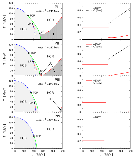
Figure 2: Left: $T-\mu$ phase diagrams for different model parameterizations. Solid (dashed) lines indicate first (second) order phase transitions. The dotted line is the lower spinodal corresponding to the homogeneous chiral restoration transition, while the dashed-dotted line is a boundary of a region in which there exists a local inhomogeneous minimum of the thermodynamical potential. TCP, LP and 3P stand for tricritical, Lifshitz and triple points. Right: values of $\phi$ and $Q$ as functions of the chemical potential, for $T=0$.

Let us start by analyzing the case of the parameterization PI (upper left panel of Fig. 2, corresponding to a relatively low chiral quark condensate $\langle\bar{q}q\rangle^{\rm ch}=-(240$ MeV$)^{3}$, and a relatively high value of the coupling $\bar{G}$). The different phases are indicated by the shaded areas, while solid and dashed lines correspond to first and second order transitions, respectively. At a temperature of about 100 MeV and low chemical potentials, it is seen that the system lies in the HCB phase, in which chiral symmetry is spontaneously broken. As usual, by increasing $\mu$ one finds a second order phase transition to an homogeneous phase in which chiral symmetry is restored (HCR phase). If the temperature is lowered, the corresponding second order transition curve ends at a tricritical point, beyond which it becomes a first order transition line. Now, by following this line, at a temperature $T_{3P}\simeq 20$ MeV one arrives at a triple point. For $T<T_{3P}$, at a given critical chemical potential $\mu_{c}(T)$ the system undergoes a first order transition from the HCB phase into an IH phase, in which chiral symmetry is found to be only approximately restored. On the other hand, if one starts with a system in the IH phase and increases the temperature at constant chemical potential, at some critical value of $T$ one arrives at a second order phase transition into the HCR phase. As it is shown in the figure, the corresponding second order transition line continues beyond the triple point with a dashed-dotted line inside the HCB area. The latter represents a boundary of a region in which the thermodynamic potential has a local minimum that corresponds to an (unstable) IH phase. Finally, in the phase diagram we also show with a dotted line the lower spinodal corresponding to the homogeneous chiral restoration transition.

The previously described first order transition from the HCB to the IH phase is illustrated in Fig. 3: left and right panels show contour plots of the mean field thermodynamic potential $\omega_{\mbox{\tiny MF}}^{\rm reg}(\phi,Q)$ at zero temperature for $\mu=260$ and $\mu=280$ MeV, respectively, which correspond to both sides of the transition point $\mu_{c}(0)=274$ MeV. The plots clearly show the transition from an absolute minimum at $\phi\simeq 340$ MeV, $Q=0$, to another one in which $\phi$ reduces to about 50 MeV, while the chiral condensates get spatial dependencies as those given by Eq. (17), with $Q\simeq 450$ MeV. These features are also shown in the upper right panel of Fig. 2, where we quote the curves for $\phi$ and $Q$ at $T=0$ as functions of the chemical potential. Notice that on the HCB side (left panel of Fig. 3) there also exists a local minimum at $(\phi,Q)\sim(50$ MeV, 400 MeV).

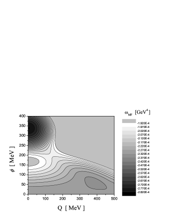
(a)

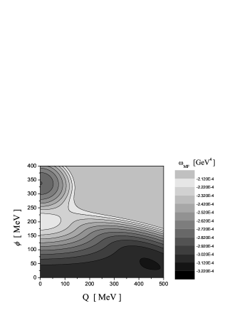
(b)

Figure 3: Contour plots of the thermodynamic potential $\omega^{\rm reg}_{\mbox{\tiny MF}}$ for a nonlocal chiral quark model at zero temperature and finite chemical potential, close to the first order transition between HCB and IH phases. The plots correspond to parameterization PI, for chemical potentials $\mu=260$ MeV (left) and $\mu=280$ MeV (right).

Below the previously discussed phase diagram we show in Fig. 2 the case of parameterization PII, in which the quark condensate at zero $T$ and $\mu$ is slightly larger, namely $\langle\bar{q}q\rangle^{\rm ch}=-(247$ MeV$)^{3}$. It can be seen that in this case the IH phase region gets reduced and splits in two: a small “island” of IH phase becomes isolated from the large IH phase “continent” found at high chemical potentials (see shaded regions in the figure). Then, for PIII and PIV it is seen that the island disappears, and the onset of the continent is pushed up to larger values of the chemical potential. The discontinuity of $Q$ at this transition for $T=0$ becomes increased, as it is shown in the right panels of Fig. 2. As stated above, for PIV (lower panels of Fig. 2) it is found that the inhomogeneous phase occurs for values of $\mu$ out of the region of the phase diagram displayed in our graphs. For comparison, in Table 1 we quote the values of the effective cutoffs, the values of $\phi$ and the chiral condensate $(-\langle\bar{q}q\rangle^{\rm ch})^{1/3}$ for zero $T$ and $\mu$, and the critical chemical potentials at $T=0$, for parameterizations PI to PIV. We denote by $\mu_{c}^{\prime}(0)$ the onset of the IH phase continent, while $\mu_{c}^{\prime\prime}(0)$ stands for the chemical potential at the transition between the IH phase island and the HCR phase region. All values are given in MeV.

	$(-\langle\bar{q}q\rangle^{\rm ch})^{1/3}$	$\Lambda$	$\phi$	$\mu_{c}(0)$	$\mu_{c}^{\prime\prime}(0)$	$\mu_{c}^{\prime}(0)$
PI	240	808	338	274	-	-
PII	247	863	315	266	288	295
PIII	270	1045	264	249	-	470
PIV	300	1295	227	236	-	629

Table 1: Effective cutoff $\Lambda$, chiral condensate and mean field $\phi$ at zero $T$ and $\mu$, and zero-temperature critical chemical potentials for parametrizations PI to PIV. All values are given in MeV.

It is worth pointing out that, for these models, the would-be Lifshitz point (i.e. the point where the HCB and HCR phases would meet the IH one along the second order phase transition lines) is hidden inside the HCB phase region: around the would-be LP, the HCB phase turns out to be energetically preferred in all cases considered. Instead, as it is indicated in the upper left panels of Fig. 2, a triple point can be found in the case of PI and PII. It is also worth mentioning that the second order phase transition curves, as well as both the TCP and would-be LP, can be calculated for these models through a quite precise semianalytical approach GomezDumm:2004sr ; Carlomagno:2014hoa .

The characteristics of the phase diagrams can be compared with those obtained within the NJL and the quark-meson model, which have been recently analyzed in this context. As stated in the Introduction, in the NJL the TCP and LP are coincident, whereas in the QM this can be the case or not, depending on the parameterization. In some cases it is shown Carignano:2014jla that the HCB-HCR second order phase transition ends at a Lifshitz point, while the TCP appears to be hidden into the IH region (i.e., the opposite situation to that found in our models). It is interesting to notice that, according to the analyses in Refs. Carignano:2011gr ; Carignano:2014jla ; Buballa:2014tba , for both the NJL and QM models some parameterizations lead to phase diagrams that show IH “continents” that extend to arbitrarily high chemical potentials. In fact, it is a matter of discussion whether the presence of these continents arises just as a regularization artifact. We stress that in nonlocal models the ultraviolet convergence of loop integrals follows from the behavior of form factors, which effectively embrace the underlying QCD interactions (indeed, the form factors can be fitted from lattice QCD calculations for the effective quark propagators Noguera:2008 ; Carlomagno:2013ona ). The fact that various quark models including different regularization procedures lead to similar qualitative features of the phase diagram seems to indicate that these features are rather robust. However, it is necessary to mention that we have not considered the effects of color superconductivity, which are expected to be important at intermediate and large chemical potentials and could have a significant impact in the phase diagram.

Finally, we address the case of instantaneous form factors mentioned in the previous section. For these parametrizations the qualitative features of the phase diagrams are found to be basically the same as those discussed above. The main difference is that similar diagrams correspond to models leading to larger values of the quark condensates: for a model with $(-\langle\bar{q}q\rangle^{\rm ch})^{1/3}=270$ MeV one obtains a phase diagram similar to that of parametrization PI for the covariant case, while the small “island” of inhomogeneous phase arises when the corresponding condensate is $(-\langle\bar{q}q\rangle^{\rm ch})^{1/3}\simeq 285$ MeV. For larger absolute values of the quark condensates the island disappears and the onset of the inhomogeneous phase is pushed up to larger values of the chemical potential, just as in the case of covariant form factors.

IV Summary and Conclusions

In this work we have analyzed the possible existence of inhomogeneous phases in the context of a simple version of nonlocal SU(2) chiral quark models in the chiral limit. For simplicity, only the one-dimensional modulation associated to a dual chiral density wave (DCDW) has been considered. In this framework, different parametrizations of the nonlocality, including both covariant and instantaneous form factors, have been investigated.

For all studied scenarios it is seen that the sizes of inhomogeneous phase regions show a rather strong dependence on model parameters. In all cases we find the existence of a tricritical point, while, keeping $f_{\pi}$ fixed, for high values of the dimensionless coupling $\bar{G}$ (low absolute values of the chiral condensate) we find at low temperatures a first order transition between the homogeneous chirally broken phase and the inhomogeneous phase. These phases and the homogeneous chirally restored one meet then at a triple point. On the other hand, for lower values of $\bar{G}$ the onset of the inhomogeneous phase is pushed up to higher chemical potentials and the triple point disappears. As in previous analyses made in the framework of NJL and QM models Carignano:2011gr ; Carignano:2014jla ; Buballa:2014tba , the inhomogeneous “continents” in our phase diagrams extend to arbitrarily high chemical potentials. Thus, their existence seems to be a rather robust prediction of this type of quark models. It should be mentioned, however, that effects of color superconductivity, which are expected to be important at intermediate and large chemical potentials, have not been included in these works. In this sense, it is clear that to clarify this issue color superconducting interaction channels have to be incorporated in future calculations. In addition, the role of vector channels within the framework of the nonlocal models deserves further investigation as well. Finally, it would be interesting to explore the possibility of going beyond the DCDW ansatz used in the present nonlocal scheme by considering more general one dimensional modulations.

References

- (1) For a recent review see M. Buballa and S. Carignano, Prog. Part. Nucl. Phys. 81, 39 (2015).
- (2) D. Nickel, Phys. Rev. Lett. 103, 072301 (2009); Phys. Rev. D 80, 074025 (2009).
- (3) U. Vogl and W. Weise, Prog. Part. Nucl. Phys. 27, 195 (1991); S. P. Klevansky, Rev. Mod. Phys. 64, 649 (1992); T. Hatsuda and T. Kunihiro, Phys. Rept. 247, 221 (1994).
- (4) S. Carignano, M. Buballa and B. J. Schaefer, Phys. Rev. D 90, 014033 (2014).
- (5) J. P. Carlomagno, D. G. Dumm and N. N. Scoccola, Phys. Lett. B 745, 1 (2015).
- (6) T. Schafer and E. V. Shuryak, Rev. Mod. Phys. 70, 323 (1998).
- (7) C. D. Roberts and A. G. Williams, Prog. Part. Nucl. Phys. 33 (1994) 477; C. D. Roberts and S. M. Schmidt, Prog. Part. Nucl. Phys. 45, S1 (2000).
- (8) S. Noguera and N. N. Scoccola, Phys. Rev. D 78, 114002 (2008).
- (9) P. O. Bowman, U. M. Heller, and A. G. Williams, Phys. Rev. D 66, 014505 (2002); P. O. Bowman, U. M. Heller, D. B. Leinweber and A. G. Williams, Nucl. Phys. Proc. Suppl. 119, 323 (2003).
- (10) M. B. Parappilly, P. O. Bowman, U. M. Heller, D. B. Leinweber, A. G. Williams and J. B. Zhang, Phys. Rev. D 73, 054504 (2006).
- (11) S. Furui and H. Nakajima, Phys. Rev. D 73, 074503 (2006).
- (12) G. Ripka, Quarks bound by chiral fields (Oxford University Press, Oxford, 1997).
- (13) R.D. Bowler and M.C. Birse, Nucl. Phys. A 582, 655 (1995); R.S. Plant and M.C. Birse, Nucl. Phys. A 628, 60 (1998).
- (14) S. M. Schmidt, D. Blaschke and Y. L. Kalinovsky, Phys. Rev. C 50, 435 (1994).
- (15) B. Golli, W. Broniowski and G. Ripka, Phys. Lett. B 437, 24 (1998); W. Broniowski, B. Golli and G. Ripka, Nucl. Phys. A 703, 667 (2002).
- (16) D. Gomez Dumm and N.N. Scoccola, Phys. Rev. D 65, 074021 (2002).
- (17) A. Scarpettini, D. Gomez Dumm and N.N. Scoccola, Phys. Rev. D 69, 114018 (2004).
- (18) D. Gomez Dumm and N. N. Scoccola, Phys. Rev. C 72, 014909 (2005).
- (19) D. Gomez Dumm, A. G. Grunfeld and N.N. Scoccola, Phys. Rev. D 74, 054026 (2006).
- (20) T. Hell, S. Roessner, M. Cristoforetti and W. Weise, Phys. Rev. D 79, 014022 (2009).
- (21) G. A. Contrera, D. Gomez Dumm and N. N. Scoccola, Phys. Rev. D 81, 054005 (2010).
- (22) T. Hell, S. Rossner, M. Cristoforetti and W. Weise, Phys. Rev. D 81, 074034 (2010).
- (23) G. A. Contrera, M. Orsaria and N. N. Scoccola, Phys. Rev. D 82, 054026 (2010).
- (24) D. Gomez Dumm, S. Noguera and N.N. Scoccola, Phys. Lett. B 698, 236 (2011); Phys. Rev. D 86, 074020 (2012).
- (25) V. Pagura, D. Gomez Dumm and N. N. Scoccola, Phys. Lett. B 707, 76 (2012).
- (26) J. P. Carlomagno, D. Gómez Dumm and N. N. Scoccola, Phys. Rev. D 88, 074034 (2013).
- (27) E. Nakano and T. Tatsumi, Phys. Rev. D 71, 114006 (2005).
- (28) D. Müller, M. Buballa and J. Wambach, Phys. Lett. B 727, 240 (2013).
- (29) S. Aoki et al., Eur. Phys. J. C 74, no. 9, 2890 (2014).
- (30) H. Grigorian, Phys. Part. Nucl. Lett. 4, 223 (2007).
- (31) S. Carignano and M. Buballa, Acta Phys. Polon. Supp. 5, 641 (2012).
- (32) R. T. Cahill and C. D. Roberts, Phys. Rev. D 32, 2419 (1985); J. Praschifka, C. D. Roberts and R. T. Cahill, Phys. Rev. D 36, 209 (1987).