Approximate Greedy Clustering and Distance Selection for Graph Metrics

Abstract

In this paper, we consider two important problems defined on finite metric spaces, and provide efficient new algorithms and approximation schemes for these problems on inputs given as graph shortest path metrics or high-dimensional Euclidean metrics. The first of these problems is the greedy permutation (or farthest-first traversal) of a finite metric space: a permutation of the points of the space in which each point is as far as possible from all previous points. We describe randomized algorithms to find $(1+{\varepsilon})$-approximate greedy permutations of any graph with $n$ vertices and $m$ edges in expected time $O\left({{\varepsilon}^{-1}(m+n)\log n\log(n/{\varepsilon})}\right)$, and to find $(1+{\varepsilon})$-approximate greedy permutations of points in high-dimensional Euclidean spaces in expected time $O({\varepsilon}^{-2}n^{1+1/(1+{\varepsilon})^{2}+o(1)})$. Additionally we describe a deterministic algorithm to find exact greedy permutations of any graph with $n$ vertices and treewidth $O(1)$ in worst-case time $O(n^{3/2}\log^{O(1)}n)$. The second of the two problems we consider is distance selection: given $k\in\left\llbracket\binom{n}{2}\right\rrbracket$, we are interested in computing the $k$th smallest distance in the given metric space. We show that for planar graph metrics one can approximate this distance, up to a constant factor, in near linear time.

1 Introduction

In this paper we are interested in several important algorithmic problems on finite metric spaces, including the construction of greedy permutations, the problem of selecting the $k$th distance among all pairs of points in the space, and the problem of counting the number of points in a metric ball. These problems have known polynomial time algorithms (for instance, the $k$th distance may be found by applying a selection algorithm to the coefficients of the distance matrix); however, we are interested in algorithms that scale well to large data sets, so we seek algorithms that take subquadratic time (substantially smaller than the time to list all distances). To achieve this, we require the metric space to be defined implicitly, for instance as the distances in a sparse weighted graph or as the distances among points in a Euclidean metric space. Despite the increased difficulty of working with implicit metrics, we show that the problems we study can be solved efficiently.

1.1 Greedy permutation

In the first sections of this paper we are interested in an ordering problem on metric spaces: the construction of greedy permutations. We solve this problem exactly and approximately, for the shortest path metrics of sparse weighted graphs and for high-dimensional Euclidean spaces.

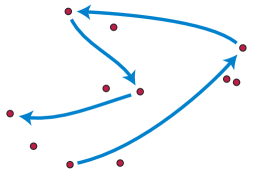
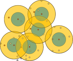
Figure 1: Left: The first five points of a greedy permutation. Each point is as far as possible from all previously chosen points. Right: The six red points at the centers of the disks form an $r$-net of the set $V$ of red and white points, where $r$ is the radius of the large yellow disks. The darker disks of radius $r/2$ are disjoint from each other, and the disks of radius $r$ together cover all of $V$.

     (A)

     (B)

     (C)

     (D)

     (E)

     (F)

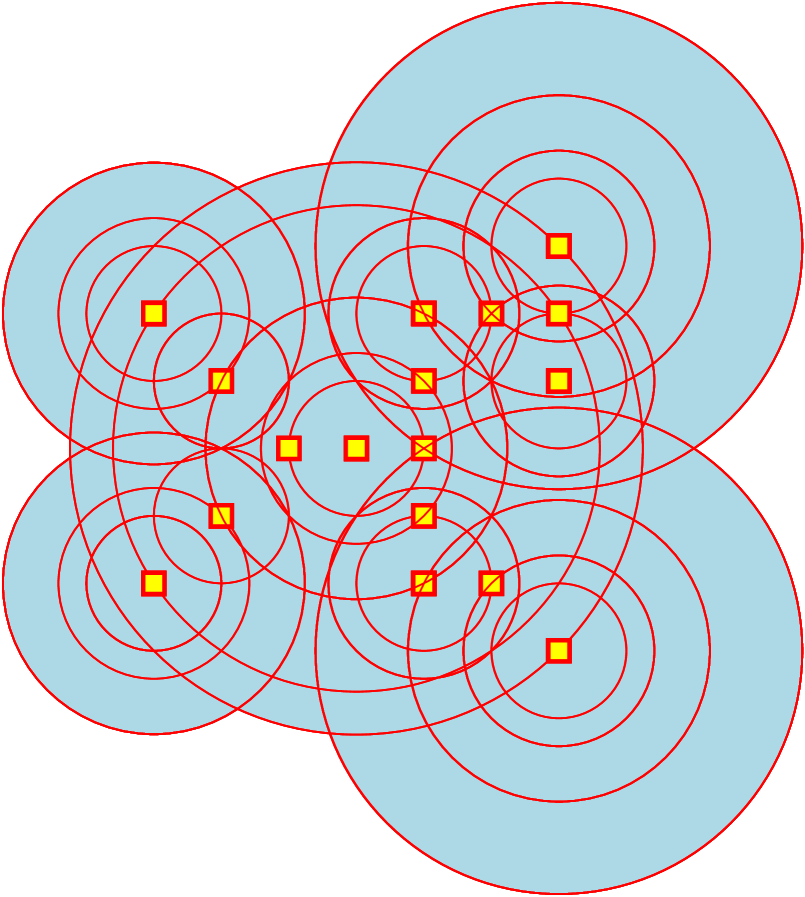
     (G)

Figure 2: (A) A point set. (B)–(G) The different representations of this point set as a union of balls, as provided by different prefixes of the greedy permutation. As this demonstrates, one can think about a prefix of the greedy permutation as a partial representation of the point set that keeps improving as the prefix used gets longer.

A permutation $\Pi=\left\langle{\pi_{1},\pi_{2},\ldots}\right\rangle$ of the vertices of a metric space $(V,d)$ is a greedy permutation (also called a farthest-first traversal or farthest point sampling) if each vertex $\pi_{i}$ is the farthest in $V$ from the set $\Pi_{i-1}=\left\{{\pi_{1},\ldots,\pi_{i-1}}\right\}$ of preceding vertices (Figure 1, left). Greedy permutations were introduced by Rosenkrantz et al. [RSL77] for the “farthest insertion” traveling salesman heuristic, and used by Gonzalez [Gon85] to 2-approximate the $k$-center. Different prefixes of the greedy permutation provide different multi-resolution clusterings of the input point set; see Figure 2${}_{\text{p\ref{fig:multi:resolution}}}$.

Greedy permutations are closely related to another concept for finite metric spaces, $r$-nets. An $r$-net for the metric space $(V,d)$ and the numerical parameter $r$ is a subset $\mathcal{N}$ of the points of $V$ such that no two of the points of $\mathcal{N}$ are within distance $r$ of each other, and such that every point of $V$ is within distance $r$ of a point of $\mathcal{N}$. Equivalently, the closed $r/2$-balls centered at the points of $\mathcal{N}$ are disjoint, and the closed $r$-balls around the same points cover all of $V$ (Figure 1, right). Each prefix of a greedy permutation is an $r$-net, for $r$ equal to the minimum distance between points in the prefix, and for every $r$ an $r$-net may be obtained as a prefix of a greedy permutation.

Greedy permutations may be computed for metric spaces in $O(n^{2})$ time, and for graphs in the same time as all pairs shortest paths, by a naive algorithm (Section 2) that maintains the distances of all points from the selected points. The only previous improvement on the naive algorithm, by Har-Peled and Mendel [HM06] defines a concept of approximation for greedy permutations that we will also use. They showed that $(1+{\varepsilon})$-greedy permutations can be computed in $O(n\log n)$ time in metric spaces with constant doubling dimension; these are permutations $\Pi=\left\langle{\pi_{1},\pi_{2},\ldots}\right\rangle$ for which there exists a sequence of numbers $r_{1}\geq r_{2}\geq\cdots$ such that

1. the maximum distance of a point of $V$ from $\Pi_{i}$ is in the range $\left[{r_{i},\,(1+{\varepsilon})r_{i}}\rule[-5.69046pt]{0.0pt}{11.38092pt}\right]$, and

2. the distance between every two points $u,v\in\Pi_{i}$ is at least $r_{i}$.

In this paper we give approximation schemes for metric spaces defined by sparse graphs, and high-dimensional Euclidean spaces, neither of which have constant doubling dimension. Greedy permutations for graph distances were previously mentioned by Gu et al. [GJG11], in connection with an application in molecular dynamics, but rejected by them because the naive algorithm was too slow.

One reason for interest in greedy or $(1+{\varepsilon})$-greedy permutations is that, in a single structure, they approximate an optimal clustering for all possible resolutions. Specifically, the prefix of the first $k$ vertices in such a permutation, provides, for any $k$, a $2(1+{\varepsilon})$-approximation to the optimal $k$-center clustering of ${G}$. (See Lemma 2.1 for an easy proof of this.) The $k$-center problem may be 2-approximated in $O(kn)$ time by computing the first $k$ vertices of a greedy permutation, and is NP-hard to approximate to a ratio better than 2 [Gon85]. For points in Euclidean spaces of bounded dimension a linear-time 2-approximation is known [Har04, HR13]. Thorup [Tho05] provided a fast $k$-center approximation for graph shortest path metrics with a single choice of $k$. The $k$-center problem may be solved exactly on trees and cactus graphs in $O(n\log n)$ time [FJ83]. Voevodski et al. [VBR⁺10] use an algorithm closely related to greedy permutation to approximate a different clustering problem, $k$-medians.

Intuitively, every prefix of a greedy permutation is as informative as possible about the whole set, so greedy permutations form a natural ordering in which to stream large data sets. Because of these properties, greedy permutations have many additional applications, including color quantization [Xia97], progressive image sampling [ELPZ97], selecting landmarks of probabilistic roadmaps for motion planning [MAB98], point cloud simplification [MD03], halftone mask generation [SMR04], hierarchical clustering [DL05], detecting isometries between surface meshes [LF09], novelty detection and time management for autonomous robot exploration [GGD12], industrial fault detection [AYE12], and range queries seeking diverse sets of points in query regions [AAYI⁺13].

1.2 Distance selection and approximate range counting

The distance selection problem, in computational geometry, has as input a set of points in $\mathbb{R}^{d}$; the output is the $k$th smallest distance defined by a pair of points of $P$. It is believed that such exact distance selection requires $\Omega\left({n^{4/3}}\right)$ time in the worst case [Eri95], even in the plane (in higher dimensions the bound deteriorates). Recently, Har-Peled and Raichel [HR13] provided an algorithm that $(1+{\varepsilon})$-approximates this distance in $O(n/{\varepsilon}^{d})$ time.

We are interested in solving the problem for the finite metric case. Specifically, consider a shortest path metric defined over a graph ${G}$ with $n$ vertices and $m$ edges. Given $k\in\left\llbracket\binom{n}{2}\right\rrbracket=\left\{{1,\ldots,\binom{n}{2}}\right\}$, we would like to compute the $k$th smallest distance in this shortest path metric. This problem was studied for trees [MTZC81], where Frederickson and Johnson [FJ83] provided a beautiful algorithm that works by using tree separators, and selection in sorted matrices [FJ84].

The “dual” problem to distance selection is distance counting. Here, given a distance $r$, the task is to count the number of pairs of points of $P$ that are of distance $\leq r$. While the problems are essentially equivalent in the exact case, approximate distance counting seems to be significantly easier than selection.

Throughout this paper, ${G}=(V,E)$ will denote an undirected graph with $n$ vertices and $m$ edges, with non-negative edge weights that obey the triangle inequality. The shortest path distances in ${G}$ induce a metric $d$. Specifically, for any $u,v\in V$, let ${d}_{G}\left({u,v}\right)$ denotes the shortest path between $u$ and $v$ in ${G}$. Given a graph ${G}=(V,E)$, and a query distance $r$, the set of $r$-short pairs is

$$P_{\leq{r}}=\left\{\Bigl{.}\left\{{u,v}\right\}\subseteq V\;\middle|\;u\neq v\text{ and }{d}_{G}\left({u,v}\right)\leq r\right\}.$$ (1)

In the distance counting problem, the task is to compute (or approximate) $\left|{P_{\leq r}}\right|$. In the distance selection problem, given $k\in\left\llbracket\binom{n}{2}\right\rrbracket$, the task is to compute (or approximate) the smallest $r$ such that $\left|{P_{\leq{r}}}\right|\geq k$.

Distance counting is easy to approximate using known techniques, since this problem is malleable to random sampling, see [Coh14] and references therein. However, approximate distance selection is significantly harder, as random sampling can not be used in this case – indeed, trying to use approximate distance counting (or sketches approach as in [Coh14]), may result in an arbitrarily bad approximation to the $k$th distance, if the $(k-1)$th and $(k+1)$th distance are significantly smaller and larger, respectively, than the $k$th distance (or similar sparse scenarios).

1.3 New results

Greedy permutation for sparse graphs.

In Section 2, we show that an $(1+{\varepsilon})$-greedy permutation can be found for graphs with $n$ vertices and $m$ edges in time $O\left({{\varepsilon}^{-1}m\log n\log(n/{\varepsilon})}\right)=\widetilde{O}\left({m}\right)$.

Approximate greedy permutation for high dimensional Euclidean space.

In Section 3, we show that an approximate greedy permutation can be computed for a set of points in high-dimensional Euclidean space. The algorithm runs in subquadratic time and has polynomial dependency on the dimension. Our approximations are based on finding $r$-nets (or in the Euclidean case approximate $r$-nets) for a geometric sequence of values of $r$

In an earlier paper [HIS13], the authors showed that for high dimensional point sets one can get a sparse spanner. Applying the above algorithm for sparse graphs to this spanner yields a greedy permutation, but with significantly weaker bounds, as the stretch in the constructed spanner is at lease $2$.

Exact greedy permutation for bounded tree-width.

In Section 4, we show how to find an exact greedy permutation for graphs of bounded treewidth, in time $\widetilde{O}\left({n^{3/2}}\right)$, by partitioning the input graph into small subgraphs separated from the rest of the graph by $O(1)$ vertices, and by using an orthogonal range searching data structure in each subgraph to find the farthest vertex from the already-selected vertices.

Distance selection in planar graphs.

In Section 5, we show how to $O(1)$-approximate the $k$th distance in a planar graph ${G}$. Specifically, given $k$, the algorithm computes in near linear time, a number $\alpha$, such that the $k$th shortest distance in ${G}$ is at least $\alpha$, and at most $O(\alpha)$. This algorithm uses a planar separator and distance oracles in an interesting way to count distances.

2 Approximate greedy permutation on a sparse graph

We are interested in approximating the greedy permutation for a graph ${G}$. Among other motivations, this provides a good approximation for $k$-center clustering:

Lemma 2.1.

If $\Pi$ is a $(1+{\varepsilon})$-greedy permutation of $\mathcal{M}=(V,d)$, then, for all $k$, $\Pi_{k}$ provides a $2(1+{\varepsilon})$-approximation to the optimal $k$-center clustering and minimax diameter $k$-clustering of $\mathcal{M}$.

Proof:

By Property (A) of such a permutation (see Section 1.1), all points of $V$ can be covered by balls of radius $(1+{\varepsilon})r_{k}$ centered at $\pi_{1},\ldots,\pi_{k}$; these balls have diameter $\leq 2(1+{\varepsilon})r_{k}$. Let $S=\Pi_{k}\cup\left\{{v}\right\}$, where $v$ is the farthest point in $V$ from $\Pi_{k}$. By the definition of $r_{i}$ and by Property (B) of these permutations, every two points in $S$ have distance at least $r_{i}$, so no $k$ clusters of radius smaller than $r_{i}/2$ or diameter smaller than $r_{i}$ can cover the $k+1$ points in $S$.

A naive algorithm for computing the greedy permutation maintains for each vertex $v$ its distance $\mathrm{\ell}_{v}$ to the set of centers picked so far, and uses these distances as priorities in a max-heap, which it uses to select each successive center, using Dijkstra’s algorithm to update the distances after each center is picked. There are $n$ instantiations of Dijkstra’s algorithm, taking time $O(n(m+n\log n))$.

To improve performance, we may avoid adding a vertex $v$ to the min-heap used within Dijkstra’s algorithm unless its tentative distance is smaller than $\mathrm{\ell}_{v}$, preventing the expansion of vertices for which the distance from $v_{i}$ is no smaller than $\mathrm{\ell}_{v}$. This idea does not immediately improve the worst-case running time of the algorithm but will be important in our approximation algorithm.

2.1 Computing an $r$-net in a sparse graph

We compute an $r$-net in a sparse graph using a variant of Dijkstra’s algorithm with the sequence of starting vertices chosen in a random permutation. A similar idea was used by Mendel and Schwob [MS09] for a different problem; however, using this method for our problem involves a more complicated analysis.

Let ${G}=(V,E)$ be a weighted graph with $n$ vertices and $m$ edges, let $r>0$, and let $\pi_{i}$ be the $i$th vertex in a random permutation of $V$. For each vertex $v$ we initialize $\delta(v)$ to $+\infty$. In the $i$th iteration, we test whether $\delta(\pi_{i})\geq r$, and if so we do the following steps:

1. Add $\pi_{i}$ to the resulting net $\mathcal{N}$.

2. Set $\delta(\pi_{i})$ to zero.

3. Perform Dijkstra’s algorithm starting from $\pi_{i}$, modified as in Section 2to avoid adding a vertex $u$ to the priority queue unless its tentative distance is smaller than the current value of $\delta(u)$. When such a vertex $u$ is expanded, we set $\delta(u)$ to be its computed distance from $\pi_{i}$, and relax the edges adjacent to $u$ in the graph.

The difference from the algorithm of Mendel and Schwob is that their algorithm initiates an instance of Dijkstra’s algorithm starting from every vertex $\pi_{i}$, whereas we do so only when $\delta(\pi_{i})\geq r$.

Lemma 2.2.

The set $\mathcal{N}$ is an $r$-net in ${G}$.

Proof:

By the end of the algorithm, each $v\in V$ has $\delta(v)<r$, for $\delta(v)$ is monotonically decreasing, and if it were larger than $r$ when $v$ was visited then $v$ would have been added to the net.

An induction shows that if $\ell=\delta(v)$, for some vertex $v$, then the distance of $v$ to the set $\mathcal{N}$ is at most $\ell$. Indeed, for the sake of contradiction, let $j$ be the (end of) the first iteration where this claim is false. It must be that $\pi_{j}\in\mathcal{N}$, and it is the nearest vertex in $\mathcal{N}$ to $v$. But then, consider the shortest path between $\pi_{j}$ and $v$. The modified Dijkstra must have visited all the vertices on this path, thus computing $\delta(v)$ correctly at this iteration, which is a contradiction.

Finally, observe that every two points in $\mathcal{N}$ have distance $\geq r$. Indeed, when the algorithm handles vertex $v\in\mathcal{N}$, its distance from all the vertices currently in $\mathcal{N}$ is $\geq r$, implying the claim.

Lemma 2.3.

Consider an execution of the algorithm, and any vertex $v\in V$. The expected number of times the algorithm updates the value of $\delta(v)$ during its execution is $O(\log n)$, and more strongly the number of updates is $O(\log n)$ with high probability.

Proof:

For simplicity of exposition, assume all distances in ${G}$ are distinct. Let $S_{i}$ be the set of all the vertices $x\in V$, such that the following two properties both hold:

1. $d\left({x,v}\right)<d\left({v,\Pi_{i}}\right)$, where $\Pi_{i}=\left\{{\pi_{1},\ldots,\pi_{i}}\right\}$.

2. If $\pi_{i+1}=x$ then $\delta(v)$ would change in the $(i+1)$th iteration.

Let $s_{i}=\left|{S_{i}}\right|$. Observe that $S_{1}\supseteq S_{2}\supseteq\cdots\supseteq S_{n}$, and $\left|{S_{n}}\right|=0$.

In particular, let $\mathcal{E}_{i+1}$ be the event that $\delta(v)$ changed in iteration $(i+1)$ – we will refer to such an iteration as being active. If iteration $(i+1)$ is active then one of the points of $S_{i}$ is $\pi_{i+1}$. However, $\pi_{i+1}$ has a uniform distribution over the vertices of $S_{i}$, and in particular, if $\mathcal{E}_{i+1}$ happens then $s_{i+1}\leq s_{i}/2$, with probability at least half, and we will refer to such an iteration as being lucky. (It is possible that $s_{i+1}<s_{i}$ even if $\mathcal{E}_{i+1}$ does not happen, but this is only to our benefit.) After $O(\log n)$ lucky iterations the set $S_{i}$ is empty, and we are done. Clearly, if both the $i$th and $j$th iteration are active, the events that they are each lucky are independent of each other. By the Chernoff inequality, after $c\log n$ active iterations, at least $\left\lceil{\log_{2}n}\right\rceil$ iterations were lucky with high probability, implying the claim. Here $c$ is a sufficiently large constant.

Interestingly, in the above proof, all we used was the monotonicity of the sets $S_{1},\ldots,S_{n}$, and the fact that if $\delta(v)$ changes in an iteration then the size of the set $S_{i}$ shrinks by a constant factor with good probability in this iteration. This implies that there is some flexibility in deciding whether or not to initiate Dijkstra’s algorithm from each vertex of the permutation, without damaging the number of times of the values of $\delta(v)$ are updated. We will use this flexibility later on.

Lemma 2.4.

Given a graph ${G}=(V,E)$, with $n$ vertices and $m$ edges, the above algorithm computes an $r$-net of ${G}$ in $O((n+m)\log n)$ expected time.

Proof:

By Lemma 2.3, the two $\delta$ values associated with the endpoints of an edge get updated $O(\log n)$ times, in expectation, during the algorithm’s execution. As such, a single edge creates $O(\log n)$ decrease-key operations in the heap maintained by the algorithm. Each such operation takes constant time if we use Fibonacci heaps to implement the algorithm.

2.2 An approximation whose time depends on the spread

Given a finite metric space $(V,d)$ defined over a set $V$, its spread is the ratio between the maximum and minimum distance in the metric; formally,

$$\mathrm{spread}\left({d}\right)=\max_{{u,v\in V,u\neq v}}{d}_{G}\left({u,v}\right)/\min_{{u,v\in V,u\neq v}}{d}_{G}\left({u,v}\right).$$

Let graph ${G}=(V,E)$ and ${\varepsilon}>0$ be given. Assume for now that the minimum edge length is $1$, and that the diameter of ${G}$ is at most $\Delta$. Set $r_{i}=\Delta/(1+{\varepsilon})^{i-1}$, for $i=1,\ldots,M=\left\lceil{\log_{1+{\varepsilon}}\Delta}\right\rceil$. We compute a sequence of nets in a sequence of iterations. In the first iteration, compute an $r_{1}$-net $\mathcal{N}_{1}$ of ${G}$, using Lemma 2.4. In the beginning of the $i$th iteration, for $i>1$, let $\mathcal{S}_{i}=\cup_{j<i}\mathcal{N}_{i}$. Using Dijkstra, mark as used all vertices within distance $r_{i}$ of $\mathcal{S}_{i}$. Compute an $r_{i}$-net $\mathcal{N}_{i}$ in ${G}$, modifying the algorithm of Lemma 2.4 by disallowing used vertices from being considered as net points.

After completing these computations, combine the vertices into a single permutation in which the vertices of $\mathcal{N}_{i}$ form the $i$th contiguous block. Within this block, the ordering of the vertices of $\mathcal{N}_{i}$ is arbitrary. The following is easy to verify, and we omit the easy proof.

Lemma 2.5.

Let $\mathcal{N}=\mathcal{N}_{1}\cup\cdots\cup\mathcal{N}_{t}$, for an arbitrary $t$. Then the distance of every vertex $v\in{G}$ from $\mathcal{N}$ is at most $r_{t}$, and the distance between any pair of vertices of the net is at least $r_{t}$.

That is, the net computed by the $t$th iteration is a “perfect” $r_{t}$ net. In between such blocks, it might be less then perfect. Formally, we have the following (again, we omit the relatively easy proof).

Lemma 2.6.

Let $\pi$ be the permutation computed by the above algorithm, and consider the $i$th vertex $\pi_{i}$ in this permutation. Assume that $\pi_{i}\in\mathcal{N}_{t}$. Then we have the following guarantees:

1. The distance between any two vertices of $\Pi_{i}=\left\{{\pi_{1},\ldots,\pi_{i}}\right\}$ is at least $r_{t}$.

2. The distance of any vertex of $v\in V$ from $\Pi_{i}$, is at most $r_{t-1}=(1+{\varepsilon})r_{t}$.

Lemma 2.7.

Let ${G}=(V,E)$ be a graph, let ${\varepsilon}>0$, and let $\Phi$ be the spread of ${G}$. Then, one can compute a $(1+{\varepsilon})$-greedy permutation in $O\left({{\varepsilon}^{-1}\left({n+m}\right)\log n\log\Phi}\right)$ expected time.

Proof:

A $2$-approximation to the diameter of ${G}$ can be found by running Dijkstra’s algorithm from an arbitrary starting vertex. The minimum distance in ${G}$ is achieved by an edge (since the edge weights are positive), so it can be computed in linear time. After scaling, we can use the above algorithm, with $M=O\left({\log_{1+{\varepsilon}}\Phi}\right)=O\left({{\varepsilon}^{-1}\log\Phi}\right)$ iterations, each using a modified version of the algorithm of Section 2.1. It is straightforward to modify the analysis to show that the each such iteration takes $O((n+m)\log n)$ time in expectation.

2.3 Eliminating the dependence on the spread

An arbitrary graph ${G}$ may not have small enough spread to apply the previous algorithm directly. In this case, following by-now standard methods for eliminating the dependence on spread (see Section 4 of [MS09]), we simulate the algorithm more efficiently, using a value of ${\varepsilon}$ smaller by a constant factor to make up for some additional approximation in our simulation.

Consider an iteration of the above algorithm for distance $r_{i}$. Edges longer than $nr_{i}$ can be ignored or (conceptually) deleted, as they cannot be used by the $r$-net algorithm of Section 2.1. Similarly, edges of length $O\left({{\varepsilon}r_{i}/n^{2}}\right)$ can be collapsed and treated as having length zero. Thus, an edge $e$ of length $\ell$ is active when $r_{i}$ is in the interval $\!\!\left[{\frac{c{\varepsilon}\ell}{n^{2}},\ell n}\rule[-5.69046pt]{0.0pt}{11.38092pt}\right]$, which happens for $O\left({\log_{1+{\varepsilon}}(n^{3}/{\varepsilon})}\right)=O\left({{\varepsilon}^{-1}\log(n/{\varepsilon})}\right)$ iterations. Let $m_{i}$ be the number of active edges in the $i$th iteration, and let ${G}_{i}$ be the resulting graph, in which all the edges of lengths $\leq{\varepsilon}r_{i}/n^{2}$ are contracted (the resulting super vertex is identified with one of the original vertices), and all the edges of length $>r_{i}n$ are removed. Any singleton vertex in this graph is not relevant for computing the permutation in this resolution, and it can be ignored. The running time of Lemma 2.4 on ${G}_{i}$ is $O\left({m_{i}\log m_{i}}\right)$.

When the algorithm moves to the next iteration, it needs to introduce into ${G}_{i}$ all the new edges that become active. Using a careful implementation, this can be done in $O(1)$ amortized time, for any newly introduced edge. Similarly, edges that become inactive should be deleted. Of course, if there are no active edges, the algorithm can skip directly to the next resolution. This can be easily done, by putting the edges into a heap, sorted by their length, and adding the edges and removing them as the algorithm progresses down the resolutions.

The overall expected running time of this algorithm is $O\left({\sum_{i}m_{i}\log m_{i}+m\log m}\right)$. However, since every edge is active in $O\left({{\varepsilon}^{-1}\log(n/{\varepsilon})}\right)$ iterations, we get that the expected running time is $O\left({{\varepsilon}^{-1}m\log n\log(n/{\varepsilon})}\right)$. We thus get the following.

Theorem 2.8.

Given a non-negatively weighted graph ${G}=(V,E)$, with $n$ vertices and $m$ edges, and a parameter ${\varepsilon}>0$, one can compute a $(1+{\varepsilon})$-approximate greedy permutation for ${G}$ in expected time $O\left({{\varepsilon}^{-1}m\log n\log(n/{\varepsilon})}\right)$.

2.4 $k$-center clustering for bounded spread with integer weights

Our greedy permutation algorithm for sparse graphs leads to a fast $(2+\epsilon)$-approximation to the $k$-center problem for graph metrics. In this case, it is possible to eliminate the dependence on $\epsilon$, giving a $2$-approximation (best possible as achieving a smaller approximation ratio is NP-hard).

Theorem 2.9.

Let ${G}$ be a graph with $n$ vertices and $m$ edges, with positive integer weights on the edges, and spread $\Phi$. Given $k$, one can compute a $2$-approximation to the optimal $k$-center clustering of ${G}$, in $O\left({m\log n\log\Phi}\right)$ time both in expectation and with high probability.

Proof:

Using Dijkstra’s algorithm starting from an arbitrary vertex in ${G}$, compute, in $O(m+n\log n)$ time, a number $\Delta$, such that $\mathrm{diam}\left({{G}}\right)\leq\Delta\leq 2\mathrm{diam}\left({{G}}\right)$. We next perform a binary search for the radius $r_{\mathrm{opt}}$ of the optimal $k$-center clustering of ${G}$, in the range $1,\ldots,\Delta$.

Given a candidate radius $x$, let $r=2x$ and compute an $r$-net of ${G}$ using the algorithm of Lemma 2.4. It is easy to verify that if $x\geq r_{\mathrm{opt}}$, then the resulting net $\mathcal{N}$ has at most $k$ vertices in it. Indeed, consider all the vertices in ${G}$ assigned to a single cluster $C$ in the optimal $k$-center clustering, and observe that $\mathrm{diam}\left({C}\right)\leq 2r_{\mathrm{opt}}\leq r$. Therefore, at most one vertex of $C$ may belong to any $r$-net, so every $r$-net for this value of $r$ has at most $k$ vertices. On the other hand, if $x$ is too small then the resulting $r$-net has more then $k$ vertices.

Thus, using the $r$-net procedure of Lemma 2.4 as a decider in a binary search yields the desired approximation algorithm.

3 Approximate greedy permutation on Euclidean metrics

3.1 Approximate nets

Lemma 3.1 (Johnson–Lindenstrauss lemma [JL84]).

For any ${\varepsilon}>0$, every set of $n$ points in Euclidean space admits an embedding into $(\mathbb{R}^{O(\log n/{\varepsilon}^{2})},\|\cdot\|_{2})$, with distortion $1+{\varepsilon}$.

Definition 3.2.

Let $H$ be a family of hash functions mapping $\mathbb{R}^{d}$ to some universe $U$. We say that $H$ is $(\delta,c\delta,p_{1},p_{2})$-sensitive if for any $x,y\in\mathbb{R}^{d}$ it satisfies the following properties:

1. If $\|x-y\|_{2}\leq\delta$ then $\Pr_{h\in H}[h(x)=h(y)]\geq p_{1}$.

2. If $\|x-y\|_{2}\geq c\delta$ then $\Pr_{h\in H}[h(x)=h(y)]\leq p_{2}$.

Lemma 3.3 (Andoni & Indyk [AI06]).

For any $\delta>0$, dimension $d>0$, and $c>1$, there exists a $\left({\delta,c\delta,1/n^{1/c^{2}+o(1)},1/n}\right)$-sensitive family of hash functions for $\mathbb{R}^{d}$, where every function can be evaluated in time $O\left({d\cdot n^{o(1)}}\right)$.

We extend the notion of nets to $c$-approximate $r$-nets, for $c\geq 1$, $r>0$, and metric space $(V,d)$. These are subsets $\mathcal{N}$ of the points of $V$ such that no two of the points of $\mathcal{N}$ are within distance $r$ of each other, and such that every point of $V$ is within distance $c\cdot r$ of a point of $\mathcal{N}$.

Theorem 3.4.

Let $d>0$, $r>0$, ${\varepsilon}>0$. Given a set $X$ of $n$ points in $\mathbb{R}^{d}$, one can compute in expected running time $O\left({{\varepsilon}^{-2}n^{1+1/(1+{\varepsilon})^{2}+o(1)}}\right)$ a set $\mathcal{N}\subseteq X$ such that $\mathcal{N}$ is a $(1+{\varepsilon})$-approximate $r$-net for the Euclidean metric on $X$ with high probability.

Proof:

By Lemma 3.1 we may assume that $d=O\left({\log n/{\varepsilon}^{2}}\right)$, since otherwise we can embed $X$ into Euclidean space of dimension $O\left({\log n/{\varepsilon}^{2}}\right)$, with distortion $1+O({\varepsilon})$. Any $\left({1+O({\varepsilon})}\right)$-approximate $r$-net for this new point set is a $\left({1+O({\varepsilon})}\right)$-approximate $r$-net for $X$.

Let $c=1+{\varepsilon}$. Let $H$ be the $(r,cr,p_{1},p_{2})$-sensitive family of hash functions given by Lemma 3.3, with $p_{1}=1/n^{1/c^{2}+o(1)}$, $p_{2}=1/n$. We sample $k=O\left({(1/p_{1})\cdot\log n}\right)=O\left({n^{1/c^{2}+o(1)}}\right)$ hash functions $h_{1},\ldots,h_{k}\in H$. For every $i\in\{1,\ldots,k\}$, and for every $x\in X$, we evaluate $h_{i}(x)$.

We construct a set $\mathcal{N}\subseteq X$ which is initially empty, and it will be the desired net at the end of the algorithm. Initially, we consider all points in $X$ as being unmarked. We pick an arbitrary ordering $x_{1},\ldots,x_{n}$ of the points in $X$, and we iterate over all points in this order. When the iteration reaches point $x_{i}$, if it is already marked, we skip it, and continue with the next point. Otherwise, we add $x_{i}$ to $\mathcal{N}$, and we proceed as follows. Let $M_{i}$ be the set of all currently marked points. Let $S_{i}=\bigcup_{j=1}^{k}h_{j}^{-1}(x_{i})\setminus M_{i}$ be the set of unmarked points that are hashed to the same value in at least one of the sampled hash functions $h_{1},\ldots,h_{k}$. We mark all points $y\in S_{i}$, such that $\|x_{i}-y\|_{2}\leq c\cdot r$. This completes the construction of the desired set $\mathcal{N}$.

We next argue that $\mathcal{N}$ is indeed a $c$-approximate $r$-net. Every point $y\in X\setminus\mathcal{N}$ must have been marked when considering some earlier point $x_{i}\in\mathcal{N}$, implying that $\|x_{i}-y\|_{2}\leq c\cdot r$. Thus, every non-net point is covered by a net point. On the other hand, consider a pair of points $x_{i},x_{j}$ ($i<j$) for which $\|x_{i},x_{j}\|_{2}\leq r$. Then with high probability, there exists $t^{\prime}\in\{1,\ldots,k\}$, with $h_{t^{\prime}}(x_{i})=h_{t^{\prime}}(x_{j})$. If so, $x_{j}$ will be marked when we consider $x_{i}$, preventing it from belonging to $\mathcal{N}$. Therefore, with high probability, we have that for any $x,x^{\prime}\in\mathcal{N}$, $\|x-x^{\prime}\|_{2}>r$. This establishes that $\mathcal{N}$ is indeed a $c$-approximate $r$-net.

It remains to bound the running time. We perform $n\cdot k$ hash function evaluations in time $O\left({d\cdot n^{o(1)}}\right)=O\left({{\varepsilon}^{-2}n^{o(1)}}\right)$ each, totaling time $O\left({{\varepsilon}^{-2}n^{1+1/c^{2}+o(1)}}\right)$. The remaining time is dominated by $O\left({\sum_{i=1}^{n}|S_{i}|}\right)$. Each point is marked at most once, so $O\left({\sum_{i=1}^{n}|S_{i}|}\right)=O(n+L)$, where $L$ is the total number of false positives, i.e. the number of triples $x,y,t$ with $x,y\in X$, $\|x-y\|_{2}>c\cdot r$, $t\in\{1,\ldots,k\}$, and $h_{t}(x)=h_{t}(y)$. For any $x,y\in X$, with $\|x-y\|_{2}>c\cdot r$, and for any $t\in\{1,\ldots,k\}$, we have $\Pr[h_{t}(x)=h_{t}(y)]\leq 1/n$. Since there are $O\left({n^{2}}\right)$ pairs of points, we conclude that the expected number of false positives is $\mathbf{E}[L]\leq O\left({\sum_{x\neq y\in X}\sum_{t=1}^{k}1/n}\right)=O\left({n^{1+1/c^{2}+o(1)}}\right)$. We conclude that the total expected running time of the algorithm is $O\left({{\varepsilon}^{-2}n^{1+1/c^{2}+o(1)}}\right)$, as required.

3.2 An approximation whose time depends on the spread

Lemma 3.5.

Let $d\geq 1$, let $X$ be a set of $n$ points in $\mathbb{R}^{d}$, let ${\varepsilon}>0$, and let $\Phi$ be the spread of the Euclidean metric on $X$. Then, one can compute in $O\left({{\varepsilon}^{-2}n^{1+1/(1+{\varepsilon})^{2}+o(1)}\log\Phi}\right)$ expected time a sequence that is a $(1+{\varepsilon})$-greedy permutation for the Euclidean metric on $X$, with high probability.

Proof:

We use the algorithm from Lemma 2.7. A 2-approximate diameter can easily be computed in linear time, by choosing one point arbitrarily and finding a second point as far from it as possible. The only new needed observation is that it is sufficient for the algorithm to compute $\left({1+O({\varepsilon})}\right)$-approximate $r$-nets, using Theorem 3.4, in place of $r$-nets. As in Lemma 2.7, the approximate $r$-net algorithm needs to be modified to mark near-neighbors of previously selected points as used, so that they are not selected as part of the net; this step does not increase the total running time for the approximate $r$-net construction. The rest of the analysis remains the same.

3.3 Approximating all-pairs min-max paths

As a tool for eliminating the dependence on the spread in our approximate greedy permutation algorithm, we will use an approximation to the minimum spanning tree. However, we do not wish to approximate the total edge length of the tree, as has been claimed by Andoni and Indyk [AI06]; rather, we wish to approximate a different property of the minimum spanning tree, the fact that for every two vertices it provides a path that minimizes the maximum edge length among all paths connecting the same two vertices.

Lemma 3.6 ([AI06]).

Given $n$ points in a Euclidean space of dimension $d$, and given a parameter $c>1$, we may preprocess the points in time and space $O\left({dn+n^{1+1/c^{2}+o(1)}}\right)$ into a data structure that may be used to answer $c$-approximate nearest neighbor queries in query time $O\left({dn^{1/c^{2}+o(1)}}\right)$ with high probability of correctness.

Lemma 3.7.

Given $n$ points in a Euclidean space of dimension $d$, and given a parameter ${\varepsilon}>0$, we may in expected time $O\left({n^{1+1/c^{2}+o(1)}}\right)$ find a spanning tree $T$ of the points such that, for every two points $u$ and $v$, the maximum edge length of the path in $T$ from $u$ to $v$ is at most $(1+{\varepsilon})$ times the maximum edge length of the path in the minimum spanning tree from $u$ to $v$.

Proof:

As before, we may assume without loss of generality that $d=O\left({\log n/{\varepsilon}^{2}}\right)$. We build $T$ by an approximate version of Borůvka’s algorithm, in which we maintain a forest (initially having a separate one-node tree per point) and then in a sequence of $O(\log n)$ stages add to the forest the edge connecting each tree with its (approximate) nearest neighbor.

In each stage, we assign each tree of the forest an $O(\log n)$-bit identifier. For each pair $(i,b)$ where $i$ is one of the $O(\log n)$ bit positions of these identifiers and $b$ is zero or one, we build a $(1+{\varepsilon})$-approximate nearest neighbor data structure for the points whose tree has $b$ in the $i$th bit of its identifier, for a total of $O(\log n)$ structures. Then, for each point $p$ of the input set, we use these data structures to find $O(\log n)$ candidate neighbors of $p$, one for each of the $O(\log n)$ structures that do not contain $p$. This gives us a set of $O(n\log n)$ candidate edges, among which we select for each tree of the current forest the shortest edge that has one endpoint in that tree. As in Borůvka’s algorithm, with an appropriate tie-breaking rule, adding the selected edges to the forest does not produce any cycles, and reduces the number of trees in the forest by at least a factor of two, so after $O(\log n)$ stages we will have a single tree, which we return as our result.

To show that this tree has the desired approximation property, consider a complete graph $K_{n}$ on the input points, in which the weight of an edge that does not belong to the output tree is the distance between the points. However, in this graph, we set the weight of an edge $e$ that does belong to the tree by letting $T_{1}$ and $T_{2}$ be the two trees containing the endpoints of $e$ in the last stage of the algorithm for which these endpoints belonged to different trees, and setting the weight of $e$ to be the minimum distance between a pair of vertices one of which belongs to $T_{1}$ or $T_{2}$ and the other of which does not belong to the same tree. Then, by the correctness of the approximate nearest neighbor data structure, the weight of $e$ is at most equal to the distance between its endpoints and at least equal to that distance divided by $1+{\varepsilon}$. However (with an appropriate tie-breaking rule) the algorithm we followed to construct our tree $T$ is exactly the usual version of Borůvka’s algorithm as applied to the weighted graph $K_{n}$. Therefore, for every $u$ and $v$, the path from $u$ to $v$ in $T$ exactly minimizes the maximum edge length among all paths in $K_{n}$, and thus has the desired approximation for the original distances.

3.4 Eliminating the dependence on the spread

As in Section 2.3, we will eliminate the $\log\Phi$ term in the running time for our approximate greedy permutation algorithm by, in effect, contracting and uncontracting edges of a graph, the approximate minimum spanning tree of Section 3.3.

Theorem 3.8.

Let $d\geq 1$, let $X$ be a set of $n$ points in $\mathbb{R}^{d}$, and let ${\varepsilon}>0$, Then, one can compute in $O\left({{\varepsilon}^{-2}n^{1+1/(1+{\varepsilon})^{2}+o(1)}}\right)$ expected time a sequence that is a $(1+{\varepsilon})$-greedy permutation for the Euclidean metric on $X$, with high probability.

Proof:

We maintain a partition of the input into subproblems, defined by subtrees of the spanning tree $T$ computed by Lemma 3.7. Initially, there is one subproblem, defined by the whole tree, but it does not include all the input points. Rather, as the algorithm progresses, certain points within each subproblem’s subtree will be active, depending on the current value $r$ for which we are computing approximate $r$-nets.

We delete edge $e$ from tree $T$, splitting its subproblem into two smaller sub-subproblems, whenever $r$ becomes smaller than the length of $e$ divided by $1+O({\varepsilon})$. After this point, the points on one side of $e$ are too far away to affect the choices made on the other side of $e$. We will include the endpoints of an edge $e$ into the active points of the subproblem containing $e$ whenever the current value of $r$ becomes smaller than $cn/{\varepsilon}$ times the length of $e$ (for an appropriate constant $c<1$). Until that time there will always be another active point within distance $c{\varepsilon}r$ of $e$, so omitting the endpoints of $e$ will not significantly affect the approximation quality of the greedy permutation we construct.

At each stage of the algorithm, when we construct approximate $r$-nets for some particular value of $r$, we do so separately in each subproblem that has two or more active points. (In a subproblem with only one active point, that point must have been included in the approximate greedy permutation already, and so cannot be chosen for the new $r$-net. However, the points that have been included in the permutation must remain active in order to prevent other points within distance $r$ of them from being added to the net.) Each edge $e$ contributes to the size of a subproblem only for a logarithmic number of different values of $r$, so the total time is as stated.

4 Exact greedy permutation for bounded treewidth

For restricted classes of graphs, we can compute a greedy permutation exactly, more quickly than the naive algorithm of Section 2. Our algorithms follow Cabello and Knauer [CK09] in applying orthogonal range searching data structures to the vectors of distances from small sets of separator vertices. Specifically, we need the following result.

Lemma 4.1 ([GBT84]).

Let $S$ be a set of $n$ points in $\mathbb{R}^{k}$, for a constant $k>1$. Then we may process $S$ in time and space $O\left({n\log^{k-1}n}\right)$ so that the $\ell_{\infty}$-nearest neighbor in $S$ of any query point $q$ may be found in query time $O\left({\log^{k-1}n}\right)$.

4.1 Tree decomposition and restricted partitions

A tree decomposition of a graph ${G}$ is a tree $\mathcal{D}$ whose nodes are associated with sets of vertices of ${G}$ called bags, satisfying the following two properties:

1. For each vertex $v$ of ${G}$, the bags containing $v$ induce a connected subtree of $\mathcal{D}$.

2. For each edge $uv$ of ${G}$, there exists a bag in $\mathcal{D}$ containing both $u$ and $v$.

The width of a tree decomposition is one less than the maximum size of a bag, and the treewidth of a graph is the minimum width of any of its tree decompositions.

Following Frederickson [Fre97], who defined a similar concept on trees, we define a restricted order-$k$ partition of a graph ${G}$ of treewidth $w$ to be a partition of the edges of ${G}$ into $O(n/k)$ subgraphs $S_{i}$ such that, for all $i$, the subgraph $S_{i}$ has at most $k$ edges, and such that, for each $S_{i}$, at most $2w+2$ vertices are endpoints of edges both in and outside $S_{i}$.

Lemma 4.2.

Fix $w=O(1)$. Then for every $n$-vertex graph ${G}$ of treewidth $\leq w$ and every $k\geq\tbinom{w}{2}$, a restricted order-$k$ partition of ${G}$ may be constructed in time $O(n)$ from a tree decomposition of ${G}$.

Proof:

Let $\mathcal{D}$ be a tree decomposition of $\mathcal{D}$, of width $w$. Without loss of generality (by choosing a root arbitrarily and splitting some nodes of $\mathcal{D}$ into multiple nodes having equal bags) we may assume that $\mathcal{D}$ is a rooted binary tree. Associate each edge of ${G}$ with a unique node of $\mathcal{D}$ having the two endpoints of the edge in its bag, choosing arbitrarily if there is more than one node.

Following Frederickson [Fre97], find a partition of the nodes of $\mathcal{D}$ into subsets $D_{i}$, having the following properties:

1. Each subset $D_{i}$ induces a connected subtree of $\mathcal{D}$.

2. Each subset $D_{i}$ is associated with at most $k$ edges of ${G}$.

3. For each $i$, if $D_{i}$ contains more than one node, then at most two edges of $\mathcal{D}$ have one endpoint in $D_{i}$ and the other endpoint in a different subset.

4. No two adjacent subsets $D_{i}$ can be merged while preserving properties (A), (B), and (C).

This partition may be found in linear time by a greedy bottom-up traversal of $\mathcal{D}$. For each subset $D_{i}$, we form a subgraph $S_{i}$ of ${G}$ consisting of the edges associated with nodes in $D_{i}$. Property (B) implies that each subgraph $S_{i}$ has at most $k$ edges, and property (C) implies that there are at most $2w+2$ vertices that are endpoints of edges both in $S_{i}$ and in other subgraphs (namely the vertices in the bags of the two nodes of $D_{i}$ that are endpoints of edges connecting $D_{i}$ to other sets).

It remains to show that there are $O(n/k)$ subsets. Contracting each subset $D_{i}$ in $\mathcal{D}$ to a single node produces a binary tree $\mathcal{T}$ in which each edge with one degree-one endpoint or two degree-two endpoints connects subgraphs that together have more than $k$ edges of ${G}$, for otherwise these two subgraphs would have been merged. It follows that $\mathcal{T}$ has $O(n/k)$ such edges, and therefore that it has only $O(n/k)$ nodes. Thus, we have formed $O(n/k)$ subsets $S_{i}$, as desired.

Given a restricted partition of ${G}$, we define an interior vertex of a subgraph $S_{i}$ to be a vertex of ${G}$ all of whose incident edges belong to $S_{i}$, and we define a boundary vertex of $S_{i}$ to be a vertex that is incident to an edge in $S_{i}$ but is not an interior vertex of $S_{i}$.

4.2 The algorithm

Suppose graph ${G}$ has treewidth $w=O(1)$. We may find a greedy permutation of ${G}$ by performing the following steps.

1. Find a tree-decomposition of ${G}$ of width $w$ [Bod96].

2. Apply Lemma 4.2 to find a restricted order-$\sqrt{n}$ partition of ${G}$.

3. Construct a weighted graph $H$ whose vertices are the boundary vertices of the restricted partition, where two vertices $u$ and $v$ are connected by an edge if they belong to the same subgraph $S_{i}$ of the partition, and where the weight of this edge is the length of the shortest path in $S_{i}$ from $u$ to $v$ (or a sufficiently large dummy value $Z$, greater than $n$ times the heaviest edge of ${G}$, if no such path exists).

4. For each vertex $v$ of $H$, initialize a value $d(v)$ to $Z$. As the algorithm progresses, $d(v)$ will represent the length of the shortest path to $v$ from a vertex already belonging to the greedy permutation.

5. For each subgraph $S_{i}$ of the restricted partition, having $k$ boundary vertices, construct a $(k+1)$-dimensional $\ell_{\infty}$-nearest neighbor data structure (Lemma 4.1) whose points correspond to interior vertices of $S_{i}$. The first coordinate of the point for $v$ is the length of the shortest path within $S_{i}$ to $v$ from an interior vertex of $S_{i}$ that belongs to the greedy permutation; initially, and until such a path exists, it is $Z$. The remaining coordinates give the lengths of the shortest paths in $S_{i}$ from each boundary vertex to $v$, or $Z$ if no such path exists.

6. Repeat $n$ times:

   1. For each subgraph $S_{i}$ of the restricted partition, find the farthest interior vertex of $S_{i}$ from the already-selected vertices, and its distance from the vertices selected so far. This may be done by querying the nearest neighbor of a point $q$ whose first coordinate is $2Z$ and whose $i$th coordinate is $2Z-d(v_{i})$, where $v_{i}$ is the $i$th boundary vertex of $S_{i}$.

   2. Among the $O\left({\sqrt{n}}\right)$ vertices found in the previous step, and the $O\left({\sqrt{n}}\right)$ boundary vertices whose distance $d(v)$ from the greedy permutation was already known, select a vertex $v$ whose distance from the greedy permutation is maximum, and add it to the permutation.

   3. If $v$ is an interior vertex of a subgraph $S_{i}$ of the restricted partition, use Dijkstra’s algorithm to compute the shortest path within $S_{i}$ from it to the other interior vertices, and rebuild the nearest neighbor data structure associated with $S_{i}$ after updating the first coordinates of each of its points.

   4. Use Dijkstra’s algorithm on $H$ (if $v$ is a boundary vertex) or on $H+S_{i}$ (if it is interior to $S_{i}$), starting from $v$, to update the values $d(u)$ for each boundary vertex $u$.

The time analysis of this algorithm is straightforward and gives us the following result.

Theorem 4.3.

Let ${G}$ be an $n$-vertex graph of treewidth $w=O(1)$ with non-negative edge weights. Then in time $O\left({n^{3/2}\log^{2w+2}n}\right)$ we may construct an exact greedy permutation for ${G}$.

5 Counting distances in planar graphs

In this section we give a near-linear time bicriterion approximation algorithm for counting pairs of vertices in a planar graph with a given pairwise distance $r>0$. The result is approximate in the following sense. If we let $c$ and $c^{\prime}$ be the number of pairs with distance at most $r$ and at most $(3+{\varepsilon})r$ respectively, for some ${\varepsilon}>0$, then we output a number $\alpha\in[c,c^{\prime}]$.

The following is due to Thorup [Tho04] (see also [KST13]).

Theorem 5.1 (Thorup [Tho04]).

For any $n$-vertex undirected planar graph with non-negative edge lengths, and for any ${\varepsilon}>0$, there exists a $(1+{\varepsilon})$-approximate distance oracle with query time $O({\varepsilon}^{-1})$, space $O({\varepsilon}^{-1}n\log n)$, and preprocessing time $O({\varepsilon}^{-2}n\log^{3}n)$.

The basic idea is now to recursively decompose ${G}$ using planar separators. Fortunately, one can do it in such a way, that when looking on a patch $P$, with $m$ vertices, formed by this recursive decomposition, the distances between the boundary vertices of $P$ (in the original graph) are known. The details of how to compute this decomposition is described by Fakcharoenphol and Rao [FR06], and we recall their result.

Let ${G}=(V,E)$ be a graph. A patch of a graph is a subset $C\subseteq V$, such that the induced subgraph ${G}[C]$ is connected. A vertex $v\in C$ is a boundary vertex if there exists a vertex $u\in V\setminus C$ such that $uv\in E$. A hierarchical decomposition ${\cal H}$ of ${G}$ is a set of subsets of the vertices of ${G}$, that can be described via a binary tree $\mathcal{T}$, having patches of ${G}$ associated with each node of it. The root $r$ of tree is associated with the whole graph; that is, $C\left({r}\right)=V$. Every node of $u\in\mathcal{T}$ has two children $v_{1},v_{2}$, such that $C\left({v_{1}}\right)\cup C\left({v_{2}}\right)=C\left({u}\right)$, and $\left|{C\left({v_{1}}\right)}\right|,\left|{C\left({v_{2}}\right)}\right|\leq(2/3)\left|{C\left({u}\right)}\right|$. A leaf of this tree is associated with a single vertex of ${G}$. Finally, we require that for any patch $C$ in this decomposition, the set of its boundary vertices $\partial{C}$, has at most $O\left({\bigl{.}\smash{\sqrt{\left|{C}\right|}}\,}\right)$ vertices.

For every $C\in{\cal H}$, the (inner) distance graph of $C$, denoted by $\mathcal{D}_{C}$ is a clique over $\partial{C}$, with $u,v\in\partial{C}$ assigned length $d_{{G}[C]}(u,v)$, i.e. equal to the shortest distance of all paths between $u$ and $v$, that are contained entirely inside ${G}[C]$. The dense distance graph associated with ${\cal H}$ is the graph ${G}^{\prime}=\bigcup_{C\in{\cal C}}\mathcal{D}_{C}$.

Theorem 5.2 (Fakcharoenphol and Rao [FR06]).

Let ${G}$ be an $n$-vertex undirected planar graph with non-negative edge lengths. Then, one can compute, in $O(n\log^{3}n)$ time, a hierarchical decomposition ${\cal H}$ of ${G}$, and all the inner and outer distance graphs associated with its patches (i.e., $\mathcal{D}_{C}$ for all $C\in{\cal H}$).

We are now ready to prove the main result of this section.

Theorem 5.3.

Let ${G}$ be a given $n$-vertex undirected planar graph with non-negative edge lengths, let $r>0$, and ${\varepsilon}>0$. Let $c=\left|{P_{\leq{r}}}\right|$ and $c^{\prime}=\left|{P_{\leq{(3+{\varepsilon})r}}}\right|$, see Eq. (1)${}_{\text{p\ref{equation:short:pairs}}}$. Then, one can compute, in $O({\varepsilon}^{-2}n\log^{3}n)$ time, an integer $\alpha$, such that $c\leq\alpha\leq c^{\prime}$.

Proof:

We compute a hierarchical decomposition of ${\cal H}$, and for every $C\in{\cal H}$, the distance graph $\mathcal{D}_{C}$, in total time $O(n\log^{3}n)$, using Theorem 5.2. We consider all patches $C\in{\cal H}$. If $\left|{C}\right|=1$ then we let $\alpha_{\cal C}=0$. Otherwise, our purpose here is to count the number of pairs of vertices $u,v\in C$, such that ${d}_{G}\left({u,v}\right)\leq r$, and $u$ and $v$ belong to different children of $C$.

So, let $C_{1},C_{2}$ be the two patches that are the children of $C$ in ${\cal H}$. Let $B_{1}$, $B_{2}$ be the set of border vertices of $C_{1}$, $C_{2}$, respectively, and let $B=B_{1}\cup B_{2}$. Let $G_{1}={G}[C_{1}]\cup\mathcal{D}_{C_{2}}$, and $G_{2}={G}[C_{2}]\cup\mathcal{D}_{C_{1}}$. That is, $G_{1}$ is the union of the subgraph of ${G}$ induced on the cluster $C_{1}$, and the distance graph inside $C_{2}$, and the distance graph outside $C_{1}\cup C_{2}$. Note that (i) $V({G}_{1})=C_{1}$, (ii) for any $u,v\in V(G_{1})$, we have $d_{G_{1}}(u,v)=d_{G}(u,v)$, and (iii) $\left|{E\left({{G}_{1}}\right)}\right|=O({\left|{C_{1}}\right|})+O\left({\left|{\partial{C_{2}}}\right|^{2}}\right)+O\left({\left|{\partial{C}}\right|^{2}}\right)=O({\left|{C_{1}}\right|})$. Therefore, for any $i\in\{1,2\}$, by running Dijkstra’s algorithm on $G_{i}$ starting from $B$, we can compute the set of vertices

$$U_{i}=\left\{v\in C_{i}\;\middle|\;d_{G}(v,B)\leq r\right\},$$

in time $O(|C_{i}|\log n)$. Moreover, for any $i\in\{1,2\}$, for any $v\in C_{i}$, we can compute (within the same time bounds) its closest vertex in $B$; specifically, a vertex $\Gamma_{i}(v)\in B$, with $d_{G}(v,\Gamma_{i}(v))=d_{G}(v,B)$. Let $B^{\prime}$ be the set of all vertices that are border vertices in some ancestor of ${\cal C}$ in ${\cal H}$. For any $u\in B$, $i\in\{1,2\}$, let

$$U_{i}(u)=\left\{v\in C_{i}\;\middle|\;\bigl{.}\Gamma_{i}(v)=u\right\}\setminus B^{\prime}.$$

Using Theorem 5.1 we can find in time $O({\varepsilon}^{-1}|B|^{2})$ all pairs of vertices $u,v\in B$, with $d_{G}(u,v)\leq(1+{\varepsilon})r$. That is, we compute the set of border vertex pairs

$$T=\left\{(u,v)\in B\times B\;\middle|\;\bigl{.}d_{G}(u,v)\leq(1+{\varepsilon})r\right\}.$$

We now explicitly count all the pairs of vertices that are in distance at most $r$ from a pair of vertices on the boundary, such that these boundary vertices in turn are in distance at most $(1+{\varepsilon})r$ from each other. That is, we set

$$\alpha_{{\cal C}}=\sum_{\{u,v\}\in T}\left({\Bigl{.}|U_{1}(u)|\cdot|U_{2}(v)|+|U_{2}(u)|\cdot|U_{1}(v)|}\right).$$

Finally, we return the value $\alpha=\sum_{{\cal C}\in{\cal H}}\alpha_{\cal C}.$ Every ordered pair $(u,v)\in V(G)\times V(G)$ is counted exactly once in the above summation. Moreover, every pair with $d_{G}(u,v)\leq r$ contributes 1, while every pair with $d_{G}(u,v)>(1+{\varepsilon})3r$ contributes 0, implying that $c\leq\alpha\leq c^{\prime}$, as required.

It remains to bound the running time. Constructing ${\cal H}$ takes time $O(n\log^{3}n)$. The hierarchical decomposition has $O(\log n)$ levels. For every level, we spend a total of $O(n\log n)$ time running Dijkstra’s algorithm. We also spend a total time of $O({\varepsilon}^{-1}n)$ computing the sets $T$. Finally, we spend $O({\varepsilon}^{-2}n\log^{3}n)$ time at the preprocessing step of the distance oracle from Theorem 5.1. Therefore, the total running time is $O({\varepsilon}^{-2}n\log^{3}n)$, which concludes the proof.

6 Conclusions

We have found efficient approximation algorithms for greedy permutations in graphs and in high-dimensional Euclidean spaces, and fast exact algorithms for graphs of bounded treewidth. This implies $(2+{\varepsilon})$-approximate $k$-center clustering of graph metrics in $O_{\varepsilon}(m\log^{2}n)$ time (ignoring the dependency on ${\varepsilon}$), for all values of $k$ simultaneously. For a single value of $k$, and for graphs whose weights are positive integers, our technique can be used to construct a $2$-approximation to the $k$-center clustering in $O\left({m\log n\log\mathrm{spread}\left({G}\right)}\right)$ expected time (Theorem 2.9). This compares favorably with a significantly more complicated algorithm of Thorup [Tho05] that has running time worse by at least a factor of $O(\log^{3}n)$.

We leave open for future research finding other graphs in which we may construct exact greedy permutations more quickly than the naive algorithm. Another direction for research concerns hyperbolic spaces of bounded dimension. Krauthgamer and Lee [KL06] claim without details that for all ${\varepsilon}>0$, sets of $n$ points in hyperbolic spaces of bounded dimension have $(1+{\varepsilon})$-Steiner spanners with $O(n)$ vertices and edges. Applying our graph algorithm to these spanners (modified to avoid including Steiner points in its $r$-nets) would give a near-linear time approximate greedy permutation for those spaces as well, but perhaps a more direct and more efficient algorithm is possible.

References

- [AAYI+13] S. Abbar, S. Amer-Yahia, P. Indyk, S. Mahabadi, and K. R. Varadarajan. Diverse near neighbor problem. In Proc. 29th Annu. Sympos. Comput. Geom. (SoCG), pages 207–214, 2013.
- [AI06] A. Andoni and P. Indyk. Near-optimal hashing algorithms for approximate nearest neighbor in high dimensions. In Proc. 47th Annu. IEEE Sympos. Found. Comput. Sci. (FOCS), pages 459–468, 2006.
- [AYE12] U. Altinisik, M. Yildirim, and K. Erkan. Isolating non-predefined sensor faults by using farthest first traversal algorithm. Ind. Eng. Chem. Res., 51(32):10641–10648, 2012.
- [Bod96] H. L. Bodlaender. A linear-time algorithm for finding tree-decompositions of small treewidth. SIAM Journal on Computing, 25(6):1305–1317, 1996.
- [CK09] S. Cabello and C. Knauer. Algorithms for graphs of bounded treewidth via orthogonal range searching. Comput. Geom. Theory Appl., 42(9):815–824, 2009.
- [Coh14] E. Cohen. All-distances sketches, revisited: HIP estimators for massive graphs analysis. In Proc. 33rd ACM Sympos. Principles Database Syst. (PODS), pages 88–99, 2014.
- [DL05] S. Dasgupta and P. M. Long. Performance guarantees for hierarchical clustering. J. Comput. System Sci., 70(4):555–569, 2005.
- [ELPZ97] Y. Eldar, M. Lindenbaum, M. Porat, and Y. Y. Zeevi. The farthest point strategy for progressive image sampling. IEEE Trans. Image Proc., 6(9):1305–1315, 1997.
- [Eri95] J. Erickson. On the relative complexities of some geometric problems. In Proc. 7th Canad. Conf. Comput. Geom. (CCCG), pages 85–90, 1995.
- [FJ83] G. N. Frederickson and D. B. Johnson. Finding -th paths and -centers by generating and searching good data structures. J. Algorithms, 4(1):61–80, 1983.
- [FJ84] G. N. Frederickson and D. B. Johnson. Generalized selection and ranking: Sorted matrices. SIAM Journal on Computing, 13:14–30, 1984.
- [FR06] J. Fakcharoenphol and S. Rao. Xxxplanar graphs, negative weight edges, shortest paths, and near linear time. J. Comput. Sys. Sci., 72(5):868–889, 2006.
- [Fre97] G. N. Frederickson. Ambivalent data structures for dynamic -edge-connectivity and smallest spanning trees. SIAM Journal on Computing, 26(2):484–538, 1997.
- [GBT84] H. N. Gabow, J. L. Bentley, and R. E. Tarjan. Scaling and related techniques for geometry problems. In Proc. 16th Annu. ACM Sympos. Theory Comput. (STOC), pages 135–143, 1984.
- [GGD12] Y. Girdhar, P. Giguère, and G. Dudek. Autonomous adaptive underwater exploration using online topic modelling. In Proc. Int. Symp. Experimental Robotics, 2012.
- [GJG11] C. Gu, X. Jiang, and L. Guibas. Kinetically-aware conformational distances in molecular dynamics. In Proc. 23rd Canad. Conf. Comput. Geom. (CCCG), pages 217–222, 2011.
- [Gon85] T. F. Gonzalez. Clustering to minimize the maximum intercluster distance. Theoret. Comput. Sci., 38(2-3):293–306, 1985.
- [Har04] S. Har-Peled. Clustering motion. Discrete Comput. Geom., 31(4):545–565, 2004.
- [HIS13] S. Har-Peled, P. Indyk, and A. Sidiropoulos. Euclidean spanners in high dimensions. In Proc. 24rd ACM-SIAM Sympos. Discrete Algs. (SODA), pages 804–809, 2013.
- [HM06] S. Har-Peled and M. Mendel. Fast construction of nets in low-dimensional metrics, and their applications. SIAM Journal on Computing, 35(5):1148–1184, 2006.
- [HR13] S. Har-Peled and B. Raichel. Net and prune: A linear time algorithm for Euclidean distance problems. In Proc. 45th Annu. ACM Sympos. Theory Comput. (STOC), pages 605–614, 2013.
- [HS85] D. S. Hochbaum and D. B. Shmoys. A best possible heuristic for the -center problem. Math. Oper. Res., 10(2):180–184, 1985.
- [JL84] W. B. Johnson and J. Lindenstrauss. Extensions of Lipschitz mappings into a Hilbert space. In Conf. Modern Analysis and Probability, volume 26 of Contemporary Mathematics, pages 189–206. Amer. Math. Soc., 1984.
- [KL06] R. Krauthgamer and J. R. Lee. Algorithms on negatively curved spaces. In Proc. 47th Annu. IEEE Sympos. Found. Comput. Sci. (FOCS), pages 119–132, 2006.
- [KST13] K. Kawarabayashi, C. Sommer, and M. Thorup. More compact oracles for approximate distances in undirected planar graphs. In Proc. 24rd ACM-SIAM Sympos. Discrete Algs. (SODA), pages 550–563, 2013.
- [LF09] Y. Lipman and T. Funkhouser. Möbius voting for surface correspondence. In Proc. ACM SIGGRAPH, pages 72:1–72:12, 2009.
- [MAB98] E. Mazer, J. M. Ahuactzin, and P. Bessiere. The Ariadne’s clew algorithm. J. Art. Intell. Res., 9:295–316, 1998.
- [Mat99] J. Matoušek. Geometric Discrepancy. Springer, 1999.
- [MD03] C. Moenning and N. A. Dodgson. A new point cloud simplification algorithm. In 3rd IASTED Int. Conf. Visualization, Imaging, and Image Processing, 2003.
- [MS09] M. Mendel and C. Schwob. Fast C-K-R partitions of sparse graphs. Chicago J. Theor. Comput. Sci., 2, 2009.
- [MTZC81] N. Megiddo, A. Tamir, E. Zemel, and R. Chandrasekaran. An algorithm for the -th longest path in a tree with applications to location problems. SIAM Journal on Computing, 10(2):328–337, 1981.
- [PA95] J. Pach and P. K. Agarwal. Combinatorial Geometry. John Wiley & Sons, 1995.
- [RSL77] D. J. Rosenkrantz, R. E. Stearns, and P. M. Lewis, II. An analysis of several heuristics for the traveling salesman problem. SIAM Journal on Computing, 6(3):563–581, 1977.
- [SMR04] R. Shahidi, C. Moloney, and G. Ramponi. Design of farthest-point masks for image halftoning. EURASIP J. Applied Signal Proc., 12:1886–1898, 2004.
- [Tho04] M. Thorup. Compact oracles for reachability and approximate distances in planar digraphs. J. Assoc. Comput. Mach., 51(6):993–1024, 2004.
- [Tho05] M. Thorup. Quick -median, -center, and facility location for sparse graphs. SIAM Journal on Computing, 34(2):405–432, 2005.
- [VBR+10] K. Voevodski, M.-F. Balcan, H. Roglin, S.-H. Teng, and Y. Xia. Efficient clustering with limited distance information. In Proc. 26th Conf. Uncertainty in AI, pages 632–641, 2010.
- [Xia97] Z. Xiang. Color image quantization by minimizing the maximum intercluster distance. ACM Trans. Graph., 16(3):260–276, 1997.