Special features of the thermal Casimir effect across a uniaxial anisotropic film

Abstract

We investigate the thermal Casimir force between two parallel plates made of different isotropic materials which are separated by a uniaxial anisotropic film. Numerical computations of the Casimir pressure at $T=300\,$K are performed using the complete Lifshitz formula adapted for an anisotropic intervening layer and in the nonrelativistic limit. It is shown that the standard (nonrelativistic) theory of the van der Waals force is not applicable in this case, because the effects of retardation contribute significantly even for film thicknesses of a few nanometers. We have also obtained simple analytic expressions for the classical Casimir free energy and pressure for large film thicknesses (high temperatures). Unlike the case of isotropic intervening films, for two metallic plates the classical Casimir free energy and pressure are shown to depend on the static dielectric permittivities of an anisotropic film. One further interesting feature is that the classical limit is achieved at much shorter separations between the plates than for a vacuum gap. Possible applications of the obtained results are discussed.

I Introduction

The Casimir force is caused by the zero-point and thermal fluctuations of the electromagnetic field. It acts between closely spaced material bodies and becomes dominant at separations below a micrometer. Although the Casimir force, which is a relativistic analogue of the van der Waals force, was predicted long ago 1 , it has become the subject of intensive experimental and theoretical study only recently (see Refs. 2 ; 3 ; 4 ; 5 for a review). This was partially stimulated by the promising applications to nanotechnology.

The most part of research in the Casimir physics was done for isotropic test bodies separated either with a vacuum gap or a gap filled by an isotropic material. Some attention, however, was also devoted to the role of materials anisotropy. Here, one should mention the pioneer papers 6 ; 7 ; 8 where the Lifshitz theory of the van der Waals and Casimir forces 9 was generalized for the case of 3-layer planar systems made of uniaxial anisotropic materials with one common optical axis, but only in the nonrelativistic limit. The formalism of temperature Green’s functions was formulated for anisotropic media in Ref. 10 . The fully relativistic Lifshitz formula at nonzero temperature for two parallel plates made of uniaxial anisotropic materials separated by a uniaxial medium with all three optical axes perpendicular to the plates was presented in Ref. 11 . It was applied to calculate the Hamaker constant in the nonrelativistic limit. The Casimir torque and the Casimir force for two parallel plates immersed in liquid or separated by a vacuum gap was considered 12 ; 13 for parallel (in-plane) and perpendicular to the plates optical axes (see also Ref. 14 for the case of in-plane axes). Note that electromagnetic theory for the plane-parallel layered structure possessing the most general type of anisotropy was developed in Ref. 15 . The Casimir force between both uniaxial and biaxial anisotropic magnetodielectric materials through a vacuum gap was considered in Ref. 16 . The Casimir-Polder force between a polarizable microparticle and a plate made of the unidirectional crystal of graphite was calculated in Ref. 17 . The effect of a nonzero tilt between the optical axis and the surface normal on the van der Waals force in the configuration of two parallel plates separated by a vacuum gap was investigated in Ref. 18 . All calculations were performed at nonzero temperature, but in the nonrelativistic limit. Finally, it was shown that the Casimir force between atomically thin Au films across a vacuum gap can also be described in the same way as between uniaxial anisotropic materials 19 .

In this paper, we consider special features of the thermal Casimir force acting between two parallel plates made of isotropic materials, but separated with a gap filled by a uniaxial anisotropic dielectric (BeO, as an example). The optical axis of the latter is assumed to be perpendicular to the plates. Additional importance of this configuration is caused by the role it plays in the investigation of stability of strongly confined liquid crystals 20 . The 3-layer systems are also often discussed in connection with the Casimir repulsion 4 ; 5 ; 12 . We perform all calculations at nonzero (room) temperature in the fully relativistic case. We also obtain the analytic results and perform computations in the nonrelativistic limit. One of our main results is that for a gap filled by an anisotropic material the relativistic effects become essential at much shorter separations, than it was believed before. In fact, we show that there is no separation region where the force follows the nonrelativistic van der Waals regime. This is in contradiction with the statement 18 that the force between surfaces in uniaxial anisotropic media can be calculated in the nonretarded limit up to separation distances of approximately $1\,\mu$m. We also show that the classical limit of the Casimir interaction is achieved at much shorter separations than for a vacuum gap. Finally, we obtain simple analytic expressions for the classical Casimir free energy and pressure and demonstrate that for a gap filled by an anisotropic material these quantities depend on the dielectric permittivities of the gap material. This is not the case for a gap between metallic plates filled by an isotropic substance.

The paper is organized as follows. In Sec. II we briefly present the Lifshitz formulas and the reflection coefficients adapted for the configuration of two isotropic plates interacting across a uniaxial anisotropic film. We also derive the analytic expressions for the Casimir free energy and pressure in the nonrelativistic limit. Section III is devoted to numerical computations of the Casimir pressure in the fully relativistic case and to comparison with respective computational results in the nonrelativistic limit. Here, we consider three different pairs of plates (dielectric-dielectric, metallic-metallic and dielectric-metallic). We derive the classical limit for both the Casimir free energy and pressure in Sec. IV and compare the analytical results with the results of numerical computations. In Sec. V the reader will find our conclusions and discussion.

II The Lifshitz formulas for the Casimir free energy and pressure across a uniaxial anisotropic film

We consider two thick plates (semispaces) described by the frequency-dependent dielectric permittivities $\varepsilon^{(-1)}(\omega)$ and $\varepsilon^{(+1)}(\omega)$ which are separated by the dielectric film of thickness $a$ at temperature $T$ in thermal equilibrium with an environment. The material of the film is a uniaxial anisotropic crystal with the optical axis perpendicular to the plates. We choose the coordinate plane $(x,y)$ parallel to the plates. Then the film material is described by the frequency-dependent dielectric permittivities $\varepsilon_{xx}^{(0)}(\omega)=\varepsilon_{yy}^{(0)}(\omega)$ and $\varepsilon_{zz}^{(0)}(\omega)$.

The Lifshitz formula for the Casimir free energy per unit area in the configuration of a uniaxial anisotropic film sandwiched between two isotropic semispaces can be derived, e.g., using the method of surface modes 5 or the scattering approach 16 . In the fully relativistic case at $T\neq 0$ this formula is contained in Ref. 11 . Using more modern notations typical for the scattering theory it can be written in a more transparent way as

$${\cal F}(a,T)=\frac{k_{B}T}{2\pi}\sum_{l=0}^{\infty}{\vphantom{\sum}}^{\prime}\int_{0}^{\infty}k_{\bot}\,dk_{\bot}$$ (1)

$$\times\left\{\ln\left[1-r_{\rm TM}^{(0,+1)}(i\xi_{l},k_{\bot})r_{\rm TM}^{(0,-1)}(i\xi_{l},k_{\bot})e^{-2ak_{\rm TM}^{(0)}(i\xi_{l},k_{\bot})}\right]\right.$$

$$+\left.\ln\left[1-r_{\rm TE}^{(0,+1)}(i\xi_{l},k_{\bot})r_{\rm TE}^{(0,-1)}(i\xi_{l},k_{\bot})e^{-2ak_{\rm TE}^{(0)}(i\xi_{l},k_{\bot})}\right]\right\}.$$

Here, $k_{B}$ is the Boltzmann constant, $k_{\bot}=|\mbox{\boldmath$k$}_{\bot}|$ is the magnitude of the projection of the wave vector on the plane of plates, the prime on the summation sign multiples the term with $l=0$ by 1/2, $\xi_{l}=2\pi k_{B}Tl/\hbar$ with $l=0,\,1,\,2,\,\ldots$ are the Matsubara frequencies, and the quantities $k^{(0)}$ for two independent polarizations of the electromagnetic field, transverse magnetic (TM) and transverse electric (TE), are given by

$$k_{\rm TM}^{(0)}(i\xi_{l},k_{\bot})=\sqrt{\frac{\varepsilon_{xx,l}^{(0)}}{\varepsilon_{zz,l}^{(0)}}k_{\bot}^{2}+{\varepsilon_{xx,l}^{(0)}}\frac{\xi_{l}^{2}}{c^{2}}},$$

$$k_{\rm TE}^{(0)}(i\xi_{l},k_{\bot})=\sqrt{k_{\bot}^{2}+{\varepsilon_{xx,l}^{(0)}}\frac{\xi_{l}^{2}}{c^{2}}},$$ (2)

where $\varepsilon_{xx,l}^{(0)}\equiv\varepsilon_{xx}^{(0)}(i\xi_{l})$ and $\varepsilon_{zz,l}^{(0)}\equiv\varepsilon_{zz}^{(0)}(i\xi_{l})$. Note that in the case of a uniaxial crystal with the optical axis perpendicular to the plates the two polarizations of the electromagnetic field separate. This is, however, not so for media with the most general type of anisotropy 15 .

The quantities $r_{\rm TM,TE}^{(0,\pm 1)}$ in Eq. (1) are the reflection coefficients for the TM and TE polarizations. The reflection coefficients on the interface of a uniaxial and isotropic media were derived long ago 21 (see also Refs. 5 ; 16 ; 17 ; 22 ). They are given by

$$r_{\rm TM}^{(0,\pm 1)}(i\xi_{l},k_{\bot})=\frac{\varepsilon_{l}^{(\pm 1)}k_{\rm TM}^{(0)}(i\xi_{l},k_{\bot})-\varepsilon_{xx,l}^{(0)}k^{(\pm 1)}(i\xi_{l},k_{\bot})}{\varepsilon_{l}^{(\pm 1)}k_{\rm TM}^{(0)}(i\xi_{l},k_{\bot})+\varepsilon_{xx,l}^{(0)}k^{(\pm 1)}(i\xi_{l},k_{\bot})},$$

$$r_{\rm TE}^{(0,\pm 1)}(i\xi_{l},k_{\bot})=\frac{k_{\rm TE}^{(0)}(i\xi_{l},k_{\bot})-k^{(\pm 1)}(i\xi_{l},k_{\bot})}{k_{\rm TE}^{(0)}(i\xi_{l},k_{\bot})+k^{(\pm 1)}(i\xi_{l},k_{\bot})},$$ (3)

where $\varepsilon_{l}^{(\pm 1)}\equiv\varepsilon^{(\pm 1)}(i\xi_{l})$ and

$$k^{(\pm 1)}(i\xi_{l},k_{\bot})=\sqrt{k_{\bot}^{2}+{\varepsilon_{l}^{(\pm 1)}}\frac{\xi_{l}^{2}}{c^{2}}}.$$ (4)

Important characteristic feature of the Lifshitz formula (1) is that the quantities $k_{\rm TM}^{(0)}$ and $k_{\rm TE}^{(0)}$ defined in Eq. (2) are determined by dissimilar dielectric permittivities and coincide only in the isotropic limit

$$k_{\rm TM}^{(0)}(i\xi_{l},k_{\bot})=k_{\rm TE}^{(0)}(i\xi_{l},k_{\bot})=\sqrt{k_{\bot}^{2}+{\varepsilon_{l}^{(0)}}\frac{\xi_{l}^{2}}{c^{2}}}.$$ (5)

This make the case of anisotropic intervening material more rich in physical consequences, as compared to the case of isotropic one.

The Casimir pressure between two thick isotropic plates separated by the uniaxial anisotropic film is obtained from Eq. (1) by the negative differentiation with respect to separation

$$P(a,T)=-\frac{\partial{\cal F}(a,T)}{\partial a}=-\frac{k_{B}T}{\pi}\sum_{l=0}^{\infty}{\vphantom{\sum}}^{\prime}\int_{0}^{\infty}k_{\bot}\,dk_{\bot}$$ (6)

$$\times\left\{k_{\rm TM}^{(0)}(i\xi_{l},k_{\bot})\left[\frac{e^{2ak_{\rm TM}^{(0)}(i\xi_{l},k_{\bot})}}{r_{\rm TM}^{(0,+1)}(i\xi_{l},k_{\bot})r_{\rm TM}^{(0,-1)}(i\xi_{l},k_{\bot})}-1\right]^{-1}\right.$$

$$+\left.k_{\rm TE}^{(0)}(i\xi_{l},k_{\bot})\left[\frac{e^{2ak_{\rm TE}^{(0)}(i\xi_{l},k_{\bot})}}{r_{\rm TE}^{(0,+1)}(i\xi_{l},k_{\bot})r_{\rm TE}^{(0,-1)}(i\xi_{l},k_{\bot})}-1\right]^{-1}\right\}.$$

This equation up to different notations coincides with respective result of Ref. 11 .

For the purpose of numerical computations, it is convenient to rewrite Eq. (6) in terms of dimensionless variables. We introduce the dimensionless Matsubara frequencies

$$\zeta_{l}\equiv\frac{\xi_{l}}{\omega_{c}}=\frac{2a\xi_{l}}{c}\equiv\tau l,\quad\tau\equiv\frac{4\pi ak_{B}T}{c\hbar}.$$ (7)

We also introduce different dimensionless wave vector variables in the TM and TE contributions to Eq. (6). In the TM contribution we put

$$y=2a\sqrt{\frac{\varepsilon_{zz,l}^{(0)}}{\varepsilon_{xx,l}^{(0)}}}k_{\rm TM}^{(0)}(i\xi_{l},k_{\bot})=2a\sqrt{k_{\bot}^{2}+{\varepsilon_{zz,l}^{(0)}}\frac{\xi_{l}^{2}}{c^{2}}}.$$ (8)

This leads to

$$y\geq\sqrt{\varepsilon_{zz,l}^{(0)}}\zeta_{l}=\sqrt{\varepsilon_{zz,l}^{(0)}}\tau l.$$ (9)

In the TE contribution to Eq. (6) we put

$$y=2ak_{\rm TE}^{(0)}(i\xi_{l},k_{\bot})=2a\sqrt{k_{\bot}^{2}+{\varepsilon_{xx,l}^{(0)}}\frac{\xi_{l}^{2}}{c^{2}}},$$ (10)

which results in

$$y\geq\sqrt{\varepsilon_{xx,l}^{(0)}}\zeta_{l}=\sqrt{\varepsilon_{xx,l}^{(0)}}\tau l.$$ (11)

As a result, in terms of dimensionless variables Eq. (6) takes the form

$$P(a,T)=-\frac{k_{B}T}{8\pi a^{3}}\sum_{l=0}^{\infty}{\vphantom{\sum}}^{\prime}\left\{\vphantom{\int}\sqrt{\frac{\varepsilon_{xx,l}^{(0)}}{\varepsilon_{zz,l}^{(0)}}}\right.$$ (12)

$$\times\int_{\sqrt{\varepsilon_{zz,l}^{(0)}}\zeta_{l}}^{\infty}y^{2}dy\left[\frac{e^{\sqrt{\varepsilon_{xx,l}^{(0)}}y/\sqrt{\varepsilon_{zz,l}^{(0)}}}}{r_{\rm TM}^{(0,+1)}(i\zeta_{l},y)r_{\rm TM}^{(0,-1)}(i\zeta_{l},y)}-1\right]^{-1}$$

$$+\left.\int_{\sqrt{\varepsilon_{xx,l}^{(0)}}\zeta_{l}}^{\infty}y^{2}dy\left[\frac{e^{y}}{r_{\rm TE}^{(0,+1)}(i\zeta_{l},y)r_{\rm TE}^{(0,-1)}(i\zeta_{l},y)}-1\right]^{-1}\right\}.$$

Here, the reflection coefficients depending on the dimensionless variables are obtained by using Eqs. (3), (4), (7), (8), and (10)

$$r_{\rm TM}^{(0,\pm 1)}(i\zeta_{l},y)=\frac{\varepsilon_{l}^{(\pm 1)}y-\sqrt{\varepsilon_{xx,l}^{(0)}\varepsilon_{zz,l}^{(0)}}\sqrt{y^{2}+[\varepsilon_{l}^{(\pm 1)}-\varepsilon_{zz,l}^{(0)}]\zeta_{l}^{2}}}{\varepsilon_{l}^{(\pm 1)}y+\sqrt{\varepsilon_{xx,l}^{(0)}\varepsilon_{zz,l}^{(0)}}\sqrt{y^{2}+[\varepsilon_{l}^{(\pm 1)}-\varepsilon_{zz,l}^{(0)}]\zeta_{l}^{2}}},$$

$$r_{\rm TE}^{(0,\pm 1)}(i\zeta_{l},y)=\frac{y-\sqrt{y^{2}+[\varepsilon_{l}^{(\pm 1)}-\varepsilon_{xx,l}^{(0)}]\zeta_{l}^{2}}}{y+\sqrt{y^{2}+[\varepsilon_{l}^{(\pm 1)}-\varepsilon_{xx,l}^{(0)}]\zeta_{l}^{2}}}.$$ (13)

For comparison purposes, it is useful also to consider the Casimir free energy and pressure in the nonrelativistic limit. In this case only the TM contributions to Eqs. (1) and (6) survive and we find

$${\cal F}_{\rm nr}(a,T)=\frac{k_{B}T}{2\pi}\sum_{l=0}^{\infty}{\vphantom{\sum}}^{\prime}\int_{0}^{\infty}k_{\bot}\,dk_{\bot}\ln\left[1-r_{{\rm nr},l}^{(0,+1)}r_{{\rm nr},l}^{(0,-1)}e^{-2ak_{\bot}\sqrt{\varepsilon_{xx,l}^{(0)}}/\sqrt{\varepsilon_{zz,l}^{(0)}}}\right],$$

(14)

$$P_{\rm nr}(a,T)=-\frac{k_{B}T}{\pi}\sum_{l=0}^{\infty}{\vphantom{\sum}}^{\prime}\sqrt{\frac{\varepsilon_{xx,l}^{(0)}}{\varepsilon_{zz,l}^{(0)}}}\int_{0}^{\infty}k_{\bot}^{2}\,dk_{\bot}\left[\frac{e^{2ak_{\bot}\sqrt{\varepsilon_{xx,l}^{(0)}}/\sqrt{\varepsilon_{zz,l}^{(0)}}}}{r_{{\rm nr},l}^{(0,+1)}r_{{\rm nr},l}^{(0,-1)}}-1\right]^{-1},$$

where the reflection coefficients (3) are reduced to

$$r_{{\rm nr},l}^{(0,\pm 1)}\equiv r_{{\rm nr}}^{(0,\pm 1)}(i\xi_{l})=\frac{\varepsilon_{l}^{(\pm 1)}-\sqrt{\varepsilon_{xx,l}^{(0)}\varepsilon_{zz,l}^{(0)}}}{\varepsilon_{l}^{(\pm 1)}+\sqrt{\varepsilon_{xx,l}^{(0)}\varepsilon_{zz,l}^{(0)}}}.$$ (15)

It is convenient to introduce the new variable

$$y=2a\sqrt{\frac{\varepsilon_{xx,l}^{(0)}}{\varepsilon_{zz,l}^{(0)}}}k_{\bot}$$ (16)

in Eq. (14). Then the latter can be rewritten in the form

$${\cal F}_{\rm nr}(a,T)=\frac{k_{B}T}{8\pi a^{2}}\sum_{l=0}^{\infty}{\vphantom{\sum}}^{\prime}\frac{\varepsilon_{zz,l}^{(0)}}{\varepsilon_{xx,l}^{(0)}}\int_{0}^{\infty}ydy\ln\left[1-r_{{\rm nr},l}^{(0,+1)}r_{{\rm nr},l}^{(0,-1)}e^{-y}\right],$$

(17)

$$P_{\rm nr}(a,T)=-\frac{k_{B}T}{8\pi a^{3}}\sum_{l=0}^{\infty}{\vphantom{\sum}}^{\prime}{\frac{\varepsilon_{zz,l}^{(0)}}{\varepsilon_{xx,l}^{(0)}}}\int_{0}^{\infty}y^{2}dy\left[\frac{e^{y}}{r_{{\rm nr},l}^{(0,+1)}r_{{\rm nr},l}^{(0,-1)}}-1\right]^{-1}.$$

The integral entering the free energy can be represented as

$$-\int_{0}^{\infty}ydy\sum_{k=1}^{\infty}\frac{1}{k}[r_{{\rm nr},l}^{(0,+1)}r_{{\rm nr},l}^{(0,-1)}]^{k}e^{-ky}=-\sum_{k=1}^{\infty}\frac{[r_{{\rm nr},l}^{(0,+1)}r_{{\rm nr},l}^{(0,-1)}]^{k}}{k^{3}}=-{\rm Li}_{3}[r_{{\rm nr},l}^{(0,+1)}r_{{\rm nr},l}^{(0,-1)}],$$ (18)

where ${\rm Li}_{\nu}(z)$ is the polylogarithm function. In a similar way, the integral entering Eq. (17) for the Casimir pressure is calculated as

$$\int_{0}^{\infty}y^{2}dy\sum_{k=1}^{\infty}\frac{1}{k}[r_{{\rm nr},l}^{(0,+1)}r_{{\rm nr},l}^{(0,-1)}]^{k}e^{-ky}=2\sum_{k=1}^{\infty}\frac{[r_{{\rm nr},l}^{(0,+1)}r_{{\rm nr},l}^{(0,-1)}]^{k}}{k^{3}}=2{\rm Li}_{3}[r_{{\rm nr},l}^{(0,+1)}r_{{\rm nr},l}^{(0,-1)}].$$ (19)

Substituting Eqs. (18) and (19) in Eq. (17), we arrive to the analytic expressions for the Casimir free energy and pressure in the nonrelativistic limit

$${\cal F}_{\rm nr}(a,T)=-\frac{k_{B}T}{8\pi a^{2}}\sum_{l=0}^{\infty}{\vphantom{\sum}}^{\prime}\frac{\varepsilon_{zz,l}^{(0)}}{\varepsilon_{xx,l}^{(0)}}{\rm Li}_{3}[r_{{\rm nr},l}^{(0,+1)}r_{{\rm nr},l}^{(0,-1)}],$$

(20)

$$P_{\rm nr}(a,T)=-\frac{k_{B}T}{4\pi a^{3}}\sum_{l=0}^{\infty}{\vphantom{\sum}}^{\prime}{\frac{\varepsilon_{zz,l}^{(0)}}{\varepsilon_{xx,l}^{(0)}}}{\rm Li}_{3}[r_{{\rm nr},l}^{(0,+1)}r_{{\rm nr},l}^{(0,-1)}],$$

where the reflection coefficients are defined in Eq. (15).

III Computation of the Casimir pressure and role of the relativistic effects

Now we compute the Casimir pressure between different pairs of isotropic plates (dielectric-dielectric, metallic-metallic and dielectric-metallic) across a uniaxial dielectric film at room temperature $T=300\,$K. Computations are performed in a wide region of film thicknesses from 1 nm (smaller thicknesses are outside the application region of the Lifshitz theory) to $5\,\mu$m, where, as we show below, the classical regime has already long been achieved. Preference is given to the Casimir pressure as to an immediately measured quantity. If the uniaxial crystal film fills the gap, application of the proximity force approximation 5 , which is often used to transform the free energy per unit area of parallel plates into the Casimir force between a sphere and a plate, seems unjustified because the optical axis of a film material is generally not perpendicular to the sphere surface.

To perform computations of the Casimir pressure, one needs the dielectric permittivities of both plates and a film calculated at the imaginary Matsubara frequencies. As a material of the uniaxial anisotropic film, we choose BeO whose dielectric response is well described analytically in the following form 23 :

$$\varepsilon_{xx(zz),l}^{(0)}=1+\frac{C_{xx(zz)}^{\rm IR}\left(\omega_{xx(zz)}^{\rm IR}\right)^{2}}{\xi_{l}^{2}+\left(\omega_{xx(zz)}^{\rm IR}\right)^{2}}+\frac{C_{xx(zz)}^{\rm UV}\left(\omega_{xx(zz)}^{\rm UV}\right)^{2}}{\xi_{l}^{2}+\left(\omega_{xx(zz)}^{\rm UV}\right)^{2}}.$$ (21)

Here, $C_{xx(zz)}^{\rm IR}$ and $C_{xx(zz)}^{\rm UV}$ are the absorption strengths in the infrared (IR) and ultraviolet (UV) range for the components $xx$ and $zz$, respectively. The respective characteristic absorption frequencies are $\omega_{xx(zz)}^{\rm IR}$ and $\omega_{xx(zz)}^{\rm UV}$. The values all the above parameters are 23 $C_{xx}^{\rm IR}=4.04$, $C_{xx}^{\rm UV}=1.90$, $\omega_{xx}^{\rm IR}=1.3\times 10^{14}\,$rad/s, $\omega_{xx}^{\rm UV}=1.98\times 10^{16}\,$rad/s; $C_{zz}^{\rm IR}=4.70$, $C_{zz}^{\rm UV}=1.951$, $\omega_{zz}^{\rm IR}=1.4\times 10^{14}\,$rad/s, $\omega_{zz}^{\rm UV}=2.37\times 10^{16}\,$rad/s. From Eq. (21) for the static dielectric permittivities we find $\varepsilon_{xx}^{(0)}(0)=6.94$ and $\varepsilon_{zz}^{(0)}(0)=7.95$.

First we consider the parallel plates made of amorphous SiO₂ (silica). The dielectric permittivity of silica along the imaginary frequency axis is also well described analytically 23

$$\varepsilon_{l}^{(\pm 1)}=1+\sum_{j=1}^{3}\frac{C_{j}^{\rm IR}(\omega_{j}^{\rm IR})^{2}}{\xi_{l}^{2}+(\omega_{j}^{\rm IR})^{2}}+\frac{C^{\rm UV}(\omega^{\rm UV})^{2}}{\xi_{l}^{2}+(\omega^{\rm UV})^{2}},$$ (22)

with the following values of all parameters: $C_{1}^{\rm IR}=0.829$, $C_{2}^{\rm IR}=0.095$, $C_{3}^{\rm IR}=0.798$, $\omega_{1}^{\rm IR}=0.867\times 10^{14}\,$rad/s, $\omega_{2}^{\rm IR}=1.508\times 10^{14}\,$rad/s, $\omega_{3}^{\rm IR}=2.026\times 10^{14}\,$rad/s, $C^{\rm UV}=1.098$, $\omega^{\rm UV}=2.034\times 10^{16}\,$rad/s. Then Eq. (22) leads to the static dielectric permittivity of SiO₂ $\varepsilon^{(\pm 1)}(0)=3.82$.

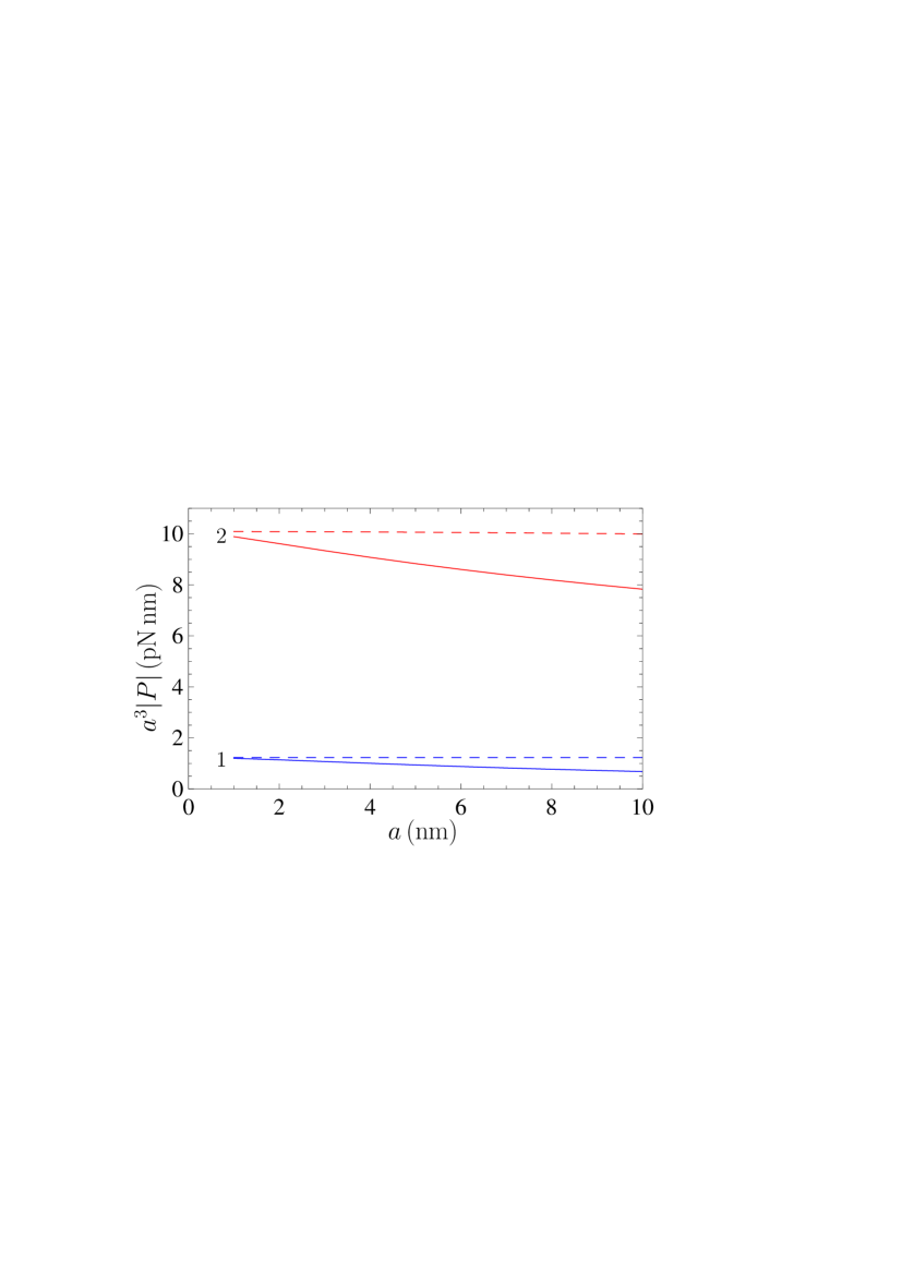
Figure 1: (Color online) The magnitudes of the Casimir pressure between two parallel isotropic plates interacting through a uniaxial anisotropic film (BeO) multiplied by $a^{3}$ are calculated at $T=300\,$K as functions of film thickness using the exact Lifshitz formula (the solid lines) and in the nonrelativistic limit (the dashed lines). The lines 1 and 2 are plotted for the case of SiO₂ and Au plates, respectively.

We substitute Eqs. (22) and (23) in Eq. 13) for the reflection coefficients and calculate the Casimir pressure across a uniaxial anisotropic film at $T=300\,$K by Eq. (12) as a function of the film thickness. The computational results for the magnitude of the Casimir pressure multiplied by the third power of film thickness are presented in Fig. 1 by the solid line 1 for the range of film thicknesses from 1 to 10 nm. In the same figure the dashed line 1 shows the computational results obtained using Eq. (20) for $P_{\rm nr}(a,T)$, i.e., in the nonrelativistic limit. As can be seen in Fig. 1, for a gap filled by the anisotropic material, the nonrelativistic results differ from the exact ones significantly even for very thin films. The relative error of the nonrelativistic Casimir pressure (20)

$$\delta P_{\rm nr}=\frac{|P_{\rm nr}|-|P|}{|P|}$$ (23)

is equal to 2.6%, 8.0%, 30.9%. and 79.8% for film thicknesses of 1, 2, 5, and 10 nm, respectively. For comparison, the same relative error for two SiO₂ plates interacting across a vacuum gap is equal to 0.98%, 3.0%, 12.0%, and 30.5% at the same respective separations. Note that even for a vacuum gap, the application region of the nonrelativistic Lifshitz formula (the van der Waals regime) is restricted to very short separations up to several nanometers. As to the gap, filled by an anisotropic material, the error of the nonrelativistic Casimir pressure becomes too large even for the smallest film thicknesses, and for $a=10\,$nm the nonrelativistic result is already rudely incorrect. Thus, our calculations do not support the statement 18 that the nonretarded limit can be used to calculate the Casimir force between surfaces in uniaxial anisotropic media up to separation distance of $1\,\mu$m.

In Fig. 2(a) we present our computational results over the wide range of film thicknesses from 10 nm to $3\,\mu$m (the solid line). Taking into account that the attractive (negative) Casimir force for large $a$ depends on separation differently than at short separations, here we plot the Casimir pressure multiplied by the fourth power of separation. As can be seen in Fig. 2(a), for film thicknesses larger than approximately $2\,\mu$m the solid line becomes straight, i.e., coincides with the dashed line which describes the large separation (high temperature) classical limit. In this limiting case the Casimir pressure is inverse proportional to $a^{3}$ (see Sec. IV for analytic expressions of the Casimir free energy and pressure across a uniaxial anisotropic film in the classical limit and related discussion). Now we only note that for the vacuum gap between two plates the classical limit is achieved at larger separations of about $6\,\mu$m 5 .

Next, we consider two parallel plates made of Au interacting through the same uniaxial anisotropic film made of BeO. The dielectric permittivity of Au along the imaginary frequency axis is widely discussed in the literature in connection with experiments on measuring the Casimir force (see Refs. 2 ; 5 for a review). The imaginary part of the dielectric permittivity along the real frequency axis is usually obtained by using the tabulated optical data for the complex index of refraction of Au 24 extrapolated down to zero frequency either by the Drude model or by the plasma model. Then, the values of $\varepsilon^{(+1)}=\varepsilon^{(-1)}$ at the imaginary Matsubara frequencies are found by means of the Kramers-Kronig relation. Note that extrapolations using the plasma frequency of Au $\omega_{p}=9.0\,$eV were found to be in excellent agreement with the dielectric permittivities of Au at the imaginary Matsubara frequencies found by means of the weighted Kramers-Kronig relations based solely on the measured optical data 25 . From the standard theoretical point of view, the use of the Drude model extrapolation to low frequencies is considered as preferable. However, the experimental data of many precise experiments on measuring the Casimir interaction between metallic surfaces performed by different experimental groups are consistent with the plasma model extrapolation and exclude the Drude model extrapolation 2 ; 5 ; 26 ; 27 ; 28 ; 29 ; 30 ; 31 ; 32 . The measure of consistency achieves 90% 33 and the measure of exclusion is as high as up to 99.9% 28 . Some doubts were remaining until very recently because in all these experiments, performed at separations below a micrometer, the difference in theoretical predictions using different extrapolations does not exceed a few percent of the measured quantity. Important breakthrough was achieved after the publication of Ref. 34 (see also Ref. 35 ), which proposed the differential experiment where theoretical predictions using the Drude and the plasma model extrapolations differ by a factor of 1000. The recently reported first data sets of this experiment are in agreement with the plasma model extrapolation and exclude the Drude model one 36 .

Taking into account the above discussion, we use in our computations the dielectric permittivity of Au obtained by using the tabulated optical data 24 extrapolated to low frequencies by means of the plasma model 5 . The magnitudes of the Casimir pressure multiplied by $a^{3}$ are computed using Eqs. (12) and (13) and are shown by the solid line 2 in Fig. 1. The dashed line 2 presents the nonrelativistic results for the Casimir pressure between two Au plates across a gap filled by the uniaxial anisotropic material. These results are obtained by using Eqs. (14) and (15). As is seen in Fig. 1, the nonrelativistic results, i.e., the nonretarded van der Waals force, deviate significantly from the exact results even at the shortest separations between the plates. Thus, at $a=1$, 2, 5, and 10 nm the relative error (23) in the nonrelativistic pressure is equal to 2%, 4.9%, 13.9%, and 27.6%. Although these errors are smaller than those in the case of dielectric plates, they demonstrate that even for very thin films the relativistic effects contribute essentially.

In Fig. 2(b) we plot the Casimir pressure between two Au plates across a uniaxial BeO film multiplied by the fourth power of separation over the wide separation region from 10 nm to $3\,\mu$m (the solid line). As is seen from Fig. 2(b), in the region from 500 to 1000 nm the solid line demonstrates nearly constant behavior, i.e., the characteristic for metallic plates dependence of the Casimir pressure $\sim a^{-4}$. At separations above approximately $2.5\,\mu$m the solid line merges with the straight dashed line demonstrating the characteristic behavior of the Casimir pressure at large separations (high temperatures), i.e., the classical limit (see the analytic results for the Casimir free energy and pressure in this case in Sec. IV). Similar to the case of dielectric plates, here the classical limit is achieved at much shorter separations between the plates than for a vacuum gap.

Finally, we briefly discuss the case of dissimilar plates, i.e., one plate made of dielectric (SiO₂) and another one made of metal (Au). It is common knowledge that the 3-layer systems with some relationships between the dielectric permittivities of the layers demonstrate the effect of the Casimir repulsion 4 ; 5 ; 12 ; 13 , which was observed experimentally 37 in the case of an isotropic liquid film sandwiched between two isotropic plates. In our case of two dissimilar plates and a gap filled by an anisotropic material the static dielectric permittivities satisfy the inequalities

$$\varepsilon^{(-1)}(0)<\varepsilon_{xx}^{(0)}(0)<\varepsilon_{zz}^{(0)}(0)<\varepsilon^{(+1)}(0)=\infty$$ (24)

and one should expect the effect of repulsion. This expectation is confirmed by the computational results.

In Fig. 3 we present on the logarithmic scale the values of the Casimir pressure computed by Eqs. (12) and (13) for the film thicknesses from 1 nm to $5\,\mu$m. As is seen from Fig. 3, the Casimir pressure is positive over the entire range of film thicknesses which corresponds to the Casimir repulsion. At separations above approximately $2\,\mu$m the Casimir pressure between two dissimilar plates across a uniaxial anisotropic gap becomes classical, i.e., behaves as $\sim a^{-3}$. This region is shown by the dashed line in Fig. 3. It is discussed in more details in the next section.

IV The classical Casimir effect across a uniaxial anisotropic film

Here, we derive simple analytic expressions for the Casimir free energy and pressure between two isotropic plates separated by a uniaxial dielectric film in the case of large film thicknesses (high temperatures). In this case all terms with $l\geq 1$ in Eqs. (1) and (6) are exponentially small and only the terms with $l=0$ determine the total result 5 . From Eqs. (2)–(4) in the case of two dielectric plates we obtain

$$r_{\rm TM}^{(0,\pm 1)}(0)=\frac{\varepsilon_{0}^{(\pm 1)}-\sqrt{\varepsilon_{xx,0}^{(0)}\varepsilon_{zz,0}^{(0)}}}{\varepsilon_{0}^{(\pm 1)}+\sqrt{\varepsilon_{xx,0}^{(0)}\varepsilon_{zz,0}^{(0)}}}$$

$$r_{\rm TE}^{(0,\pm 1)}(0)=0.$$ (25)

Substituting Eq. (25) in Eqs. (1) and (6) restricted to the term $l=0$, one obtains

$${\cal F}_{\rm cl}(a,T)=\frac{k_{B}T}{4\pi}\int_{0}^{\infty}k_{\bot}dk_{\bot}\ln\left[1-r_{\rm TM}^{(0,+1)}(0)r_{\rm TM}^{(0,-1)}(0)e^{-2ak_{\bot}\sqrt{\varepsilon_{xx,0}^{(0)}}/\sqrt{\varepsilon_{zz,0}^{(0)}}}\right],$$

(26)

$${P}_{\rm cl}(a,T)=-\frac{k_{B}T}{2\pi}\sqrt{\frac{\varepsilon_{xx,0}^{(0)}}{\varepsilon_{zz,0}^{(0)}}}\int_{0}^{\infty}k_{\bot}^{2}dk_{\bot}\left[\frac{e^{2ak_{\bot}\sqrt{\varepsilon_{xx,0}^{(0)}}/\sqrt{\varepsilon_{zz,0}^{(0)}}}}{r_{\rm TM}^{(0,+1)}(0)r_{\rm TM}^{(0,-1)}(0)}-1\right]^{-1}.$$

Now it is convenient to introduce the new variable (16) with $l=0$ and repeat the same calculation as in Eqs. (17)–(19) with the result

$${\cal F}_{\rm cl}(a,T)=-\frac{k_{B}T}{16\pi a^{2}}\frac{\varepsilon_{zz,0}^{(0)}}{\varepsilon_{xx,0}^{(0)}}{\rm Li}_{3}\left[r_{\rm TM}^{(0,+1)}(0)r_{\rm TM}^{(0,-1)}(0)\right],$$

(27)

$${P}_{\rm cl}(a,T)=-\frac{k_{B}T}{8\pi a^{3}}\frac{\varepsilon_{zz,0}^{(0)}}{\varepsilon_{xx,0}^{(0)}}{\rm Li}_{3}\left[r_{\rm TM}^{(0,+1)}(0)r_{\rm TM}^{(0,-1)}(0)\right].$$

As compared to the case of an isotropic material in the gap between plates, here we have the additional factor ${\varepsilon_{zz,0}^{(0)}}/{\varepsilon_{xx,0}^{(0)}}$.

Similar situation holds when one plate is dielectric and another plate is metallic. In this case the TE mode again does not contribute due to $r_{\rm TE}^{(0,-1)}(0)=0$. The TM reflection coefficient for the dielectric film, $r_{\rm TM}^{(0,-1)}(0)$, is again given by Eq. (25). For metallic plate, one has from Eq. (25) $r_{\rm TM}^{(0,+1)}(0)=1$ because $\varepsilon_{0}^{(+1)}=\infty$. As a result, the classical limit for two dissimilar plates, one dielectric and another one metallic, with a uniaxial anisotropic film between them takes the form

$${\cal F}_{\rm cl}(a,T)=-\frac{k_{B}T}{16\pi a^{2}}\frac{\varepsilon_{zz,0}^{(0)}}{\varepsilon_{xx,0}^{(0)}}{\rm Li}_{3}\left[r_{\rm TM}^{(0,-1)}(0)\right],$$

(28)

$${P}_{\rm cl}(a,T)=-\frac{k_{B}T}{8\pi a^{3}}\frac{\varepsilon_{zz,0}^{(0)}}{\varepsilon_{xx,0}^{(0)}}{\rm Li}_{3}\left[r_{\rm TM}^{(0,-1)}(0)\right].$$

Finally we consider the classical limit for two metallic plates with an anisotropic film between them. In this case from Eq. (3) one has $r_{\rm TM}^{(0,\pm 1)}(0)=1$. As to the contribution of the TE mode, it is the same as for two metals separated by the vacuum gap 5 because the quantity $k_{\rm TE}^{(0)}(0,k_{\bot})$ in the second line of Eq. (2) does not depend on $\varepsilon_{xx,0}^{(0)}$. Then, from Eq. (1) with account of Eq. (2) one obtains

$${\cal F}_{\rm cl}(a,T)=-\frac{k_{B}T\zeta(3)}{16\pi a^{2}}\left[\frac{\varepsilon_{zz,0}^{(0)}}{\varepsilon_{xx,0}^{(0)}}+1-4\frac{\delta_{0}}{a}+12\left(\frac{\delta_{0}}{a}\right)^{2}\right],$$ (29)

where $\zeta(z)$ is the Riemann zeta function and $\delta_{0}=\lambda_{p}/(2\pi)=c/\omega_{p}$ is the effective penetration depth of the electromagnetic oscillations into a metal. In a similar way, for the classical Casimir pressure we have

$${P}_{\rm cl}(a,T)=-\frac{k_{B}T\zeta(3)}{8\pi a^{3}}\left[\frac{\varepsilon_{zz,0}^{(0)}}{\varepsilon_{xx,0}^{(0)}}+1-6\frac{\delta_{0}}{a}+24\left(\frac{\delta_{0}}{a}\right)^{2}\right].$$ (30)

As can be seen from Eqs. (29) and (30), there is important qualitative difference between the classical Casimir free energy and pressure in the configuration of two metallic plates separated by the isotropic and anisotropic films. In the case of an isotropic film, the classical Casimir effect does not depend on the material properties of the film. It is the common property for all dielectric films independently of the values of their static dielectric permittivity. By contrast, for uniaxial anisotropic films the classical limit depends on the film material properties in accordance to Eqs. (29) and (30), i.e., through the value of the ratio ${\varepsilon_{zz,0}^{(0)}}/{\varepsilon_{xx,0}^{(0)}}$.

In the end of this section we consider the measure of agreement between the classical Casimir pressures in Eqs. (27), (28) and (30) and the exact values of the Casimir pressure computed numerically in Sec. III. The classical Casimir pressures calculated by the second lines Eqs. (27), (28), and by Eq. (30) are shown by the dashed lines in Figs. 2(a), 3, and 2(b), respectively. The comparison with the respective solid lines shows that for two SiO₂ plates the relative deviation between the magnitudes of the classical and exact Casimir pressures

$$\delta P_{\rm cl}=\frac{|P_{\rm cl}|-|P|}{|P|}$$ (31)

is equal to –6%, –1.97%, –0.56% and –0.15% for film thicknesses equal to 1.5, 2, 2.5, and $3\,\mu$m, respectively. One can conclude that in this case the classical limit is achieved for $a\approx 2\,\mu$m. In a like manner, for two dissimilar Au-SiO₂ plates (Fig. 3) $\delta P_{\rm cl}=5.4$%, 1.4%, 0.33%, and 0.08% at $a=1.5$, 2, 2.5, and $3\,\mu$m, respectively. From Fig. 2(b) (Au-Au plates) one obtains $\delta P_{\rm cl}=-18$%, –6.4%, –1.9%, and –0.55% at the same respective film thicknesses (plate separations). Thus, for Au-SiO₂ and for Au-Au plates interacting across a uniaxial anisotropic film the classical limit is achieved for film thicknesses equal to approximately 2 and $2.5\,\mu$m, respectively.

V Conclusions and discussion

In this paper, we have investigated the thermal Casimir force between two dielectric, metallic and dissimilar (one dielectric and one metallic) plates made of isotropic materials across a dielectric film made of a uniaxial anisotropic crystal. Although the Lifshitz formula for the Casimir free energy and pressure has been generalized for this case in the previous literature, the most of calculations were performed in the nonrelativistic limit, and specific features of the thermal Casimir force with account of retardation effects and in the classical limit were not considered.

According to our results, in this case the role of relativistic effects is much larger than for a vacuum gap, so that the standard theory of the van der Waals force is not applicable even at the shortest separations between the plates. We have obtained simple analytic expressions for the Casimir free energy and pressure in the classical limit, i.e., at large separations (high temperatures). In the case of two metallic plates separated by an isotropic film the classical Casimir free energy and pressure are known to be independent on the film material properties. We demonstrated that this result is not preserved for anisotropic films, where both the Casimir free energy and pressure depend on the ratio of static dielectric permittivities of the film along different coordinate axes. We have also compared the results of numerical computations using the exact Lifshitz formula with the analytical results in the classical limit. It was shown that for two isotropic plates separated by an anisotropic film the classical limit is achieved at much shorter separations than for the plates separated by a vacuum gap.

As was noted in Sec. I, the configuration of a uniaxial film sandwiched between two isotropic plates is of much importance in the investigation of stability of strongly confined (anisotropic) liquid crystals. In this case one can replace the plates with a vacuum and arrive to the free energy of an anisotropic film alone. Very recently, the Lifshitz formula adapted to the case of two-dimensional structures found topical applications in the investigation of the Casimir effect for graphene 38 ; 39 ; 40 ; 41 ; 42 . The most fundamental formalism describing interaction of graphene with the electromagnetic fluctuations is based on the use of the polarization tensor in (2+1)-dimensional space-time 43 ; 44 ; 45 . In its turn, this tensor is equivalent 46 to two (nonlocal) dielectric permittivities, the longitudinal one and the transverse one, in some analogy to the uniaxial crystals considered in this paper.

One can conclude that the Casimir effect for layered structures, where some of the layers are made of anisotropic materials, possesses some unusual properties which can be potentially interesting for both fundamental physics and nanotechnological applications.

         

         

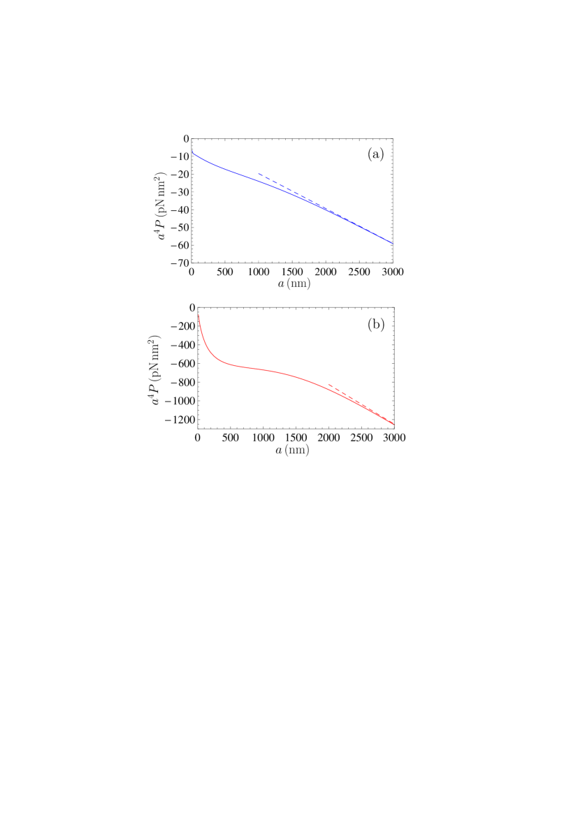
Figure 2: (Color online) The Casimir pressure between two parallel isotropic plates interacting through a uniaxial anisotropic film (BeO) multiplied by $a^{4}$ are calculated at $T=300\,$K as functions of film thickness (the solid lines). The dashed lines show the classical limit. (a) The plates are made of SiO₂. (b) The plates are made of Au.

         

Figure 3: The Casimir pressure between two dissimilar isotropic plates made of SiO₂ and Au interacting through a uniaxial anisotropic film (BeO) is calculated at $T=300\,$K as a function of film thickness (the solid line). The dashed line shows the classical limit.

References

- (1) H. B. G. Casimir, Proc. K. Ned. Akad. Wet. B 51, 793 (1948).
- (2) G. L. Klimchitskaya, U. Mohideen, and V. M. Mostepanenko, Rev. Mod. Phys. 81, 1827 (2009).
- (3) G. L. Klimchitskaya, U. Mohideen, and V. M. Mostepanenko, Int. J. Mod. Phys. B 25, 171 (2011).
- (4) A. W. Rodriguez, F. Capasso, and S. G. Johnson, Nature Photon. 5, 211 (2011).
- (5) M. Bordag, G. L. Klimchitskaya, U. Mohideen, and V. M. Mostepanenko, Advances in the Casimir Effect (Oxford University Press, Oxford, 2015).
- (6) T. Kihara and N. Honda, J. Phys. Soc. Japan 20, 15 (1965).
- (7) V. A. Parsegian and G. H. Weiss, J. Adhes. 3, 259 (1972).
- (8) E. R. Smith and B. W. Ninham, Physica 66, 111 (1973).
- (9) E. M. Lifshitz and L. P. Pitaevskii, Statistical Physics, Part II (Pergamon, Oxford, 1980).
- (10) E. I. Kats, Zh. Eksp. Teor. Fiz. 60, 1172 (1971) [Sov. Phys. JETP 33, 634 (1971)].
- (11) A. Šarlah and S. Žumer, Phys. Rev. E 64, 051606 (2001).
- (12) J. N. Munday, D. Iannuzzi, Yu. Barash, and F. Capasso, Phys. Rev. A 71, 042102 (2005).
- (13) M. B. Romanowsky and F. Capasso, Phys. Rev. A 78, 042110 (2008).
- (14) C.-G. Shao, A.-H. Tong, and J. Luo, Phys. Rev. A 72, 022102 (2005).
- (15) N. P. Zhuck, Int. J. Electronics 75, 141 (1993).
- (16) F. S. S. Rosa, D. A. R. Dalvit, and P. W. Milonni, Phys. Rev. A 78, 032117 (2008).
- (17) E. V. Blagov, G. L. Klimchitskaya, and V. M. Mostepanenko, Phys. Rev. B 71, 235401 (2005).
- (18) P. E. Kornilovitch, J. Phys.: Condens. Matter 25, 035102 (2013).
- (19) M. Boström, C. Persson, and Bo E. Sernelius, Eur. Phys. J. B 86, 43 (2013).
- (20) L. Boinovich and A. Emelyanenko, Adv. Colloid Interface Sci. 165, 60 (2011).
- (21) D. L. Greenaway, G. Harbeke, F. Bassani, and E. Tosatti, Phys. Rev. 178, 1340 (1969).
- (22) L. Hu and S. T. Chui, Phys. Rev. B 66, 085108 (2002).
- (23) L. Bergström, Adv. Colloid Interface Sci. 70, 125 (1997).
- (24) Handbook of Optical Constants of Solids, ed. E. D. Palik (Academic, New York, 1985).
- (25) G. Bimonte, Phys. Rev. A 83, 042109 (2011).
- (26) R. S. Decca, D. López, E. Fischbach, G. L. Klimchitskaya, D. E. Krause, and V. M. Mostepanenko, Ann. Phys. (N. Y.) 318, 37 (2005).
- (27) R. S. Decca, D. López, E. Fischbach, G. L. Klimchitskaya, D. E. Krause, and V. M. Mostepanenko, Phys. Rev. D 75, 077101 (2007).
- (28) R. S. Decca, D. López, E. Fischbach, G. L. Klimchitskaya, D. E. Krause, and V. M. Mostepanenko, Eur. Phys. J. C 51, 963 (2007).
- (29) C.-C. Chang, A. A. Banishev, R. Castillo-Garza, G. L. Klimchitskaya, V. M. Mostepanenko, and U. Mohideen, Phys. Rev. B 85, 165443 (2012).
- (30) A. A. Banishev, C.-C. Chang, G. L. Klimchitskaya, V. M. Mostepanenko, and U. Mohideen, Phys. Rev. B 85, 195422 (2012).
- (31) A. A. Banishev, G. L. Klimchitskaya, V. M. Mostepanenko, and U. Mohideen, Phys. Rev. Lett. 110, 137401 (2013).
- (32) A. A. Banishev, G. L. Klimchitskaya, V. M. Mostepanenko, and U. Mohideen, Phys. Rev. B 88, 155410 (2013).
- (33) V. M. Mostepanenko, arXiv:1411.4548; to be published in J. Phys.: Condens. Matter.
- (34) G. Bimonte, Phys. Rev. Lett. 112, 240401 (2014).
- (35) G. Bimonte, Phys. Rev. Lett. 113, 240405 (2014).
- (36) R. S. Decca, Bulletin Amer. Phys. Soc. 60 (N1) M35.00003 (2015).
- (37) J. N. Munday, F. Capasso, and V. A. Parsegian, Nature 457, 170 (2009).
- (38) G. Gómez-Santos, Phys. Rev. B 80, 245424 (2009).
- (39) D. Drosdoff and L. M. Woods, Phys. Rev. A 84, 062501 (2011).
- (40) M. Bordag, G. L. Klimchitskaya, and V. M. Mostepanenko, Phys. Rev. B 86, 165429 (2012).
- (41) G. L. Klimchitskaya and V. M. Mostepanenko, Phys. Rev. B 87, 075439 (2013).
- (42) Bo E. Sernelius, Phys. Rev. B 90, 155457 (2014).
- (43) M. Bordag, I. V. Fialkovsky, D. M. Gitman, and D. V. Vassilevich, Phys. Rev. B 80, 245406 (2009).
- (44) I. V. Fialkovsky, V. N. Marachevsky, and D. V. Vassilevich, Phys. Rev. B 84, 035446 (2011).
- (45) M. Bordag, G. L. Klimchitskaya, V. M. Mostepanenko, and V. M. Petrov, Phys. Rev. D 91, 045037 (2015).
- (46) G. L. Klimchitskaya, V. M. Mostepanenko, and Bo E. Sernelius, Phys Rev. B 89, 125407 (2014).