A New Equation of State for CCS Pipeline Transport: Calibration of Mixing Rules for Binary Mixtures of CO₂ with N${}_{2},$ O₂ and H₂

Abstract

One of the aspects currently holding back commercial scale deployment of carbon capture and storage (CCS) is an accurate understanding of the thermodynamic behaviour of carbon dioxide and relevant impurities during the pipeline transport stage. In this article we develop a general framework for deriving pressure-explicit EoS for impure CO₂. This flexible framework facilitates ongoing development of custom EoS in response to new data and computational applications. We use our method to generalise a recent EoS for pure CO₂ [Demetriades et al. Proc IMechE Part E, 227 (2013) pp. 117] to binary mixtures with N₂, O₂ and H₂, obtaining model parameters by fitting to experiments made under conditions relevant to CCS-pipeline transport. Our model pertains to pressures up to 16MPa and temperatures between 273K and the critical temperature of pure CO₂. In this region, we achieve close agreement with experimental data. When compared to the GERG EoS, our EoS has a comparable level of agreement with CO₂ -N₂ VLE experiments and demonstrably superior agreement with the O₂ and H₂ VLE data. Finally, we discuss future options to improve the calibration of EoS and to deal with the sparsity of data for some impurities.

1 Introduction and Background

1.1 Carbon capture and storage

Carbon capture and storage is a crucial technology in the international efforts to meet carbon dioxide emission targets [1]. Capturing CO₂ from industrial sources can lead to a $90\%$ reduction in emissions. However, no gas separation process is $100\%$ efficient, and as a result the CO₂ generated from power generation or by industry can contain a number of different impurities, depending on its source. These impurities can, depending on their composition and concentration, greatly influence the physical properties of the fluid compared to pure CO₂. Impurities have important design, safety and cost implications for the compression and transport of CO₂ and its storage location, for example geological sequestration. This research is designed to tackle one of the key technical challenges facing the development of commercially viable CO₂ transport networks: modelling physical behaviour of impure CO₂, under the conditions typically found in carbon capture from power stations, and in high-pressure (liquid phase) and low-pressure (gas phase) pipelines. Accurate modelling of the physical properties of CO₂ mixtures is essential for the design and operation of compression and transport systems for CO₂. In particular the variation of fluid density and phase-behaviour with temperature and pressure is key to many CCS processes. For example, pipeline transport of CO₂ is only viable if the fluid remains in the homogenous phase.

There has been recent work to define the expected operating conditions for CCS pipelines [2, 3]. The most efficient way of transporting CO₂ is in the homogenous phase, at pressures in the vicinity of its critical point. For the transport temperature, the upper temperature will be set by the compressor discharge temperature and the temperature limits of the pipeline coating and the lower temperature will correspond to the winter ground temperature of the surrounding soil[4]. Expected impurity levels are about $\lesssim 4\%$, with N₂ , O₂ and H₂ being key impurities [2, 3, 5, 6]. This range of pressure, temperature and impurity level define pipeline operating conditions and provide a target window for CCS-oriented modelling. However, CCS-relevant models should aspire to model a wider range of conditions, particularly for the impurity level, for the following reasons. Coexistence leads to the formation of a vapour phase that is considerably richer in impurity than the overal mixture. Upset conditions, in which a greater concentration of impurity is accidentally introduced into the CO₂ stream, must be understood and mitigated for. Finally, an effective way to ensure physical robustness of the model is to test for a wider range of impurity conditions.

1.2 CO₂ modelling in CCS

In models of the CCS process, the fluid behaviour of CO₂  mixtures is typically predicted by an equation of state (EoS). EoS vary in their mathematical form, accuracy, region of validity and computational complexity. Because different applications have different requirements there is no single EoS that is ideal for all applications. In particular, there is a balance between mathematical simplicity and accuracy of prediction. To optimise their accuracy, EoS need to be calibrated by fitting their parameters to experimental measurements on CO₂ mixtures. However, new measurements become available very frequently, offering the opportunity to improve the models. Thus, there is an ongoing need to regularly rederive, refine and reparameterise EoS. Currently, the inability to rapidly assimilate ongoing measurements into suitable EoS delays or prevents knowledge gained from experiments from being applied in CCS modelling.

A pressure-explicit EoS is an expression for a fluid’s pressure $P^{*}$, as a function of molar volume $v^{*}$ and temperature $T^{*}$. Usually, the terms in the model that describe the deviation from ideal gas behaviour are empirically postulated. A widely used example is the Peng Robinson equation [7]. Such EoS gives an explicit prediction of the pressure-volume curve for homogeneous fluids and can also predict the coexistence behaviour. For thermodynamic co-existence, the coexisting phases must have matched fugacity for each chemical species, which is equivalent to matching the chemical potential. This translates into a constraint involving the integral of $P^{*}$ over volume, at constant temperature. Thus, the coexistence behaviour can be predicted by numerically searching for two volumes that obey both the EoS and thermodynamic coexistence requirement. Typically, EoS contain empirical parameters that are estimated by fitting the EoS to experimental data for the pure material. These parameter are generalised to mixtures through a set of empirical mixing rules that extend the EoS to multi-component mixtures. These mixing rules also allow calculation of the phase behaviour, through a generalised expression for the fugacity. The pure component parameters and the mixing rules may vary with temperature.

There is an alternative method to formulate EoS, in which the volume and temperature-dependence of the Helmholtz free energy, rather than the pressure, is postulated[8, 9]. Similarly to pressure-explicit EoS, these models contain empirical terms that described the deviation from ideal gas behaviour. The two formulations are, however, mathematically equivalent as integration of a pressure-explicit EoS leads to an expression for the Helmholtz free energy. In this work, we use the pressure-explicit formulation, as measurements of pressure can be directly visualised and so postulating empirical terms for $P^{*}(v^{*})$ is physically more intuitive than for the free energy.

There is considerable uncertainly over which EoS is most appropriate for CCS modelling. Although the Peng-Robinson model is mathematically simple and numerically cheap, it was derived to compute separation of mixtures for the natural gas industry, where CO₂ is a minor additive. Thus, its parameters are optimised to the coexistence behaviour, particularly for the gas phase. Agreement with density measurements for pure CO₂ around the critical pressure, which is key to CCS modelling, is unacceptably poor. Moreover, the mixing rules are not optimised to CCS-relevant mixtures. Variants of the Peng-Robinson model usually suffer the same limitations.

For pure CO₂, the Span-Wagner EoS[8] covers from the triple-point temperature up to very high pressures and temperatures with very high accuracy. Furthermore an EoS by Yokozeki[10] captures solid-liquid coexistence of pure CO₂. Also for pure CO₂, there is a recent composite EoS[11] that combines the Peng-Robinson model for the gas phase and accurate tabulated data for the solid and liquid phases[8, 12, 13]. There have also been studies comparing different pure CO₂ EoS for CCS applications [11, 14]. There are complex and accurate EoS for CO₂ mixtures, including the SAFT[15], PC-SAFT[16], GERG[9] and EOS-CG[17, 18] models. The SAFT, PC-SAFT and EOS-CG models have recently been compared to some CCS-relevant measurements[19, 18]. However, they have not been compared to recently emerged VLE data for CO₂ -H₂ mixtures[20, 6]. Furthermore, the mathematical complexities of these models preclude their use in some CCS applications.

There is clearly considerable scope to derive new EoS, specifically for CO₂ mixtures, retaining the simplicity of Peng-Robinson type equations but with improved quantitative performance for CCS applications. Indeed, a simplified version of the Span-Wagner model for pure CO₂ has been produced[21]. However, the measurements against which a CCS-focussed EoS should be calibrated continually evolve as CCS-oriented projects deliver new data to complement the literature data. Additionally, every user’s requirements differ, depending on the accuracy demanded, the region of interest, and the computational complexity that can be tolerated. Thus, there is no single “silver-bullet” EoS, suitable for all CCS applications and all users. Instead, each application’s requirements can only be met by a bespoke EoS. There is a need for a flexible, general framework to derive and parameterise new EoS in response to emerging measurements and computational applications.

1.3 Aims of this work

In this work we introduce a general and flexible framework for deriving new pressure-explicit EoS. We derive an expression for the mixture fugacity for an arbitrary EoS with arbitrary mixing rules. This allows an EoS to be generalised to mixtures, for any choice of mixing rules, without needing to recompute the fugacity integral. Therefore, our approach allows convenient modification of the form of EoS and mixing rules, in response to new measurement or new physical insights. We demonstrate the flexibility and effectiveness our approach by generalising a recent pressure-explicit EoS for pure CO₂ to mixtures with N₂, O₂ and H₂ and then calibrate this model against data for CCS-relevant mixtures, focussing on pressure-volume behaviour and coexistence. Our approach is readily generalisable to other common CCS impurities, such as argon and methane and can also fit to other thermodynamic variables such as enthalpy and heat capacity.

2 A general expression for the mixture fugacity in pressure-explicit equations of state

In this section we consider a general pressure-explicit EoS and derive results for arbitrary EoS and mixing rules. To compute coexistence we require an expression for the fluid fugacity. For pure fluids this can be obtained by directly integrating the EoS, using eqn (15). Whether this integral can be performed explicitly depends on the expression chosen for the EoS. Furthermore, for the mixture fugacity, one must compute a more complicated integral, involving the mixing rules (eqn (16)). Computing this mixture integral directly is not mathematically convenient for all but the simplest EoS. In this section we show that, provided the pure fluid integral can be performed, then a closed formed expression for the mixture fugacity integral can always be found. Furthermore, we derive a general expression for the mixture fugacity in terms of derivatives of the mixing rule.

We begin with an EoS in the form $P^{\star}=P^{\star}(v^{\star},\boldsymbol{\theta}^{\star},T^{\star})$, where $P^{\star}$ is the pressure in Pa, $v^{\star}$ is the molar volume in mol/m³, $T^{\star}$ is temperature in K and $\boldsymbol{\theta}^{\star}$ is a vector of model parameters. Here, stars denote dimensional quantities. The fugacity co-efficient for the pure fluid, $\ln\phi$, is given by eqn (15) in A. The EoS is generalised to mixtures by allowing the parameter $\boldsymbol{\theta}$ to depend on the fluid composition, $\boldsymbol{x}$, to be specified via a mixing rule. Here $x_{i}$ denotes the mol fraction of species $i$ of the mixture. Leaving the functional forms of $P^{\star}$ and $\boldsymbol{\theta}^{\star}$ unspecified, we show in A that the fugacity coefficient of species $i$ in a mixture is given by

$$\ln\bar{\phi}_{i}(v^{*},\boldsymbol{x})=\ln\phi+\sum_{j=1}^{Np}\frac{\partial F}{\partial\theta^{\star}_{j}}\left(\frac{\partial\theta^{\star}_{j}}{\partial x_{i}}-\sum_{k=1}^{N_{sp}}x_{k}\frac{\partial\theta^{\star}_{j}}{\partial x_{k}}\right),$$ (1)

where $F=\ln\phi-((Z-1)-\ln Z)$. We see that, if the fugacity integral can be performed for the pure fluid, then eqn (1) ensures that the fugacity integral for mixtures can also be written as a closed form expression. Finally, we note that eqn (1) is invariant under a constant scaling of any of the model parameters. This means that the expression is completely unchanged by any non-dimensionalisation that merely scales the model parameters by a constant.

3 A new Equation of State for impure CO₂ 

3.1 Pure CO₂

We begin with a recently proposed EoS for pure CO₂ by Demetriades et al.[22]. The dimensional EoS is

$$P(v^{\star},T^{\star};\boldsymbol{\theta}^{\star})=\frac{RT^{\star}}{v^{\star}+a^{\star}}-\frac{b^{\star 2}}{v^{\star 2}+c^{\star 2}}-\frac{d^{\star 3}}{v^{\star 3}+e^{\star 3}}+\bigg{(}\frac{f^{\star}}{v^{\star}-g^{\star}}\bigg{)}^{6},$$ (2)

where $R$ is the ideal gas contant and $\boldsymbol{\theta}^{\star}=(a^{\star},...,g^{\star})$ is the vector of model parameters. We perform the following non-dimensionalisation, for the physical variables

$$P^{\star}=P_{c}^{\star}P,\;\;\;T^{\star} = T_{c}^{\star}T,\;\;\;v^{\star}=\bigg{(}\frac{RT_{c}}{P_{c}}\bigg{)}v,$$ (3)

and for the model parameters

$$a^{\star}=\bigg{(}\frac{RT^{\star}_{c}}{P^{\star}_{c}}\bigg{)}a,\;\;b^{\star}=\bigg{(}\frac{(RT^{\star}_{c})^{2}}{P^{\star}_{c}}\bigg{)}b,\;\;c^{\star}=\bigg{(}\frac{RT^{\star}_{c}}{P^{\star}_{c}}\bigg{)}^{2}c,\;\;d^{\star}=\bigg{(}\frac{(RT^{\star}_{c})^{3}}{P^{\star 2}_{c}}\bigg{)}d,$$

$$e^{\star}=\bigg{(}\frac{RT^{\star}_{c}}{P^{\star}_{c}}\bigg{)}^{3}e,\;\;f^{\star}=\bigg{(}\frac{RT^{\star}_{c}}{P^{\star 5/6}_{c}}\bigg{)}f,\;\;g^{\star}=\bigg{(}\frac{RT^{\star}_{c}}{P^{\star}_{c}}\bigg{)}g.$$ (4)

Here $P^{\star}_{c}$ and $T_{c}^{\star}$ are the critical pressure and temperature of pure CO₂, respectively. After non-dimensionalisation our EoS becomes

$$P(v,T)=\frac{T}{v+a}-\frac{b^{2}}{v^{2}+c^{2}}-\frac{d^{3}}{v^{3}+e^{3}}+\bigg{(}\frac{f}{v-g}\bigg{)}^{6}.$$ (5)

and the fugacity integral for pure CO₂ (eqn (15)) becomes

$$\ln\phi=\int_{\infty}^{v}\bigg{(}\frac{1}{v^{\prime}}-\frac{P(v^{\prime},T)}{T}\bigg{)}\mathrm{d}v^{\prime}-\ln\bigg{(}\frac{Pv}{T}\bigg{)}+\bigg{(}\frac{Pv}{T}\bigg{)}-1,$$ (6)

which can be evaluated by substituting in eqn (5)

$$\ln\phi(v) = \ln\bigg{(}\frac{v}{a+v}\bigg{)}+\frac{b^{2}}{Tc}\arctan\bigg{(}\frac{v}{c}\bigg{)}$$ (7)

$$+\frac{d^{3}}{3Te^{2}}\ln\bigg{(}\frac{e+v}{\sqrt{e^{2}-ev+v^{2}}}\bigg{)}+\frac{d^{3}}{T\sqrt{3}e^{2}}\arctan\bigg{(}\frac{2v-e}{\sqrt{3}e}\bigg{)}-\frac{f^{6}}{5T(g-v)^{5}}$$

$$-\frac{\pi}{2T}\bigg{(}\frac{b^{2}}{c}+\frac{d^{3}}{\sqrt{3}e^{2}}\bigg{)}-\ln\bigg{(}\frac{P(v)v}{T}\bigg{)}+\bigg{(}\frac{P(v)v}{T}\bigg{)}-1.$$

We repeated the fitting procedure for pure CO₂ from Demetriades et al.[22] to obtain slightly improved agreement with the pure CO₂ data over our previous article. The resulting variation of model parameters with temperature is given by

$$a_{\mathrm{CO_{2}}}(T) = |T-1|^{0.626207}(33.9261|T-1|^{2}-8.10461|T-1|+0.805812)+0.2712941,$$

$$b_{\mathrm{CO_{2}}}(T) = |T-1|^{0.405254}(-13.5708|T-1|^{2}+4.48534|T-1|-0.295229)+0.3326169,$$

$$c_{\mathrm{CO_{2}}}(T) = |T-1|^{0.515789}(-3.77054|T-1|^{2}+1.72673|T-1|{}-0.478733)+0.238762,$$

$$d_{\mathrm{CO_{2}}}(T) = |T-1|^{1.27068}(0.000634507|T-1|^{3}-\text{8.327888244017052E-6}|T-1|^{2}$$

$$-0.0000382867|T-1|+\text{4.661593764290955E-6}){}{}-0.000374407355,$$

$$e_{\mathrm{CO_{2}}}(T) = 0.780746514,$$ (8)

$$f_{\mathrm{CO_{2}}}(T) = |T-1|^{0.192269}(0.210429|T-1|^{2}-0.199813|T-1|{}+0.0528131)+0.0787701,$$

$$g_{\mathrm{CO_{2}}}(T) = |T-1|^{0.198411}(-0.185594|T-1|^{2}+0.0931741|T-1|-0.0510056)+0.074028115.$$

Thus each parameter was fully defined and this completed the model in the case of pure CO₂. We note that the parameter variations given here differ slightly from those proposed in our published work [22]. The model proposed here has a better accuracy than that of our prior version. We now fix these model parameters for the remainder of this article.

3.2 Generalisation to impure CO₂

We generalise our model to impure CO₂ by allowing the model parameters to depend on the impurity concentration, $x_{\mathrm{imp}}$. We opted to impose a linear mixing rule for each of the model parameters in equation (5). For parameter $a$, the mixing rule for a binary mixture of CO₂ and a single impurity (imp) is:

$$a(T)=x_{\mathrm{CO_{2}}}a_{\mathrm{CO_{2}}}(T)+x_{\mathrm{imp}}a_{\mathrm{imp}}(T),$$ (9)

where $a_{\mathrm{CO_{2}}}(T)$is defined in equation (8) for pure CO₂ and $a_{\mathrm{imp}}(T)$ is the analogous quantity for the impurity, which we need to specify. Replacing $a$ in eqn (9) with any of the other model parameters provides the mixing rule for that parameter. We note at this stage that for a binary system

$$x_{\mathrm{imp}}=1-x_{\mathrm{CO_{2}}}.$$ (10)

From here on we use $x$ to denote the impurity fraction.

3.3 Fitting strategy for impurity data

Our fitting strategy for the impurity model is similar to our methodology for pure CO₂ [22], in that we fit model parameters at different temperatures by using simulated annealing, which searches for global minima and has the ability to escape local minima. The correct coexistence behaviour is ensured by imposing a term in the minimisation that penalises differences in the predicted fugacity at the experimentally determined coexistence points (see eqn (12)). This approach requires vapour-liquid equilibrium (VLE) measurements, for both the coexisting mol fractions and molar volumes at each temperature to be fitted.

4 Carbon Dioxide–Nitrogen Binary Mixture

4.1 Data Availability

Temperature (K)	Homogeneous Density	VLE Data
260	[23], [24], [25]
265	[26], [27]
270	[24], [25]	[28]†, [29]†, [30]†, [31]†
273.15	[32], [23], [33]	[32], [34]†, [35, 36],[37]† ,
		[38]†, [39]†, [40]†, [41]†
275	[26], [27], [24], [25], [42]
280	[24], [25]
285	[26], [43], [27], [24], [25]
288.15	[32]	[32], [34]†, [44]†
288.706	[23]
290	[24], [25]
293.3	[45]	[44]†
295	[24], [25]
298.15	[46]	[34]† [37]†
300	[23], [47], [26], [43], [27]
	[24], [25], [48], [42]
301.3		[49]
303.3	[50]	[49]
† means the VLE data in this source do not contain volumes

Table 1: A summary of available data for CO₂ –N₂ mixtures. Experimental data used in our parameter fitting are in boldface.

We begin this section by noting the literature data available to fit the CO₂–N₂ mixture, which is summarised in Table 1. As specified in above, we require VLE data, including coexisting volumes, ideally with homogeneous phase density data all at the same temperature. There are only two relevant temperatures in the literature where this full spread of data exist and, in some cases, the fraction of N₂ used for the homogenous phase measurements is outside the range of relevance to CCS. In order to find the pure N₂ parameter values, we fitted our model to the CO₂ -N₂ mixture data at 273.15K and 288.15K, choosing these temperature as they both had measurements of the coexisting volumes and homogenous phase. A summary of the data used for fitting is as follows. For 273.15K we used VLE data by Muirbrook et al.[35, 36] and homogenous phase data by Arai et al.[32] for $x_{N_{2}}$ in the range $7.1-25.4\%$. For 288.15K we used VLE data by Arai et al.[32] and homogenous phase data by the same authors for $x_{N_{2}}$ in the range $6.0-10.3\%$.

4.2 Fitting the CO₂ –N₂ Binary Model Parameters

We proceeded first by determining the pure N₂ parameters $a_{\mathrm{N_{2}}}$ to $g_{\mathrm{N_{2}}}$ at the available temperature points by a similar series of optimisations as used in the pure CO₂ case. Specifically, we minimised an error function, which in the case of a binary mixture, was comprised of two contributions: from the homogeneous measurements

$$E_{\mathrm{Hom}}=\sum_{i=1}^{N_{h}}\bigg{(}\frac{P(v_{\mathrm{DATA}}^{(i)},T,x_{\mathrm{DATA}}^{(i)})-P_{\mathrm{DATA}}^{(i)}}{P_{\mathrm{DATA}}^{(i)}}\bigg{)}^{2},$$ (11)

where $N_{h}$ is the number of homogeneous measurements at this temperature, $v_{\mathrm{DATA}}^{(i)}$ and $x_{\mathrm{DATA}}^{(i)}$ denote the volume and $N_{2}$ composition, respectively, of the $i$th homogenous data point and $P(v,T,x)$ is the model’s predicted pressure. The second contribution comes from the VLE measurements

$$E_{\mathrm{VLE}} = \sum_{j=1}^{N_{v}}\bigg{[}(P(v_{\mathrm{vap}}^{(j)},T,x^{(j)}_{\mathrm{vap}})-P_{\mathrm{vap}}^{(j)})^{2}{}+(P(v_{\mathrm{liq}}^{(j)},T,x^{(j)}_{\mathrm{liq}})-P_{\mathrm{vap}}^{(j)})^{2}$$ (12)

$$+(\ln\bar{\phi}_{\mathrm{CO_{2}}}(v_{\mathrm{vap}}^{(j)},x^{(j)}_{\mathrm{vap}})-\ln\bar{\phi}_{\mathrm{CO_{2}}}(v_{\mathrm{liq}}^{(j)},x^{(j)}_{\mathrm{liq}})+\ln((1-x^{(j)}_{\mathrm{vap}})/(1-x^{(j)}_{\mathrm{liq}})))^{2}{}$$

$$+(\ln\bar{\phi}_{\mathrm{N_{2}}}(v_{\mathrm{vap}}^{(j)},x^{(j)}_{vap})-\ln\bar{\phi}_{\mathrm{N_{2}}}(v_{\mathrm{liq}}^{(j)},x^{(j)}_{liq})+\ln(x^{(j)}_{\mathrm{vap}}/x^{(j)}_{\mathrm{liq}}))^{2}{}\bigg{]},$$

where $N_{v}$ is the number of VLE measurements at this temperature, $v_{\mathrm{vap/liq}}^{(j)}$ and $x_{\mathrm{vap/liq}}^{(j)}$ denote the coexisting liquid/vapour volume and $N_{2}$ composition, respectively, of the $j$th VLE measurement, $P_{\mathrm{vap}}^{(j)}$ is the $j$th vapour pressure measurement and $\ln\bar{\phi}$ is the model’s predicted fugacity. The two contributions were combined into a total error function

$$E_{\mathrm{Tota}l}=WE_{\mathrm{Hom}}+(1-W)E_{\mathrm{VLE}},$$ (13)

where $W$ is a parameter that determines the weighting of the fitting between homogenous and VLE data. We chose $W=0.1$, to balance fitting between the VLE and homogenous phase data. This generated values for each of the seven pure N₂ parameters at both of the temperature points.

4.3 Variation of Model Parameters with Temperature

$\theta$	$\alpha_{0}$	$\alpha_{1}$
$a_{\mathrm{N_{2}}}$	-2.94804	3.14877
$b_{\mathrm{N_{2}}}$	0.616547	-0.654773
$c_{\mathrm{N_{2}}}$	-4.83602	5.83048
$d_{\mathrm{N_{2}}}$	4.69708	-5.23021
$e_{\mathrm{N_{2}}}$	6.23314	-6.56762
$f_{\mathrm{N_{2}}}$	-11.6889	13.4184
$g_{\mathrm{N_{2}}}$	15.3391	-17.2528

Table 2: Coefficients describing the temperature dependence of the N₂ model parameters in equation (14).

We had determined values for each parameter at each of the two temperatures. To obtain an expression for the temperature dependence of each parameter we converted our parameter values into a linear dependence on temperature,

$$\theta_{\mathrm{N_{2}}}(T)=\alpha_{0}+\alpha_{1}T,$$ (14)

where $\theta$ is a model parameter. The values of $\alpha_{0}$ and $\alpha_{1}$ we obtained for each of the seven N₂ parameters are in table 2

4.4 Performance of the Model for Binary Mixtures of CO₂ and N₂

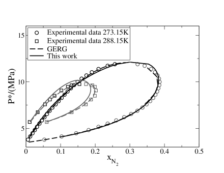
Figure 1: Comparison of experiments and our model for the VLE coexisting mole fraction for CO₂ -N₂ mixtures. Experimental data at 273.15K from Muirbrook et al.[35, 36] and at 288.15K from Arai et al.[32]. Also shown are the results from the GERG EoS [9].

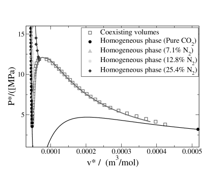
Figure 2: Comparison of experiments and our model for the pressure-volume behaviour of CO₂ -N₂ mixtures at 273.15K in both coexistence and the homogenous phase. Experimental data from Muirbrook et al.[35, 36] (coexistence) and from Arai et al.[32] (homogenous phase).

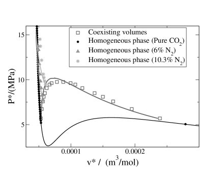
Figure 3: Comparison of experiments and model predictions for the pressure-volume behaviour of CO₂ -N₂ mixtures at 288.15K in both coexistence and the homogenous phase. Experimental data from Arai et al.[32].

With the model thus fully defined for the binary system involving CO₂ and N₂, we were able to assess its performance. We did this by comparing the completed model to the data was used to generate the fitted parameters. We computed the model’s coexistence predictions, at a given temperature, as follows. We began at the pure CO₂ coexistence pressure, where the coexisting volumes are known and the coexisting mol fractions are both $100\%$ CO₂. We then increased the pressure by a small increment and searched for the mol fraction and volume of the liquid and vapour that satisfy the following four coexistence conditions: the liquid phase pressure equals the prescribed pressure; the vapour phase pressure matches the prescribed pressure; the CO₂ fugacity of the liquid matches that of the vapour; and the N₂ fugacity of the liquid matches that of the vapour. We used a numerical non-linear root-finding algorithm to locate the co-existence point. Once the coexistence root was found we increased slightly the pressure and repeated the root finding, using the previous root as an initial guess for the new root. We repeated this process, moving up in small pressure increments, until the critical point was reached.

A comparison between the experiments and our model for the coexisting mol fraction is shown in figure 1. Also shown are the results from the GERG EoS. At both temperatures for both models the agreement is very good. Our model performs similarly to the GERG, except at pressures approaching the critical point for 288.15K. Here, our model fails slightly to capture accurately the approach to the critical point, which is most clearly seen by the rapid convergence of the liquid and vapour mol fraction as the experiments approach the critical pressure, a feature that the GERG captures. For coexisting volumes ( figures 2 and 3) our model performs very well, except for close to the critical point at 288.15K, where our model slightly over-predicts the pressure. Our model captures the mixtures’ pressure-volume data for the homogenous phase (figures 2), except at high pressures at 288.15K where the model’s results are slightly closer to the pure CO₂ behaviour than the experiments. Finally, we also highlight that the best performance of our model occurred for the liquid coexistence properties. This will ensure that the model accurately predicts the liquid saturation line, which is of particular relevance to CCS pipelines as it is the edge of the homogeneous phase region and, ultimately, it defines the minimum safe pipeline operating pressure for a given temperature and overall impurity composition.

Overall, this mixture shows the promise of our methodology. In the areas where our current model fails a little to fully capture the data, namely close to the critical pressure, the flexibility and generality of our approach will enable future work to readily introduce refined mixing rules or terms in the original EoS to obtain further improved agreement. Conversely, our framework will also enable the complexity of the EoS to be reduced for applications that demand a simple EoS but can compromise on the closeness to experiments.

5 Carbon Dioxide–Oxygen Binary Mixture

5.1 Data Availability

Temp.	Homogeneous	VLE Data
	Density
263.15K		[51] †
273.15K		[51] †, [35, 36], [41] †
283.15K		[51] †
302.22K	[50]
† these VLE data do not contain volumes

Table 3: A summary of available data for CO₂ –O₂ binary mixtures. Experimental data used in our parameter fitting are in boldface.

The availability of data for CO₂ –O₂ is more limited than for CO₂ –N₂. A tabulated summary of the relevant available data is given in Table 3. There is a single temperature at which the full array of VLE information was presented, at 273.15K [35, 36]. The highest temperature at which any VLE data is presented is 283.15K, and there is no temperature at which both VLE and density data were given. To enable fitting to a second temperature we developed a volume estimation technique for the co-existing volumes, as detailed in B, to fill-in where experimental measurements were unavailable. A summary of the data used for fitting is as follows. For 273.15K we used VLE data by Muirbrook et al. [35, 36]. For 283.15K we used VLE data from Fredenslund et al.[51], with estimated coexisting volumes. At both temperatures we also used pressure-volume data for pure O₂ from the NIST website [52].

5.2 Fitting the CO₂ –O₂ Binary Model Parameters

To fit the CO₂ –O₂ parameters, we proceeded in exactly the same way as for fitting the impurity parameters in the previous section. We used the error function in eqn (13) and fitted the seven impurity parameters via simulated annealing, treating each temperature separately. We used $W=0.1$, to balance fitting between the VLE and homogenous phase data. To obtain an expression for the temperature dependence of each parameter we converted our parameter values into a linear dependence on temperature (eqn (14)). The coefficients of this linear expression for each of the parameters are listed in table 4.

$\theta$	$\alpha_{0}$	$\alpha_{1}$
$a_{\mathrm{O_{2}}}$	-9.3985	10.4231
$b_{\mathrm{O_{2}}}$	4.62523	-5.15272
$c_{\mathrm{O_{2}}}$	-1.50723	1.9847
$d_{\mathrm{O_{2}}}$	12.838	-14.292
$e_{\mathrm{O_{2}}}$	5.99309	-6.18695
$f_{\mathrm{O_{2}}}$	9.29129	-9.9675
$g_{\mathrm{O_{2}}}$	-7.61445	8.30386

Table 4: Coefficients describing the temperature dependence of the O₂ model parameters in eqn (14).

5.3 Performance of the Full Model for Binary Mixtures of CO₂ and O₂

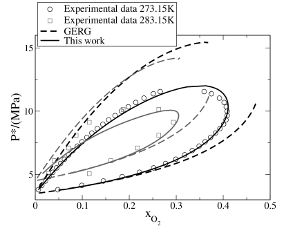
Figure 4: Comparison of experiments and model predictions for the VLE coexisting mole fraction for CO₂ -O₂ mixtures. Experimental data at 273.15K from Muirbrook et al.[35, 36]; and at 283.15K from Fredenslund et al.[51]. Also shown are the results from the GERG EoS [9].

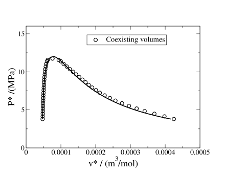
Figure 5: Comparison of experiments and our model for the coexisting volumes for CO₂ -O₂ mixtures at 273.15K. Experimental data from Muirbrook et al.[35, 36].

Similarly, to CO₂ -N₂ mixtures we computed the VLE correlations of the model and compared to the data used for fitting. A comparison between the experiments and our model for the coexisting mol fraction at both temperatures is shown in figure 4. Also shown are the results from the GERG EoS. At 273.15K our model captures well the data, with a very slight discrepancy very close to the critical point. In contrast, the GERG dramatically over-predicts the critical point pressure and has noticeable disagreement with the liquid mol fraction that persists over most of the pressure range. There is a similar picture for the GERG at 283.15K, whereas our model under-predicts somewhat the critical point at this temperature. Overall our model produces consistently better agreement than the GERG. We note the SAFT and PC-SAFT EoS have been compared to these data at 288.15K[19] and both over-predict the critical point pressure to a simular extent to the GERG. Finally the EOS-CG model has also been compared with these experiments[18]. The EoS-CG over-predicts the critical point pressure by $\sim 20\%$ (much less than the GERG and SAFT models) and has better agreement to the liquid mol fraction experiments than our model. Overall our model has superior agreement than the GERG and the SAFT models and comprable agreement to the EOS-CG model.

Figure 5 compares our model with measurements of the coexisting volumes for CO₂ -O₂ mixtures at 273.15K. Agreement is very close throughout.

6 Carbon Dioxide–Hydrogen Binary Mixture

$\theta$	$\alpha_{0}$	$\alpha_{1}$
$a_{\mathrm{H_{2}}}$	-0.919008	0.910607
$b_{\mathrm{H_{2}}}$	-1.00994	0.814616
$c_{\mathrm{H_{2}}}$	-16.5057	18.3776
$d_{\mathrm{H_{2}}}$	0.0204381	-0.0227559
$e_{\mathrm{H_{2}}}$	-16.2801	18.1264
$f_{\mathrm{H_{2}}}$	10.1075	-10.2491
$g_{\mathrm{H_{2}}}$	-4.5342	4.38617

Table 5: Coefficients describing the temperature dependence of the H₂ model parameters in eqn (14).

Coexisting mol fractions for CO₂ -H₂ mixtures under conditions relevant to CCS have recently been measured by Fandiño et al.[20]. We fitted our model to data at 273.15K and 295.65K, to span the temperature range of CCS pipeline operation. As the Fandiño et al. data do not have corresponding coexisting volumes, we required estimated volumes. For 273.15K we were able to validate our volume estimates against the limited CO₂ -H₂ data from [53] at this temperature, enabling us to successfully obtain H₂ parameters. However, the temperature change to 295.65K was sufficiently large that we were unable to successfully fit the Fandiño et al. mol fraction data at this temperature using our volume estimate. Thus we allowed simulated annealing to adjust the parameters of our volume estimation technique in situe, during the fitting, to compensate for the lack of volume data. See B.3 for details. We followed the same fitting procedure as the previous two cases and obtained the temperature dependence of each parameter via eqn (14). The coefficients of this linear temperature rule for each of the parameters are listed in table 5.

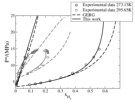
Figure 6: Comparison of experiments and model predictions for the VLE coexisting mole fraction for CO₂ -H₂ mixtures. Experimental data from Fandiño et al.[20]. Also shown are the results from the GERG EoS [9].

A comparison between the experiments and our model for the coexisting mol fraction at both temperatures is shown in figure 6. Also shown are the results from the GERG EoS. Our model captures these data very accurately, with the only disagreement being a slight discrepancy about the critical point for the higher temperature data. In contrast, the GERG EoS substantially over-predicts the critical point pressure at 295.65K, leading to large discrepancies that persist throughout the pressure range. Furthermore, at 273.15K the GERG EoS fails to capture the vapour mol fraction at moderate and higher pressures. Our model produces significantly closer agreement to these data than the GERG EoS. To our knowledge, the SAFT, PC-SAFT and EOS-CG have not been compared to these or comparable data.

7 Discussion

In this article we have developed a general framework for producing pressure-explicit EoS for impure CO₂, aimed at modelling for CCS transport. Under our approach the mixture fugacity integral, required for coexistence calculations, can be computed from the pure fluid fugacity and mixing rules without further integration. This assists ongoing development of EoS in response to new data and computational requirements, as it allows convenient replacement and modification of terms in the EoS and mixing rules.

We used our method to generalise a recent EoS for pure CO₂ to binary mixtures. We used simulated annealing to fit model parameters to experimental data for mixtures with N₂, O₂ and H₂. We captured the coexistence data by imposing a term in the fitting that penalises differences in the predicted fugacity at the experimentally determined coexistence points. Where volumetric measurements were unavailable for coexistence, we developed, tested and exploited a volume estimation method. These estimated volumes allowed us to impose appropriate coexistence behaviour on our model.

For CO₂ -N₂ mixtures, there was comprehensive and high quality literature data across virtually the entire CCS-pipeline window. Such data allowed us to achieve very good fitting with our model to both coexistence and pressure-volume data. For this system our model has comparable agreement to the GERG, but is slightly less accurate. However, for CO₂ -O₂ mixtures our model outperforms the GERG EoS, having more accurate coexisting mol fractions predictions at 273.15K and 288.15K. Our model is also more accurate than the SAFT EoS at 288.15K and has a similar level of agreement to the recent EOS-CG[18]. We also successfully compared to coexisting mol fraction data for CO₂ -H₂ mixtures. Here our model is significantly more accurate than the GERG EoS, particularly at higher temperatures.

A key issue for CCS modelling is the computational complexity of EoS. Some numerical codes use lookup tables of thermophysical properties, whereas other codes use direct, in-situe evaluation of EoS and so require very fast EoS. Our EoS has a moderate number of terms, with inexpensive linear relationships for the mixing rules and the temperature-dependence of the impurity parameters. Furthermore, the pressure expression of our EoS contains only rational functions and so evaluation of this part of the EoS is computationally cheap. The required computational efficiency and whether or not to use lookup tables will depend upon the individual computational task. Ideally, a new EoS would be tailored to the computational and accuracy requirements of the application, a task towards which this work contributes.

A persistent weakness for many EoS is modelling coexistence at pressures and temperatures in the vicinity of the critical point. Although our model is more accurate here than the GERG EoS for CO₂ -O₂ and CO₂ -H₂, it has small discrepancies in this region for all impurities studied herein. This consistent behaviour suggests a systematic difficulty in our current approach, either in locating suitable parameters to describe the vicinity of the critical pressure or in the mathematical terms used in the EoS; and perhaps a difficulty in these factors across all current EoS. We discuss below, improved fitting algorithms that we are currently working on to address this problem. A further possibility to improve these issues is new mixing rules or modified terms in the EoS. We note that our EoS framework will make formulating these modifications straightforward and convenient. However, we leave exploration of these ideas to forthcoming studies.

There are a number of weaknesses to our current approach. Firstly, there is a limit on the number of parameters that can be fitted by simulated annealing to typical experimental data. To control the number of parameters in each search, we fitted individual temperatures separately. Consequently, we could only fit temperatures where VLE mol fractions and volumes were available. Although this was mitigated somewhat by our volume estimation techniques, we still had to exclude some relevant data because the literature experiments were not sufficiently comprehensive at the relevant temperature. However, improved volume estimation or a modified approach to fitting coexistence data may improve the fitting, especially for impurities where mixture data are sparse.

Our approach opens up numerous possibilities to address the above weaknesses. A key issue is the effectiveness of the parameter fitting algorithms. Effective non-linear optimisation is notoriously difficult as parameter-search algorithms often get trapped in deep local minima or struggle to explore effectively a complicated error function (such as eqn (13)). In this work these factors limited the number of parameters we could fit simultaneously. These issues could be addressed by improved fitting algorithms. For example parallel tempering enables search algorithms to escape deep local minima[54] and Riemann manifold, Langevin and Hamiltonian Monte Carlo methods are designed to cope with complicated error surfaces[55]. Such improvements are likely to allow more model parameters to be fitted simultaneously. This will enable the temperature rules for model parameters to be fitted directly, thus meaning that experiments spread across many different temperature can be captured simultaneously. This may improve the EoS’s temperature-dependence around the critical point.

There is also a central role for methods to address missing data or sparse volumetric data. We relied on our volume estimation techniques to stand-in for missing VLE data. A more accurate and physically-based estimate for these volumes could be obtained from molecular simulation[56, 6], provided suitable molecular force fields describing the interaction of CO₂ with relevant impurities can be determined. It is also possible to treat missing VLE data as model parameters and learn these during the fitting process, bypassing the need to explicitly estimate missing coexistence volumes. This introduces many new parameters to the fitting and so is contingent on solving the problem of fitting many parameters simultaneously, either by the techniques mentioned above, or otherwise.

Reasonable solutions to the above issues will enable extensions of this work, targeting features that are useful to CCS applications. These include modelling a wider range of species of impurities, and ternary and higher order mixtures. Another future extension is uncertainty quantifications, which will address uncertainty due to sparsity of data for many impurities and guide the design of future experiments.

8 Conclusions

In this article we have developed a general framework for producing pressure-explicit EoS for impure CO₂, aimed at modelling for CCS transport. This approach allows convenient modification of terms in the EoS and the mixing rules. We used our method to generalise a recent EoS for pure CO₂ to binary mixtures with N₂, O₂ and H₂, introducing 14 new model parameters per impurity. Our model pertains to pressures up to 16MPa and temperatures between 273K and the critical temperature of pure CO₂, $T_{c}$. For CO₂ -N₂ mixtures, our model has comparable agreement to the GERG, but is slightly less accurate. For CO₂ -O₂ mixtures our model outperforms the GERG EoS, for coexistence data at 273.15K and 288.15K. Here, our model is also more accurate than the SAFT EoS at 288.15K and has a similar level of agreement to the recent EOS-CG. We also successfully compared to coexisting mol fraction data for CO₂ -H₂ mixtures. Here our model is significantly more accurate than the GERG EoS, particularly at higher temperatures. We note that it is possible that some pipelines may operate above $T_{c}$, in some regions, which our pure CO₂ model does not currently account for. Fitting this region is more straightforward than the subcritical region due to the lack of coexistence. Furthermore, pipeline failure modelling requires an EoS that is accurate down to the CO₂ triple-point temperature, which is below the range we have explored here. Although our methodology is appropriate to these extensions, we leave them to future work.

Appendix A Mixture Fugacity in Equations of State

We begin with the following fugacity expressions from Orby et al[57]: equation (2.3.9) for the fugacity coefficient of a pure fluid, $\ln\phi$, is

$$\ln\left[\frac{f^{*}_{i}(T^{*},V^{*})}{P^{*}}\right]=\ln\phi=\frac{1}{RT^{*}}\int_{\infty}^{V^{*}}\frac{RT^{*}}{V^{\prime*}}-\frac{P^{*}}{N}\mathrm{d}V^{\prime*}-\ln Z+(Z-1),$$ (15)

where $V^{*}$, $N$ and $Z=P^{*}v^{*}/RT^{*}$ denote the volume, total number of moles and compressibility, respectively; and equation (2.3.1) for the fugacity coefficient of species $i$ in a mixture is

$$\ln\left[\frac{f^{*}_{i}}{P^{*}x_{i}}\right]=\ln\bar{\phi}_{i}=\frac{1}{RT^{*}}\int_{\infty}^{V^{*}}\frac{RT^{*}}{V^{\prime*}}-\left(\frac{\partial P^{*}}{\partial N_{i}}\right)_{T^{*},V^{*},N_{j\neq i}}\mathrm{d}V^{\prime*}-\ln Z,$$ (16)

where $N_{i}$ and $x_{i}$ are the total number of mols and mol fraction, respectively, of species $i$. All variables in dimensional units are notated with stars.

Pressure-explicit EoS are of the form $P^{*}=P(v^{*},\boldsymbol{\theta}^{*}(N_{i}))$, where $v^{*}=\frac{V^{*}}{N}$, so we can use the chain rule to write

$$\left(\frac{\partial P^{*}}{\partial N_{i}}\right)_{T^{*},V^{*},N_{j\neq i}}=-\frac{\partial P^{*}}{\partial V^{*}}\frac{V^{*}}{N_{T}}+\sum_{j=1}^{N_{p}}\frac{\partial P^{*}}{\partial\theta^{*}_{j}}\frac{\partial\theta^{*}_{j}}{\partial N_{i}},$$ (17)

where $N_{p}$ is the number of model parameters. Substituting into equation (16) gives

$$\ln\bar{\phi}_{i}=\left(\frac{1}{RT^{*}}\int_{\infty}^{V^{*}}\frac{RT^{*}}{V^{\prime*}}+\frac{\partial P^{*}}{\partial V^{\prime*}}\frac{V^{\prime*}}{N_{T}}\mathrm{d}V^{\prime*}-\ln Z\right)-\frac{1}{RT^{*}}\sum_{j=1}^{N_{p}}\frac{\partial\theta^{*}_{j}}{\partial N_{i}}\int_{\infty}^{V^{*}}\frac{\partial P^{*}}{\partial\theta^{*}_{j}}\mathrm{d}V^{\prime*}.$$ (18)

Integration by parts shows that the term inside the brackets is equal to $\ln\phi$ (by eqn (15)). Furthermore, defining $F$ to be the integral from eqn (15), i.e. $F=\frac{1}{RT^{*}}\int_{\infty}^{V^{*}}\frac{RT^{*}}{V^{\prime*}}-\frac{P^{*}}{N}\mathrm{d}V^{\prime}=\ln\phi-((Z-1)-\ln Z)$, allows us to write.

$$-N\frac{\partial F}{\partial\theta^{*}_{j}}=\frac{1}{RT^{*}}\int_{\infty}^{V^{*}}\frac{\partial P^{*}}{\partial\theta^{*}_{j}}\mathrm{d}V^{\prime*}.$$ (19)

Substituting (19) into equation (18) gives

$$\ln\bar{\phi}_{i}=\ln\phi+N\sum_{j=1}^{N_{p}}\frac{\partial F}{\partial\theta^{*}_{j}}\frac{\partial\theta^{*}_{j}}{\partial N_{i}}.$$ (20)

The mixing rule will be of the form $\boldsymbol{\theta}^{*}=\boldsymbol{\theta}^{*}(x_{i},\{x_{k\neq i}\})$, where $x_{i}$ is the mol fraction of species $i$ and the $x_{k}$ are the mol fractions of all of the remaining species. Hence, we must now convert the derivative $\frac{\partial\theta^{*}_{j}}{\partial N_{i}}$ in eqn (20) into a derivative with respect to the mol fractions. We have $x_{i}=\frac{N_{i}}{N_{i}+N_{other}}$ where $N_{other}$ is the total number of mols of all species other than $i$. Similarly for $k\neq i$, we have $x_{k}=\frac{N_{k}}{N_{i}+N_{other}}$. Differentiating $\theta^{*}_{j}$ with respect to $N_{i}$ gives

$$\frac{\partial\theta^{*}_{j}}{\partial N_{i}}=\frac{\partial\theta^{*}_{j}}{\partial x_{i}}\frac{\partial x_{i}}{\partial N_{i}}+\sum_{k\neq i}\frac{\partial\theta^{*}_{j}}{\partial x_{k}}\frac{\partial x_{k}}{\partial N_{i}}.$$ (21)

Differentiating the expressions for $x_{i}$ and $x_{k}$ allows us to write

$$N\frac{\partial x_{i}}{\partial N_{i}}=1-x_{i}\;\;\mbox{ and }\;\;N\frac{\partial x_{k}}{\partial N_{i}}=-x_{k}\;\;(\mbox{for }k\neq i).$$ (22)

Substituting equations (21) and (22) into equation (20) gives

$$\ln\bar{\phi}_{i}=\ln\phi+\sum_{j=1}^{Np}\frac{\partial F}{\partial\theta^{*}_{j}}\left(\frac{\partial\theta^{*}_{j}}{\partial x_{i}}-\sum_{k=1}^{N_{sp}}x_{k}\frac{\partial\theta^{*}_{j}}{\partial x_{k}}\right).$$ (23)

We note here that, since the fugacity coefficients are dimensionless, then the mixing rules $\boldsymbol{\theta}^{*}$ are the only dimensional quantities in eqn (23). Furthermore, because of the arrangement of the $\boldsymbol{\theta}^{*}$ terms in (23), the expression is unchanged by any constant scaling of the parameters $\boldsymbol{\theta}^{*}$. Thus we conclude that the form of eqn (23) is unchanged by any non-dimensionalisation that applies a constant scaling to the model parameters.

Appendix B Estimation Molar Volumes for Mixtures

As noted previously, we observed that a lot of literature VLE data lacks measurement of the coexisting volumes. We thus developed from scratch a novel process to estimate both the liquid and vapour volumes in compensation for those data missing in the literature. This was primarily because our method of fitting the parameters required all elements of the thermodynamic description (temperature, pressure, volumes and compositions) to be present. We acknowledge that experimental measurements are clearly preferable to estimated volumes and have only used this technique when measurements are not available.

B.1 Estimating the Coexisting Liquid Volume

We estimated the mixture liquid volume $\tilde{u}_{\mathrm{liq,MIX}}$ by taking a weighted average of the CO₂ volume at the pressure of interest and the pure impurity volume at the same pressure, weighted by the impurity concentration raised to an empirical power $\alpha$. The pure data was available in all cases using standard reference EoS[8, 58, 59, 60] accessed from the NIST website[52]. Our empirical expression for the estimated volume of the coexisting mixture, $\tilde{v}_{\mathrm{liq,MIX}}$, at the required temperature and pressure is,

$$\tilde{v}_{\mathrm{liq,MIX}}=(1-x_{\mathrm{liq}}^{\alpha})v_{\mathrm{CO_{2}}}+x_{\mathrm{liq}}^{\alpha}v_{\mathrm{imp}},$$ (24)

where $x_{\mathrm{liq}}$ is the impurity concentration of the coexisting liquid, $v_{\mathrm{CO_{2}}}$ and $v_{\mathrm{imp}}$ are the pure CO₂ and pure impurity molar volume at the temperature and pressure of interest, and $\alpha$ is an empirically determined constant, included to calibrate this estimation for different mixtures, whose values for different mixtures are given in Table 6.

B.2 Estimating the Coexisting Vapour Volume

The simple weighted average of eqn (24) is ineffective at estimating the coexisting vapour volume, due to the higher impurity fraction and its influence on the CO₂ in the vapour phase. Thus a slightly more complicated expression is required. We used the following expression to estimate the coexisting vapour volume for the vapour,$\tilde{v}_{\mathrm{vap,MIX}}$

$$\tilde{v}_{\mathrm{vap,MIX}}=x_{\mathrm{vap}}^{\beta}v_{\mathrm{CO_{2}}}+v_{\mathrm{imp}}\left(\frac{v_{\mathrm{vap,CO_{2}}}-v_{\mathrm{liq,CO_{2}}}}{v_{\mathrm{imp}}-v_{\mathrm{liq,CO_{2}}}}(1-x_{\mathrm{vap}}^{\beta})+(x_{\mathrm{vap}}-x_{\mathrm{liq}})^{\gamma}\right),$$ (25)

where $x_{\mathrm{vap}}$ is the impurity concentration of the coexisting vapour, $v_{\mathrm{vap,CO_{2}}}$ and $v_{\mathrm{liq,CO_{2}}}$ are the coexisting vapour and liquid volumes for pure CO₂ ,and $\beta$ and $\gamma$ are two further empirically determined constants, given in Table 6. The three empirical exponents depend only on the type of impurity and we determined these by fitting to the coexistence volume measurements used in this work.

Mixture	$\alpha$	$\beta$	$\gamma$
CO2–N2	1.25	0.68	1.01
CO2–O2	1.55	0.47	0.73
CO2–H2	1.51	0.48	1.19

Table 6: A summary of the values for the empirical exponents obtain by fitting to coexisting volume measurements..

When fitting our EoS, we used experimental measurements for the coexisting volumes whenever available and used estimated volumes otherwise. The benefit of this method is that it allows a substitute value for the missing coexisting volumes, which often were not quoted, to be estimated. The technique requires only the pure density data, which was readily available through the NIST website[52] and the coexisting molar fractions, which are widely reported from experiments. A comparison between our estimation technique and co-existing volume measurements used in this work are shown in figures 7, 8 and 9.

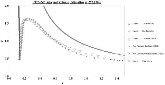
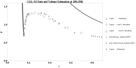
Figure 7: Behaviour of the volume estimation method compared to literature data at 273.15K (top) [35] and 288.15K (bottom) [32] for a CO₂ –N₂ mixture

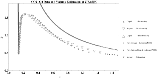
Figure 8: Behaviour of the volume estimation method compared to literature data at 273.15K for a CO₂ –O₂ mixture

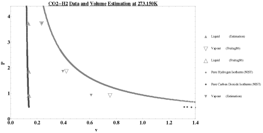
Figure 9: Behaviour of the volume estimation method compared to literature data at 273.15K for a CO₂ –H₂ mixture

B.3 Estimating the CO₂ -H₂ volumes close to the critical point

For 273.15K we were able to validate our volume estimates against the limited CO₂ -H₂ data from ref [53] at this temperature, enabling us to successfully obtain H₂ parameters (see figure 9). However, the temperature step to 295.65K was sufficiently large that we were unable to successfully fit the Fandiño et al. VLE data at this temperature using our volume estimate. Thus we took a slightly more flexible form for the volume estimate

$$\tilde{v}_{\mathrm{vap,MIX}}(P)=(v_{\mathrm{vap,CO_{2}}}-v_{\mathrm{crit}})\left(\frac{P_{\mathrm{crit}}-P}{P_{\mathrm{crit}}-P_{\mathrm{CO_{2}}}}\right)^{\phi}+v_{\mathrm{crit}},$$ (26)

and

$$\tilde{v}_{\mathrm{liq,MIX}}(P)=(v_{\mathrm{liq,CO_{2}}}-v_{\mathrm{crit}})\left(\frac{P_{\mathrm{crit}}-P}{P_{\mathrm{crit}}-P_{\mathrm{CO_{2}}}}\right)^{\phi\left(\frac{v_{\mathrm{crit}}-v_{\mathrm{liq,CO_{2}}}}{v_{\mathrm{vap,CO_{2}}}-v_{\mathrm{crit}}}\right)}+v_{\mathrm{crit}},$$ (27)

where $P_{\mathrm{CO_{2}}}$ is the pure CO₂ coexistence pressure at 295.65K and $P_{\mathrm{crit}}$ is the critical point pressure for CO₂ -H₂ mixtures at 295.65K, which Fandiño et al. evaluated as $P_{\mathrm{crit}}^{*}=14.655$ MPa from their data. The parameters to be fitted are the exponent $\phi$ and the mixture critical volume, $v_{\mathrm{crit}}$. We allowed simulated annealing to adjust the parameters of these two parameters, at the same time as the model parameters, during the fitting at 295.65K. This process gave values of $v_{\mathrm{crit}}=0.320291$ and $\phi=1.02222$.

References

- [1] Boot-Handford, M. E., Abanades, J. C., Anthony, E. J., Blunt, M. J., Brandani, S., Dowell, N. M., Fernández, J. R., Ferrari, M.-C., Gross, R., Hallett, J. P., Haszeldine, R. S., Heptonstall, P., Lyngfelt, A., Makuch, Z., Mangano, E., Porter, R. T. J., Pourkashanian, M., Rochelle, G. T., Shah, N., Yao, J. G., and Fennell, P. S. Carbon capture and storage update. Energy Environ. Sci. 7(1), 130 (2014).
- [2] Seevam, P. N., Race, J. M., and Downie, M. J. Carbon Dioxide Pipelines for Sequestration in the UK: An Engineering Gap Analysis. Journal of Pipeline Engineering 6, pp. 1—14 (2007).
- [3] de Visser, E., Hendriks, C., Barrio, M., lnvik, M. J. M., de Koeijer, G., Liljemark, S., and Gallo, Y. L. Dynamis CO2 Quality Recommendations. International Journal of Greenhouse Gas Control 2, pp. 478—484 (2008). 4th Trondheim Conference on CO2 Capture, Transport and Storage, Trondheim, Norway, OCT 16-17, 2007.
- [4] Mohitpour, M., Seevam, P., Botros, K. K., Rothwell, B., and Ennis, C. Pipeline Transportation of Carbon Dioxide Containing Impurities. ASME Press, New York, NY, USA, (2012).
- [5] Porter, R. T., Fairweather, M., Pourkashaniana, M., and Woolley, R. M. The range and level of impurities in co2 streams from different carbon capture sources. International Journal of Greenhouse Gas Control 36, 161–174 (2015).
- [6] Tenorio, M.-J., Parrot, A. J., Calladine, J., Sanchez-Vicente, Y., Cresswell, A. J., Graham, R. S., Drage, T. C., Poliakoff, M., Ke, J., and George, M. W. The vapour-liquid equilibrium of binary and ternary mixtures of co2, n2 and h2, systems which are of relevance to ccs technology. International Journal of Greenhouse Gas Control (2015).
- [7] Peng, D.-Y. and Robinson, D. B. A New Two–Constant Equation of State. Ind. Eng. Chem. Fundam. 15(1), pp. 59—64 (1976).
- [8] Span, R. and Wagner, W. A New Equation of State for Carbon Dioxide Covering the Fluid Region from the Triple–Point Temperature to 1100 K at Pressures up to 800 MPa. J. Phys. Chem. Ref. Data 25(6), pp. 1509—1596 (1996).
- [9] Kunz, O., Klimeck, R., Wagner, W., and Jaeschke, M. The GERG-2004 wide-range reference equation of state for natural gases. Fortschr.-Ber. VDI, VDI-Verlag, Düsseldorf, (2007).
- [10] Yokozeki, A. Solid–liquid–vapor phases of water and water–carbon dioxide mixtures using a simple analytical equation of state. Fluid Phase Equilibria 222-223, 55–66 (2004).
- [11] Wareing, C. J., Woolley, R. M., Fairweather, M., and Falle, S. A. E. G. A composite equation of state for the modeling of sonic carbon dioxide jets in carbon capture and storage scenarios. Aiche J 59(10), 3928–3942 (2013).
- [12] Trusler, J. P. M. Equation of state for solid phase i of carbon dioxide valid for temperatures up to 800 k and pressures up to 12 gpa. J. Phys. Chem. Ref. Data 40(4), 043105 (2011).
- [13] Jäger, A. and Span, R. Equation of state for solid carbon dioxide based on the gibbs free energy. J. Chem. Eng. Data 57(2), 590–597 (2012).
- [14] Han, W. S. and McPherson, B. Comparison of two different equations of state for application of carbon dioxide sequestration. Advances in Water Resources 31(6), 877–890 (2008).
- [15] Chapman, W. G., Gubbins, K. E., Jackson, G., and Radosz, M. SAFT: Equation–of–State Solution Model for Associating Fluids. Fluid Phase Equilibria 52, pp. 31—38 (1989).
- [16] Gross, J. and Sadowski, G. Perturbed-chain saft: An equation of state based on a perturbation theory for chain molecules. Ind. Eng. Chem. Res. 40(4), 1244–1260 (2001).
- [17] Span, R., Gernert, J., and Jäger, A. Accurate thermodynamic-property models for co2-rich mixtures. Energy Procedia 37, 2914–2922 (2013).
- [18] Gernert, G. J. A New Helmholtz Energy Model For Humid Gases And CCS Mixtures. PhD thesis, Faculty of Mechanical Engineering, University of Bochum, (2013).
- [19] Diamantonis, N. I., Boulougouris, G. C., Mansoor, E., Tsangaris, D. M., and Economou, I. G. Evaluation of cubic, saft, and pc-saft equations of state for the vapor–liquid equilibrium modeling of co 2mixtures with other gases. Ind. Eng. Chem. Res. 52, 3933−3942 (2013).
- [20] Fandiño, O., Trusler, J. M., and Vega-Maza, D. Phase behavior of (co2+h2) and (co2+n2) at temperatures between (218.15 and 303.15)k at pressures up to 15mpa. International Journal of Greenhouse Gas Control 36, 78–92 (2015).
- [21] Span, R. and Wagner, W. Equations of state for technical applications. iii. results for polar fluids. Int J Thermophys 24(1), 111–162 (2003).
- [22] Demetriades, T. A., Drage, T. C., and Graham, R. S. Developing a New Equation of State for Carbon Capture and Storage Pipeline Transport. Proc IMechE Part E: J. Process Mechanical Engineering 227(2), pp. 117—124 (2013).
- [23] Bailey, D. M., Esper, G. J., Holste, J. C., Hall, K. R., Eubank, P. T., Marsh, K. M., and Rogers, W. J. Research Report RR–122: Properties of CO2 Mixtures with N2 and with CH4. Technical report, A Joint Research Report by the Gas Processors Association and the Gas Research Institute, , July (1989).
- [24] Ely, J. F., Magee, J. W., and Haynes, W. M. Research Report RR–110: Thermophysical Properties for Special High CO2 Content Mixtures. Technical report, National Bureau of Standards, Boulder, Colorado, , May (1987).
- [25] Ely, J. F., Haynes, W. M., and Bain, B. C. Isochoric (, , ) Measurements on CO2 and on (0.982CO2 0.018N2) from 250 to 330 K at Pressures to 35 MPa. J. Chem. Thermodynamics 21, pp. 879—894, May (1989).
- [26] Brugge, H. B., Holste, J. C., Hall, K. R., Gammon, B. E., and Marsh, K. N. Densities of Carbon Dioxide Nitrogen from 225 K to 450 K at Pressures up to 70 MPa. J. Chem. Eng. Data 42, pp. 903—907 (1997).
- [27] Duarte-Garza, H., Brugge, H. B., Hwang, C.-A., Eubank, P. T., Holste, J. C., and Hall, K. R. Research Report RR–140: Thermodynamic Properties of CO2 N2 Mixtures. Technical report, A Joint Research Report by the Gas Processors Association and the Gas Research Institute, , June (1995).
- [28] Brown, T. S., Niesen, V. G., Sloan, E. D., and Kidnay, A. J. Vapor–Liquid Equilibria for the Binary Systems of Nitrogen, Carbon Dioxide, and –Butane at Temperatures from 220 to 344 K. Flurd Phase Equilibria 53, pp. 7—14 (1989).
- [29] Brown, T. S., Sloan, E. D., and Kidnay, A. J. Vapor–Liquid Equilibria in the Nitrogen Carbon Dioxide Ethane System. Fluid Phase Equilibria 51, pp. 299—313 (1989).
- [30] Somait, F. A. and Kidnay, A. J. Liquid–Vapor Equilibria at 270.00 K for Systems Containing Nitrogen, Methane, and Carbon Dioxide. Journal of Chemical and Engineering Data 23(4), pp. 301—305 (1978).
- [31] Yucelen, B. and Kidnay, A. J. Vapor–Liquid Equilibria in the Nitrogen Carbon Dioxide Propane System from 240 to 330 K at Pressures to 15 MPa. J. Chem. Eng. Data 44, pp. 926—931 (1999).
- [32] Arai, Y., Kaminishi, G.-I., and Saito, S. The Experiemntal Determination of the ––– Relations for the Carbon Dioxide–Nitrogen and the Carbon Dioxide–Methane Systems. Journal of Chemical Engineering of Japan 4(2), pp. 113—122 (1971).
- [33] Kritschewsky, I. R. and Markov, V. P. The Compressibility of Gas Mixtures. Acta Pysicochimica U. R. S. S. XII(1), pp. 59—66 (1940).
- [34] Kaminishi, G. and Toriumi, T. Vapour–Liquid Phase Equilibria in the CO2–H2, CO2–N2, and CO2–O2 Systems. Kogyo Kagaku Zasshi 69, pp. 175—178 (1966).
- [35] Muribrook, N. K. Experimental and Thermodynamic Study of the High–Pressure Vapor–Liquid Equilibria for the Nitrogen–Oxygen–Carbon Dioxide System. PhD thesis, University of California, (1964).
- [36] Muirbrook, N. K. and Prausnitz, J. M. Multicomponent Vapor–Liquid Equilibria at High Pressures: Part 1. Experimental Study of the Nitrogen–Oxygen–Carbon Dioxide System at 0∘C. A. I. Ch. E. Journal 11(6), pp. 1092—1096, November (1965).
- [37] Yorizane, M., Yoshimura, S., Masuoka, H., Miyano, Y., and Kakimoto, Y. New Procedure for Vapor–Liquid Equilibria. Nitrogen Carbon Dioxide, Methane Freon 22, and Methane Freon 12. J. Chem. Eng. Data 30(2), pp. 174—176 (1985).
- [38] Tsiklis, D. S. Heterogeneous Equilibria in Binary Systems. Russian Journal of Physical Chemistry 20(2), pp. 181—188 (1946).
- [39] Weber, W., Zeck, S., and Knapp, H. Gas Solubilities in Liquid Solvents at High Pressures: Apparatus and Results for Binary and Ternary Systems of N2, CO2, and CH3OH. Fluid Phase Equilibria 18, pp. 253—278 (1984).
- [40] Yorizane, M., Yoshimura, S., and Masuoka, H. Das Dampf–Flü ssigkeits–Gleichgewicht bei hohem Druck Das N2–CO2 und das H2–CO2–System. Chemical Engineering of Japan 34, pp. 1—14 (1970).
- [41] Zenner, G. H. and Dana, L. I. Liquid–Vapor Equilibrium Compositions of Carbon Dioxide–Oxygen–Nitrogen Mixtures. Chemical Engineering Progress Symposium Series 59(44), pp. 36—41 (1963).
- [42] Montagud, M. E. M. Contribution to the Development and Introduction of Renewable Gaseous Fuels Through the Thermodynamic Characterization of Mixtures of their Components by using an Optimized Single Sinker Densimeter with Magnetic Suspension Coupling. PhD thesis, University of Valladolid, (2012).
- [43] Duarte-Garza, H. A., Holste, J. C., Hall, K. R., Marsh, K. N., and Gammon, B. E. Isochoric and Phase Equilibrium Measurements for Carbon Dioxide Nitrogen. J. Chem. Eng. Data 40, pp. 704—711 (1995).
- [44] Xu, N., Dong, J., Wang, Y., and Shi, J. High Pressure Vapor Liquid Equilibria at 293 K for Systems Containing Nitrogen, Methane and Carbon Dioxide. Fluid Phase Equilibria 81, pp. 175—186 (1992).
- [45] Jiang, S., Wang, Y., and Shi, J. Determination of Compressibility Factors and Virial Coefficients for the Systems Containing N2, CO2 and CHClF2 by the Modified Burnett Method. Fluid Phase Equrilibria 57, pp. 105—117, February (1990).
- [46] Haney, R. E. D. and Bliss, H. Compressibilities of Nitrogen–Carbon Dioxide Mixtures. Industrial and Engineering Chemistry 36(11), pp. 985—989, November (1944).
- [47] Brugge, H. B., Hwang, C.-A., Rogers, W. J., Holste, J. C., and Hall, K. R. Experimental Cross Virial Coefficients for Binary Mixtures of Carbon Dioxide with Nitrogen, Methane and Ethane at 300 and 320 K. Physica A 156, pp. 382—416 (1989).
- [48] Esper, G. J., Bailey, O. M., Holste, J. C., and Hall, K. R. Volumetric Behaviour of Near–Equimolar Mixtures for CO2 CH4 and CO2 N2. Fluid Phase Equilibria 49, pp. 35—47 (1989).
- [49] Bian, B., Wang, Y., Shi, J., Zhao, E., and Lu, B. C.-Y. Simultaneous Determination of Vapor–Liquid Equilibrium and Molar Volumes for Coexisting Phases up to the Critical Temperature with a Static Method. Fluid Phase Equilibria 90, pp. 177—187 (1993).
- [50] Mantovani, M., Chiesa, P., Valenti, G., Gatti, M., and Consonni, S. Supercritical Pressure–Density–Temperature Measurements on CO2–N2, CO2–O2 and CO2–Ar Binary Mixtures. J. of Supercritical Fluids 61, pp. 34—43 (2012).
- [51] Fredenslund, A. and Sather, G. A. Gas–Liquid Equilibrium of the Oxygen–Carbon Dioxide System. Journal of Chemical and Engineering Data 15(1), pp. 17—22 (1970).
- [52] The National Institute of Standards and Technology (NIST) Database. The National Institute of Standards and Technology (NIST) Database, (2015).
- [53] Freitag, N. P. and Robinson, D. B. Equilibrium Phase Properties of the Hydrogen–Methans–Carbon Dioxide, Hydrogen–Carbon Dioxide––Pentane and Hydrogen––Pentane Systems. Fluid Phase Equilibria 31, pp. 183—201 (1986).
- [54] Earl, D. J. and Deem, M. W. Parallel tempering: Theory, applications, and new perspectives. Phys. Chem. Chem. Phys. 7(23), 3910 (2005).
- [55] Girolami, M. and Calderhead, B. Riemann manifold Langevin and Hamiltonian Monte Carlo methods. Journal of the Royal Statistical Society: Series B (Statistical Methodology) 73(2), 123–214 (2011).
- [56] Deublein, S., Eckl, B., Stoll, J., Lishchuk, S. V., Guevara-Carrion, G., Glass, C. W., Merker, T., Bernreuther, M., Hasse, H., and Vrabec, J. ms2: A molecular simulation tool for thermodynamic properties. Computer Physics Communications 182(11), 2350–2367 (2011).
- [57] Orbey, H. and Sandler, S. I. Modeling Vapor–Liquid Equilibira: Cubic Equations of State and Their Mixing Rules. Cambridge University Press, (1998).
- [58] Span, R. A reference equation of state for the thermodynamic properties of nitrogen for temperatures from 63.151 to 1000 k and pressures to 2200 mpa. J. Phys. Chem. Ref. Data 29(6), 1361 (2000).
- [59] Leachman, J. W., Jacobsen, R. T., Penoncello, S. G., and Lemmon, E. W. Fundamental equations of state for parahydrogen, normal hydrogen, and orthohydrogen. J. Phys. Chem. Ref. Data 38(3), 721 (2009).
- [60] Schmidt, R. and Wagner, W. A new form of the equation of state for pure substances and its application to oxygen. Fluid Phase Equilibria 19(3), 175–200 (1985).