Identifying Functional Thermodynamics
in
Autonomous Maxwellian Ratchets

Abstract

We introduce a family of Maxwellian Demons for which correlations among information bearing degrees of freedom can be calculated exactly and in compact analytical form. This allows one to precisely determine Demon functional thermodynamic operating regimes, when previous methods either misclassify or simply fail due to approximations they invoke. This reveals that these Demons are more functional than previous candidates. They too behave either as engines, lifting a mass against gravity by extracting energy from a single heat reservoir, or as Landauer erasers, consuming external work to remove information from a sequence of binary symbols by decreasing their individual uncertainty. Going beyond these, our Demon exhibits a new functionality that erases bits not by simply decreasing individual-symbol uncertainty, but by increasing inter-bit correlations (that is, by adding temporal order) while increasing single-symbol uncertainty. In all cases, but especially in the new erasure regime, exactly accounting for informational correlations leads to tight bounds on Demon performance, expressed as a refined Second Law of Thermodynamics that relies on the Kolmogorov-Sinai entropy for dynamical processes and not on changes purely in system configurational entropy, as previously employed. We rigorously derive the refined Second Law under minimal assumptions and so it applies quite broadly—for Demons with and without memory and input sequences that are correlated or not. We note that general Maxwellian Demons readily violate previously proposed, alternative such bounds, while the current bound still holds.

I Introduction

The Second Law of Thermodynamics is only statistically true: while the entropy production in any process is nonnegative on the average, $\langle\Delta S\rangle\geq 0$, if we wait long enough, we shall see individual events for which the entropy production is negative. This is nicely summarized in the recent fluctuation theorem for the probability of entropy production $\Delta S$ [1, 2, 3, 4, 5, 6, 7]:

$$\frac{\Pr(\Delta S)}{\Pr(-\Delta S)}=e^{\Delta S}~{},$$ (1)

implying that negative entropy production events are exponentially rare but not impossible. Negative entropy fluctuations were known much before this modern formulation. In fact, in 1867 J. C. Maxwell used the negative entropy fluctuations in a clever thought experiment, involving an imaginary intelligent being—later called Maxwell’s Demon—that exploits fluctuations to violate the Second Law [8, 9]. The Demon controls a small frictionless trapdoor on a partition inside a box of gas molecules to sort, without any expenditure of work, faster molecules to one side and slower ones to the other. This gives rise to a temperature gradient from an initially uniform system—a violation of the Second Law. Note that the “very observant and neat fingered” Demon’s “intelligence” is necessary; a frictionless trapdoor connected to a spring acting as a valve, for example, cannot achieve the same feat [10].

Maxwell’s Demon posed a fundamental challenge. Either such a Demon could not exist, even in principle, or the Second Law itself needed modification. A glimmer of a resolution came with L. Szilard’s reformulation of Maxwell’s Demon in terms of measurement and feedback-control of a single-molecule engine. Critically, Szilard emphasized hitherto-neglected information-theoretic aspects of the Demon’s operations [11]. Later, through the works of R. Landauer, O. Penrose, and C. Bennett, it was recognized that the Demon’s operation necessarily accumulated information and, for a repeating thermodynamic cycle, erasing this information has an entropic cost that ultimately compensates for the total amount of negative entropy production leveraged by the Demon to extract work [12, 13, 14]. In other words, with intelligence and information-processing capabilities, the Demon merely shifts the entropy burden temporarily to an information reservoir, such as its memory. The cost is repaid whenever the information reservoir becomes full and needs to be reset. This resolution is concisely summarized in Landauer’s Principle [15]: the Demon’s erasure of one bit of information at temperature $T\operatorname{K}$ requires at least $k_{\text{B}}T\ln{2}$ amount of heat dissipation, where $k_{\text{B}}$ is Boltzmann’s constant. (While it does not affect the following directly, it has been known for some time that this principle is only a special case [16].)

Building on this, a modified Second Law was recently proposed that explicitly addresses information processing in a thermodynamic system [17, 18]:

$$\langle\Delta S\rangle+k_{\text{B}}\ln 2\,\Delta\!\operatorname{H}\geq 0~{},$$ (2)

where $\Delta\!\operatorname{H}$ is the change in the information reservoir’s configurational entropy over a thermodynamic cycle. This is the change in the reservoir’s “information-bearing degrees of freedom” as measured using Shannon information $\operatorname{H}$ [19]. These degrees of freedom are coarse-grained states of the reservoir’s microstates—the mesoscopic states that store information needed for the Demon’s thermodynamic control. Importantly for the following, this Second Law assumes explicitly observed Markov system dynamics [17] and quantifies this relevant information only in terms of the distribution of instantaneous system microstates; not, to emphasize, microstate path entropies. In short, while the system’s instantaneous distributions relax and change over time, the information reservoir itself is not allowed to build up and store memory or correlations.

Note that this framework differs from alternative approaches to the thermodynamics of information processing, including: (i) active feedback control by external means, where the thermodynamic account of the Demon’s activities tracks the mutual information between measurement outcomes and system state [20, 21, 22, 23, 24, 25, 26, 27, 28, 29, 30, 31, 32, 33]; (ii) the multipartite framework where, for a set of interacting, stochastic subsystems, the Second Law is expressed via their intrinsic entropy production, correlations among them, and transfer entropy [34, 35, 36, 37]; and (iii) steady-state models that invoke time-scale separation to identify a portion of the overall entropy production as an information current [38, 39]. A unified approach to these perspectives was attempted in Refs. [40, 41, 42].

Recently, Maxwellian Demons have been proposed to explore plausible automated mechanisms that appeal to Eq. (2)’s modified Second Law to do useful work, by deceasing the physical entropy, at the expense of positive change in reservoir Shannon information [43, 44, 39, 45, 46, 47, 48]. Paralleling the modified Second Law’s development and the analyses of the alternatives above, they too neglect correlations in the information-bearing components and, in particular, the mechanisms by which those correlations develop over time. In effect, they account for Demon information-processing by replacing the Shannon information of the components as a whole by the sum of the components’ individual Shannon informations. Since the latter is larger than the former [19], using it can lead to either stricter or looser bounds than the true bound which is derived from differences in total configurational entropies. More troubling, though, bounds that ignore correlations can simply be violated. Finally, and just as critically, they refer to configurational entropies, not the intrinsic dynamical entropy over system trajectories.

This Letter proposes a new Demon for which, for the first time, all correlations among system components can be explicitly accounted. This gives an exact, analytical treatment of the thermodynamically relevant Shannon information change—one that, in addition, accounts for system trajectories not just information in instantaneous state distributions. The result is that, under minimal assumptions, we derive a Second Law that refines Eq. (2) by properly accounting for intrinsic information processing reflected in temporal correlations via the overall dynamic’s Kolmogorov-Sinai entropy [49].

Notably, our Demon is highly functional: Depending on model parameters, it acts both as an engine, by extracting energy from a single reservoir and converting it into work, and as an information eraser, erasing Shannon information at the cost of the external input of work. Moreover, it supports a new and counterintuitive thermodynamic functionality. In contrast with previously reported erasure operations that only decreased single-bit uncertainty, we find a new kind of erasure functionality during which multiple-bit uncertainties are removed by adding correlation (i.e., by adding temporal order), while single-bit uncertainties are actually increased. This new thermodynamic function provocatively suggests why real-world ratchets support memory: The very functioning of memoryful Demons relies on leveraging temporally correlated fluctuations in their environment.

II Information Ratchets

Our model consists of four components, see Fig. 1: (1) an ensemble of bits that acts as an information reservoir; (2) a weight that acts as a reservoir for storing work; (3) a thermal reservoir at temperature $T$; and (4) a finite-state ratchet that mediates interactions between the three reservoirs. The bits interact with the ratchet sequentially and, depending on the incoming bit statistics and Demon parameters, the weight is either raised or lowered against gravity.

As a device that reads and processes a tape of bits, this class of ratchet model has a number of parallels that we mention now, partly to indicate possible future applications. First, one imagines a sophisticated, stateful biomolecule that scans a segment of DNA, say as a DNA polymerase does, leaving behind a modified sequence of nucleotide base-pairs [50] or that acts as an enzyme sequentially catalyzing otherwise unfavorable reactions [51]. Second, there is a rough similarity to a Turing machine sequentially recognizing tape symbols, updating its internal state, and taking an action by modifying the tape cell and moving its read-write head [52]. When the control logic is stochastic, this sometimes is referred to as “Brownian computing” [53, and references therein]. Finally, we are reminded of the deterministic finite-state tape processor of Ref. [54] that, despite its simplicity, indicates how undecidability can be imminent in dynamical processes. Surely there are other intriguing parallels, but these give a sense of a range of applications in which sequential information processing embedded in a thermodynamic system has relevance.

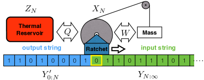
Figure 1: Information ratchet sequentially processing a bit string: At time step $N$, $X_{N}$ is the random variable for the ratchet state and $Z_{N}$ that for the thermal reservoir. $Y_{N:\infty}$ is the block random variable for the input bit string and $Y^{\prime}_{0:N}$ that for the output bit string. The last bit $Y_{N}$ of the input string, highlighted in yellow, interacts with the ratchet. The arrow on the right of the ratchet indicates the direction the ratchet moves along the tape as it sequentially interacts with each input bit in turn.

The bit ensemble is a semi-infinite sequence, broken into incoming and outgoing pieces. The ratchet runs along the sequence, interacting with each bit of the input string step by step. During each interaction at step $N$, the ratchet state $X_{N}$ and interacting bit $Y_{N}$ fluctuate between different internal joint states within $\mathcal{X}_{N}\otimes\mathcal{Y}_{N}$, exchanging energy with the thermal reservoir and work reservoir, and potentially changing $Y_{N}$’s state. At the end of step $N$, after input bit $Y_{N}$ interacts with the ratchet, it becomes the last bit $Y^{\prime}_{N}$ of the output string. By interacting with the ensemble of bits, transducing the input string into the output string, the ratchet can convert thermal energy from the heat reservoir into work energy stored in the weight’s height.

The ratchet interacts with each incoming bit for a time interval $\tau$, starting at the $0$th bit $Y_{0}$ of the input string. After $N$ time intervals, input bit $Y_{N-1}$ finishes interacting with the ratchet and, with the coupling removed, it is effectively “written” to the output string, becoming $Y^{\prime}_{N-1}$. The ratchet then begins interacting with input bit $Y_{N}$. As Fig. 1 illustrates, the state of the overall system is described by the realizations of four random variables: $X_{N}$ for the ratchet state, $Y_{N:\infty}$ for the input string, $Y^{\prime}_{0:N}$ for the output string, and $Z_{N}$ for the thermal reservoir. A random variable like $X_{N}$ realizes elements $x_{N}$ of its physical state space, denoted by alphabet $\mathcal{X}$, with probability $\Pr(X_{N}=x_{N})$. Random variable blocks are denoted $Y_{a:b}=Y_{a}Y_{a+1}\ldots Y_{b-1}$, with the last index being exclusive. In the following, we take binary alphabets for $\mathcal{Y}$ and $\mathcal{Y}^{\prime}$: $y_{N},y^{\prime}_{N}\in\{0,1\}$. The bit ensemble is considered two joint variables $Y^{\prime}_{0:N}=Y^{\prime}_{0}Y^{\prime}_{1}\ldots Y^{\prime}_{N-1}$ and $Y_{N:\infty}=Y_{N}Y_{N+1}\ldots$ rather than one $Y_{0:\infty}$, so that the probability of realizing a word $w\in\{0,1\}^{b-a}$ in the output string is not the same as in the input string. That is, during ratchet operation typically $\Pr(Y_{a:b}=w)\neq\Pr(Y^{\prime}_{a:b}=w)$.

The ratchet steadily transduces the input bit sequence, described by the input word distribution $\Pr(Y_{0:\infty})\equiv\{\Pr(Y_{0:\infty}=w)\}_{w\in\{0,1\}^{\infty}}$—the probability for every semi-infinite input word—into the output string, described by the word distribution $\Pr(Y^{\prime}_{0:\infty})\equiv\{\Pr(Y^{\prime}_{0:\infty}=v)\}_{v\in\{0,1\}^{\ell}}$. We assume that the word distributions we work with are stationary, meaning that $\Pr(Y_{a:a+b})=\Pr(Y_{0:b})$ for all nonnegative integers $a$ and $b$.

A key question in working with a sequence such as $Y_{0:\infty}$ is how random it is. One commonly turns to information theory to provide quantitative measures: the more informative a sequence is, the more random it is. For words at a given length $\ell$ the average amount of information in the $Y_{0:\infty}$ sequence is given by the Shannon block entropy [55]:

$$\operatorname{H}[Y_{0:\ell}]\equiv-\sum_{w\in\{0,1\}^{\ell}}\Pr(Y_{0:\ell}=w)\log_{2}\Pr(Y_{0:\ell}=w).$$ (3)

Due to correlations in typical process sequences, the irreducible randomness per symbol is not the single-symbol entropy $\operatorname{H}[Y_{0}]$. Rather, it is given by the Shannon entropy rate [55]:

$$h_{\mu}\equiv\lim_{\ell\to\infty}\frac{\operatorname{H}[Y_{0:\ell}]}{\ell}~{}.$$ (4)

When applied to a physical system described by a suitable symbolic dynamics, as done here, this quantity is the Kolmogorov-Sinai dynamical entropy of the underlying physical behavior.

Note that these ways of monitoring information are quantitatively quite different. For large $\ell$, $h_{\mu}\ell\ll\operatorname{H}[Y_{0:\ell}]$ and, in particular, anticipating later use, $h_{\mu}\leq\operatorname{H}[Y_{0}]$, typically much less. Equality between the single-symbol entropy and entropy rate is only achieved when the generating process is memoryless. Calculating the single-symbol entropy is typically quite easy, while calculating $h_{\mu}$ for general processes has been known for quite some time to be difficult [56] and it remains a technical challenge [57]. The entropy rates of the output sequence and input sequence are $h_{\mu}^{\prime}=\lim_{\ell\to\infty}\operatorname{H}[Y^{\prime}_{0:\ell}]/\ell$ and $h_{\mu}=\lim_{\ell\to\infty}\operatorname{H}[Y_{0:\ell}]/\ell$, respectively.

The informational properties of the input and output word distributions set bounds on energy flows in the system. Appendix A establishes one of our main results: The average work done by the ratchet is bounded above by the difference in Kolmogorov-Sinai entropy of the input and output processes :

$$\langle W\rangle \leq k_{\text{B}}T\ln 2\,(h_{\mu}^{\prime}-h_{\mu})$$

$$=k_{\text{B}}T\ln 2\,\Delta h_{\mu}~{}.$$ (5)

In light of the preceding remarks on the basic difference between $\operatorname{H}[Y_{0}]$ and $h_{\mu}$, we can now consider more directly the differences between Eqs. (2) and (5). Most importantly, the $\Delta\!\operatorname{H}$ in the former refers to the instantaneous configurational entropy $\operatorname{H}$ before and after a thermodynamic transformation. In the ratchet’s steady state operation, $\Delta\!\operatorname{H}$ vanishes since the configuration distribution is time invariant, even when the overall system’s information production is positive. The entropies $h_{\mu}^{\prime}$ and $h_{\mu}$ in Eq. (5), in contrast, are dynamical: rates of active information generation in the input and output giving, in addition, the correct minimum rates since they take all temporal correlations into account. Together they bound the overall system’s information production in steady state away from zero. In short, though often conflated, configurational entropy and dynamical entropy capture two very different kinds of information and they, per force, are associated with different physical properties supporting different kinds of information processing. They are comparable only in special cases.

For example, if one puts aside this basic difference to facilitate comparison and considers the Shannon entropy change $\Delta\!\operatorname{H}$ in the joint state space of all bits, the two equations are analogous in the current setup. However, often enough, a weaker version of Eq. (2) is considered in the discussions on Maxwell’s Demon [43, 44, 45, 41, 59] and information reservoirs [18], wherein the statistical correlations between the bits are neglected, and one simply interprets $\Delta\operatorname{H}$ to be the change in the marginal Shannon entropies $\operatorname{H}[Y_{0}]$ of the individual bits. This implies the following relation in the current context:

$$\langle W\rangle\leq k_{\text{B}}\ln 2\,\Delta\!\operatorname{H}[Y_{0}]~{},$$ (6)

where $\Delta\operatorname{H}[Y_{0}]=\operatorname{H}[Y_{0}^{\prime}]-\operatorname{H}[Y_{0}]$. While Eq. (6) is valid for the studies in Refs. [43, 44, 45, 41, 18, 59], it cannot be taken as a fundamental law, because it can be violated [60]. In comparison, Eq. (5) is always valid and can even provide a stronger bound.

As an example, consider the case where the ratchet has memory and, for simplicity of exposition, is driven by an uncorrelated input process, meaning the input process entropy rate is the same as the single-symbol entropy: $h_{\mu}=\operatorname{H}[Y_{0}]$. However, the ratchet’s memory can create correlations in the output bit string, so:

$$\Delta h_{\mu} =h_{\mu}^{\prime}-\operatorname{H}[Y_{0}]$$

$$\leq\operatorname{H}[Y^{\prime}_{0}]-\operatorname{H}[Y_{0}]$$

$$=\Delta\!\operatorname{H}[Y_{0}]~{}.$$ (7)

In this case, Eq. (5) is a tighter bound on the work done by the ratchet—a bound that explicitly accounts for correlations within the output bit string the ratchet generates during its operation. For example, for the combination $\{p=0.5,q=0.1,b=0.9\}$, two bits in the outgoing string are correlated even when they are separated by $13$ steps. Previously, the effect of these correlations has not been calculated, but they have important consequences. Due to correlations, it is possible to have an increase in the single-symbol entropy difference $\Delta H[Y_{0}]$ but a decrease in the Kolmogorov-Sinai entropy rate $\Delta h_{\mu}$. In this situation, it is erroneous to assume that there is an increase in the information content in the bits. There is, in fact, a decrease in information because of the correlations; cf. Sec. V.

Note that a somewhat different situation was considered in Ref. [59], a memoryless channel (ratchet) driven by a correlated process. In this special case—ratchets unable to leverage or create temporal correlations—either Eq. (6) or Eq. (5) can be a tighter quantitative bound on work. When a memoryless ratchet is driven by uncorrelated input, though, the bounds are equivalent. Critically, for memoryful ratchets driven by correlated input Eq. (6) can be violated. In all settings, Eq. (5) holds.

While we defer it’s development to a sequel, Eq. (5) also has implications for ratchet functioning when the input bits are correlated as well. Specifically, correlations in the input bits can be leveraged by the ratchet to do additional work—work that cannot be accounted for if one only considers single-symbol configurational entropy of the input bits [61].

III Energetics and Dynamics

To predict how the ratchet interacts with the bit string and weight, we need to specify the string and ratchet energies. When not interacting with the ratchet the energies, $E_{0}$ and $E_{1}$, of both bit states, $Y=0$ and $Y=1$, are taken to be zero for symmetry and simplicity: $E_{0}=E_{1}=0$. For simplicity, too, we say the ratchet mechanism has just two internal states $A$ and $B$. When the ratchet is not interacting with bits, the two states can have different energies. We take $E_{A}=0$ and $E_{B}=-\alpha k_{\text{B}}T$, without loss of generality. Since the bits interact with the ratchet one at a time, we only need to specify the interaction energy of the ratchet and an individual bit. The interaction energy is zero if the bit is in the state $Y=0$, regardless of the ratchet state, and it is $-\beta k_{\text{B}}T$ (or $+\beta k_{\text{B}}T$) if the bit is in state $Y=1$ and the ratchet is in state $A$ (or $B$). See Fig. 2 for a graphical depiction of the energy scheme under “Ratchet $\otimes$ Bit”.

The scheme is further modified by the interaction of the weight with the ratchet and bit string. We attach the weight to the ratchet-bit system such that when the latter transitions from the $B\otimes 0$ state to the $A\otimes 1$ state it lifts the weight, doing a constant amount $wk_{\text{B}}T$ of work. As a result, the energy of the composite system—Demon, interacting bit, and weight—increases by $wk_{\text{B}}T$ whenever the transition $B\otimes 0\rightarrow A\otimes 1$ takes place, the required energy being extracted from the heat reservoir $Z_{N}$. The rightmost part of Fig. 2 indicates this by raising the energy level of $A\otimes 1$ by $wk_{\text{B}}T$ compared to its previous value. Since the transitions between $A\otimes 1$ and $B\otimes 1$ do not involve the weight, their relative energy difference remains unaffected. An increase in the energy of $A\otimes 1$ by $wk_{\text{B}}T$ therefore implies the same increase in the energy of $B\otimes 1$. Again, see Fig. 2 for the energy scheme under “Ratchet $\otimes$ Bit $\otimes$ Weight”.

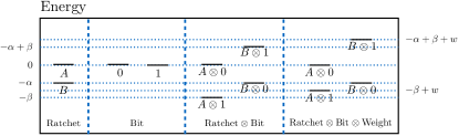
Figure 2: Energy levels of the Demon states, interacting bits, their joint system, and their joint system with a weight in units of $[k_{\text{B}}T]$.

The time evolution over the joint state space of the ratchet, last bit of the input string, and weight is governed by a Markov dynamic, specified by state-transition matrix $M$. If, at the beginning of the $N$th interaction interval at time $t=\tau(N-1)+0^{+}$, the ratchet is in state $X_{N}=x_{N}$ and the input bit is in state $Y_{N}=y_{N}$, then let $M_{x_{N}\otimes y_{N}\rightarrow x_{N+1}\otimes y^{\prime}_{N}}$ be the probability $\Pr(x_{N+1},y^{\prime}_{N}|x_{N},y_{N})$ that the ratchet is in state $X_{N}=x_{N+1}$ and the bit is in state $Y_{N}=y^{\prime}_{N}$ at the end of the interaction interval $t=\tau(N-1)+\tau^{-}$. $X_{N}$ and $Y_{N}$ at the end of the $N$th interaction interval become $X_{N+1}$ and $Y^{\prime}_{N}$ respectively at the beginning of the $N+1$th interaction interval. Since we assume the system is thermalized with a bath at temperature $T$, the ratchet dynamics obey detailed balance. And so, transition rates are governed by the energy differences between joint states:

$$\frac{M_{x_{N}\otimes y_{N}\rightarrow x_{N+1}\otimes y^{\prime}_{N}}}{M_{x_{N+1}\otimes y^{\prime}_{N}\rightarrow x_{N}\otimes y_{N}}}=e^{(E_{x_{N+1}\otimes y^{\prime}_{N}}-E_{x_{N}\otimes y_{N}})/k_{\text{B}}T}~{}.$$ (8)

There is substantial flexibility in constructing a detailed-balanced Markov dynamic for the ratchet, interaction bit, and weight. Consistent with our theme of simplicity, we choose one that has only six allowed transitions: $A\otimes 0\leftrightarrow B\otimes 0$, $A\otimes 1\leftrightarrow B\otimes 1$, and $A\otimes 1\leftrightarrow B\otimes 0$. Such a model is convenient to consider, since it can be described by just two transition probabilities $0\leq p\leq 1$ and $0\leq q\leq 1$, as shown in Fig. 3.

Figure 3: The Markovian, detailed-balance dynamic over the joint states of the ratchet and interacting bit.

The Markov transition matrix for this system is given by:

$$M=\left[\begin{array}[]{cccc}0&1-p&0&0\\ 1&0&q&0\\ 0&p&0&1\\ 0&0&1-q&0\end{array}\right].$$ (13)

This allows allows us to calculate the state distribution $\mathbf{p}((N-1)\tau+\tau^{-})$ at the end of the $N$th interaction interval from the state distribution $\mathbf{p}((N-1)\tau+0^{+})$ at the interval’s beginning via:

$$\mathbf{p}((N-1)\tau+\tau^{-})=M\mathbf{p}((N-1)\tau+0^{+})~{},$$ (14)

where the probability vector is indexed $\mathbf{p}=(\Pr(A\otimes 0),\Pr(B\otimes 0),\Pr(A\otimes 1),\Pr(B\otimes 1))^{\top}$. To satisfy detailed balance, we find that $\alpha$, $\beta$, and $w$ should be:

$$\alpha =-\ln(1-p)~{},$$ (15)

$$\beta =-\frac{1}{2}\ln\left[(1-p)(1-q)\right]~{},~{}\text{and}$$ (16)

$$w =\ln\left(\frac{q\sqrt{1-p}}{p\sqrt{1-q}}\right)~{}.$$ (17)

(Appendix B details the relationships between the transitions probabilities and energy levels.)

This simple model is particularly useful since, as we show shortly, it captures the full range of thermodynamic functionality familiar from previous models and, more importantly, it makes it possible to exactly calculate informational properties of the output string analytically.

Now that we know how the ratchet interacts with the bit string and weight, we need to characterize the input string to predict the energy flow through the ratchet. As in the ratchet models of Refs. [43, 47], we consider an input generated by a biased coin—$\Pr(Y_{N}=0)=b$ at each $N$—which has no correlations between successive bits. For this input, the steady state distributions at the beginning and end of the interaction interval $\tau$ are:

$$\mathbf{p}^{\text{s}}(0^{+}) =\frac{1}{2}\left[\begin{array}[]{c}b\\ b\\ 1-b\\ 1-b\end{array}\right]~{}\text{and}$$ (22)

$$\mathbf{p}^{\text{s}}(\tau^{-}) =\frac{1}{2}\left[\begin{array}[]{c}b(1-p)\\ b+q-bq\\ bp+1-b\\ (1-b)(1-q)\end{array}\right]~{}.$$ (27)

These distributions are needed to calculate the work done by the ratchet.

To calculate net extracted work by the ratchet we need to consider three work-exchange steps for each interaction interval: (1) when the ratchet gets attached to a new bit, to account for their interaction energy; (2) when the joint transitions $B\otimes 0\leftrightarrow A\otimes 1$ take place, to account for the raising or lowering of the weight; and (3) when the ratchet detaches itself from the old bit, again, to account for their nonzero interaction energy. We refer to these incremental works as $W_{1}$, $W_{2}$, and $W_{3}$, respectively.

Consider the work $W_{1}$. If the new bit is in state $0$, from Fig. 2 we see that there is no change in the energy of the joint system of the ratchet and the bit. However, if the new bit is $1$ and the initial state of the ratchet is $A$, energy of the ratchet-bit joint system decreases from 0 to $-\beta$. The corresponding energy is gained as work by the mechanism that makes the ratchet move past the tape of bits. Similarly, if the new bit is $1$ and the initial state of the ratchet is $B$, there is an increase in the joint state energy by $\beta$; this amount of energy is now taken away from the driving mechanism of the ratchet. In the steady state, the average work gain $\langle W_{1}\rangle$ is then obtained from the average decrease in energy of the joint (ratchet-bit) system:

$$\langle W_{1}\rangle =-\sum_{\begin{subarray}{c}x\in\{A,B\}\\ y\in\{0,1\}\end{subarray}}p_{x\otimes y}^{\text{s}}(0^{+})\left(E_{x\otimes y}-E_{x}-E_{y}\right)$$

$$=0~{},$$ (28)

where we used the probabilities in Eq. (27) and Fig. 2’s energies.

By a similar argument, the average work $\langle W_{3}\rangle$ is equal to the average decrease in the energy of the joint system on the departure of the ratchet, given by:

$$\langle W_{3}\rangle=-\frac{k_{\text{B}}T}{2}\beta[q+b(p-q)]~{}.$$ (29)

Note that the cost of moving the Demon on the bit string (or moving the string past a stationary Demon) is accounted for in works $W_{1}$ and $W_{3}$.

Work $W_{2}$ is associated with raising and lowering of the weight depicted in Fig. 1. Since transitions $B\otimes 0\rightarrow A\otimes 1$ raise the weight to give work $k_{\text{B}}Tw$ and reverse transitions $B\otimes 0\leftarrow A\otimes 1$ lower the weight consuming equal amount of work, the average work gain $\langle W_{2}\rangle$ must be $k_{\text{B}}Tw$ times the net probability transition along the former direction, which is $[T_{B\otimes 0\to A\otimes 1}p^{\text{s}}_{B\otimes 0}(0^{+})-T{{}_{A\otimes 1\to A\otimes 1}}p^{\text{s}}_{A\otimes 1}(0^{+})]$. This leads to the following expression:

$$\langle W_{2}\rangle=\frac{k_{\text{B}}Tw}{2}[-q+b(p+q)]~{},$$ (30)

where we used the probabilities in Eq. (27).

The total work supplied by the ratchet and a bit is their sum:

$$\langle W\rangle =\langle W_{1}\rangle+\langle W_{2}\rangle+\langle W_{3}\rangle$$ (31)

$$=\frac{k_{\text{B}}T}{2}[(pb-q+qb)\ln{\left(\frac{q}{p}\right)}$$

$$\quad\quad+(1-b)q\ln(1-q)+pb\ln(1-p)]~{}.$$

Note that we considered the total amount amount of work that can be gained by the system, not just that obtained by raising the weight. Why? As we shall see in Sec. V, the former is the thermodynamically more relevant quantity. A similar energetic scheme that incorporates the effects of interaction has also been discussed in Ref. [48].

In this way, we exactly calculated the work term in Eq. (5). We still need to calculate the entropy rate of the output and input strings to validate the proposed Second Law. For this, we introduce an information-theoretic formalism to monitor processing of the bit strings by the ratchet.

IV Information

To analytically calculate the input and output entropy rates, we consider how the strings are generated. A natural way to incorporate temporal correlations in the input string is to model its generator by a finite-state hidden Markov model (HMM), since HMMs are strictly more powerful than Markov chains in the sense that finite-state HMMs can generate all processes produced by Markov chains, but the reverse is not true. For example, there are processes generated by finite HMMs that cannot be by any finite-state Markov chain. In short, HMMs give a compact representations for a wider range of memoryful processes.

Consider possible input strings to the ratchet. With or without correlations between bits, they can be described by an HMM generator with a finite set of, say, $K$ states and a set of two symbol-labeled transition matrices $T^{(0)}$ and $T^{(1)}$, where:

$$T^{(y_{N})}_{s_{N}\to s_{N+1}}=\Pr(Y_{N}=y_{N},S_{N+1}=s_{N+1}|S_{N}=s_{N})$$ (32)

is the probability of outputting $y_{N}$ for the $N$th bit of the input string and transitioning to internal state $s_{N+1}$ given that the HMM was in state $s_{N}$.

When it comes to the output string, in contrast, we have no choice. We are forced to use HMMs. Since the current input bit state $Y_{N}$ and ratchet state $X_{N}$ are not explicitly captured in the current output bit state $Y^{\prime}_{N}$, $Y_{N}$ and $X_{N}$ are hidden variables. As we noted before, calculating HMM entropy rates is a known challenging problem [56, 57]. Much of the difficulty stems from the fact that in HMM-generated processes the effects of internal states are only indirectly observed and, even then, appear only over long output sequences.

We can circumvent this difficulty by using unifilar HMMs, in which the current state and generated symbol uniquely determine the next state. This is a key technical contribution here since for unifilar HMMs the entropy rate is exactly calculable, as we now explain. Unifilar HMMs internal states are a causal partitioning of the past, meaning that every past $w$ maps to a particular state through some function $f$ and so:

$$\Pr(Y_{N}=y_{N}|Y_{0:N}=w)=\Pr(Y_{N}=y_{N}|S_{N}=f(w))~{}.$$ (33)

As a consequence, the entropy rate $h_{\mu}$ in its block-entropy form (Eq. (4)) can be re-expressed in terms of the transition matrices. First, recall the alternative, equivalent form for entropy rate: $h_{\mu}=\lim_{N\rightarrow\infty}\operatorname{H}[Y_{N}|Y_{0:N}]$. Second, since $S_{N}$ captures all the dependence of $Y_{N}$ on the past, $h_{\mu}=\lim_{N\rightarrow\infty}\operatorname{H}[Y_{N}|S_{N}]$. This finally leads to a closed-form for the entropy rate [55]:

$$h_{\mu} =\lim_{N\rightarrow\infty}\operatorname{H}[Y_{N}|S_{N}]$$

$$=-\sum_{y_{N},s_{N},s_{N+1}}\pi_{s_{N}}T^{(y_{N})}_{s_{N}\rightarrow s_{N+1}}\log_{2}T^{(y_{N})}_{s_{N}\rightarrow s_{N+1}}~{},$$ (34)

where $\pi$ is the stationary distribution over the unifilar HMM’s states.

Figure 4: Biased coin input string as a unifilar hidden Markov model with bias $\Pr(Y=0)=b$.

Let’s now put these observations to work. Here, we assume the ratchet’s input string was generated by a memoryless biased coin. Figure 4 shows its (minimal-size) unifilar HMM. The single internal state $C$ implies that the process is memoryless and the bits are uncorrelated. The HMM’s symbol-labeled ($1\times 1$) transition matrices are $T^{(0)}=\left[b\right]$ and $T^{(1)}=\left[1-b\right]$. The transition from state $C$ to itself labeled $0:b$ means that if the system is in state $C$, then it transitions to state $C$ and outputs $Y=0$ with probability $b$. Since this model is unifilar, we can calculate the input-string entropy rate from Eq. (34) and see that it is the single-symbol entropy of bias $b$:

$$h_{\mu} =\operatorname{H}(b)$$

$$\equiv-b\log_{2}b-(1-b)\log_{2}(1-b)~{},$$ (35)

where $\operatorname{H}(b)$ is the (base $2$) binary entropy function [19].

The more challenging part of our overall analysis is to determine the entropy rate of the output string. Even if the input is uncorrelated, it’s possible that the ratchet creates temporal correlations in the output string. (Indeed, these correlations reflect the ratchet’s operation and so its thermodynamic behavior, as we shall see below.) To calculate the effect of these correlations, we need a generating unifilar HMM for the output process—a process produced by the ratchet being driven by the input.

When discussing the ratchet energetics, there was a Markov dynamic $M$ over the ratchet-bit joint state space. Here, it is now controlled by bits from the input string and writes the result of the thermal interaction with the ratchet to the output string. In this way, $M$ becomes an input-output machine or transducer [62]. In fact, this transducer is a communication channel in the sense of Shannon [63] that communicates the input bit sequence to the output bit sequence. However, it is a channel with memory. Its internal states correspond to the ratchet’s states. To work with $M$, we rewrite it componentwise as:

$$M^{(y^{\prime}_{N}|y_{N})}_{x_{N}\rightarrow x_{N+1}}=M_{x_{N}\otimes y_{N}\rightarrow x_{N+1}\otimes y^{\prime}_{N}}$$ (36)

to evoke its re-tooled operation. The probability of generating bit $y^{\prime}_{N}$ and transitioning to ratchet state $x_{N+1}$, given that the input bit is $y_{N}$ and the ratchet is in state $x_{N}$, is:

$$M^{(y^{\prime}_{N}|y_{N})}_{x_{N}\rightarrow x_{N+1}}=$$ (37)

$$\quad\quad\Pr(Y^{\prime}_{N}=y^{\prime}_{N},X_{N+1}=x_{N+1}|Y_{N}=y_{N},X_{N}=x_{N})~{}.$$

This allows us to exactly calculate the symbol-labeled transition matrices, $T^{\prime(0)}$ and $T^{\prime(1)}$, of the HMM that generates the output string:

$$T^{\prime(y^{\prime}_{N})}_{s_{N}\otimes x_{N}\rightarrow s_{N+1}\otimes x_{N+1}}=\sum_{y_{N}}M^{(y^{\prime}_{N}|y_{N})}_{x_{N}\rightarrow x_{N+1}}T^{(y_{N})}_{s_{N}\rightarrow s_{N+1}}~{}.$$ (38)

The joint states of the ratchet and the internal states of the input process are the internal states of the output HMM, with $x_{N},x_{N+1}\in\{A,B\}$ and $s_{N},s_{N+1}\in\{C\}$ in the present case. This approach is a powerful tool for directly analyzing informational properties of the output process.

By adopting the transducer perspective, it is possible to find HMMs for the output processes of previous ratchet models, such as in Refs. [43, 47]. However, their generating HMMs are highly nonunifilar, meaning that knowing the current internal state and output allows for many alternative internal-state paths. And, this precludes writing down closed-form expressions for informational quantities, as we do here. Said simply, the essential problem is that those models build in too many transitions. Ameliorating this constraint led to the Markov dynamic shown in Fig. 3 with two ratchet states and sparse transitions. Although this ratchet’s behavior cannot be produced by a rate equation, due to the limited transitions, it respects detailed balance.

Figure 5 shows our two-state ratchet’s transducer. As noted above, it’s internal states are the ratchet states. Each transition is labeled ${\color[rgb]{0,0,1}y^{\prime}}|y:p$, where ${\color[rgb]{0,0,1}y^{\prime}}$ is the output, conditioned on an input $y$, with probability $p$.

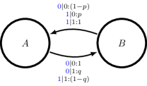
Figure 5: The Maxwellian ratchet’s transducer.

We can drive this ratchet (transducer) with any input, but for comparison with previous work, we drive it with the memoryless biased coin process just introduced and shown in Fig. 4. The resulting unifilar HMM for the output string is shown in Fig. 6. The corresponding symbol-labeled transition matrices are:

$$T^{\prime(0)} =\left[\begin{array}[]{cccc}0&(1-p)b\\ b+q(1-b)&0\end{array}\right]~{},~{}\text{and}$$ (41)

$$T^{\prime(1)} =\left[\begin{array}[]{cccc}0&1-(1-p)b\\ (1-q)(1-b)&0\end{array}\right]~{}.$$ (44)

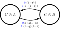
Figure 6: Unifilar HMM for the output string generated by the ratchet driven by a coin with bias $b$.

Using these we can complete our validation of the proposed Second Law, by exactly calculating the entropy rate of the output string. We find:

$$h_{\mu}^{\prime} =\lim_{N\rightarrow\infty}\operatorname{H}[Y^{\prime}_{N}|Y^{\prime}_{0:N}]$$

$$=\lim_{N\rightarrow\infty}\operatorname{H}[Y^{\prime}_{N}|S_{N}]$$

$$=\frac{\operatorname{H}(b(1-p))}{2}+\frac{\operatorname{H}((1-b)(1-q))}{2}~{}.$$ (45)

We note that this is less than or equal to the (unconditioned) single-symbol entropy for the output process:

$$h_{\mu}^{\prime} \leq\operatorname{H}[Y^{\prime}_{0}]$$

$$=\operatorname{H}\left((b(1-p)+(1-b)(1-q))/2\right)~{}.$$ (46)

Any difference between $h_{\mu}^{\prime}$ and single-symbol entropy $\operatorname{H}[Y_{0}]$ indicates correlations that the ratchet created in the output from the uncorrelated input string. In short, the entropy rate gives a more accurate picture of how information is flowing between bit strings and the heat bath. And, as we now demonstrate, the entropy rate leads to correctly identifying important classes of ratchet thermodynamic functioning—functionality the single-symbol entropy misses.

V Thermodynamic Functionality

Let’s step back to review and set context for exploring the ratchet’s thermodynamic functionality as we vary its parameters. Our main results are analytical, provided in closed-form. First, we derived a modified version of the Second Law of Thermodynamics for information ratchets in terms of the difference between the Kolmogorov-Sinai entropy of the input and output strings:

$$\langle W\rangle\leq k_{\text{B}}T\ln 2\,\Delta h_{\mu}~{},$$ (47)

where $\Delta h_{\mu}=h_{\mu}^{\prime}-h_{\mu}$. The improvement here takes into account correlations within the input string and those in the output string actively generated by the ratchet during its operation. From basic information-theoretic identities we know this bound is stricter for memoryless inputs than previous relations [64] that ignored correlations. However, by how much? And, this brings us to our second main result. We gave analytic expressions for both the input and output entropy rates and the work done by the Demon. Now, we are ready to test that the bound is satisfied and to see how much stricter it is than earlier approximations.

We find diverse thermodynamic behaviors as shown in Figure 7, which describes ratchet thermodynamic function at input bias $b=0.9$. We note that there are analogous behaviors for all values of input bias.

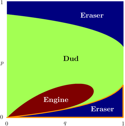
Figure 7: Information ratchet thermodynamic functionality at input bias $b=0.9$: Engine: $(p,q)$ such that $0<\langle W\rangle\leq k_{\text{B}}T\ln 2\,\Delta h_{\mu}$. Eraser: $(p,q)$ such that $\langle W\rangle\leq k_{\text{B}}T\ln 2\,\Delta h_{\mu}<0$. Dud: $(p,q)$ such that $\langle W\rangle\leq 0\leq k_{\text{B}}T\ln 2\,\Delta h_{\mu}$.

We identified three possible behaviors for the ratchet: Engine, Dud, and Eraser. Nowhere does the ratchet violate the rule $\langle W\rangle\leq k_{\text{B}}T\ln 2\,\Delta h_{\mu}$. The engine regime is defined by $(p,q)$ for which $k_{\text{B}}T\ln 2\,\Delta h_{\mu}\geq\langle W\rangle>0$ since work is positive. This is the only condition for which the ratchet extracts work. The eraser regime is defined by $0>k_{\text{B}}T\ln 2\,\Delta h_{\mu}\geq\langle W\rangle$, meaning that work is extracted from the work reservoir while the uncertainty in the bit string decreases. In the dud regime, those $(p,q)$ for which $k_{\text{B}}T\ln 2\,\Delta h_{\mu}\geq 0\geq\langle W\rangle$, the ratchet is neither able to erase information nor is it able to do useful work.

At first blush, these are the same behavior types reported by Ref. [43], except that we have stronger bounds on the work now with $k_{\text{B}}T\ln 2\,\Delta h_{\mu}$, compared to the single-symbol entropy approximation. The stricter bound gives deeper insight into ratchet functionality. To give a concrete comparison, Fig. 8 plots the single-symbol entropy difference $\Delta\operatorname{H}[Y_{0}]$ and the entropy rate difference $\Delta h_{\mu}$, with a flat surface identifying zero entropy change, for all $p$ and $q$ and at $b=0.9$.

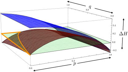
Figure 8: Exact entropy rate difference $\Delta h_{\mu}$ (red) is a much stricter bound on work than the difference in single-symbol entropy $\Delta\operatorname{H}[Y_{0}]$ (blue). The zero surface (light green) highlights where both entropies are greater than zero and so is an aid to identifying functionalities.

In the present setting where input symbols are uncorrelated, the blue $\Delta\!\operatorname{H}[Y_{0}]$ surface lies above the red $\Delta h_{\mu}$ surface for all parameters, confirming that the single-symbol entropy difference is always greater than the entropy rate difference. It should also be noted for this choice of input bias $b$ and for larger $p$, $\Delta\!\operatorname{H}[Y_{0}]$ and $\Delta h_{\mu}$ are close, but they diverge for smaller $p$. They diverge so much, however, that looking only at single-symbol entropy approximation misses an entire low-$p$ region, highlighted in orange in Fig. 8 and 7, where $\Delta h_{\mu}$ dips below zero and the ratchet functions as eraser.

The orange-outlined low-$p$ erasure region is particularly interesting, as it hosts a new functionality not previously identified: The ratchet removes multiple-bit uncertainty, effectively erasing incoming bits by adding temporal order, all the while increasing the uncertainty in individual incoming bits. The existence of this mode of erasure is highly counterintuitive in light of the fact the Demon interacts with only one bit at a time. In contrast, operation in the erasure region at high $p$, like that in previous Demons, simply reduces single-bit uncertainty. Moreover, the low-$p$ erasure region lies very close to the region where ratchet functions as an engine, as shown in Fig. 7. As one approaches $(p,q)=(0,0)$ the eraser and engine regions become arbitrarily close in parameter space. This is a functionally meaningful region, since the device can be easily and efficiently switched between distinct modalities—an eraser or an engine.

In contrast, without knowing the exact entropy rate, it appears that the engine region of the ratchet’s parameter space is isolated from the eraser region by a large dud region and that the ratchet is not tunable. Thus, knowing the correlations between bits in the output string allows one to predict additional functionality that otherwise is obscured when one only considers the single-symbol entropy of the output string.

As alluded to above, we can also consider structured input strings generated by memoryful processes, unlike the memoryless biased coin. While correlations in the output string are relevant to the energetic behavior of this ratchet, it turns out that input string correlations are not. The work done by the ratchet depends only on the input’s single-symbol bias $b$. That said, elsewhere we will explore more intelligent ratchets that take advantage of input string correlations to do additional work.

Conclusion

Thermodynamic systems that include information reservoirs as well as thermal and work reservoirs are an area of growing interest, driven in many cases by biomolecular chemistry or nanoscale physics and engineering. With the ability to manipulate thermal systems on energy scales closer and closer to the level of thermal fluctuations $k_{\text{B}}T$, information becomes critical to the flow of energy. Our model of a ratchet and a bit string as the information reservoir is very flexible and our methods showed how to analyze a broad class of such controlled thermodynamic systems. Central to identifying thermodynamic functionality was our deriving Eq. (5), based on the control system’s Kolmogorov-Sinai entropy, that holds in all situations of memoryful or memoryless ratchets and correlated or uncorrelated input processes and that typically provides the tightest quantitative bound on work. This improvement comes directly from tracking Demon information production over system trajectories, not from time-local, configurational entropies.

Though its perspective and methods were not explicitly highlighted, computational mechanics [65] played a critical role in the foregoing analyses, from its focus on structure and calculating all system component correlations to the technical emphasis on unifilarity in Demon models. Its full impact was not fully explicated here and is left to sequels and sister works. Two complementary computational mechanics analyses of information engines come to mind, in this light. The first is Ref. [16]’s demonstration that the chaotic instability in Szilard’s Engine, reconceived as a deterministic dynamical system, is key to its ability to extract heat from a reservoir. This, too, highlights the role of Kolmogorov-Sinai dynamical entropy. Another is the thorough-going extension of fluctuation relations to show how intelligent agents can harvest energy when synchronizing to the fluctuations from a structured environment [61].

This is to say, in effect, the foregoing showed that computational mechanics is a natural framework for analyzing a ratchet interacting with an information reservoir to extract work from a thermal bath. The input and output strings that compose the information reservoir are best described by unifilar HMM generators, since they allow for exact calculation of any informational property of the strings, most importantly the entropy rate. In fact, the control system components are the $\epsilon$-machines and $\epsilon$-transducers of computational mechanics [65, 62].

By allowing one to exactly calculate the asymptotic entropy rate, we identified more functionality in the effective thermodynamic $\epsilon$-transducers than previous methods can reveal. Two immediate consequences were that we identified a new kind of thermodynamic eraser and found that our ratchet is easily tunable between an eraser and an engine—functionalities suggesting that real-world ratchets exhibit memory to take advantage of correlated environmental fluctuations, as well as hinting at useful future engineering applications.

Appendix A Derivation of Eq. (5)

Here, we reframe the Second Law of Thermodynamics, deriving an expression of it that makes only one assumption about the information ratchet operating along the bit string: the ratchet accesses only a finite number of internal states. This constraint is rather mild and, thus, the bounds on thermodynamic functioning derived from the new Second Law apply quite broadly.

The original Second Law of Thermodynamics states that the total change in entropy of an isolated system must be nonnegative over any time interval. By considering a system composed of a thermal reservoir, information reservoir, and ratchet, in the following we derive an analog in terms of rates, rather than total configurational entropy changes.

Due to the Second Law, we insist that the change in thermodynamic entropy of the closed system is positive for any number $N$ of time steps. If $X$ denotes the ratchet, $Y$ the bit string, and $Z$ the heat bath, this assumption translates to:

$$\triangle S[X,Y,Z]\geq 0~{}.$$ (48)

Note that we do not include a term for the weight (a mechanical energy reservoir), since it does not contribute to the thermodynamic entropy. Expressing the thermodynamic entropy $S$ in terms the Shannon entropy of the random variables $S[X,Y,Z]=k_{\text{B}}\ln 2\operatorname{H}[X,Y,Z]$, we have the condition:

$$\triangle\!\operatorname{H}[X,Y,Z]\geq 0~{}.$$ (49)

To be more precise, this is true over any number of time steps $N$. If we have our system $X$, we denote the random variable for its state at time step $N$ by $X_{N}$. The information reservoir $Y$ is a semi-infinite string. At time zero, the string is composed entirely of the bits of the input process, for which the random variable is denoted $Y_{0:\infty}$. The ratchet transduces these inputs, starting with $Y_{0}$ and generating the output bit string, the entirety of which is expressed by the random variable $Y^{\prime}_{0:\infty}$. At the $N$th time step, the first $N$ bits of the input $Y$ have been converted into the first $N$ bits of the output $Y^{\prime}$, so the random variable for the input-output bit string is $Y_{N:\infty}\otimes Y^{\prime}_{0:N}$. Thus, the change in entropy from the initial time to the $N$th time step is:

$$\triangle\operatorname{H}_{N}[X,Y,Z] =\operatorname{H}[X_{N},Y_{N:\infty},Y^{\prime}_{0:N},Z_{N}]$$

$$\quad\quad-\operatorname{H}[X_{0},Y_{0:\infty},Z_{0}]$$ (50)

$$=\operatorname{H}[X_{N},Y_{N:\infty},Y^{\prime}_{0:N}]+\operatorname{H}[Z_{N}]$$

$$\quad\quad-\operatorname{I}[X_{N},Y_{N:\infty},Y^{\prime}_{0:N};Z_{N}]$$

$$\quad\quad-\operatorname{H}[X_{0},Y_{0:\infty}]-\operatorname{H}[Z_{0}]$$

$$\quad\quad+\operatorname{I}[X_{0},Y_{0:\infty};Z_{0}]~{}.$$ (51)

Note that the internal states of an infinite heat bath do not correlate with the environment, since they have no memory of the environment. This means the mutual informations $\operatorname{I}[X_{N},Y_{N:\infty},Y^{\prime}_{0:N};Z_{N}]$ and $\operatorname{I}[X_{0},Y_{0:\infty};Z_{0}]$ of the thermal reservoir $Z$ with the bit string $Y$ and ratchet $X$ vanish. Also, note that the change in thermal bath entropy can be expressed in terms of the heat dissipated $Q_{N}$ over the $N$ time steps:

$$\triangle\!\operatorname{H}[Z] =\operatorname{H}[Z_{N}]-\operatorname{H}[Z_{0}]$$

$$=Q_{N}/k_{\text{B}}T\ln 2~{}.$$ (52)

Thus, the Second Law naturally separates into energetic terms describing the change in the heat bath and information terms describing the ratchet and bit strings:

$$\triangle\operatorname{H}_{N}[X,Y,Z] =\frac{Q_{N}}{k_{B}T\,\ln 2}$$ (53)

$$\quad\quad+\operatorname{H}[X_{N},Y_{N:\infty},Y^{\prime}_{0:N}]-\operatorname{H}[X_{0},Y_{0:\infty}]~{}.$$

Since $\triangle\operatorname{H}\geq 0$, we can rewrite this as an entirely general lower bound on the dissipated heat over a length $N\tau$ time interval, recalling that $\tau$ is the ratchet-bit interaction time:

$$Q_{N}\geq k_{B}T\,\ln 2\left(\operatorname{H}[X_{0},Y_{0:\infty}]-\operatorname{H}[X_{N},Y_{N:\infty},Y^{\prime}_{0:N}]\right)~{}.$$ (54)

This bound is superficially similar to Eq. (6), but it’s true in all cases, as we have not yet made any assumptions about the ratchet. However, its informational quantities are difficult to calculate for large $N$ and, in their current form, do not give much insight. Thus, we look at the infinite-time limit in order tease out hidden properties.

Over a time interval $N\tau$, the average heat dissipated per ratchet cycle is $Q_{N}/N$. When we classify an engine’s operation, we usually quantify energy flows that neglect transient dynamics. These are just the heat dissipated per cycle over infinite time $\langle Q\rangle=\lim_{N\rightarrow\infty}Q_{N}/N$, which has the lower bound:

$$\langle Q\rangle\geq\lim_{N\rightarrow\infty}k_{B}T\,\ln 2\frac{H[X_{0},Y_{0:\infty}]-H[X_{N},Y_{N:\infty},Y^{\prime}_{0:N}]}{N}.$$ (55)

Assuming the ratchet has a finite number of internal states, each with finite energy, then the bound can be simplified and written in terms of work. In this case, the average work done is the opposite of the average dissipated heat: $\langle W\rangle=-\langle Q\rangle$. And so, it has the upper bound:

$$\langle W\rangle\leq k_{B}T\,\ln 2 \lim_{N\rightarrow\infty}\bigg{(}\frac{H[Y_{N:\infty},Y^{\prime}_{0:N}]-H[Y_{0:\infty}]}{N}$$

$$+\frac{H[X_{N}]-H[X_{0}]}{N}$$ (56)

$$+\frac{I[X_{0};Y_{0:\infty}]-I[X_{N};Y_{N:\infty},Y^{\prime}_{0:N}]}{N}\bigg{)},$$

where the joint entropies are expanded in terms of their single-variable entropies and mutual informations.

The entropies over the initial $X_{0}$ and final $X_{N}$ ratchet state distributions monitor the change in ratchet memory—time-dependent versions of its statistical complexity $C_{\mu}(N)=\operatorname{H}[X_{N}]$ [65]. This time dependence can be used to monitor how and when the ratchet synchronizes to the incoming sequence, recognizing a sequence’s temporal correlations. However, since we assumed that the ratchet has finite states, the ratchet state-entropy and also mutual information terms involving it are bounded above by the logarithm of the number states. And so, they go to zero as $N\to\infty$, leaving the expression:

$$\langle W\rangle \leq k_{B}T\,\ln 2\lim_{N\rightarrow\infty}\bigg{(}\frac{H[Y_{N:\infty},Y^{\prime}_{0:N}]-H[Y_{0:\infty}]}{N}\bigg{)}~{}.$$ (57)

With this, we have a very general upper bound for the work done by the ratchet in terms of just the input and output string variables.

Once again, we split the joint entropy term into it’s components:

$$\langle W\rangle\leq k_{B}T\,\ln 2\lim_{N\rightarrow\infty} \bigg{(}\frac{H[Y_{N:\infty}]-H[Y_{0:\infty}]}{N}$$ (58)

$$\quad+\frac{H[Y^{\prime}_{0:N}]}{N}-\frac{I[Y_{N:\infty};Y^{\prime}_{0:N}]}{N}\bigg{)}~{}.$$

In this we identify the output process’s entropy rate $h_{\mu}^{\prime}=\lim_{N\rightarrow\infty}\operatorname{H}[Y^{\prime}_{0:N}]/N$. While $\lim_{N\rightarrow\infty}\big{(}\operatorname{H}[Y_{N:\infty}]-\operatorname{H}[Y_{0:\infty}]\big{)}/N$ looks unfamiliar, it is actually the negative entropy rate $h_{\mu}$ of the input process, so we find that:

$$\langle W\rangle \leq k_{B}T\,\ln 2\bigg{(}h^{\prime}_{\mu}-h_{\mu}-\lim_{N\rightarrow\infty}\frac{I[Y_{N:\infty};Y^{\prime}_{0:N}]}{N}\bigg{)}.$$ (59)

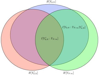
Figure 9: The $N$ most recent variables of the input process shield the $N$ variables of output from the rest of the input variables.

To understand the mutual information term, note that $Y^{\prime}_{0:N}$ is generated from $Y_{0:N}$, so it is independent of $Y_{N:\infty}$ conditioned on $Y_{0:N}$. Essentially, $Y_{0:N}$ causally shields $Y^{\prime}_{0:N}$ from $Y_{N:\infty}$, as shown in information diagram [66] of Fig 9. This means:

$$\operatorname{I}[Y_{N:\infty};Y^{\prime}_{0:N}]=\operatorname{I}[Y_{N:\infty};Y_{0:N}]-\operatorname{I}[Y_{N:\infty};Y_{0:N}|Y^{\prime}_{0:N}]~{}.$$ (60)

This, in turn, gives: $\operatorname{I}[Y_{N:\infty};Y_{0:N}]\geq\operatorname{I}[Y_{N:\infty};Y^{\prime}_{0:N}]\geq 0$. Thus, we find the input process’s excess entropy ${\bf E}$ [55]:

$$\lim_{N\rightarrow\infty}\operatorname{I}[Y_{N:\infty};Y^{\prime}_{0:N}] \leq\lim_{N\rightarrow\infty}\operatorname{I}[Y_{N:\infty};Y_{0:N}]$$

$$={\bf E}~{}.$$ (61)

However, dividing by $N$ it’s contribution vanishes:

$$\lim_{N\rightarrow\infty}\frac{I[Y_{N:\infty};Y_{0:N}]}{N} =\lim_{N\rightarrow\infty}\left(\frac{H[Y_{0:N}]}{N}-\frac{H[Y_{0:N}|Y_{N:\infty}]}{N}\right)$$

$$=h_{\mu}-h_{\mu}$$

$$=0~{}.$$ (62)

Thus, we are left with the inequality of Eq. (5):

$$\langle W\rangle\leq k_{B}T\,\ln 2\left(h_{\mu}^{\prime}-h_{\mu}\right)~{};$$ (63)

derived with minimal assumptions. Also, the appearance of the statistical complexity and excess entropy, whose contributions this particular derivation shows are asymptotically small, does indicate the potential role of correlations in the input for finite time—times during which the ratchet synchronizes to the incoming information [67].

One key difference between Eq. (63) (equivalently, Eq. (5)) and the more commonly used bound in Eq. (6), with the change in single-variable configurational entropy $\operatorname{H}[Y^{\prime}_{0}]-\operatorname{H}[Y_{0}]$, is that the former bound is true for all finite ratchets and takes into account the production of information over time via the Kolmogorov-Sinai entropies $h_{\mu}$ and $h_{\mu}^{\prime}$. More generally, we do not look at single-step changes in configurational entropies—$\operatorname{H}[X_{N-1},Y_{N-1},Z_{N-1}]\to\operatorname{H}[X_{N},Y_{N},Z_{N}]$—but rather the rate of production of information $\operatorname{H}[W_{N}|\ldots W_{N-2},W_{N-1}]$, where $W_{N}=(X_{N},Y_{N},Z_{N})$. This global dynamical entropy rate has contributions from output rate $h_{\mu}^{\prime}$ and input rate $h_{\mu}$. This again indicates how Eq. (6) approximates Eq. (63).

There are several special cases where the single-variable bound of Eq. (6) applies. In the case where the input is uncorrelated, it holds, but it is a weaker bound than Eq. (5) using entropy rates. Also, in the case when the ratchet has no internal states and so is memoryless, Eq. (6) is satisfied. Interestingly, either it or Eq. (63) can be quantitatively stricter in this special case. However, in the most general case where the inputs are correlated and the ratchet has memory, the bound using single-variable entropy is incorrect, since there are cases where it is violated [68]. Finally, when the input-bit-ratchet interaction time $\tau$ grows the ratchet spends much time thermalizing. The result is that the output string becomes uncorrelated with the input and so the ratchet is effectively memoryless. Whether by assumption or if it arises as the effective behavior, whenever the ratchet is memoryless, it is ignorant of temporal correlations and so it and the single-symbol entropy bounds are of limited physical import. These issues will be discussed in detail in future works, but as a preview see Ref. [68].

Appendix B Designing Ratchet Energetics

Figure 3 is one of the simplest information transducers for which the outcomes are unifilar for uncorrelated inputs, resulting in the fact that the correlations in the outgoing bits can be explicitly calculated. As this calculation was a primary motivation in our work, we introduced the model in Fig. 3 first and, only then, introduced the associated energetic and thermodynamic quantities, as in Fig. 2. The introduction of energetic and thermodynamic quantities for an abstract transducer (as in Fig. 3), however, is not trivial. Given a transducer topology (such as the reverse “Z” shape of the current model), there are multiple possible energy schemes of which only a fraction are consistent with all possible values of the associated transition probabilities. However, more than one scheme is generally possible.

To show that only a fraction of all possible energetic schemes are consistent with all possible parameter values, consider the case where the interaction energy between the ratchet and a bit is zero, as in Ref. [43]. In our model, this implies $\beta=0$, or equivalently, $p=q=0$ (from Eq. (16)). In other words, we cannot describe our model, valid for all values $0<p,q<1$, by the energy scheme in Fig. 2 with $\beta=0$. This is despite the fact that we have two other independent parameters $\alpha$ and $w$.

To show that, nonetheless, more than one scheme is possible, imagine the case with $\alpha=\beta=0$. Instead of just one mass, consider three masses such that, whenever the transitions $A\otimes 0\rightarrow B\otimes 0$, $B\otimes 0\rightarrow A\otimes 1$, and $A\otimes 1\rightarrow B\otimes 1$ take place, we get works $k_{\text{B}}T\widetilde{W}_{1}$, $k_{\text{B}}T\widetilde{W}_{2}$, and $k_{\text{B}}T\widetilde{W}_{3}$, respectively. We lose the corresponding amounts of work for the reverse transitions. This picture is consistent with the abstract model of Fig. 3 if the following requirements of detailed balance are satisfied:

$$\frac{1}{1-p} =\frac{M_{A\otimes 0\rightarrow B\otimes 0}}{M_{B\otimes 0\rightarrow A\otimes 0}}=e^{-\widetilde{W}_{1}}~{},$$ (64)

$$\frac{p}{q} =\frac{M_{B\otimes 0\rightarrow A\otimes 1}}{M_{A\otimes 1\rightarrow B\otimes 0}}=e^{-\widetilde{W}_{2}}~{},~{}\text{and}$$ (65)

$$1-q =\frac{M_{A\otimes 1\rightarrow B\otimes 1}}{M_{B\otimes 1\rightarrow A\otimes 1}}=e^{-\widetilde{W}_{3}}~{}.$$ (66)

Existence of such an alternative scheme illustrates the fact that given the abstract model of Fig. 3, there is more than one possible consistent energy scheme. We suggest that this will allow for future engineering flexibility.

References

- [1] D. J. Evans, E. G. D. Cohen, and G. P. Morriss. Probability of second law violations in shearing steady flows. Phys. Rev. Lett., 71:2401–2404, 1993.
- [2] D. J. Evans and D. J. Searles. Equilibrium microstates which generate second law violating steady states. Phys. Rev. E, 50:1645, 1994.
- [3] G. Gallavotti and E. G. D. Cohen. Dynamical ensembles in nonequilibrium statistical mechanics. Phys. Rev. Lett., 74:2694–2697, 1995.
- [4] J. Kurchan. Fluctuation theorem for stochastic dynamics. J. Phys. A: Math. Gen., 31:3719, 1998.
- [5] G. E. Crooks. Nonequilibrium measurements of free energy differences for microscopically reversible markovian systems. J. Stat. Phys., 90(5/6):1481–1487, 1998.
- [6] J. L. Lebowitz and H. Spohn. A Gallavotti-Cohen-type symmetry in the large deviation functional for stochastic dynamics. J. Stat. Phys., 95:333, 1999.
- [7] D. Collin, F. Ritort, C. Jarzynski, S. B. Smith, I. Tinoco Jr., and C. Bustamante. Verification of the Crooks fluctuation theorem and recovery of RNA folding free energies. Nature, 437:231, 2005.
- [8] H. Leff and A. Rex. Maxwell’s Demon 2: Entropy, Classical and Quantum Information, Computing. Taylor and Francis, New York, 2002.
- [9] K. Maruyama, F. Nori, and V. Vedral. Colloquium: The physics of Maxwell’s demon and information. 2009, 81:1, Rev. Mod. Phys.
- [10] M. v. Smoluchowski. Drei vorträge über diffusion, etc. Physik. Zeit., XVII:557–571, 1916.
- [11] L. Szilard. On the decrease of entropy in a thermodynamic system by the intervention of intelligent beings. Z. Phys., 53:840–856, 1929.
- [12] R. Landauer. Irreversibility and heat generation in the computing process. IBM J. Res. Develop., 5(3):183–191, 1961.
- [13] O. Penrose. Foundations of statistical mechanics; a deductive treatment. Pergamon Press, Oxford, 1970.
- [14] C. H. Bennett. Thermodynamics of computation - a review. Intl. J. Theo. Phys., 21:905, 1982.
- [15] A. B rut, A. Arakelyan, A. Petrosyan, S. Ciliberto, R. Dillenschneider, and E. Lutz. Experimental verification of landauer s principle linking information and thermodynamics. Nature, 483:187, 2012.
- [16] A. B. Boyd and J. P. Crutchfield. Demon dynamics: Deterministic chaos, the Szilard map, and the intelligence of thermodynamic systems. 2015. SFI Working Paper 15-06-019; arxiv.org:1506.04327 [cond-mat.stat- mech].
- [17] S. Deffner and C. Jarzynski. Information processing and the second law of thermodynamics: An inclusive, Hamiltonian approach. Phys. Rev. X, 3:041003, 2013.
- [18] A. C. Barato and U. Seifert. Stochastic thermodynamics with information reservoirs. Phys. Rev. E, 90:042150, 2014.
- [19] T. M. Cover and J. A. Thomas. Elements of Information Theory. Wiley-Interscience, New York, second edition, 2006.
- [20] H. Touchette and S. Lloyd. Information-theoretic limits of control. Phys. Rev. Lett., 84:1156, 2000.
- [21] F. J. Cao, L. Dinis, and J. M. R. Parrondo. Feedback control in a collective flashing ratchet. Phys. Rev Lett., 93:040603, 2004.
- [22] T. Sagawa and M. Ueda. Generalized Jarzynski equality under nonequilibrium feedback control. Phys. Rev. Lett., 104:090602, 2010.
- [23] S. Toyabe, T. Sagawa, M. Ueda, E. Muneyuki, and M. Sano. Experimental demonstration of information-to-energy conversion and validation of the generalized Jarzynski equality. Nature Physics, 6:988–992, 2010.
- [24] M. Ponmurugan. Generalized detailed fluctuation theorem under nonequilibrium feedback control. Phys. Rev. E, 82:031129, 2010.
- [25] J. M. Horowitz and S. Vaikuntanathan. Nonequilibrium detailed fluctuation theorem for repeated discrete feedback. Phys. Rev. E, 82:061120, 2010.
- [26] J. M. Horowitz and J. M. R. Parrondo. Thermodynamic reversibility in feedback processes. Europhys. Lett., 95:10005, 2011.
- [27] L. Granger and H. Krantz. Thermodynamic cost of measurements. Phys. Rev. E, 84:061110, 2011.
- [28] D. Abreu and U. Seifert. Extracting work from a single heat bath through feedback. Europhys. Lett., 94:10001, 2011.
- [29] S. Vaikuntanathan and C. Jarzynski. Modeling Maxwell’s demon with a microcanonical szilard engine. Phys. Rev. E, 83:061120, 2011.
- [30] A. Abreu and U. Seifert. Thermodynamics of genuine nonequilibrium states under feedback control. Phys. Rev. Lett., 108:030601, 2012.
- [31] A. Kundu. Nonequilibrium fluctuation theorem for systems under discrete and continuous feedback control. Phys. Rev. E, 86:021107, 2012.
- [32] T. Sagawa and M. Ueda. Fluctuation theorem with information exchange: Role of correlations in stochastic thermodynamics. Phys. Rev. Lett., 109:180602, 2012.
- [33] L. B. Kish and C. G. Granqvist. Energy requirement of control: Comments on Szilard’s engine and Maxwell’s demon. Europhys. Lett., 98:68001, 2012.
- [34] S. Ito and T. Sagawa. Information thermodynamics on causal networks. Phys. Rev. Lett., 111:180603, 2013.
- [35] D. Hartich, A. C. A. C. Barato, and U. Seifert. Stochastic thermodynamics of bipartite systems: Transfer entropy inequalities and a Maxwell’s demon interpretation. J. Stat. Mech.: Theor. Exp., 2013:P02016, 2014.
- [36] J. M. Horowitz and M. Esposito. Thermodynamics with continuous information flow. Phys. Rev. X, 4:031015, 2014.
- [37] J. M. Horowitz. Multipartite information flow for multiple Maxwell demons. J. Stat. Mech.: Theor. Exp., 2015:P03006, 2015.
- [38] M. Esposito and G. Schaller. Stochastic thermodynamics for “Maxwell demon” feedbacks. Europhys. Lett., 99:30003, 2012.
- [39] P. Strasberg, G. Schaller, T. Brandes, and M. Esposito. Thermodynamics of a physical model implementing a Maxwell demon. Phys. Rev. Lett., 110:040601, 2013.
- [40] J. M. Horowitz, T. Sagawa, and J. M. R. Parrondo. Imitating chemical motors with mptimal information motors. Phys. Rev. Lett., 111:010602, 2013.
- [41] A. C. Barato and U. Seifert. Unifying three perspectives on information processing in stochastic thermodynamics. Phys. Rev. Lett., 112:090601, 2014.
- [42] J. M. Horowitz and H. Sandberg. Second-law-like inequalities with information and their interpretations. New J. Phys., 16:125007, 2014.
- [43] D. Mandal and C. Jarzynski. Work and information processing in a solvable model of Maxwell’s demon. Proc. Natl. Acad. Sci. USA, 109(29):11641–11645, 2012.
- [44] D. Mandal, H. T. Quan, and C. Jarzynski. Maxwell’s refrigerator: An exactly solvable model. Phys. Rev. Lett., 111:030602, 2013.
- [45] A. C. Barato and U. Seifert. An autonomous and reversible Maxwell’s demon. Europhys. Lett., 101:60001, 2013.
- [46] J. Hoppenau and A. Engel. On the energetics of information exchange. Europhys. Lett., 105:50002, 2014.
- [47] Z. Lu, D. Mandal, and C. Jarzynski. Engineering Maxwell’s demon. Physics Today, 67(8):60–61, January 2014.
- [48] J. Um, H. Hinrichsen, C. Kwon, and H. Park. Total cost of operating an information engine. arXiv:1501.03733 [cond-mat.stat-mech], 2015.
- [49] J. R. Dorfman. An Introduction to Chaos in Nonequilibrium Statistical Mechanics. Cambridge University Press, Cambridge, United Kingdom, 1999.
- [50] B. Alberts, A. Johnson, J. Lewis, D. Morgan, and M. Raff. Molecular Biology of the Cell. Garland Science, New York, sixth edition, 2014.
- [51] L. Brillouin. Life, thermodynamics, and cybernetics. Am. Scientist, 37:554–568, 1949.
- [52] H. R. Lewis and C. H. Papadimitriou. Elements of the Theory of Computation. Prentice-Hall, Englewood Cliffs, N.J., second edition, 1998.
- [53] P. Strasberg, J. Cerrillo, G. Schaller, and T. Brandes. Thermodynamics of stochastic Turing machines. arXiv:1506.00894, 2015.
- [54] C. Moore. Unpredictability and undecidability in dynamical systems. Phys. Rev. Lett., 64:2354, 1990.
- [55] J. P. Crutchfield and D. P. Feldman. Regularities unseen, randomness observed: Levels of entropy convergence. CHAOS, 13(1):25–54, 2003.
- [56] D. Blackwell. The entropy of functions of finite-state Markov chains. In Transactions of the first Prague conference on information theory, Statistical decision functions, Random processes, volume 28, pages 13–20. Publishing House of the Czechoslovak Academy of Sciences, Prague, Czechoslovakia, 1957. Held at Liblice near Prague from November 28 to 30, 1956.
- [57] B. Marcus, K. Petersen, and T. Weissman, editors. Entropy of Hidden Markov Process and Connections to Dynamical Systems, volume 385 of Lecture Notes Series. London Mathematical Society, 2011.
- [58] Reference [43]’s appendix suggests Eq. (5) without any detailed proof. An integrated version appeared also in Ref. [59] for the special case of memoryless demons. Our App. A gives a more general proof of Eq. (5) that, in addition, accounts for memory.
- [59] N. Merhav. Sequence complexity and work extraction. J. Stat. Mech., page P06037, 2015.
- [60] A. Chapman and A. Miyake. How can an autonomous quantum Maxwell demon harness correlated information? arXiv:1506.09207, 2015.
- [61] P. M. Riechers and J. P. Crutchfield. Thermodynamics of adaptation: Broken reversibility, fluctuations, and path entropies when controlling structured out-of-equilibrium systems. in preparation, 2015.
- [62] N. Barnett and J. P. Crutchfield. Computational mechanics of input-output processes: Structured transformations and the -transducer. J. Stat. Phys., 161(2):404–451, 2015.
- [63] C. E. Shannon. A mathematical theory of communication. Bell Sys. Tech. J., 27:379–423, 623–656, 1948.
- [64] C. Jarzynski. Nonequilibrium equality for free energy differences. Phys. Rev. Lett., 78(14):2690–2693, 1997.
- [65] J. P. Crutchfield. Between order and chaos. Nature Physics, 8(January):17–24, 2012.
- [66] R. W. Yeung. Information Theory and Network Coding. Springer, New York, 2008.
- [67] J. P. Crutchfield, C. J. Ellison, J. R. Mahoney, and R. G. James. Synchronization and control in intrinsic and designed computation: An information-theoretic analysis of competing models of stochastic computation. CHAOS, 20(3):037105, 2010.
- [68] D. Mandal, A. B. Boyd, and J. P. Crutchfield. Memoryless thermodynamics? A reply. 2015. SFI Working Paper 15-08-031; arxiv.org:1508.03311 [cond-mat.stat-mech].