Correspondence Factor Analysis of Big Data Sets: A Case Study of 30 Million Words; and Contrasting Analytics using Apache Solr and Correspondence Analysis in R

Abstract

We consider a large number of text data sets. These are cooking recipes. Term distribution and other distributional properties of the data are investigated. Our aim is to look at various analytical approaches which allow for mining of information on both high and low detail scales. Metric space embedding is fundamental to our interest in the semantic properties of this data. We consider the projection of all data into analyses of aggregated versions of the data. We contrast that with projection of aggregated versions of the data into analyses of all the data. Analogously for the term set, we look at analysis of selected terms. We also look at inherent term associations such as between singular and plural. In addition to our use of Correspondence Analysis in R, for latent semantic space mapping, we also use Apache Solr. Setting up the Solr server and carrying out querying is described. A further novelty is that querying is supported in Solr based on the principal factor plane mapping of all the data. This uses a bounding box query, based on factor projections.

Technical Report: Table of Contents

• Part 1: Correspondence Factor Analysis of Big Data Sets: A Case Study of 30 Million Words

• 1. Data

• 1.1 General Considerations in Regard to High Dimensional and Massive Datasets

• 1.2 Characteristics of the Data Studied

• 1.3 Distribution of Terms

• 2. Objective of Computational Efficiency: Using Aggregated Subsets to Construct the Factor Space

• 2.1 Introduction

• 2.2 Projection into the Factor Space

• 2.3 The Practical Benefit of a Selected Word Set

• 2.4 Conclusion

• Part 2: Data Analysis of Recipes: Contrasting Analytics using Apache Solr and Correspondence Analysis in R

• 3. About the Data; followed by Correspondence Analysis of All Recipes using a 247 Word Set

• 4. Search Using Solr

• 4.1 Setting Up Data File and Its Description

• 4.2 Running the Server and Updating the Index

• 4.3 Querying and Other Operations

• 4.3.1 Web Browser User Interface

• 4.3.2 Command Line Querying

• 5. Consistency of Solr Searches

• References

• Appendix 1: Sample Recipe

• Appendix 2: 247 Ingredients Used as Attributes in the Correspondence Analysis

• Appendix 3: Alternative Presentation of Plot

• Appendix 4: Correspondence Analysis for Singular/Plural Association and Potentially for Disambiguation

Part 1: Correspondence Factor Analysis of Big Data Sets: A Case Study of 30 Million Words

1 Data

1.1 General Considerations in Regard to High Dimensional and Massive Datasets

Very high dimensional (or equivalently, very low sample size or low $n$) data sets, by virtue of high relative dimensionality alone, have points mostly lying at the vertices of a regular simplex or polygon [4, 11].

In [8], the following issues are posed. Firstly, what should we do, for our analytics, when we have thousands of documents? Correspondence Analysis outputs (and this is the same for other kindred methods, like LSA, latent semantic analysis; PLSA, probabilistic adaptation of LSA using a mixture of multinomial distributions; Factorial Correspondence Analysis (CA); Kohonen maps; or clustering methods) are very huge (much more than the original dataset). What we must therefore do is to display the output in an “intelligent” and friendly way.

1.2 Characteristics of the Data Studied

We explore the following.

• We have 306 collections, labelled by “Recipe via Meal-Master (tm) v8.05”, each with, in principle, 500 recipes.

• (An additional set of 20 collections, relating to “v8.06”, were considered as different, and set aside from this work.)

• There is one exception here: one of the collection files had two recipes less than the usual 500 complement.

• Hence we are dealing with 306 $\times$ 500 recipes (less 2), i.e. 152,998.

• Appendix 1 shows a sample recipe.

• This data, in text, contained: 5,948,739 lines of text; 30,199,625 (whitespace-demarcated) words; and 206,993,672 characters.

• On the 306 recipe collections, comprising 152,998 recipes, we used our term extractor. This listed all terms of one character or more, having first removed punctuation and numeric character. We will use the term “words” for what was extracted. All upper case had been first set to lower case. Abbreviations and acronyms showed up as words, some character combinations did so also following punctuation removal, and all forms of stemming were retained.

  Various misspellings are in the given data. In collection mm066001.mmf, there is: “Grate the zuccini into a calendar (sp)…”. What is intended is “zucchini” and “colander”. Interestingly there are 57 times that “zuccini” appears, and once that “zuccinis” appears.

  While spelt correctly, “zucchini” is present 7155 times, and “zucchinis” is present 56 times. There are various other incorrect words present, with one occurrence each: “azucchini”, “brushingzucchini”, “lambzucchini”, “ofzucchini”, “pzucchini”, “zucchinia”, “zucchiniabout”, “zucchinii”, “zzzucchini”.

  Since we take the data as such, notwithstanding such inaccuracies, it is to be noted that the correct spellings are predominant, and that the misspellings only show up if quite atypical features in the data (such as rare occurrence) are looked into. Let us formulate this as a working principle, or perhaps even a working hypothesis that we have verified in all cases that we have looked into. In the case of large, or very large, numbers of occurrences of entities, the syntactically correct form will predominate.

• From the 152,998 recipes we obtained 101,060 unique words.

• In this list, ranked by decreasing frequency of occurrence, the 5000th ranked word had 162 occurrences; the 15,000th ranked word had 18 occurrences; and at the 56,229th ranked word (56% through the total list of 101,060 ranked words), the frequency of occurrence became thereafter (for higher ranked words), 1.

• The top frequencies of occurrence are as follows:

  and 890294
  the 842542
  to 531633
  in 469003
  with 313588
  of 281320
  recipe 280035
  or 247912
  ts 238309
  for 226514
  until 224481
  add 207146
  tb 200221
  from 193659
  minutes 190880
  by 190815
  on 183287
  salt 162811
  yield 162082
  servings 161098
  meal 155040
  master 152980
  via 149162
  title 148802
  tm 148766
  categories 148612
  into 145565
  sugar 138670
  heat 131846
  water 130211
  pepper 127901
  oil 122997
  chopped 119530
  over 115212
  butter 112329
  at 106300
  sauce 102881
  is 101060
  com 99841
  flour 96793
  stir 91580
  mixture 91484
  about 91279
  it 89491
  cook 87097
  pan 86314
  oz 83908
  garlic 82776
  cream 81633
  place 80825
  cheese 78986
  bowl 76209
  mix 76182
  chicken 75807
  onion 71516
  cut 70808
  lb 68376
  posted 67769
  fresh 66125
  baking 64731
  

• The very final ranked words were as follows:

  zwiebelfleisch 1
  zwirek 1
  zws 1
  zygielbaum 1
  zyla 1
  zylman 1
  zza 1
  zzwc 1
  zzzingers 1
  zzzucchini 1
  

  The second last here arose from this entry in a recipe: “Title: Wing Zzzingers”. The last word comes from this entry in a recipe: “Add zzzucchini, peppers and onion.”.

1.3 Distribution of Terms

A power law (see [7]) is a distribution (e.g. of frequency of occurrence) of the form $x^{-\alpha}$ where constant, for the data, $\alpha>0$; and an exponential law is of the form $e^{-x}$. For a power law, $P(x>x_{0})\sim cx^{-\alpha}$, $c,\alpha>0$. A power law has heavier tails than an exponential distribution. In practice $0\leq\alpha\leq 3$. For such values, $x$ has infinite (i.e. arbitrarily large) variance; and if $\alpha\leq 1$ then the mean of $x$ is infinite.

The density function of a power law is $f(x)=\alpha cx^{-\alpha-1}$, and so $\ln f(x)=-\alpha\ln x+C$, where $C$ is a constant offset. Hence a log-log plot shows a power law as linear. Power laws have been of great importance for modelling networks and other complex data sets (see [2, 16]).

Figure 1 shows a plot of rank (most frequent, through to least frequent, the latter being a very large number of words that occur once only) against the value of the frequency of occurrence. To understand the plot, we use log-log scaling.

In a very similar way to the power law properties of large networks (or file sizes, etc.) we find an approximately linear regime, ending (at the lower right) in a large fan-out region. The slope of the linear region characterizes the power law. We find that the probability of having more than $x$ occurrences per word to be approximately $c/x^{-2.3515}$ for large $x$ (since we find the slope of the fitted line in Figure 1 to be $-2.3515$).

Figure 1: Log-log plot of histogram of word ranks versus frequency of occurrence. This uses 101,060 unique words of one character or more. Summarized in this plot there are 30,199,625 words in total, culled from 152,998 recipes. The line of best fit in the linear regime is used to calculate the power law expression for this data.

2 Objective of Computational Efficiency: Using Aggregated Subsets to Construct the Factor Space

2.1 Introduction

Just how well can Correspondence Analysis carry out the Euclidean, factor determining mapping, if recipes are first aggregated together? One reason for this question is computational time. For analysis of an $n\times m$ data set, with $m$ words and $n$ recipes or recipes collections, then the dual spaces means that we analyze either the data set or its transpose. Eigen-reduction is a cubic process. The computational time for analysis of the $n\times m$ data set is $O(m^{3})$, or for its transpose, $O(n^{3})$. For a selected word set, if we can carry out the main analysis on a smaller $n$, so much the better for us.

Aggregation is just concatenating the recipes. In the entire set of recipes, the number of words (to repeat: of one or more characters in length; punctuation deleted; upper case set to lower case; numerical and accented characters ignored) was 101,060. For initial assessment, we took the top-ranking 1000 words. So this illustrative case, using just 500 recipes, has the recipe set crossed by this 1000-word set, with the frequencies of occurrence tabulated.

We aggregated the 500 recipes into 5 recipe-sets. These comprised recipes 1–100, 101–200, 201–300, 301–400, and 401-500. Each of these 5 recipe-sets had the frequencies of occurrences on the 1000-word set.

Here we analyze two cross-tabulation tables, of dimensions respectively $500\times 1000$, and $5\times 1000$. By construction of the latter, the column sums are identical. Then due to the use of profiles, the average profile is the same in each case. If we represent the data matrix in frequency terms (i.e. the frequencies of occurrences each divided by the grand total), the matrix can be denoted $f_{IJ}=\{f_{ij}|i\in I,j\in J\}$ where $I$ is set of recipes, or of recipe-sets, $J$ is the word-set, $i$ is a recipe or a recipe-set, and $j$ is a word) the column marginal distribution is $f_{J}=\{f_{j}|j\in J\}$, or in summation terms, $\sum_{i\in I}f_{ij}$.

In Correspondence Analysis, the centre or origin of the Euclidean factor space is given by $f_{J}$ in the recipe space, and by $f_{I}$ in the word space, such that we have the following view: starting with a probability distribution $f_{IJ}$ we want to explore how it differs from the product of marginal distributions, $f_{I}f_{J}$, and this in the $\chi^{2}$ metric of centre, the product $f_{I}f_{J}$. This is a decomposition of inertia of clouds in recipe and/or in word space. We have: $M^{2}(N_{I}(J))=M^{2}(N_{J}(I)=\|f_{IJ}-f_{I}f_{J}\|^{2}_{f_{I}f_{J}}=\sum_{i\in I,j\in J}(f_{ij}-f_{i}f_{j})^{2}/f_{i}f_{j}=\sum_{i\in I}f_{i}\|f^{i}_{J}-f_{J}\|^{2}_{f_{J}}=\sum_{j\in J}f_{j}\|f^{j}_{I}-f_{I}\|^{2}_{f_{I}}$ where $f^{i}_{J}=\{f_{ij}/f_{i}\}$.

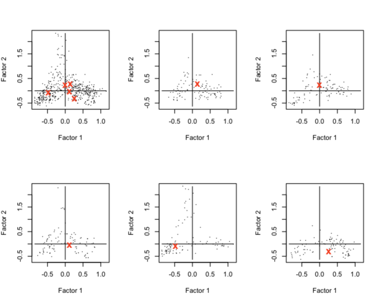
Figure 2: Upper left: projection on principal factor plane of 500 recipes, located at the dots; and the 5 recipe-sets, located at the centres of the x symbols. The analyses were carried out separately. Just to see how the recipe-sets are at the centres of gravity of their associated recipes, displayed here in planar projections, the successive panels show just the recipe-set projected, and the associated 100 recipes, projected as dots.

Figure 2 shows the principal factor display resulting from the Correspondence Analysis of (1) the $500\times 1000$ recipes times words data, and (2) the $5\times 1000$ recipe-sets times words data. Note again that the analyses (the eigen-reductions – determining the factors) were completely independent.

The results of Figure 2 can be explained in the following terms. We have a set of 500 items (the recipes) with quantitative description in a 1000-dimensional space. We have a derived, through concatenating, sets of 5 items in the same 1000-dimensional space. So the resultant Euclidean mappings illustrate well the shared provenance in the two cases. The word analysis is less clear-cut. Given the inherent dimensionality of the Euclidean, factor space is min($n-1,m-1$), we have, on the one hand 1000 words projected into a 499-dimensional space, and on the other hand 1000 words projected into a 4-dimensional space. The locations of a given word in these two spaces are not directly related.

2.2 Projection into the Factor Space

We investigate supplementary elements to expedite the computation. Carry out analysis in a small dimensional space, that nonetheless takes account of all relationships in an aggregated way. Then complete the analysis on all the data by projecting into the Euclidean, factor space.

We took the 306 collected sets of, each, 500 recipes (save for the case of 2 recipes short of this in one such collected set: hence we were dealing with 152,998 recipes). The number of words found in this data (to repeat: of one or more characters in length; punctuation deleted; upper case set to lower case; numerical and accented characters ignored) was 101,060. For initial assessment, we took the top-ranking 1000 words.

The following principles and practices of Correspondence Analysis will now be availed of (see [5, 6, 13]):

• In Correspondence Analysis, all frequency of occurrence values are divided by the grand total (so that allows the viewpoint of empirical probabilities). If the row $i$ mass is then $w_{i}$, the row $i$ profile is the row vector $x_{i}$ with each element divided by $w_{i}$. Now consider the 360-set, which is just all 500 recipes, $x_{i}$, summed. The profile of this set is $\sum x_{i}/\sum w_{i}$ where $i=1,2,\dots,50$. If one recipe is a multiplicative constant of another (i.e. elementwise, for each word), then their profiles are the same.

• The dual space relations allows supplementary rows or columns to be projected, after the fact, into the analysis.

  (In the Latent Semantic Indexing context, “folding in” of newly presented rows or columns, that can be considered as a row or column set that is juxtaposed to the original $I\times J$ matrix, is described in [1]).

• Profiles are analyzed in Correspondence Analysis, meaning that row vector, and column vector, values have been divided by the associated row, or column, total. Consider the row or column total as a mass, as is done in this context. By having all values first divided by the grand total of the rows/columns array, we have all values bounded by 0 and 1. (Note that we require non-negative values for the mass to be workable for us here.) In this way our 306-set of (500) recipes is the weighted mean of the associated recipes

  To see this, consider the given frequency of occurrence data divided by the grand total (over all recipes and words), on the set of recipes, that we will represent by matrix $x$. Consider the 500 recipes that are associated with one of the 306-sets. Without loss of generality, call them $x_{1j},x_{2j},\dots,x_{500,j}$. We will denote one such recipe by $x_{kj}$ and just right now we are most interested in the set $\{x_{kj}|k=1,2,\dots,500;j\in J\}$. $J$ is the set of words. Then the profile of recipe $k$ is $x_{kj}/\sum_{j}x_{kj}$.

  Now consider the 360-set. It is the aggregation (concatenation) of the recipes. So, it is $\sum_{k=1}^{50}x_{kj}$. Its profile is $\sum_{k=1}^{50}x_{kj}/\sum_{k,j}x_{kj}$.

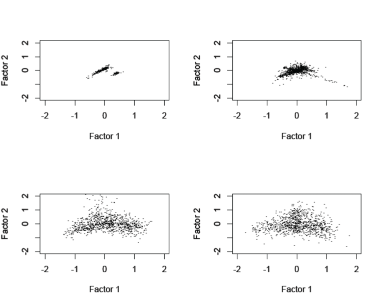
Figure 3: Upper left: 306 collections of 500 (in one case, 498) recipes. Upper right: the top ranked 1000 words used for the 306 collections of recipes. The upper right is the dual space of the upper left. Lower left: the 1000 words for one set of 500 recipes. Lower right: the 1000 words for another set of 500 recipes.

Figure 3 presents an initial look at the use of the top ranked words (in terms of frequency of occurrence in the entire data collection, hence: 306 collections of recipes, or 152,998 recipes).

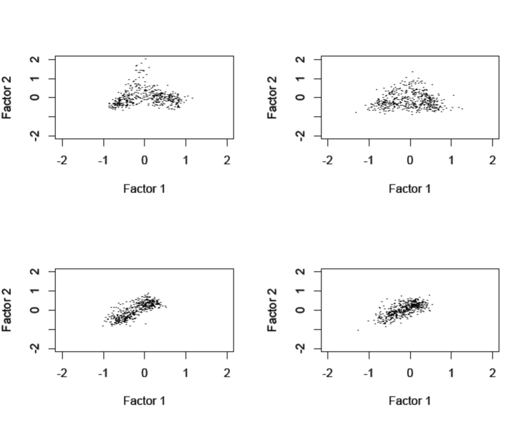
Figure 4: Upper left and right, respectively: the two sets of 500 recipes as used in Figure 3. Lower left and right: these two sets of 500 recipes are projected into the analysis of the 306 recipe collections. What enables this to be accomplished is that the same 1000-word set is used in all cases here.

In Figure 4 we look at the potential for handling massive data sets by projecting into a “primary” analysis. We have this analysis here on the $306\times 1000$ recipe collections times 1000 highest ranked words. We project into the analysis the first $500\times 1000$ recipe set, and the second $500\times 1000$ recipe set.

The scheme used is as follows. We take as a main matrix the one that crosses 306 rows with 1000 columns. Then we have a supplementary row set, of 500 rows crossed with 1000 columns. Finally we have a further supplementary row set, of 500 rows crossed with 1000 columns. The supplementary rows are projected into the Correspondence Analysis of the $306\times 1000$ matrix, post factum.

We note that it is best to carry out the eigen-reduction on the smaller of the row set and the column set. Hence, relative to how we have presented our processing steps above, in fact we worked on the transposed matrices. (For the $306\times 1000$ matrix, diagonalization is carried out on a $306\times 306$ matrix.)

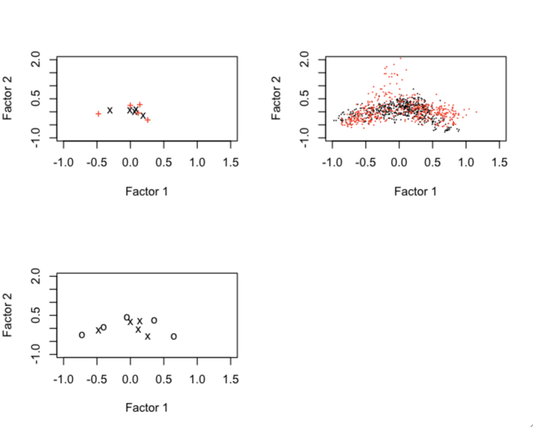
Figure 5: Upper left: red “+” are principal factor plane projections of the 5 recipe-sets, in the $5\times 1000$ dataset, and black “x” are the projections, relative to principal factor plane projection of using the original $500\times 1000$ data. Upper right: a black dot, “.”, represents projections as supplementary elements of the 500 recipes, relative to the derived 5 recipe-sets; and a red dot, “.”, represents the active Correspondence Analysis of these $500\times 1000$ data. So the black dots are efficiently determined, but the red dots show the “ground truth”. Lower panel: different set of 5 recipe-collections, as used previously (e.g. upper left panel here), and then independently defined in order to enhance having “like with like” in the same recipe-collection. Note that in all cases we are using a 2-dimensional (albeit optimal) display.

In Figure 5, in the upper left we show with “x” (i) the projection as supplementary elements of a $5\times 1000$ set of data derived from a $500\times 1000$ set of data; and shown with a red “+” (ii) the projections of the active Correspondence Analysis of the $5\times 1000$ set of data.

The $500\times 1000$ set of data was the set of 500 recipes used before – in fact the sequentially first of these batches of recipes (and as indicated there were 306 of these batches). The word set is 1000, being the top-ranked words in the entire word-set derived from all recipes. From the $500\times 1000$ set of data, we took the first 100 recipes, then recipes 201–300, 301–400, and 401–500. We aggregated the recipes, which is equivalent to concatenating the recipes. This provided a frequency of occurrence cross-tabulation of $5\times 1000$.

In Figure 5, upper right, we show with a dot, “.”, (i) the 500 recipes with their projections found from using the $500\times 1000$ data as supplementary elements relative to the $5\times 1000$ data. We show also, using red dots, “.”, (ii) the active Correspondence Analysis of the $500\times 1000$ data.

In Figure 5, lower panel, there is, with an “x”, (i) the projections of the active Correspondence Analysis of the $5\times 1000$ set of data, as in the upper left. Then, with a “o”, there is (ii) the same analysis on a matrix of the same dimensions, but this time with the 5 concatenated sets of recipes being based not on the given sequential order, but rather on the first factor projections of the full $500\times 1000$ matrix. This was done in order to assess a different derived frequency of occurrence set of data.

Arising out of this discussion, we will draw a balance sheet on projections, through assessment of similarity of outcomes. We use the sums of squared Euclidean distances, taken from the principal plane factor projections, which are Euclidean.

Quality of results based on sum of squared Euclidean distances.

1. Concatenated recipes projected onto full recipe set, versus concatenated recipes: $5\times 1000$ projected onto $500\times 1000$, and active analysis of $5\times 1000$: 0.03306077

2. Full recipe set projected onto concatenated recipes, versus full recipe set: $500\times 1000$ projected onto $5\times 1000$, and active analysis of $500\times 1000$: 0.283562

Next, $5\times 1000$ is “ordered” i.e. based on a chosen sequencing and not an arbitrarily given one. The chosen sequencing is that of projections on the first factor. So, in the foregoing experiment, the 5 groups of recipes, each of 100 recipes, had their sets of 100 recipes in the given, arbitrary, sequence. Now, the 5 groups of recipes, each of 100 recipes, have their sets of 100 recipes in a somewhat clustered sequence that is provided by these recipes’ projections on the first factor.

1. Concatenated clustered recipes projected onto full recipe set, versus concatenated clustered recipes: $5\times 1000$ projected onto $500\times 1000$, and active analysis of $5\times 1000$: 0.9963667

2. Full recipe set projected onto concatenated clustered recipes, versus full recipe set: $500\times 1000$ projected onto $5\times 1000$, and active analysis of $500\times 1000$: 1.097960

What is noteworthy here is that the “ordered”, i.e. somewhat more clustered 100-strong recipe-sets, preform less well than arbitrarily-given 100-strong recipe sets. (Cf. latter two results above vis-à-vis the former two.) We draw the conclusion that the lesser coherence associated with the latter is better when it comes to projecting other recipes into this space.

We see a certain parallel between this outcome and the importance of incoherence in compressed sampling in signal processing. Such incoherence is when [17] (p. 278), there should be as much spread as possible between the sensing vector, on the one hand, and on the other hand, the “sparsity atoms” or basic components that we can use for the signal to be acquired.

We also have an indication from the above that the bigger the better the analysis, in terms of observations, when it is a matter of projecting into the factor space. (Cf. first result above, out of the four, being better than the second result.)

We conclude: the bigger the set of observations that we can work on, so much the better. Also if we do need to work on a limited, representative set of aggregates, then lack of coherence (i.e. lack of clustering) is best.

2.3 The Practical Benefit of a Selected Word Set

We use again the first 500-recipe set. With the word set, as before, derived from the entire set of recipes, we look at (i) the top ranked (i.e. most frequently occurring) 1000 words, (ii) the 42,052 word list such that word lengths are greater than 2, and (iii) the full word set, with 101,060 words. In each case, we therefore used the 500 recipes cross-tabulated with the words in terms of frequency of occurrences. Recall again that the word list used was derived from the entire set of recipes (and not just these 500).

Figures 6 and 7 portray the rapid falloff in inherent embedding dimensionality, based on the word set, and associated attribute dimensionality.

In Figure 6, the (effectively superimposed) 42,052 and 101,060 word sets are on top, and the 1000 word set on the bottom. The reason for the two top curves being superimposed is the following. The full word set is just the words that occur twice or once in the recipes. Hence they are very rare words. Hence, too, while the 500 recipes here are characterized by, on the one hand, 42,052 words, and on the other hand, 101,060 words, nonetheless the extra data is extremely sparse – consisting mostly of zero values. It is small wonder therefore that these two datasets, relating to words with more than two occurrences, and all words, give practically the same outcome.

The top 8 actual eigenvalues are as follows, if we choose, on the basis of Figure 6 to select, e.g. 8 factors as bearing the most important information:

xx1c$evals[1:8]
[1] 0.3441775 0.2973126 0.2854613 0.2463559 0.2445217 0.2348758
    0.2255849 0.2212731
x1c$evals[1:8]
[1] 0.2722012 0.1816320 0.1526613 0.1341513 0.1278123 0.1133759
    0.1084320 0.1009735

Our preference is to focus our interest on just the first three factors, given these eigenvalues.

Figure 6: Eigenvalues from Correspondence Analyses of a set of 500 recipes (the very first of the 306 recipe-sets). Top curve – more or less fully superimposed: using 42,052 words and using the entire word set of 101,060 words. Bottom curve: using 1000 words.

Figure 7: Eigenvalues in percentage terms. Cf. Figure 6 displaying the eigenvalues themselves. Here the top curve relates to the set of 1000 words, and the bottom – more or less fully superimposed – curves relate to the 42,052 word set and using the entire word set of 101,060 words.

2.4 Conclusions

In section 1.2, we observed that: In the case of large, or very large, numbers of occurrences of entities, the syntactically correct form will predominate.

In section 2.2, we concluded that: The bigger the set of observations that we can work on, so much the better. Also if we do need to work on a limited, representative set of aggregates, then lack of coherence (i.e. lack of clustering) is best.

Finally, in section 2.3, we concluded that: Large, sparse word sets lead to a similar outcome; and a well selected, smaller sized word set is important for best, i.e. smallest, reduced dimensionality mapping.

Part 2: Data Analysis of Recipes: Contrasting Analytics using Apache Solr and Correspondence Analysis in R

3 About the Data; followed by Correspondence Analysis of All Recipes using a 247 Word Set

The 152,998 recipes were found to have 101,060 unique words of 1 character or longer, having set all upper case to lower case, and having ignored punctuation, numeric and accented characters. The distribution of terms follows a power law (Zipf’s law): the probability of having more than $x$ occurrences per word was found to be approximately $c/x^{-2.3515}$.

In total we have 152,998 recipes. A set of 247 recipe ingredients was assembled. They were chosen from a word list (unique words) drawn from the recipes and ordered by decreasing frequency of occurrence. There were just 122 recipes that did not contain at least one of these 247 ingredient terms. (That could be due to use of less common ingredients, not figuring in our list of 247; or misspellings, of which there were a considerable number; or some unusual text instead of a recipe. An example of the latter was a short overview of appropriate wines for types of food.)

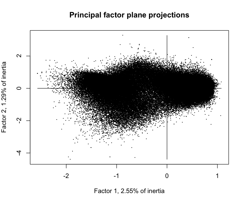
Figure 8: Principal factor plane showing projections of 152,998 recipes, each represented by a dot.

Figure 8 shows the projections of recipes on the principal factor plane.

Figure 9 shows the ingredients used, projected onto the principal factor plane. The ingredients with the strongest contributions to these factors are noted. Looking further, we found that the strongest contribution by ingredients to factor 3 is “chocolate”; and the strongest contribution to factor 4 is “cheese”.

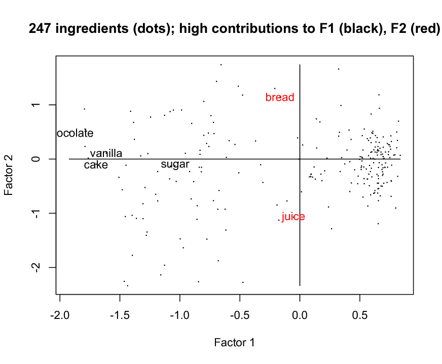
Figure 9: Principal factor plane showing projections of 247 ingredients, using a dot to represent projection. Strongest contributions to factor 1: “sugar”, “chocolate”, and a little less, “vanilla”, “cake”. Strongest contributions to factor 2: “juice”, “bread”.

4 Search using Solr

4.1 Setting Up Data File and Its Description

The Solr (lucence.apache.org/solr) search server was used.

1. The data to be indexed, and supported for search, is put into xml with the following structure:

   • <add> and </add> at beginning and end.

   • Each entry defined by <doc> and </doc>.

   • A required field providing a unique identifier:

     <field name=’’id’’>mm000001102.txt</field>.

   • Other fields, such as the following for bounding box search:

     <field name=’’xcoord’’>-0.7341409</field>

     <field name=’’ycoord’’>-0.09961348</field>

     (Note that these coordinates are the principal factor coordinates resulting from a Correspondence Analysis. I.e., they are the factor 1 and factor 2 projections, respectively.)

   • Other fields such as:

     <field name=’’name’’>’’21’’ Club Rice Pudding</field>

   • The main text field, tagged by: <field name=’’recipe’’>...</field>.

   The xml file was of size over 205.5 MB. It was put in directory example/exampledocs.

2. Two files in directory example/solr/collection1/conf need to be fully cognizant of the xml data to be used. These are schema.xml and solrconfig.xml. In the latter, changes made included the following, with regard to mlt or MLT, “More Like This” option.

   In the requestHandler there is:

          <arr name="components">
            <str>query</str>
            <str>facet</str>
            <str>mlt</str>
            <str>highlight</str>
            <str>stats</str>
            <str>debug</str>
          </arr>
       </requestHandler>
   
   ...
   
          <!-- Query settings -->
          <str name="defType">edismax</str>
          <str name="qf">
             recipe^1.0
          </str>
          <str name="df">text</str>
          <str name="mm">100%</str>
          <str name="q.alt">*:*</str>
          <str name="rows">10</str>
          <str name="fl">*,score</str>
   
          <str name="mlt.qf">
             recipe^1.0
          </str>
          <str name="mlt.fl">recipe</str>
          <!-- Following: no. of nearest neigbours returned in MLT -->
          <int name="mlt.count">1</int>
   
          <!-- Faceting defaults FM CHANGED TO off -->
          <str name="facet">off</str>
   

3. In file schema.xml the fields used and their definitions need to be defined. This included:

   <field name="recipe" type="text_general" indexed="true" stored="true"

   termVectors="true"/>

   Also:

      <field name="xcoord" type="double" indexed="true" stored="true" />
      <field name="ycoord" type="double" indexed="true" stored="true" />
   

4. For the browser-based querying, this is management by the velocity component, that is in subdirectory example/solr/collection1/conf/velocity.

   The files changed there, to be appropriate for the data analyzed, were: browse.vm, footer.vm, header.vm, product-doc.vm, query.vm. Display images (see the principal factor plane in Figures 10, 11) used there are located in the named image directory, which is currently
   example/solr-webapp/webapp/img.

4.2 Running the Server and Updating the Index

The Solr server is started thus, in directory example, where in this example, 1 GB of memory is provided:

java -Xmx1024m -jar start.jar

To update, or commence, indexing, in the directory containing the xml data, example/exampledocs, the following command is issued. This supposes a running server.

java -jar post.jar recipes-F1F2-1.xml

The unique identifier field is the crucial aspect of what gets taken into the index, or updated.

4.3 Querying and Other Operations

4.3.1 Web Browser User Interface

The following access address is used, based on the running server:

http://localhost:8983/solr/browse

Through the upper right hand corner link to the Admin screen, or directly using http://localhost:8983/solr/#/collection1, there is availability of the log file; querying can be carried out; statistics of use and of the data can be accessed. Note that as currently configured in this work, collection1 contains the indexed data.

Example of query: “sugar beer pasta”. A required term is specified in the query with a preceding plus sign, and a requirement not to have a term is specified with a minus sign preceding the term. The “More Like This” option gives a number of nearest neighbours of the document, and its parameters are defined in the settings in schema.xml.

Figures 10 and 11 show examples of use. The Correspondence Analysis figure at the top is static. It and the table to its left are provided as navigation aids in search and discovery. The table to the left of the Correspondence Analysis principal factor plane is also static. An alternative could be a text cloud or cloudmap (see [14]).

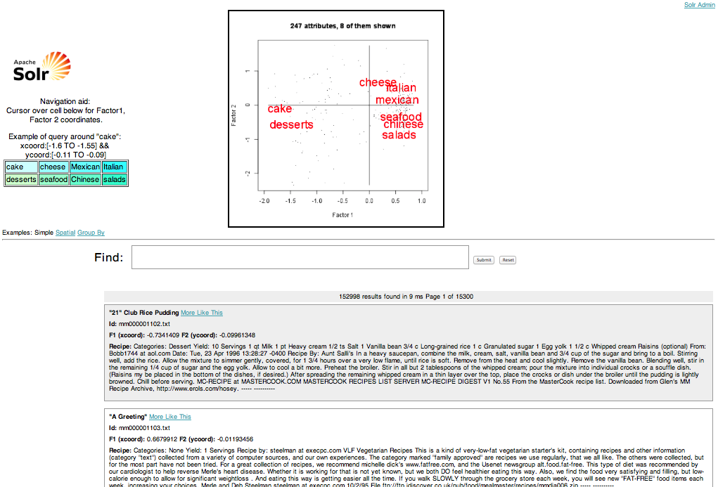
Figure 10: Screenshot of browse Solr window, before submitting a query. For each recipe (and here, to begin with, the 152,998 recipes are listed), the id (identifier), coordinates (factors 1 and 2), are given, followed by the entire recipe which has had new line characters ignored. The “More Like This” option follows the recipe name.

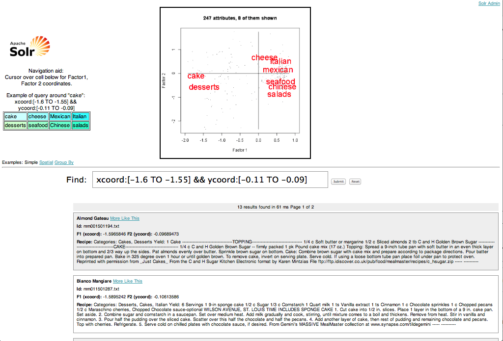
Figure 11: Screenshot (second) of browse Solr window. A bounding box query has been given, based on the coordinates of the attribute “cake”.

4.3.2 Command Line Querying

An example follows (all to be placed on one line). For this, three “More Like This” near neighbours were required (i.e., in file solrconfig.xml, there was this setting: <int name=’’mlt.count’’>3</int>).

curl -o out.xml ’http://localhost:8983/solr/collection1/
      browse?&q=id:mm078001428.txt&wt=xml&mlt=true’

In this case, results are saved to file out.xml. From a search for recipe mm078001428.txt, a “More Like This” request is submitted.

From the file out.xml here is a little utility to write out just the recipe identifiers (all on one line):

awk -v srch="\"id\">" ’BEGIN{l=length(srch)} END{print "\n"}
{t=match($0,srch);if(!t){next}extr=substr($0,t+5,15);printf "%s ", extr}’
< out.xml

In this case, this gives:

mm078001428.txt mm110501451.txt mm158501305.txt mm161501159.txt

5 Consistency of Solr Searches

Using identifier (and recipe) “mm078001428.txt”, with name “No Fat, No Salt, No Sugar Vanilla Ice Cream”, we found its “More Like This” best match to be “mm110501451.txt”, with name “Sugar-Free Cappuccino Ice Cream”. Using the latter, we found its best match to be the former, thereby showing consistency. More specifically, the two recipes in this case were mutual or reflexive nearest neighbours. See [9] for the use of this principle (of mutual nearest neighbours, and also nearest neighbour chains) in agglomerative hierarchical clustering algorithms.

We also sought best match recipes using the Correspondence Analysis factor space. This latter is of course Euclidean. We used the full space dimensionality (hence 247 less 1 due to linear dependence through centring the cloud of recipes, and the dual cloud of ingredients). For recipe “mm078001428.txt”, we got its closest neighbour as “mm048501554.txt”, “Fruit Flavor Milk Shakes”. For recipe “mm110501451.txt”, we got its closest neighbour as “mm161501159.txt”, “Vanilla Ice Cream - Diabetic *WW No.2”

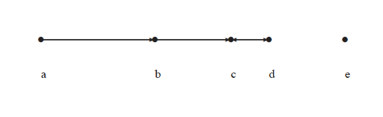
Figure 12: Nearest neighbours. Point $b$ is the nearest neighbour of point $a$. Point $c$ is the nearest neighbour of point $b$. Point $d$ is the nearest neighbour of point $c$, and reciprocally $c$ is the nearest neighbour of point $d$.

In Figure 12 the geometric situation is depicted, irrespective of how nearest neighbour is defined (it need not be a distance but some dissimilarity satisfying $d(a,b)=0\mbox{ if }a=b$; $d(a,b)\geq 0$; and the closer $a$ is to $b$, i.e. the more alike they are, the smaller the value of $d(a,b)$).

The squared Euclidean distance in the full dimensional Euclidean factor space gives for the pair of best match recipes furnished by Solr, 18.94413. Then in the full dimensional factor space, the best match distance squared of “mm078001428.txt”, as noted above, was 4.934411; and the best match distance squared of “mm110501451.txt” was 6.103886. To note that the Correspondence Analysis best match distances are supported by the data is to be unfair to what is, with Solr, a different framework for determining best matches. This includes using all words, with stemming and lemmatization, compared to the 247 ingredients used in the Correspondence Analysis case.

We note that the Solr best match information lends itself to looking for clusters such that nearest neighbour chains are followed, and once a (mutual or reciprocal) nearest neighbour pair is found, they can be agglomerated with no impact on close-by recipes. This is due to Bruynooghe’s reducibility property. Background on nearest neighbour chain, and reciprocal nearest neighbour based hierarchical agglomerative clustering can be found in [9].

Appendix 1: Sample Recipe

Recipe mm160001 collection, number 245 out of 500 in sequence from this collection, is as follows.

      Title: The Perfect Roast Chicken with Roasted Shallots And Portob
 Categories: Lifetime tv, Life5
      Yield: 4 servings

      4 lb Young roaster
           Salt and pepper; to taste
      1 md Onion; halved and peeled
      3    Cloves garlic; peeled and
           -smashed
      1 bn Fresh herbs; rosemary thyme
           ; flat-leaf parsley
    1/4 c  Olive oil
      2 c  Chicken broth; divided
      8 lg Shallots
      8    Portobello mushrooms; stems
           -removed and
           ; cut in half
    1/2 c  Dry white wine

  How to Prepare the Chicken:

  1. Preheat the oven to 350 F. Season the skin and the inside of the cavity
  of the chicken generously with salt and pepper.

  2. Place the onion, garlic, and fresh herbs in the cavity and truss the
  chicken. In a roasting pan over medium-high heat, heat the oil until it
  begins to smoke.

  3. Place the chicken, breast-side-down, in the oil and cook until all the
  sides off the chicken are completely browned.

  4. Place the bird, breast-side-up into the oven and baste with 1/4 cup of
  the chicken stock. Continue basting with 3/4 cup of the chicken stock every
  10 minutes until the chicken is done, approximately 1 hour, or until the
  chicken reaches an internal temperature of 170 F.

  5. Add the shallots 20 minutes after the chicken has been put into the oven
  and the mushrooms 40 minutes after the chicken has been put into the oven.

  6. Remove the cooked chicken, shallots, and mushrooms from the oven and set
  on a platter, cover and let rest for 10 minutes.

  How to Prepare the Sauce:

  1. Place the roasting pan back on the stove over medium-high heat and bring
  the juices in the pan to a boil. Using a small ladle remove any of the fat
  that has risen to the top of the pan.

  2. Add the white wine to the pan and, using a wooden spoon, scrape up the
  browned bits from the bottom of the pan. Reduce the wine by half and add
  the remaining 1 cup of chicken stock.

  3. Reduce the stock by half, season with salt and pepper and add the fresh
  thyme. Carve the chicken and arrange on a platter with the shallots and
  mushrooms. Spoon the pan juices over the meat.

  The Perfect Roast Chicken With Roasted Shallots and Portobello

  <A9> 1997 Lifetime Entertainment Services. All rights reserved.

  MC formatted using MC Buster by Barb at PK

    Converted by MM_Buster v2.0l.

-----

We note the following in this recipe text: Abbreviations (“lg”, large; “lb”, pounds; “c”, cup; etc.). Source and other summarized or abbreviated data. A control character (“$<$A9$>$”).

Appendix 2: 247 Ingredients Used as Attributes in the Correspondence Analysis

List of 247 ingredients used, with their frequencies of occurrence.

          salt          sugar          water         pepper            oil         butter
        167636         142624         134454         132012         126242         115387
         sauce          flour         garlic          cream         cheese        chicken
        105909          99870          85080          83859          80835          78635
         onion          juice            egg           milk          lemon           eggs
         73933          65773          62000          61125          55408          50086
         bread         onions           rice      chocolate          olive        vanilla
         48789          44169          41645          40737          39539          38386
          cake       tomatoes        parsley       potatoes        vinegar      vegetable
         35317          34894          32217          31423          31340          30735
          wine         tomato          beans           beef     vegetables         cloves
         29192          28747          28180          28761          27203          27034
          soup         orange       cinnamon      margarine      mushrooms          salad
         26558          25976          25656          24266          23693          23612
          fish           corn          broth         celery        mustard            pie
         23267          21212          20832          21193          20192          20081
         pasta          fruit        peppers            soy          chili          basil
         19743          18989          18695          18036          17148          16354
        shrimp           soda        cookies          syrup        carrots          honey
         16332          16257          16216          15652          15197          14733
        sodium         cookie       parmesan            ice       dressing     cornstarch
         14034          14173          13878          13928          13886          13848
         thyme          bacon         pastry           lime          yeast         potato
         13636          13653          13309          13274          13347          12957
         apple        protein        spinach      casserole        oregano          cumin
         12642          12129          11889          12106          11855          11996
        nutmeg    cholesterol        raisins          clove        coconut      pineapple
         11756          11376          11019          11042          10892          10864
         roast          chips           chop          puree        topping       marinade
         10758          10667          10637          10638          10542          10586
       noodles           loaf       desserts       cilantro          yolks         peanut
         10441          10456          10371          10405          10362          10258
       italian          chile      seasoning         apples        almonds           peas
         10285          10293          10350          10280          10216          10459
        sesame         turkey            ham        cabbage        paprika           leaf
         10184           9975           9725           9736           9689           9703
         mixer         yogurt      coriander   carbohydrate        sausage        cayenne
          9211           9067           8903           8765           8918           8892
          lamb          wheat           bean        walnuts          cakes           mint
          8571           8639           8573           8470           8398           8256
       lettuce     mayonnaise         pecans         sherry          cocoa        pudding
          8159           8000           7893           7950           7835           7843
       cheddar          grain         salmon         olives         carrot          shell
          7877           7806           7724           7744           7767           7511
    vegetarian       broccoli       zucchini          salsa         flakes         grease
          7405           7413           7290           7268           7104           7079
       chinese       shallots        poultry       mushroom          steak       rosemary
          7079           6877           6969           6857           6927           6699
      eggplant         chiles           rind          curry         coffee           dill
          6708           6804           6696           6798           6602           6683
        spices         breads     buttermilk worcestershire         starch        seafood
          6648           6670           6351           6273           6031           6135
       pumpkin        gelatin  carbohydrates      scallions         almond         chives
          5820           5899           5749           5815           5662           5621
         spice          meats          herbs           tofu        dessert          pizza
          5576           5591           5496           5409           5466           5398
  strawberries         juices        muffins        mexican      tortillas          chops
          5373           5318           5290           5176           5139           4996
           rum          icing          soups       cornmeal         emeril      asparagus
          5014           4917           5084           5032           4874           4740
        sauces         muffin         fruits       stuffing          jelly         salads
          4792           4778           4737           4704           4756           4731
        shells       jalapeno     mozzarella         banana         steaks         greens
          4645           4581           4484           4387           4354           4390
     spaghetti        broiler       cucumber       cherries          toast         cherry
          4343           4346           4679           4351           4307           4358
       chilies           yolk          gravy          cider           root        tabasco
          4324           4289           4258           4244           4304           4272
          oats          fiber           veal       tortilla           sage          dijon
          4225           4135           4061           4085           4040           4040
       bananas          broil           tuna       molasses        peaches    peppercorns
          3970           3970           3914           3949           3939           3928
         candy           duck       tarragon         fennel           tart        custard
          3884           3805           3851           3789           3814           3774
         maple       scallops           stew         brandy        berries          pears
          3749           3871           3802           3780           3777           3559
          crab  confectioners       crackers       biscuits       bouillon        peanuts
          3611           3571           3570           3464           3526           3440
         leeks           beer       turmeric         stalks        ricotta        oranges
          3392           3450           3385           3393           3274           3278
       lentils      raspberry        cracker           herb    raspberries     strawberry
          3260           3216           3128           3113           3083           3093
           jam
          3151

Appendix 3: Alternative Presentation of Plot

Figure 13 shows an improved presentation of Figure 9, through movement of projections (from the red dots, indicated by the stick lines), as implemented in the textplot program in the Word Cloud package in R [3].

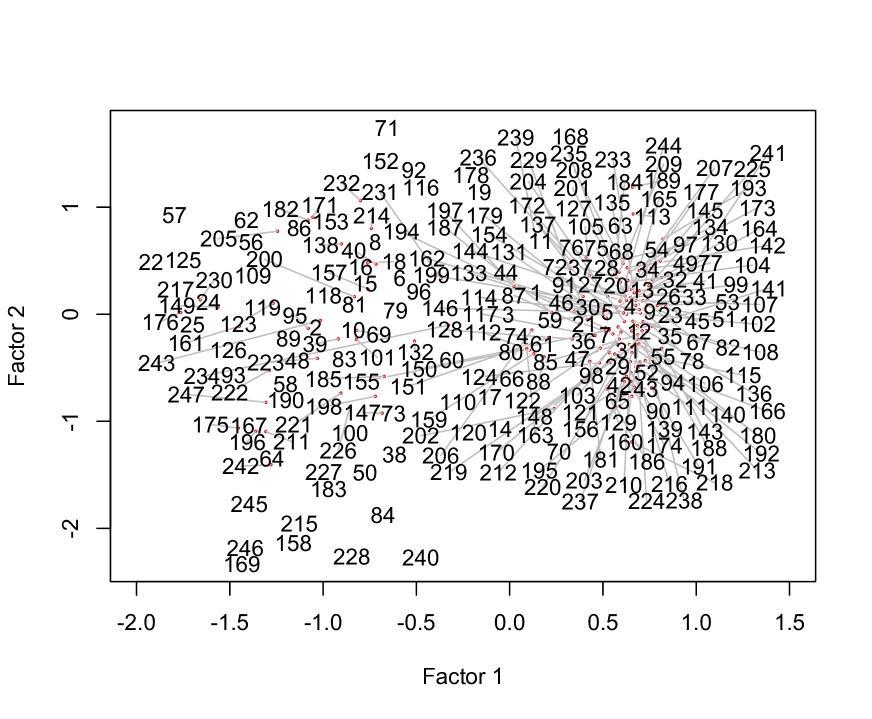
Figure 13: Principal factor plane showing projections of 152,998 recipes, each represented by a dot.

6 Appendix 4: Correspondence Analysis for Singular/Plural Association and Potentially for Disambiguation

In the recipe set, there were 101,060 unique words. Words were as defined by us: length $\geq 1$; all upper case set to lower case; punctuation removed; numeric and accented characters ignored. Variations on spelling included the following example, with numbers of occurrence in the recipe set:

zucchini 7155
zuchinni 86
zuccini 57
zucchinis 56
zuchini 40
zucchine 14
zucchinni 7
zucchin 6
zuckinni 5
zuchinnis 4
zuccinni 3
zuccchini 2
zuccihini 2
zuchhini 2
azucchini 1
brushingzucchini 1
lambzucchini 1
ofzucchini 1
pzucchini 1
zucchiniabout 1
zucchinii 1
zucchinnis 1
zucchni 1
zucchnini 1
zuccinis 1
zuchhinis 1
zuchine 1
zuchinis 1
zucinni 1
zzzucchini 1

On this list we see some words run together, singulars and plurals, but also all manner of misspellings.

We examine here, using the 152,998 $\times$ 247 ingredients set, the projections in the principal factor plane of singulars and plurals. Recall that the principal factor plane, while being the best visualization of the data, with inherent dimensionality 246, only accounts for just over 3.8% of the total inertia.

The singulars used were as follows, with additionally their 23 corresponding plurals: “strawberry”, “carrot”, “muffin”, “egg”, “apple”, “yolk”, “tortilla”, “bread”, “cookie”, “pepper”, “juice”, “vegetable”, “clove”, “carbohydrate”, “spice”, “soup”, “peanut”, “onion”, “olive”, “cracker”, “almond”, “bean”, “banana”.

Figure 14: Principal factor plane showing projections of 247 ingredients, using a dot to represent projection, together with 23 singulars of ingredient names. Cf. Figure 15 for the corresponding plurals of these names.

Figure 15: Principal factor plane showing projections of 247 ingredients, using a dot to represent projection, together with 23 plurals of ingredient names. Cf. Figure 14.

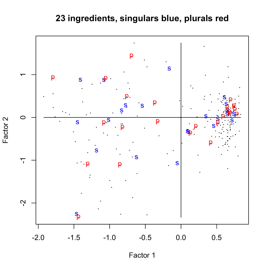
Figure 16: Combining Figures 14 and 15, this shows 23 singulars (“s”) and plurals (“p”).

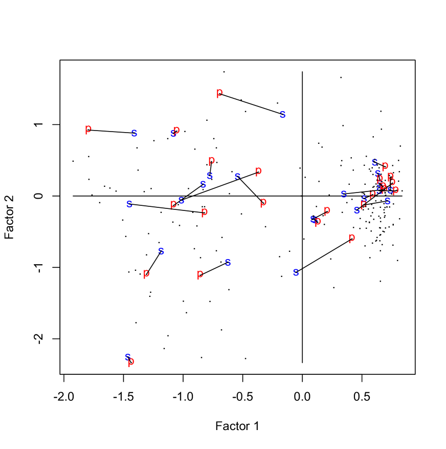
Figure 17: Links shown for all singular and plural pairs.

Figures 14, 15, and also 16 with links drawn for all singular and plural pairs, show the close association in the principal factor plane. Some singulars and plurals are admittedly somewhat separated, e.g. “cracker”, “yolk”, pointing to some difference in semantic – clearly possible in practice – and contextual use of singular and plural. Overall the association between the terms is well exemplified in the figures.

References

- [1] S. Deerwester, G.W. Dumais, S.T. Furnas, T.K. Landauer and R. Harshman, “Indexing by latent semantic analysis”, Journal of the American Society for Information Science, 41, 391–407, 1990.
- [2] N. Eiron and K.S. McCurley, “Link structure of hierarchical information networks”, Proc. Third Workshop on Algorithms and Models for the Web-Graph (WAW 2004), Lecture Notes in Computer Science, pp. 143–155, 2004.
- [3] I. Fellows, Word Clouds, software in R written by Ian Fellows, version 2.2, 2012-09-05, http://log.fellstat.com/?cat=11
- [4] P. Hall, J.S. Marron and A. Neeman, “Geometric representation of high dimension, low sample size data”, Journal of the Royal Statistical Society B, 67, 427–444, 2005.
- [5] B. Le Roux and H. Rouanet, Geometric Data Analysis, Kluwer, 2004.
- [6] B. Le Roux and H. Rouanet, Multiple Correspondence Analysis, Sage, 2010.
- [7] M. Mitzenmacher, “A brief history of generative models for power law and lognormal distributions”, Internet Mathematics, 1, 226–251, 2004.
- [8] A. Morin, “Interactive text mining and applications”, NTTS 2011 – New Techniques and Technologies for Statistics 2011, presentation (78 pp.) at http://www.cros-portal.eu/book/export/html/17
- [9] F. Murtagh, Multidimensional Clustering Algorithms, Physica-Verlag, 1985.
- [10] F. Murtagh and A. Heck, Multivariate Data Analysis, Kluwer, 1987.
- [11] F. Murtagh, “On ultrametricity, data coding, and computation”, Journal of Classification, 21, 167–184, 2004.
- [12] F. Murtagh, “Identifying the ultrametricity of time series”, European Physical Journal B, 43, 573–579, 2005.
- [13] F. Murtagh, Correspondence Analysis and Data Coding with R and Java, Chapman & Hall/CRC, 2005.
- [14] F. Murtagh, A. Ganz, S. McKie, J. Mothe and K. Englmeier, “Tag Clouds for Displaying Semantics: The Case of Filmscripts”, Information Visualization Journal, 9, 253-262, 2010.
- [15] E. Neuwirth and L. Reisinger, “Dissimilarity and distance coefficients in automation-supported thesauri”, Information Systems, 7, 47–52, 1982.
- [16] M.E.J. Newman, “The structure and function of complex networks”, SIAM Review, 45, 167–256, 2003.
- [17] J.-L. Starck, F. Murtagh and J. Fadili, Sparse Image and Signal Processing: Wavelets, Curvelets, Morphological Diversity, Cambridge University Press, 2010. (2nd edition forthcoming 2015.)