2.4cm2.4cm2cm2cm

It is known that the Yangian of $PSU(2,2|4)$ is a symmetry of the tree-level $S$-matrix of $\mathcal{N}=4$ super Yang-Mills. On the other hand, the complete one-loop dilatation operator in the same theory commutes with the level-one Yangian generators only up to certain boundary terms found by Dolan, Nappi and Witten. Using a result by Zwiebel, we show how the Yangian symmetry of the tree-level $S$-matrix of $\mathcal{N}=4$ super Yang-Mills implies precisely the Yangian invariance, up to boundary terms, of the one-loop dilatation operator.

1 Introduction

The study of ${\cal N}=4$ supersymmetric Yang-Mills (SYM) theory has been dominated by two broad strands of research – the first concentrating on the anomalous dimensions of local operators (i.e. the spectral problem) and their correlation functions, and the second investigating the scattering amplitudes of the theory. The successes in these two areas have been considerable in their own right, and at the current time there is vigorous activity focussing on making connections between them in order to deepen our understanding of this fascinating quantum field theory.

In the planar limit the spectral problem is believed to be integrable. This was first shown at one loop in [1] for a particular sector of the theory. The complete one-loop dilatation operator was later computed in [2], following earlier results in [3], and later shown in [4] to describe a $PSU(2,2|4)$ super spin chain. The one-loop dilatation operator is invariant under the (free) superconformal symmetry, and in fact this condition puts strong constraints on its form.

One of the key features of integrability is the existence of an infinite hierarchy of non-local charges $Q^{A}$ built upon the basic local (or level-zero) $PSU(2,2|4)$ Noether charges $J^{A}$ of the theory. These non-local charges, together with the local ones, obey a Yangian algebra which in the context of the one-loop dilatation operator $H$ was described in [5]. Interestingly, it was found in that paper that $H$ commutes with these additional non-local charges up to certain boundary terms,

$$[Q^{A},H]\sim J^{A}_{1}-J^{A}_{L}\ ,$$ (1.1)

where $L$ denotes the length of the chain (or number of fields in the operator). One intriguing aspect of this relation, which we will return to later, is that it mixes tree-level and one-loop quantities [6].

The study of scattering amplitudes in ${\cal N}=4$ SYM started off independently from considerations of integrability, but has recently begun to be connected to it in various ways. An important discovery was that of dual superconformal symmetry of the ${\cal N}=4$ SYM $S$-matrix. This was conjectured in [7] and tested in several cases, and shortly after proved at tree level in [8]. At one loop the symmetry is broken because of the presence of infrared divergences in the amplitudes, and the breaking is controlled by a dual conformal Ward identity proposed in [9] and confirmed with a direct amplitude calculation at one loop in [10]. Importantly, in [11] the standard and dual superconformal symmetries were embedded into the Yangian of $PSU(2,2|4)$. Explicit expressions of the level-one generators were constructed and shown to be related to the generators of the dual superconformal algebra. At tree level the symmetry is slightly broken [12] due to collinear singularities of the amplitudes, leading to anomalies that are supported only on special kinematic configurations. As mentioned earlier, at one loop infrared divergences lead to additional anomalies. Interestingly, these violations can be absorbed into appropriate redefinitions of the Yangian generators both at tree level [12] and one loop [13].

The presence of a Yangian symmetry on the dilatation operator and the amplitude sides makes one naturally think that these symmetries are the manifestation of a single underlying Yangian symmetry of the theory. However these two symmetries are seemingly realised in a different manner, given (1.1) and the fact that on the amplitude side, the symmetry can be realised exactly, with the Yangian generators annihilating the amplitudes (divided by the MHV part). The goal of this paper is that of reconciling these two situations by finding a proof of (1.1) which relies on the Yangian symmetry of the tree-level $S$-matrix of ${\cal N}=4$ SYM, therefore substantiating the connection between the Yangians of the spin chain and the amplitudes.

A direct connection between the one-loop nearest-neighbour part of the spin-chain dilatation operator and amplitudes, which will be very relevant for our investigation, was found in [14] by Zwiebel, working off of an earlier observation of Beisert. In that paper the one-loop dilatation operator, expressed in the so-called “harmonic action” form [2], was related to the integration of a four-point superamplitude glued to a tree-level form-factor with two external legs over the two-particle phase space, see Figure 1.

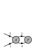
Figure 1: In [14] it was shown that the harmonic action (2.5) is recovered via the sewing together of a tree-level four-point superamplitude ${A}$ and a tree-level form factor ${P}$ corresponding to the particular two-site spin-chain state under consideration.

In [15], this connection was explained in terms of one-loop form factors of generic operators. Specifically, it was shown there that the result of [14] is the coefficient of the discontinuity of a bubble integral associated with this one-loop form factor, and captures the ultraviolet-divergent part of the calculation.

In the following we will use Zwiebel’s formula to show that the invariance of the amplitudes under the Yangian, and certain special properties of the Yangian of $PSU(2,2|4)$, lead precisely to the expected result (1.1).

The plan of the paper is as follows. In section 2 we review basic facts about the one-loop dilatation operator and its various realisations. Furthermore, we review the Dolan-Nappi-Witten [5] proof of (1.1), which relies on a special set of eigenstates and motivate the calculation of the commutator $[Q,H]$. In section 3 we present a novel proof using ideas from amplitudes that does not rely on any choice of a basis of states.

2 Review and motivation

In this section we review some important facts about the dilatation operator and Yangian symmetry. We will then motivate the calculation of the commutator $[Q,H]$ performed in the next section using the representation of the dilatation operator in terms of amplitudes and form factors found in [14].

2.1 States and the spinor-helicity formalism

We consider single-trace local operators in ${\cal N}=4$ SYM of the form ${\rm Tr}(\Phi_{1}\cdots\Phi_{L})(x)$, where the letters $\Phi$ are taken from the list $F^{\alpha\beta},\ \psi^{\alpha ABC},\ \phi^{[AB]},\ \bar{\psi}^{\dot{\alpha}A},\ \bar{F}^{\dot{\alpha}\dot{\beta}}$ (and symmetrised covariant derivatives acting on them), where $A=1,\ldots,4$ is a fundamental $SU(4)$ index.

It is well known [22] that the operators can be described in terms of excitations of two pairs of bosonic oscillators and one pair of fermionic oscillators, satisfying

$$[a_{\alpha},a^{\dagger\beta}]=\delta_{\alpha}^{\beta}\,,\quad[b_{\dot{\alpha}},b^{\dagger{\dot{\beta}}}]=\delta_{\dot{\alpha}}^{\dot{\beta}}\,,\quad\{d_{A},d^{\dagger B}\}=\delta_{A}^{B}\,,\quad\alpha,\beta=1,2,\ \dot{\alpha},\dot{\beta}=1,2,\ A=1,\ldots,4,$$ (2.1)

where the map to the letters introduced above is

$$\bar{F}\leftrightarrow b^{\dagger}b^{\dagger}\,,\quad\bar{\psi}\leftrightarrow b^{\dagger}d^{\dagger}\,,\quad\phi\leftrightarrow d^{\dagger}d^{\dagger}\,,\quad\psi\leftrightarrow a^{\dagger}d^{\dagger}d^{\dagger}d^{\dagger}\,,\quad F\leftrightarrow a^{\dagger}a^{\dagger}d^{\dagger}d^{\dagger}d^{\dagger}d^{\dagger}\ ,$$ (2.2)

while for derivatives $D\leftrightarrow a^{\dagger}b^{\dagger}$. For instance, the Konishi operator $K=\epsilon_{ABCD}\phi^{AB}\phi^{CD}$ is represented as $\epsilon_{ABCD}d^{\dagger A}_{1}d^{\dagger B}_{1}d^{\dagger C}_{2}d^{\dagger D}_{2}|0\rangle$.

The commutation relations (2.1) can then be realised in terms of spinor-helicity variables, commonly used to describe amplitudes. The map in this case is

$$\begin{split}a^{\dagger\alpha}&\leftrightarrow\,\lambda^{\alpha}\,,\quad b^{\dagger\dot{\alpha}}\leftrightarrow\,\tilde{\lambda}^{\dot{\alpha}},\quad d^{\dagger A}\leftrightarrow\,\eta^{A}\,\\ a_{\alpha}&\leftrightarrow\,{\partial\over\partial\lambda^{\alpha}}\,,\ \,b_{\dot{\alpha}}\leftrightarrow\,\frac{\partial}{\partial\tilde{\lambda}^{\dot{\alpha}}},\,\,\,d_{A}\leftrightarrow\,\frac{\partial}{\partial\eta^{A}}\,,\end{split}$$ (2.3)

and, as usual in ${\cal N}=4$ SYM, we combine the $\lambda$, $\tilde{\lambda}$ and $\eta$ variables into a single object $\Lambda^{a}:=\big{(}\lambda^{\alpha},\tilde{\lambda}^{\dot{\alpha}},\eta^{A}\big{)}$. In this formalism, a state is simply a polynomial in the $\Lambda$’s satisfying the physical state condition of vanishing central charge at each spin-chain site, i.e. it has a sensible translation back to the letters $F^{\alpha\beta},\ \psi^{\alpha ABC},\ \phi^{[AB]},\ \bar{\psi}^{\dot{\alpha}A},\ \bar{F}^{\dot{\alpha}\dot{\beta}}$ (and symmetrised covariant derivatives acting on them), and we denote it as $P(\Lambda_{1},\dots,\Lambda_{L})$. Again, the Konishi operator is represented in this language as $\epsilon_{ABCD}(\eta^{A}_{1}\eta^{B}_{1})(\eta^{C}_{2}\eta^{D}_{2})$. We also note that in [15] it was observed that $P(\Lambda_{1},\dots,\Lambda_{L})$ is nothing but the minimal form factor of the operator represented by the state via the dictionaries (2.2) and (2.3).

2.2 The complete one-loop dilatation operator

At one loop and in the planar limit only two neighbouring fields interact, and the one-loop dilatation operator $H$ is the sum of densities $H_{ii+1}$, i.e. $H=\sum_{i=1}^{L}H_{ii+1}$, where $L$ is the number of fields in the operator (or sites in the spin chain, of which $H$ is the Hamiltonian), and $H_{ii+1}$ acts only on fields at position $i$ and $i+1$. The complete one-loop dilatation operator was derived in [2], with the result

$$H_{12}\ =\ \sum_{j=0}^{\infty}2h(j)\,\mathbb{P}_{12,j}\ .$$ (2.4)

Here $h(j)$ is the $j^{\rm th}$ harmonic number and $\mathbb{P}_{12,j}$ projects onto a two-particle state with total spin $j$. The same paper also introduced an alternative representation of the dilatation operator in terms of the oscillators introduced in (2.1) termed “harmonic action”. It is this representation which will be particularly relevant for us, and specifically a rewriting of the harmonic action in an integral form which was found in [24]. Written in terms of spinor-helicity variables the action is:

$$H_{12}\,P\big{(}{\Lambda}_{1},{\Lambda}_{2}\big{)}\ =\ -{1\over\pi}\int_{0}^{2\pi}\!d\phi\int_{0}^{\pi\over 2}\!d\theta\,\cot\theta\Big{[}e^{2i\phi}P\big{(}{\Lambda^{\prime}}_{1},{\Lambda^{\prime}}_{2}\big{)}\,-\,P\big{(}{\Lambda}_{1},{\Lambda}_{2}\big{)}\Big{]}\ .$$ (2.5)

Here by $P(\Lambda_{1},\Lambda_{2})$ we mean $P(\cdots,\Lambda_{1},\Lambda_{2},\cdots)$ where the dots stand for all other fields in the state represented by $P$ that are not involved in the interaction. Moreover the $\Lambda^{\prime}$’s represent “rotated” spinor-helicity variables defined as

$$\left(\begin{array}[]{c}\lambda^{\prime}_{1}\\ \lambda_{2}^{\prime}\end{array}\right):=\mathcal{U}\left(\begin{array}[]{c}\lambda_{1}\\ \lambda_{2}\end{array}\right)\,,\quad\left(\begin{array}[]{c}{\tilde{\lambda}}_{1}^{\prime}\\ {\tilde{\lambda}}_{2}^{\prime}\end{array}\right):=\mathcal{U}^{\ast}\left(\begin{array}[]{c}{\tilde{\lambda}}_{1}\\ {\tilde{\lambda}}_{2}\end{array}\right)\,,\left(\begin{array}[]{c}\eta_{1}^{\prime}\\ \eta_{2}^{\prime}\end{array}\right):=\mathcal{U}^{\ast}\left(\begin{array}[]{c}\eta_{1}\\ \eta_{2}\end{array}\right)\,,$$ (2.6)

with the matrix $\mathcal{U}$ given by

$$\mathcal{U}:=\left(\begin{array}[]{cc}\cos\theta&-e^{i\phi}\sin\theta\\ \sin\theta&e^{i\phi}\cos\theta\end{array}\right)\ .$$ (2.7)

Note that while the state $P$ satisfies the central charge condition, the rotated state in general violates this. The integration over $\phi$ in (2.5) is precisely enforcing the condition that the action of $H_{12}$ on $P$ returns a physical state.

2.3 Connection to form factors

As a final ingredient, we review an alternative form of (2.5) that was also discussed in [14]. This representation for the action of the one-loop dilatation operator on a state $|1,2\rangle$ has the form

$$H_{12}|1,2\rangle\ =\ \int\!d\Lambda\ A(1,2,3,4)\big{[}P(-4,-3)\,-\,r\,P(1,2)\big{]}\ ,$$ (2.8)

where momentum conservation reads $p_{1}+p_{2}+p_{3}+p_{4}=0$. $p_{1}$ and $p_{2}$ are the external legs, while $p_{3}$ and $p_{4}$ are integrated over with the appropriate two-particle phase-space measure

$$d\Lambda=\prod_{i=3}^{4}d^{2}\lambda_{i}d^{2}\tilde{\lambda}_{i}d^{4}\eta_{i}\ .$$ (2.9)

Note that

$$A(1,2,3,4)=\frac{\delta^{(4)}(p)\,\delta^{(8)}(q)}{\langle 12\rangle\langle 23\rangle\langle 34\rangle\langle 41\rangle},$$ (2.10)

and the labels $1,\ldots,4$ are a shorthand notation for $\Lambda_{1},\ldots,\Lambda_{4}$. We have also defined the ratio

$$r\ =\ \left({\langle 12\rangle\over\langle 34\rangle}\right)^{2}\ ,$$ (2.11)

which allows us to write the two terms in (2.8) as integrated against the same tree-level amplitude, slightly departing from [14] and [15]. We find our presentation convenient as it makes the infrared finiteness of (2.8) more manifest.

The relation between the two expressions for the dilatation operator (2.5) and (2.8) was shown in [14]. After integrating out the momentum conserving delta functions there are only two non-trivial integrals left, over $\theta$ and $\phi$. The measures are then related by

$$d\Lambda\,\big{[}A(1,2,3,4)\cdot r\big{]}\rightarrow-{2\over 2\pi}\,d\phi\,d\theta\,\cot\theta\ ,$$ (2.12)

and we also have $r\rightarrow e^{-2i\phi}$, $\Lambda_{3}\rightarrow-\Lambda^{\prime}_{2}$ and $\Lambda_{4}\rightarrow-\Lambda^{\prime}_{1}$. These replacements take us from (2.8) to (2.5). As mentioned in footnote 4, (2.12) is strictly only true up to a multiplicative numerical coefficient which will cancel in our final result.

Two observations are in order here.

1. An important feature of (2.8) is that it can be evaluated in four dimensions. The first term on the right-hand side of (2.8) has an infrared divergence which is cancelled by the second term. This can be understood by observing that because of the four-point kinematics, the amplitude $A(1,2,3,4)$ develops a simple pole in the forward-scattering limit

$$p_{4}\,=\,-p_{1}\,\qquad p_{3}\,=\,-p_{2}\ ,$$ (2.13)

which in turn generates infrared divergences in the first term of (2.8). It is then clear that the second term in (2.8) removes the pole in the integration.

2. The fact that (2.8) provides a representation of the complete one-loop dilatation operator of ${\cal N}=4$ SYM may seem rather mysterious thus far. A neat physical interpretation of this result was found in [15]. In that paper it was observed that the first term on the right-hand side of (2.8) is nothing but the discontinuity (or two-particle cut) of a one-loop minimal form factor of a generic operator. This one-loop form factor is ultraviolet as well as infrared divergent, but the second term in (2.8) removes this infrared divergence, leaving only ultraviolet divergences. At one loop, the latter are entirely captured by a bubble integral, whose discontinuity is a finite numerical constant. The coefficient of this discontinuity is minus the one-loop dilatation operator, and this is precisely the right-hand side of (2.8) [15].

2.4 The Dolan-Nappi-Witten proof of the commutation relation

The commutator $[Q,H]$ of the one-loop dilatation operator, $H$, with a level-one Yangian generator,

$$Q^{A}:=\sum_{i<j}Q_{ij}^{A}\,,\qquad Q_{ij}^{A}=f^{A}_{CB}J_{i}^{B}J_{j}^{C}\,,$$ (2.14)

where $J^{A}=\sum_{i}J_{i}^{A}$ are level-zero (or superconformal) generators, was first examined in [5]. It was found to be given by a boundary term

$$[Q^{A},H]=2(J^{A}_{1}-J^{A}_{L})\,,$$ (2.15)

for a spin chain of length $L$.

The main ingredient in their proof of this was the two-body version of (2.15), namely

$$[Q_{12}^{A},H_{12}]=2(J_{1}^{A}-J_{2}^{A})$$ (2.16)

which they were then able to lift to the full $L$-site version. We wish to give an alternate derivation of this formula in the next section, but first, for comparison, we remind readers of the original derivation of [5].

The derivation of (2.16) in [5] relied on three facts.

• It is possible to choose a basis for the two-body problem which simultaneously diagonalises the one-loop dilatation operator and the quadratic Casimir. That is, any two-particle state can be written as the sum of spin $j$ states $|1,2\rangle=\sum_{j}|\lambda(j)\rangle$ where

  $$H_{12}|\lambda(j)\rangle=2h(j)|\lambda(j)\rangle\,,\qquad J_{12}^{2}|\lambda(j)\rangle=j(j+1)|\lambda(j)\rangle\ .$$ (2.17)

  Here $J_{12}^{2}=(1/2)(J_{1}^{A}+J_{2}^{A})(J_{1}^{A}+J_{2}^{A})$ is the quadratic Casimir operator. This is simply the tensor decomposition of two one-particle states into irreducible representations upon which the dilatation operator acts diagonally.

• The level-one Yangian can be written as the commutator

  $$Q_{12}^{A}=-\frac{1}{2}[J_{12}^{2},J_{1}^{A}-J_{2}^{A}]\ .$$ (2.18)

  This can be checked straightforwardly.

• The action of $J_{1}^{A}-J_{2}^{A}$ on a spin $j$ state is a linear combination of a spin $j-1$ and a spin $j+1$ state,

  $$(J_{1}^{A}-J_{2}^{A})|\lambda(j)\rangle=|\chi^{A}(j-1)\rangle+|\rho^{A}(j+1)\rangle\ .$$ (2.19)

The proof proceeds very simply by first inserting (2.18) into the commutator $[Q_{12},H_{12}]|\lambda(j)\rangle$ and using the above facts. One arrives at

$$[Q_{12}^{A},H_{12}]|\lambda(j)\rangle=2j\Big{[}h(j)-h(j-1)\Big{]}|\chi^{A}(j-1)\rangle+2(j+1)\Big{[}h(j+1)-h(j)\Big{]}|\rho^{A}(j+1)\rangle\ .$$ (2.20)

Finally using the numerical identity $h(j)-h(j-1)=1/j$ one finds rather remarkably that

$$[Q_{12}^{A},H_{12}]|\lambda(j)\rangle=2\left(|\chi^{A}(j-1)\rangle+|\rho^{A}(j+1)\rangle\right)=2(J_{1}^{A}-J_{2}^{A})|\lambda(j)\rangle\ .$$ (2.21)

Two comments are in order here. First, we note that while the proof relies heavily on choosing a specific diagonal basis the final result is independent of any basis and is purely an operator equation $[Q_{12}^{A},H_{12}]=2(J_{1}^{A}-J_{2}^{A})$. We wish to find a way to see this operator equation directly, and to make contact with the Yangian symmetry of amplitudes. We will do this in section 3. Second, (2.16) is a remarkable equation, in that the left-hand side is a one-loop quantity, while the right-hand side looks like tree level. The key relation which allows for this is of course the identity $h(j)-h(j-1)=1/j$, and we wish to find a corresponding explanation from the amplitude point of view.

2.5 Direct evaluation of the commutator $[Q,H]$ using (2.5)

In this section and in the next we would like to elucidate the power of the representation (2.8) of the dilatation operator over its “integrated” form (2.5) in evaluating the commutator $[Q_{12},H_{12}]$. To this end we begin by acting on this latter representation with a level-one Yangian generator. Doing so we find,

$$[Q_{12},H_{12}]P(1,2)\ =\ -\frac{1}{\pi}\int_{0}^{2\pi}\!d\phi\int_{0}^{\pi\over 2}\!d\theta\,\cot\theta \Big{[}e^{2i\phi}Q_{12}(1,2)P(1^{\prime},2^{\prime})-Q_{12}(1,2)P(1,2)$$ (2.22)

$$-e^{2i\phi}(Q_{12}P)(1^{\prime},2^{\prime})+(Q_{12}P)(1,2)\Big{]},$$

where the notation $Q_{12}(1,2)$ indicates that the operator acts on the variables with labels $1,2$ while e.g. $(Q_{12}P)(1^{\prime},2^{\prime})$ means that we act with $Q_{12}$ on the state $P$ and evaluate the result at $1^{\prime},2^{\prime}$. Importantly the second and fourth terms cancel each other and we are left with

$$[Q_{12},H_{12}]P(1,2)\ =\ -\frac{1}{\pi}\int_{0}^{2\pi}\!d\phi\int_{0}^{\pi\over 2}\!d\theta\,\cot\theta\,e^{2i\phi}\ \Big{[}Q_{12}(1,2)P(1^{\prime},2^{\prime})-(Q_{12}P)(1^{\prime},2^{\prime})\Big{]}\ .$$ (2.23)

This integral is supposed to evaluate simply to

$$[Q_{12},H_{12}]P(1,2)\ =\ 2(p_{1}-p_{2})P(1,2)\ ,$$ (2.24)

as we have checked explicitly in a number of cases, however it is not obvious to see why this is true in general starting from (2.23). It is precisely this feature that we are going to demonstrate in the next section using the representation (2.8) provided by [14], and using the known action of Yangian generators on tree-level scattering amplitudes.

3 Proof of the commutation relations from amplitudes

We now come to the main part of this paper, where we evaluate the commutator $[Q,H]$ using the expression for $H$ in terms of amplitudes of [14] and the known action of Yangian generators on amplitudes [7, 11]. In this way we both give a very simple proof of (2.24) and at the same time further substantiate the connection between the spin chain and amplitude Yangians.

3.1 The commutator with the level-one Yangian generator $p^{(1)}$

We wish to compute the commutator $[Q,H]|1,2\rangle$, where $|1,2\rangle$ is a two-particle state in the spin chain, and the $Q$ generators are defined in (2.14).

As discussed in [5], the calculation of $[Q,H]|1,2\rangle$ boils down to that of the commutator $[Q_{12},H_{12}]|1,2\rangle$, which is what we address in this section. Specifically, we will now discuss the case of $Q=p^{(1)}$, namely the generator corresponding to dual special conformal transformations $K$, and later consider the case $Q=q^{(1)}$, namely dual special conformal supersymmetry $S$. The commutator in question is equal to

$$[Q_{12},H_{12}]|1,2\rangle = Q_{12}\int\!d\Lambda\ A(1,2,3,4)\big{[}P(-4,-3)-r\,P(1,2)\big{]}$$ (3.1)

$$- \int\!d\Lambda\ A(1,2,3,4)\big{[}Q_{-4,-3}P(-4,-3)-r\,Q_{12}P(1,2)\big{]}\ ,$$

where [11]

$$Q_{ij}\ =\ \Big{(}m^{\,\gamma}_{j\,\,\alpha}\delta^{\dot{\gamma}}_{\,\dot{\alpha}}+\bar{m}^{\,\dot{\gamma}}_{j\,\,\dot{\alpha}}\delta^{\gamma}_{\,\alpha}-d_{j}\delta^{\gamma}_{\,\alpha}\delta^{\dot{\gamma}}_{\,\dot{\alpha}}\Big{)}p_{i\,\gamma\dot{\gamma}}\,+\,\bar{q}_{j\dot{\alpha}C}q^{C}_{i\alpha}-(i\leftrightarrow j)\ .$$ (3.2)

The relevant generators are given by

$$d_{i}\ =\ {1\over 2}\Big{(}\lambda_{i}^{\alpha}{\partial\over\partial\lambda_{i}^{\alpha}}+\tilde{\lambda}_{i}^{\dot{\alpha}}{\partial\over\partial\tilde{\lambda}_{i}^{\dot{\alpha}}}\Big{)}+1\ ,$$ (3.3)

and

$$m_{\alpha\beta}=\lambda_{(\alpha}\partial_{\beta)}\,,\qquad\bar{m}_{\dot{\alpha}\dot{\beta}}=\tilde{\lambda}_{(\dot{\alpha}}\partial_{\dot{\beta})},\qquad q^{A}_{\alpha}=\lambda_{\alpha}\eta^{A}\,,\qquad\bar{q}_{\dot{\alpha}A}=\tilde{\lambda}_{\dot{\alpha}}\partial_{A}\,,\qquad p_{\alpha\dot{\alpha}}=\lambda_{\alpha}\tilde{\lambda}_{\dot{\alpha}}\ .$$ (3.4)

We also note that $Q_{-4,-3}=Q_{34}$. Furthermore, in the second line, $Q$ acts only on the form factor $P$, as required by the commutator.

Before computing $[Q_{12},H_{12}]|1,2\rangle$ for an arbitrary state, we find it instructive to discuss separately the case of a half-BPS operator.

The commutator for a half-BPS state

We consider the form factor representing the operator $\phi^{12}\phi^{12}$, namely

$$P^{\phi^{12}\phi^{12}}(1,2)\ =\ \eta_{1}^{1}\eta_{1}^{2}\eta_{2}^{1}\eta_{2}^{2}\ ,$$ (3.5)

where lower indices denote the site, and upper indices the $R$-charge. The crucial fact about half-BPS operators is that

$$\int\!d\Lambda\ A(1,2,3,4)\,P(-4,-3)\ =\ P(1,2)\int\!d\Lambda\ A(1,2,3,4)\cdot r\ ,$$ (3.6)

as follows from the explicit calculation of [25]. Alternatively, this can be shown by noticing that

$$\eta_{3}^{1}\eta_{3}^{2}\eta_{4}^{1}\eta_{4}^{2}\ =\ r\,\eta_{1}^{1}\eta_{1}^{2}\eta_{2}^{1}\eta_{2}^{2}\ ,$$ (3.7)

as follows from supermomentum conservation $\sum_{i=1}^{4}\lambda_{i}\eta_{i}=0$. As a consequence, the first line of (3.1) vanishes when evaluated on a half-BPS state. We now evaluate the second line. Because this operator contains only scalars, it follows that all terms inside $Q_{ij}$ that contain spinor derivatives vanish. Because the operator is half BPS, it also follows that the $\bar{q}q$ term in (3.2) annihilates the operator. The only surviving contribution is that arising from the constant part in the dilatation operator inside (3.2). We then find that

$$Q_{12}P^{\phi^{12}\phi^{12}}(1,2) = -(p_{1}-p_{2})P^{\phi^{12}\phi^{12}}(1,2)\ ,$$

$$Q_{-4-3}P^{\phi^{12}\phi^{12}}(-4,-3) = -(-p_{4}+p_{3})P^{\phi^{12}\phi^{12}}(-4,-3)$$ (3.9)

$$= -r(-p_{4}+p_{3})P^{\phi^{12}\phi^{12}}(1,2)\ ,$$

thus

$$[Q_{12},H_{12}]|\phi^{12}\phi^{12}\rangle=P^{\phi^{12}\phi^{12}}(1,2)\int\!d\Lambda\ A(1,2,3,4)\cdot r\,\big{[}p_{3}-p_{4}-(p_{1}-p_{2})\big{]}\ .$$ (3.10)

Again, note that (3.10) is a finite integral, as the region responsible for infrared divergences, $p_{4}=-p_{1}$, $p_{3}=-p_{2}$, explicitly makes the term in the square brackets vanish. We can now evaluate the remaining integral using the parameterisation introduced in [14]. All variables except $\theta$ and $\phi$ can be integrated trivially using delta functions, and one is left with the following effective parameterisation for the loop momenta,

$$\lambda_{3} = \lambda_{1}\sin\theta\,+\,e^{i\phi}\lambda_{2}\cos\theta\ ,\qquad\tilde{\lambda}_{3}\ =\ -(\tilde{\lambda}_{1}\sin\theta\,+\,e^{-i\phi}\tilde{\lambda}_{2}\cos\theta)\ ,$$

$$\lambda_{4} = \lambda_{1}\cos\theta\,-\,e^{i\phi}\lambda_{2}\sin\theta\ ,\qquad\tilde{\lambda}_{4}\ =\ -(\tilde{\lambda}_{1}\cos\theta\,-\,e^{-i\phi}\tilde{\lambda}_{2}\sin\theta)\ ,\,$$ (3.11)

We then find

$$p_{3}-p_{4}-(p_{1}-p_{2})\ =\ 2\Big{[}\sin^{2}\theta\,(p_{2}-p_{1})-\cos\theta\sin\theta\,(\lambda_{1}\tilde{\lambda}_{2}e^{-i\phi}+\lambda_{2}\tilde{\lambda}_{1}e^{i\phi})\Big{]}\ .$$ (3.12)

As shown in [14], the integration measure $d\Lambda\,A(1,2,3,4)$ in (3.10) becomes, after integrating out all delta functions,

$$d\Lambda\,\big{[}A(1,2,3,4)\cdot r\big{]}\rightarrow-{2\over 2\pi}\,d\phi\,d\theta\,\cot\theta\ ,$$ (3.13)

where $\theta\in(0,\pi/2)$ and $\phi\in(0,2\pi)$. Using (3.12) and (3.13) one then finds

$$\int\!d\Lambda\ A(1,2,3,4)\cdot r\,\big{[}p_{3}-p_{4}-(p_{1}-p_{2})\big{]}\ =\ 2\,(p_{1}-p_{2})\ ,$$ (3.14)

where terms proportional to $e^{\pm i\phi}$ in (3.12) trivially integrate to zero. In conclusion, we find

$$[Q_{12},H_{12}]|\phi^{12}\phi^{12}\rangle=2\,(p_{1}-p_{2})|\phi^{12}\phi^{12}\rangle\ ,$$ (3.15)

in agreement with [5].

The commutator for generic states

After this detour we go back to our proof. First, we observe that we can rewrite (3.1) as

$$[Q_{12},H_{12}]|1,2\rangle = \int\!d\Lambda\ \big{[}(Q_{12}+Q_{34})A(1,2,3,4)\big{]}\big{[}P(-4,-3)-rP(1,2)\big{]}$$ (3.16)

$$- \int\!d\Lambda\ \big{[}(Q_{34}-(p_{3}-p_{4})\big{]}\Big{[}A(1,2,3,4)\big{[}P(-4,-3)-rP(1,2)\big{]}\Big{]}$$

$$- P(1,2)\,\int\!d\Lambda\ \Big{[}\big{(}\hat{Q}_{12}+\hat{Q}_{34}\big{)}\,r\Big{]}\,A(1,2,3,4)$$

$$- P(1,2)\,\int\!d\Lambda\ \big{(}p_{1}-p_{2}-p_{3}+p_{4}\big{)}\,A(1,2,3,4)\cdot r\ .$$

In going from (3.1) to (3.16) we have performed an integration by parts, taking special care of the multiplicative part of $Q_{ij}$, obtained from taking the constant piece inside the dilatation operator. We have defined $\hat{Q}_{ij}$ to be the differential part of $Q_{ij}$, that is $\hat{Q}_{ij}:=Q_{ij}+p_{i}-p_{j}$.

We will now show that the following statements concerning (3.16) are true:

• The first line vanishes due to two reasons: first, $\sum_{i<j}Q_{ij}$ is the dual conformal generator $K$ (up to a linear combination of level-zero generators, which annihilate the amplitude), which is a symmetry of the amplitudes; and second, the nature of the supergroup $PSU(2,2|4)$, and specifically the vanishing of its dual Coxeter number.

• The second line is a total derivative and integrates to zero.

• We show that $(\hat{Q}_{12}+\hat{Q}_{34})\,r=0$ and hence the third line vanishes.

• The last line is the only non-zero contribution and provides the expected answer for the commutator. This is shown explicitly below.

1. We rewrite $Q_{12}+Q_{34}=\sum_{i<j}Q_{ij}-(Q_{13}+Q_{14}+Q_{23}+Q_{24})$. We then observe that $\sum_{i<j}Q_{ij}$ is precisely a Yangian generator, which annihilates the tree amplitude [11]. We can then recast the second term as

$$(Q_{13}+Q_{14}+Q_{23}+Q_{24})^{A}=f^{A}_{CB}(J_{1}+J_{2})^{B}(J_{3}+J_{4})^{C}\,=\,f^{A}_{CB}(J_{1}+J_{2})^{B}J^{C}\,-\,{1\over 2}f^{A}_{CB}f^{BC}_{D}(J_{1}+J_{2})^{D}\ ,$$ (3.17)

where $J:=J_{1}+\cdots+J_{4}$. The last term in (3.17) is proportional to the dual Coxeter number of $PSU(2,2|4)$ and hence vanishes. The penultimate term in (3.17) contains a level-zero generator $J^{C}$, which annihilates the amplitude. Thus

$$(Q_{13}+Q_{14}+Q_{23}+Q_{24})\,A(1,2,3,4)=0\ .$$ (3.18)

There is another way to appreciate this. Indeed, the fact that $Q_{13}+Q_{14}+Q_{23}+Q_{24}$ annihilates the amplitude is due to the fact that Yangian symmetry is compatible with the cyclicity of amplitudes. In more detail,

$$\sum_{1\leq i<j\leq 4}Q_{ij}-\sum_{3\leq i<j\leq 6}Q_{ij}\ =\ 2(Q_{13}+Q_{14}+Q_{23}+Q_{24})\ ,$$ (3.19)

where we identify particle $i$ with $i+4$. The two expressions $\sum_{1\leq i<j\leq 4}Q_{ij}$ and $\sum_{3\leq i<j\leq 6}Q_{ij}$ provide two representations of the level-one Yangian generator differing by a shift by two units of the particle labels. It is known from the work of [11] that the Yangian is consistent with the cyclicity of the scattering amplitudes, hence both expressions annihilate the tree amplitude.

2. We consider the second term in (3.16), which contains the combination $Q_{34}-(p_{3}-p_{4})$, and show that it can be rewritten as a total derivative. Looking at the expression for $Q_{ij}$ in (3.2), we note that the terms involving $m$, $\bar{m}$ and $\bar{q}q$ are total derivatives. We only need to focus on the term involving the tree-level dilatation operator $d$. To this end we note that relevant term is $-d_{4}p_{3}+d_{3}p_{4}-p_{3}+p_{4}=-(d_{4}+1)p_{3}+(d_{3}+1)p_{4}$. We can then write its action on a function $f$ as a total derivative,

$$(1+d_{i})f=\Big{[}2+{1\over 2}\Big{(}\lambda_{i}^{\alpha}{\partial\over\partial\lambda_{i}^{\alpha}}+\tilde{\lambda}_{i}^{\dot{\alpha}}{\partial\over\partial\tilde{\lambda}_{i}^{\dot{\alpha}}}\Big{)}\Big{]}f\ =\ {1\over 2}\Big{[}{\partial\over\partial\lambda_{i}^{\alpha}}(\lambda_{i}^{\alpha}\,f)+{\partial\over\partial\tilde{\lambda}_{i}^{\dot{\alpha}}}(\tilde{\lambda}_{i}^{\dot{\alpha}}f)\Big{]}\ .$$ (3.20)

The second line in (3.16) is then a boundary term which vanishes. Note that the integration can be carried out in four dimensions since the integral is finite.

3. A short calculation shows that the stronger statements

$$\hat{Q}_{12}\,r\,=\,\hat{Q}_{34}\,r=0\ ,$$ (3.21)

are true. Since $r=e^{-2i\phi}$ and the integration over $\phi$ imposes the vanishing of the central charge on the physical states, this condition should be equivalent to the fact that the central charge commutes with all generators of the algebra and hence also with $\hat{Q}$.

4. Finally the last term is the only one that contributes to the commutator. It was in fact calculated earlier in (3.14), and crucially, it is proportional to the tree-level form factor $P(1,2)$. Using this result, we get

$$-P(1,2)\,\int\!d\Lambda\ \big{(}p_{1}-p_{2}-p_{3}+p_{4}\big{)}\,A(1,2,3,4)\cdot r\ =\ 2\,(p_{1}-p_{2})\,P(1,2)\ .$$ (3.22)

A final comment is in order before concluding this section. One should exercise some caution in the manipulations above, in particular in setting $K_{\alpha\dot{\alpha}}A=0$. In fact, $K_{\alpha\dot{\alpha}}A$ contains a yet unnoticed holomorphic anomaly [27] arising only in four-point kinematics. The key fact to notice is that [28]

$$K_{\alpha\dot{\alpha}}{1\over\langle i\,i\!+\!1\rangle}\ =\ 2\pi\,\delta(\langle i\,i\!+\!1\rangle)\delta([i\,i\!+\!1])\,[i\,i\!+\!1]\,(p_{i}+p_{i+1})_{\alpha\dot{\alpha}}\ .$$ (3.23)

The right-hand side of (3.23) vanishes, unless the $[i\,i\!+\!1]$ factor is compensated by a corresponding pole, which indeed occurs in a four-point amplitude $A(1,2,3,4)$, when, for instance, the vanishing of $\langle 23\rangle$ implies the vanishing of $\langle 41\rangle$. Such a holomorphic anomaly could affect the first and second line of (3.16). However, thanks to the presence of the combination $P(-4,-3)-rP(1,2)$, which precisely vanishes on the support of the delta function, i.e. the forward-scattering kinematic configuration, these holomorphic anomalies cancel out.

In conclusion, we have demonstrated that

$$[Q_{12},H_{12}]|s\rangle\ =\ 2(p_{1}-p_{2})|s\rangle\ .$$ (3.24)

This is the main result of the paper. In the remaining subsection we work out additional examples of commutators with level-one and level-zero generators.

3.2 Additional commutators

In principle it is not necessary to check commutators with other level-one generators, given the invariance of $H$ under the standard superconformal group. Nevertheless, we give here the proof for the case of $q^{(1)}$, which is very similar to that for $p^{(1)}$. Specifically, (3.16) still holds with $Q=q^{(1)}$ and each momentum $p_{i}$ replaced by the corresponding supermomentum $q_{i}$. In order to convince ourselves of this fact, we recall that

$$Q_{ij}\,:=\,m_{j\alpha}^{\gamma}q_{i\gamma}^{A}-{1\over 2}(d_{j}+c_{j})q_{i\alpha}^{A}+p_{j\alpha}^{\dot{\beta}}\bar{s}^{A}_{i\dot{\beta}}+q_{j\alpha}^{B}r^{A}_{iB}\,-\,(i\leftrightarrow j)\ .$$ (3.25)

The only difference occurs in point 2. of the previous discussion. In particular, (3.20) is replaced by

$$\Big{[}1+{1\over 2}(d_{i}+c_{i})\Big{]}f=\Big{[}2+{1\over 2}\lambda_{i}^{\alpha}{\partial\over\partial\lambda_{i}^{\alpha}}-{1\over 4}\eta^{A}{\partial\over\partial\eta^{A}}\Big{]}f\ =\ {1\over 2}{\partial\over\partial\lambda_{i}^{\alpha}}(\lambda_{i}^{\alpha}\,f)+{1\over 4}{\partial\over\partial\eta^{A}}(\eta^{A}f)\ .$$ (3.26)

We also comment that, as in the previous case, the derivative part of the operators $Q_{12}$ and $Q_{34}$ commute with $r$ defined in (2.11).

Our main result relies crucially on integration by parts involving the level-zero dilatation operator and we would like to demonstrate that its commutation relation with $H_{12}$ indeed vanishes in this amplitude-based approach. Note that invariance under Lorentz transformations was explicitly checked in [14], but the case of dilatations is slightly more subtle. This calculation can be performed efficiently by noticing that replacing $Q$ with $d$ in (3.16) is equivalent to performing the following replacement in that equation,

$$p_{1}\to-1\,,\qquad p_{2}\to 1\,,\qquad p_{3}\to-1\,,\qquad p_{4}\to 1\ .$$ (3.27)

The second line then becomes $d_{1}+d_{2}+2$, which crucially is equal to a total derivative,

$$\Big{(}2+d_{1}+d_{2}\Big{)}f\ =\ \sum_{i=1}^{2}{1\over 2}\Big{[}{\partial\over\partial\lambda_{i}^{\alpha}}(\lambda_{i}^{\alpha}\,f)+{1\over 2}{\partial\over\partial\tilde{\lambda}_{i}^{\dot{\alpha}}}(\tilde{\lambda}_{i}^{\dot{\alpha}}\,f)\Big{]}\ .$$ (3.28)

The remaining lines in (3.16) are then easily seen to vanish as well.

References

- [1] J. Minahan and K. Zarembo, “The Bethe ansatz for N=4 superYang-Mills,” JHEP 0303 (2003) 013, arXiv:hep-th/0212208 [hep-th].
- [2] N. Beisert, “The complete one loop dilatation operator of N=4 super Yang-Mills theory,” Nucl.Phys. B676 (2004) 3–42, arXiv:hep-th/0307015 [hep-th].
- [3] N. Beisert, C. Kristjansen, and M. Staudacher, “The Dilatation operator of conformal N=4 super Yang-Mills theory,” Nucl.Phys. B664 (2003) 131–184, arXiv:hep-th/0303060 [hep-th].
- [4] N. Beisert and M. Staudacher, “The N=4 SYM integrable super spin chain,” Nucl.Phys. B670 (2003) 439–463, arXiv:hep-th/0307042 [hep-th].
- [5] L. Dolan, C. R. Nappi, and E. Witten, “A Relation between approaches to integrability in superconformal Yang-Mills theory,” JHEP 0310 (2003) 017, arXiv:hep-th/0308089 [hep-th].
- [6] L. Dolan and C. R. Nappi, “Spin models and superconformal Yang-Mills theory,” Nucl.Phys. B717 (2005) 361–386, arXiv:hep-th/0411020 [hep-th].
- [7] J. Drummond, J. Henn, G. Korchemsky, and E. Sokatchev, “Dual superconformal symmetry of scattering amplitudes in N=4 super-Yang-Mills theory,” Nucl.Phys. B828 (2010) 317–374, arXiv:0807.1095 [hep-th].
- [8] A. Brandhuber, P. Heslop, and G. Travaglini, “A Note on dual superconformal symmetry of the N=4 super Yang-Mills S-matrix,” Phys.Rev. D78 (2008) 125005, arXiv:0807.4097 [hep-th].
- [9] J. Drummond, J. Henn, G. Korchemsky, and E. Sokatchev, “Conformal Ward identities for Wilson loops and a test of the duality with gluon amplitudes,” Nucl.Phys. B826 (2010) 337–364, arXiv:0712.1223 [hep-th].
- [10] A. Brandhuber, P. Heslop, and G. Travaglini, “Proof of the Dual Conformal Anomaly of One-Loop Amplitudes in N=4 SYM,” JHEP 0910 (2009) 063, arXiv:0906.3552 [hep-th].
- [11] J. M. Drummond, J. M. Henn, and J. Plefka, “Yangian symmetry of scattering amplitudes in N=4 super Yang-Mills theory,” JHEP 0905 (2009) 046, arXiv:0902.2987 [hep-th].
- [12] T. Bargheer, N. Beisert, W. Galleas, F. Loebbert, and T. McLoughlin, “Exacting N=4 Superconformal Symmetry,” JHEP 0911 (2009) 056, arXiv:0905.3738 [hep-th].
- [13] N. Beisert, J. Henn, T. McLoughlin, and J. Plefka, “One-Loop Superconformal and Yangian Symmetries of Scattering Amplitudes in N=4 Super Yang-Mills,” JHEP 1004 (2010) 085, arXiv:1002.1733 [hep-th].
- [14] B. I. Zwiebel, “From Scattering Amplitudes to the Dilatation Generator in N=4 SYM,” J.Phys. A45 (2012) 115401, arXiv:1111.0083 [hep-th].
- [15] M. Wilhelm, “Amplitudes, Form Factors and the Dilatation Operator in SYM Theory,” JHEP 1502 (2015) 149, arXiv:1410.6309 [hep-th].
- [16] L. Koster, V. Mitev, and M. Staudacher, “A Twistorial Approach to Integrability in 4 SYM,” Fortsch.Phys. 63 (2015) no. 2, 142–147, arXiv:1410.6310 [hep-th].
- [17] D. Nandan, C. Sieg, M. Wilhelm, and G. Yang, “Cutting through form factors and cross sections of non-protected operators in N=4 SYM,” arXiv:1410.8485 [hep-th].
- [18] A. Brandhuber, B. Penante, G. Travaglini, and D. Young, “Integrability and MHV diagrams in N=4 supersymmetric Yang-Mills theory,” Phys.Rev.Lett. 114 (2015) 071602, arXiv:1412.1019 [hep-th].
- [19] A. Brandhuber, B. Penante, G. Travaglini, and D. Young, “Integrability and unitarity,” JHEP 1505 (2015) 005, arXiv:1502.06627 [hep-th].
- [20] F. Loebbert, D. Nandan, C. Sieg, M. Wilhelm, and G. Yang, “On-Shell Methods for the Two-Loop Dilatation Operator and Finite Remainders,” arXiv:1504.06323 [hep-th].
- [21] R. Frassek, D. Meidinger, D. Nandan, and M. Wilhelm, “On-shell Diagrams, Graßmannians and Integrability for Form Factors,” arXiv:1506.08192 [hep-th].
- [22] M. Gunaydin and N. Marcus, “The Spectrum of the s**5 Compactification of the Chiral N=2, D=10 Supergravity and the Unitary Supermultiplets of U(2, 2/4),” Class.Quant.Grav. 2 (1985) L11.
- [23] A. Brandhuber, B. Penante, G. Travaglini, and C. Wen, “The last of the simple remainders,” JHEP 1408 (2014) 100, arXiv:1406.1443 [hep-th].
- [24] B. Zwiebel, “The psu (1,1—2) Spin Chain of N=4 Supersymmetric Yang-Mills Theory,”.
- [25] B. Penante, B. Spence, G. Travaglini, and C. Wen, “On super form factors of half-BPS operators in N=4 super Yang-Mills,” JHEP 1404 (2014) 083, arXiv:1402.1300 [hep-th].
- [26] N. Beisert and B. U. Schwab, “Bonus Yangian Symmetry for the Planar S-Matrix of N=4 Super Yang-Mills,” Phys.Rev.Lett. 106 (2011) 231602, arXiv:1103.0646 [hep-th].
- [27] F. Cachazo, P. Svrcek, and E. Witten, “Gauge theory amplitudes in twistor space and holomorphic anomaly,” JHEP 0410 (2004) 077, arXiv:hep-th/0409245 [hep-th].
- [28] G. Korchemsky and E. Sokatchev, “Symmetries and analytic properties of scattering amplitudes in N=4 SYM theory,” Nucl.Phys. B832 (2010) 1–51, arXiv:0906.1737 [hep-th].