Production of Dirac particle in a deformed Minkowsky space-time

Abstract

In this paper we study the Dirac field theory interacting with external gravitation field, described with tetrad of the form $e_{b}^{\mu}(x)=\varepsilon(\delta_{b}^{\mu}+\omega_{ba}^{\mu}x^{a})$, where $\varepsilon=1$ for $\mu=0$ and $\varepsilon=i$ for $\mu=1,2,3.$ The probability density of the vacuum-vacuum pair creation is given. In particular case of vanishing electromagnetic fields, we point out how this deformation modify the amplitude transition. The corresponding Dirac equation is solved.

I Introduction

The Dirac particle theory arise in the theoretical description of the fermion particles phenomena. They also become central to elementary particle physics, as the starting point for quantum theory of electromagnetic interaction. In the past few years this theory have been widely studied in various curved backgrounds due to its importance in both astrophysics and cosmology, as well as in the study of particle creation processes Gavrilov:1996pz -Samary:2014eja . Pair production is a phenomenon of nature where energy is converted to mass. nevertheless there are only few problems for which the Dirac equation can be solved exactly. Some of them are give in Shishkin:1992js -Hounkonnou:1999ym and references therein. The explicit solution is crucial in the particle creation processes and is the base of the standard cosmological model Hack:2015zwa -Benini:2013fia . This amounts to claim that, the formulation and behaviour of fermion particles physics including the gravitation field is performed using solution of Dirac equation.

In the present work, the transition amplitude and the probability density of the pair creation of the Dirac particle is examined in the twisted Minkowsky space-time. A solution of the Dirac equation is proposed. The metric is chosen to be the first-order fluctuation of the flat Minkowsky pseudo-metric tensor $\eta^{ab}$. We pointed out how this deformation of flat metric modify the well know probability density of creation of Dirac particle, a while ago computed in Lin:1998rn , Brezin:1970xf and references therein.

The paper is organized as follows. In section (II), we quickly review Dirac particle theory, interacting with gravity field. In (III) we compute the probability density of pair production. The case of vanishing electromagnetic (EM) fields is examined. The solution of the corresponding Dirac equation is proposed in the section (IV). In the last section (V), we conclude our work and make some remarks.

II Dirac equation coupled with a weak gravitation field

In the curve space-time the conventional affine connection $\nabla_{\mu}$ is replaced by the spin connection $\Gamma_{\mu}$ which is expressed in terms of the vierbein fields $(e_{a}^{\mu}(x))$ (see Arminjon:2014mza -Griffiths:1979ma ). Then any curved space description of physics can be replaced by an equivalent and simpler flat space physics, through the vierbein transformation. So there was an equivalent formulation of general relativity involving the dynamics of the so-called spin-connection. This approach came to be known as Einstein-Cartan theory and leads to consider general relativity as gauge theory approach of gravity Yepez:2011bw .

An arbitrary geometrical object defined on the Riemann space-time manifold can be locally projected on the tangent Minkowski space, simply by contracting its curved indices with the vierbein and its inverse. For rank $n$ tensor object $T$, we can write

$$T^{a_{1}a_{2}\cdots a_{n}}=e_{\mu_{1}}^{a_{1}}(x)e_{\mu_{2}}^{a_{2}}(x)\cdots e_{\mu_{n}}^{a_{n}}(x)\widetilde{T}^{\mu_{1}\mu_{2}\cdots\mu_{n}},$$ (1)

$$T_{a_{1}a_{2}\cdots a_{n}}=e_{a_{1}}^{\mu_{1}}(x)e_{a_{2}}^{\mu_{2}}(x)\cdots e_{a_{n}}^{\mu_{n}}(x)\widetilde{T}_{\mu_{1}\mu_{2}\cdots\mu_{n}},$$ (2)

where the Latin indices ($a,b,c,\cdots$) is used only for the flat space-time and the Greek indices ($\alpha,\beta,\mu,\cdots$) for the curve space-time. The “tilde notation” is used only for the curve space variables. $e_{\mu}^{a}(x)$ represent the inverse of $e_{a}^{\mu}(x)$. The metric tensors ${\rm g}^{\mu\nu}$ and $\eta^{ab}={\rm diag}(1,-1,-1,-1)$ are related by ${\rm g}^{\mu\nu}(x)=e_{a}^{\mu}(x)e_{b}^{\nu}(x)\eta^{ab},$ or $\eta^{ab}=e^{a}_{\mu}(x)e^{b}_{\nu}(x){\rm g}^{\mu\nu}(x).$ The connection $\Gamma_{\mu}$ is

$$\Gamma_{\mu}=:\frac{1}{4}{\rm g}_{\alpha\beta}\Big{(}\frac{\partial e_{\nu}^{a}}{\partial x^{\mu}}e_{a}^{\beta}-\Gamma_{\nu\mu}^{\beta}\Big{)}\widetilde{\sigma}^{\alpha\nu},$$ (3)

$$\mbox{where }\,\widetilde{\sigma}^{\mu\nu}=\frac{1}{2}[\widetilde{\gamma}^{\mu}(x),\widetilde{\gamma}^{\nu}(x)].$$

We consider the Dirac equation coupled with both gravitational and EM fields, given by the following relation

$$(i\widetilde{\gamma}^{\mu}(x)D_{\mu}-m)\psi(x)=0,$$ (4)

where $D_{\mu}=\partial_{\mu}-\Gamma_{\mu}+iA_{\mu}.$ In this expression, the vectors $\Gamma_{\mu}$ and $A_{\mu}$ are respectively the gravitation and EM gauge vectors. The field $\psi$, is a four-components complex functions of space-time coordinates $x^{\mu},\,\,\mu=0,1,2,3$. The Dirac gamma matrices $\widetilde{\gamma}^{\mu}(x)$, acting on the vector fields $\psi$, satisfy the anti commutation formula:

$$\{\widetilde{\gamma}^{\mu}(x),\widetilde{\gamma}^{\nu}(x)\}=2{\rm g}^{\mu\nu}\,\mbox{ such that }\,\widetilde{\gamma}^{\mu}(x)=e_{a}^{\mu}(x)\gamma^{a}.$$ (5)

The flat space-time gamma matrices $\gamma$ are expressed with the Pauli matrices $\sigma^{i},\,\,i=1,2,3$ by

$$\gamma^{0}=\left(\begin{array}[]{cc}1_{2}&0\\ 0&-1_{2}\end{array}\right),\,\gamma^{i}=\left(\begin{array}[]{cc}0&\sigma^{i}\\ -\sigma^{i}&0\end{array}\right),\,\,i=1,2,3.$$ (10)

Remark that the equation (4) provided from the Euler-Lagrange equation of motion of the action $S$:

$$S = \int\,d^{4}x\sqrt{-{\rm g}}\Big{(}i\bar{\psi}\widetilde{\gamma}^{\mu}(x)D_{\mu}\psi-m\bar{\psi}\psi\Big{)},$$ (11)

where $\bar{\psi}=\psi^{\dagger}\widetilde{\gamma}^{0}(x)$.

The dynamics described by the relation (4) is invariant under an external local transformation of Lorentz group. In the case of internal local transformation this invariance is satisfy for the dynamics occurring within the space-time manifold. The symmetries of this internal space are chosen to be the gauge symmetries of some gauge theory, so a unified theory would contain gravity together with the other observed fields.

For $|\omega_{a}^{\mu}|<<1$, we consider the vierbein field $e_{a}^{\mu}(x)$ as

$$(e^{\mu}_{a})(x)= \mbox{diag}\Big{[}1+\omega_{a}^{0}x^{a}\,,i(1+\omega_{a}^{1}x^{a})\,,$$ (12)

$$i(1+\omega_{a}^{2}x^{a}),i(1+\omega_{a}^{3}x^{a})\Big{]}.$$ (13)

We shall use the notation $\omega_{a}^{\mu}x^{a}=:\omega_{ba}^{\mu}x^{a}$. Then, the metric tensor ${\rm\widetilde{g}}^{\mu\nu}=:\eta^{\mu\nu}+f^{\mu\nu}$ (where $f^{\mu\nu}$ is the perturbation tensor), takes the form

$$({\rm\widetilde{g}}^{\mu\nu})= \mbox{diag}\Big{[}1+2\omega_{a}^{0}x^{a},-1-2\omega_{a}^{1}x^{a},$$ (15)

$$-1-2\omega_{a}^{2}x^{a},-1-2\omega_{a}^{3}x^{a}\Big{]},$$

such that the limit where $(\omega)\rightarrow 0$ restore the Minkowsky pseudo-metric. ${\rm\widetilde{g}}^{\mu\nu}$ can be considered as the first-order fluctuation of the flat Minkowsky pseudo-metric. Now let us choose the tensor $(\omega)$ such that the metric depend only on the coordinates $(t=x^{0},x=x^{1})$, i.e.

$$\omega^{\mu}_{2}=\omega^{\mu}_{3}=0,\,\,\,\,\omega_{0}^{\mu}=\omega,\,\,\,\,\omega_{1}^{\mu}=\widetilde{\omega}.$$ (16)

The vector $\Gamma_{\mu}$ is

$$(\Gamma_{\mu})=\left(\begin{array}[]{cccc}\Gamma_{0}\\ \Gamma_{1}\\ \Gamma_{2}\\ \Gamma_{3}\end{array}\right)=\left(\begin{array}[]{cccc}\frac{i\widetilde{\omega}}{2}\gamma^{0}\gamma^{1}\\ \frac{i\omega}{2}\gamma^{0}\gamma^{1}\\ \frac{i\omega}{2}\gamma^{0}\gamma^{2}-\frac{\widetilde{\omega}}{2}\gamma^{1}\gamma^{2}\\ \frac{i\omega}{2}\gamma^{0}\gamma^{3}-\frac{\widetilde{\omega}}{2}\gamma^{1}\gamma^{3}\end{array}\right).$$ (25)

We get the following result:

Proposition 1.

The Dirac equation in the curve background defined with the metric (15) and coupled with EM fields $A_{\mu}=(0,0,Bx,-Et)$ is given by

$$\Big{[}i\gamma^{0}\partial_{0}-\gamma^{j}\partial_{j}-i\gamma^{2}Bx+i\gamma^{3}Et+9i\omega\gamma^{0}-3\widetilde{\omega}\gamma^{1}$$ (26)

$$-m(1-\omega t-\widetilde{\omega}x)\Big{]}\psi(x^{\mu})=0,\,\,j=1,2,3.$$ (27)

The solution of the corresponding equation can be split into

$$\psi(t,x,y,z)={\psi}(t,x)\exp\big{[}i(k_{2}y+k_{3}z)\big{]},$$ (28)

where $\psi(t,x)$ is a function which depends only on $t$ and $x$.

Proof.

Using the relation (12), the Christoffel tensors are:

$$\Gamma_{aa}^{a}=-\omega_{a}^{a},\quad\Gamma_{ab}^{b}=-\omega_{a}^{b},$$ (29)

$$\Gamma_{aa}^{b}=\eta_{aa}\eta_{bb}\omega_{b}^{a},\quad\Gamma_{ab}^{c}=0,\quad a\neq b\neq c,$$ (30)

where the Einstein summation are not taking into account in the above relations. Also the components of the Lorentz connection are

$$\Gamma_{0}= \frac{i}{2}\Big{(}\omega_{1}^{0}\sigma^{01}+\omega_{2}^{0}\sigma^{02}+\omega_{3}^{0}\sigma^{03}\Big{)},$$ (31)

$$\Gamma_{1}= -\frac{1}{2}\Big{(}i\omega_{0}^{1}\sigma^{10}-\omega_{2}^{1}\sigma^{12}-\omega_{3}^{1}\sigma^{13}\Big{)},$$ (32)

$$\Gamma_{2}= -\frac{1}{2}\Big{(}i\omega_{0}^{2}\sigma^{20}-\omega_{1}^{2}\sigma^{21}-\omega_{3}^{2}\sigma^{23}\Big{)},$$ (33)

$$\Gamma_{3}= -\frac{1}{2}\Big{(}i\omega_{0}^{3}\sigma^{30}-\omega_{1}^{3}\sigma^{31}-\omega_{2}^{3}\sigma^{32}\Big{)},$$ (34)

which are reduced to (25) using (16), and $\sigma^{ab}=\frac{1}{2}[\gamma^{a},\gamma^{b}].$ Now, by replacing the expressions (31) in (4), the Dirac equation becomes

$$\Big{(}i\widetilde{\gamma}^{\mu}(x)\partial_{\mu}-\widetilde{\gamma}^{\mu}(x)A_{\mu}+\omega_{a}\gamma^{a}-m\Big{)}\psi(x^{\mu})=0,$$ (35)

where $\omega_{0}=i(\omega_{0}^{1}+\omega_{0}^{2}+\omega_{0}^{3})=3i\omega,\,\omega_{1}=(\omega_{1}^{0}-\omega_{1}^{2}-\omega_{1}^{3})=-\widetilde{\omega},\,\omega_{2}=(\omega_{2}^{0}-\omega_{2}^{1}-\omega_{2}^{3})=0,\,\omega_{3}=(\omega_{3}^{0}-\omega_{3}^{1}-\omega_{3}^{2})=0.$ We choose the external electromagnetic field as ${\bf E}=E{\bf e}_{x}$, ${\bf B}=B{\bf e}_{x}$, where ${\bf e}_{x}$ is the unit vector in $x$ direction. One solution of the Maxwell equation is then $A_{\mu}=(0,0,Bx,-Et)$. Finally, the relation (26) is well satisfy. ∎

III Transition amplitude of the model

In this section we study, how this new metric modify the pair creation of fermion particles. We consider the Hilbert space of coordinates vectors $\mathcal{H}_{\bf x}$ such that the space-time coordinates $x^{\mu}=(x^{0},x^{1},x^{2},x^{3})=(t,x,y,z)$ are eigenvalue of coordinate operators $X^{\mu}=(t1_{4},X,Y,Z)$ acting on $\mathcal{H}_{\bf x}$, i.e. for $|t,x,y,z>\in\mathcal{H}_{\bf x}$

$$X^{\mu}|t,x,y,z>=x^{\mu}|t,x,y,z>.$$ (36)

The Hilbert space of momentum space vectors $\mathcal{H}_{\bf p}$ is define as the Fourier transformation of $\mathcal{H}_{\bf x}$. The momentum operator $P_{\mu}=(P_{0},P_{1},P_{2},P_{3}),\,$ ($P_{0}=i\partial_{0}$, $P_{j}=-i\partial_{j},\,\,j=1,2,3$), is defined by

$$P_{\mu}|k_{0},k_{1},k_{2},k_{3}>=k_{\mu}|k_{0},k_{1},k_{2},k_{3}>,$$ (37)

$$<k_{0},k_{1},k_{2},k_{3}|t,x,y,z>=\frac{e^{ik_{\mu}x^{\mu}}}{(2\pi N)^{2}},\quad N\in\mathbb{R}.$$ (38)

Also the curve space-time coordinates operators are given by $\widetilde{X}^{\mu}=(\widetilde{t},\widetilde{X},\widetilde{Y},\widetilde{Z})$ and conjugate momentum operators $\widetilde{P}_{\mu}=(\widetilde{P}_{0},\widetilde{P}_{1},\widetilde{P}_{2},\widetilde{P}_{3})$ such that $\widetilde{P}_{0}=i{\rm g}_{00}\partial_{0}$ and $\widetilde{P}_{j}=i{\rm g}_{jj}\partial_{j},\,\,j=1,2,3$.

In the path integral point of view, the action (11) gives the transition amplitude of the model (or the partition function $Z(A,\Gamma)=\mathcal{N}\int D\psi D\bar{\psi}\,e^{iS}$) which is explicitly written as :

$$Z(A,\Gamma)=\exp\Big{[}-{\rm Tr}\ln\frac{i\gamma^{\mu}\partial_{\mu}-m+i\epsilon}{\mathcal{M}}\Big{]},$$ (39)

with $\mathcal{M}=i\gamma^{\mu}(\partial_{\mu}-\Gamma_{\mu}+iA_{\mu})-m+i\epsilon$ and the normalization constant is defined such that $Z(0,0)=1$. Using the followings identities: $C\widetilde{\gamma}_{a}C^{-1}=-\widetilde{\gamma}_{a}^{t},\,\,$, $(\gamma^{\mu})^{t}=-e_{a}^{\mu}C\widetilde{\gamma}^{a}C^{-1}=-C\gamma^{\mu}C^{-1},$ $\Gamma_{\mu}^{t}=-C\Gamma_{\mu}C^{-1},$ we come to $\mathcal{M}^{t}={iC\gamma^{\mu}(\partial_{\mu}-\Gamma_{\mu}+iA_{\mu})C^{-1}-m+i\epsilon}$ and then the conjugate of the functional $Z(A,\Gamma)$ is given by

$$Z^{t}(A,\Gamma)=\exp\Big{[}-{\rm Tr}\ln\frac{iC\gamma^{\mu}C^{-1}\partial_{\mu}+m+i\epsilon}{\mathcal{M}^{t}}\Big{]},$$ (40)

where $C=i\widetilde{\gamma}^{2}\widetilde{\gamma}^{0}$.

We now compute the transition amplitude $|Z(A,\Gamma)|^{2}$. For this, let us define the quantities $\mathcal{X}_{H}(\omega,0)=\omega\mathcal{X}^{1}_{H}$, $\mathcal{X}_{H}(\omega,0)=\omega\mathcal{X}^{1}_{H}$, $\mathcal{Y}_{H}(\omega,0,E,B)=\omega\mathcal{Y}^{1}_{H}$, $\mathcal{Y}_{H}(0,\widetilde{\omega},E,B)=\widetilde{\omega}\mathcal{Y}^{2}_{H}$, such that

$$\mathcal{X}^{1}_{H}=2t|{\bf P}|^{2}+\gamma^{0}\gamma^{1}P_{1}+\gamma^{0}\gamma^{2}P_{2}+\gamma^{0}\gamma^{3}P_{3},$$ (41)

$$\mathcal{X}^{2}_{H}=2X|{\bf P}|^{2}+\gamma^{0}\gamma^{1}P_{0}+i\gamma^{1}\gamma^{2}P_{2}+i\gamma^{1}\gamma^{3}P_{3},$$ (42)

$$\mathcal{Y}^{1}_{H} = 2t|{\bf P}|^{2}+4\gamma^{0}\gamma^{1}P_{1}+(4\gamma^{0}\gamma^{2}+4BXt)P_{2}$$ (43)

$$+ (4\gamma^{0}\gamma^{3}-4Et^{2})P_{3}-6\gamma^{0}\gamma^{3}Et+4\gamma^{0}\gamma^{2}BX$$ (44)

$$+ 2i\gamma^{1}\gamma^{2}Bt+2t(B^{2}X^{2}+E^{2}t^{2}),$$ (45)

$$\mathcal{Y}^{2}_{H} = 2X|{\bf P}|^{2}-2\gamma^{1}\gamma^{0}P_{0}+(2i\gamma^{1}\gamma^{2}+4BX^{2})P_{2}$$ (46)

$$+ (2i\gamma^{1}\gamma^{3}-4EXt)P_{3}-i\gamma^{1}\gamma^{3}Et+3i\gamma^{1}\gamma^{2}BX$$ (47)

$$- 2\gamma^{0}\gamma^{3}EX+2X(B^{2}X^{2}+E^{2}t^{2}).$$ (48)

Then $\mathcal{P}=:|Z(A,\Gamma)|^{2}$ is explicitly written as

$$\mathcal{P}=\exp\Big{[}-{\rm Tr}\ln\frac{\ell(\omega,\widetilde{\omega})}{n(\omega,\widetilde{\omega},E,B)}\Big{]}$$ (49)

$$=\exp\Big{[}-{\rm Tr}\int_{0}^{\infty}\frac{ds}{s}\Big{(}e^{isn(\omega,\widetilde{\omega},E,B)}-e^{is\ell(\omega,\widetilde{\omega})}\Big{)}\Big{]}$$ (50)

where

$$\ell(\omega,\widetilde{\omega})=\mathcal{X}_{H}(0,0)+\mathcal{X}_{H}(\omega,0)+\mathcal{X}_{H}(0,\widetilde{\omega}),$$ (52)

$$n(\omega,\widetilde{\omega},E,B) = \mathcal{Y}_{H}(0,0,E,B)+\mathcal{Y}_{H}(\omega,0,E,B)$$ (54)

$$+\mathcal{Y}_{H}(0,\widetilde{\omega},E,B).$$

We get the following statement:

Proposition 2.

Consider that the EM fields are vanishing. For very small positif parameter $\epsilon$ of the size $1/\widetilde{\omega}^{2}$, the probability of the pair production takes the form

$$\mathcal{P}=\exp\Bigg{\{}-\frac{\pi Me^{\pi}m^{8}}{1024v\epsilon}\Big{[}2N_{\gamma}-\frac{37}{12}-\frac{1}{3}\big{(}4\ln b-\ln a\big{)}\Big{]}\Bigg{\}},$$ (55)

where $\omega=v\widetilde{\omega}$, $a=\frac{3\widetilde{\omega}}{8v}(v^{2}+1)$, $b=\frac{3\widetilde{\omega}}{2v}(4v^{2}+1)$, $N_{\gamma}$ is the Euler number, $M=\int\,\mu(y,z)dy\,dz,$ and $\mu(y,z)$ is the test function.

Remark 1.

Note that the case where $M>0$ is not fulfils. This leads to a infinite probability density. We choose the test function $\mu(y,z)$ such that $M<0$, and then

$$\frac{\pi Me^{\pi}m^{8}}{1024v}\Big{[}2N_{\gamma}-\frac{37}{12}-\frac{1}{3}\big{(}4\ln b-\ln a\big{)}\Big{]}>0.$$

In the figure (1) we give the plot of this probability density as function of the parameter $\epsilon$. This figure gives asymptotically the values of $f(\epsilon)=\mathcal{P}$ when $\epsilon$ tends to zero.

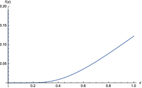
Figure 1: Plot of $\mathcal{P}=f(\epsilon)$ with $v=1$, $M=-2\pi$, $m=1$, $\omega=\sqrt{\epsilon}$.

Then the limit $\epsilon\rightarrow 0$ leads to $\mathcal{P}\approx 0$.

Proof.

of the proposition (2): The rest of this section is devoted to the proof of the proposition (2). The density $\Omega=:\Omega(\omega,\widetilde{\omega},E,B)$ such that $\mathcal{P}=\exp(-\Omega)$ can be expanded as

$$\Omega = \Omega_{1}(\omega,\widetilde{\omega},E,B)-\Omega_{2}(\omega,\widetilde{\omega},E,B),$$ (56)

where

$$\Omega_{1}=\int d{\bf x}\int_{0}^{\infty}\frac{ds}{s}\langle{\bf x}|e^{is\mathcal{Y}_{H}(\omega,\widetilde{\omega},E,B)}|{\bf x}\rangle,$$ (57)

$$\Omega_{2}=\int d{\bf x}\int_{0}^{\infty}\frac{ds}{s}\langle{\bf x}|e^{is\mathcal{X}_{H}(\omega,\widetilde{\omega})}|{\bf x}\rangle.$$ (58)

We consider the mean values:

$$x^{1}_{H} = <{\bf x}|\mathcal{X}^{1}_{H}|{\bf x}>,\quad x^{2}_{H}=<{\bf x}|\mathcal{X}^{2}_{H}|{\bf x}>,$$ (59)

$$y^{1}_{H} = <{\bf x}|\mathcal{Y}^{1}_{H}|{\bf x}>,\quad y^{2}_{H}=<{\bf x}|\mathcal{Y}^{2}_{H}|{\bf x}>.$$ (60)

Now we choose $\omega=v\widetilde{\omega}$ and $vt+x>0$ and we are focussing on the computation of $\Omega_{1}(\omega,\widetilde{\omega},E,B)$. We get

$$\Omega_{1} = \int_{0}^{\infty}\frac{ds}{s}\langle{\bf x}|e^{is\mathcal{Y}_{H}(0,0,E,B)}|{\bf x}\rangle$$ (61)

$$\times \int d{\bf x}d{\bf k}\,\Big{(}1+is\omega y^{1}_{H}+is\widetilde{\omega}y^{2}_{H}\Big{)}\qquad$$ (62)

with

$$\langle{\bf x}|e^{is\mathcal{Y}_{H}}|{\bf x}\rangle=\frac{-iEB\coth(Es)\cot(Bs)}{4\pi^{2}}e^{-ism^{2}}.$$ (63)

A simple routine checking shows that

$$\int d{\bf x}d{\bf k}\,\exp\Big{[}is\widetilde{\omega}\Big{(}vy^{1}_{H}+y^{2}_{H}\Big{)}\Big{]}$$ (64)

$$=\frac{M\pi^{2}e^{\pi}}{4s^{2}\epsilon}\int\,\frac{dxdt}{(vt+x)^{2}}\Big{\{}$$ (65)

$$\exp\Big{[}is\widetilde{\omega}\Big{(}-\frac{P(x,t)}{vt+x}+Q(x,t)\Big{)}\Big{]}\Big{\}}$$ (66)

with

$$P(x,t) = 2v^{2}(3+2Bxt\gamma^{0}\gamma^{2}+B^{2}x^{2}t^{2}$$ (67)

$$- 2\gamma^{0}\gamma^{3}Et^{2}+E^{2}t^{4})+2v(2Bx^{2}\gamma^{0}\gamma^{2}$$ (68)

$$+ i\gamma^{1}\gamma^{2}Bxt+2B^{2}x^{3}t-2\gamma^{0}\gamma^{3}Ext$$ (69)

$$- i\gamma^{1}\gamma^{3}Et^{2}+E^{2}xt^{3})+\frac{3}{2}+2i\gamma^{1}\gamma^{2}Bx^{2}$$ (70)

$$+ 2B^{2}x^{4}-2i\gamma^{1}\gamma^{3}Ext+2E^{2}x^{2}t^{2},$$ (71)

and

$$Q(x,t) = v\big{[}4\gamma^{0}\gamma^{2}Bx-6\gamma^{0}\gamma^{3}Et+2i\gamma^{1}\gamma^{2}Bt$$ (72)

$$+ 2t(B^{2}x^{2}+E^{2}t^{2})\big{]}-i\gamma^{1}\gamma^{3}Et$$ (73)

$$+ 3i\gamma^{1}\gamma^{2}Bx-2\gamma^{0}\gamma^{3}Ex$$ (74)

$$+ 2x(B^{2}x^{2}+E^{2}t^{2}).$$ (75)

In the same manner $\Omega_{2}$ takes the form

$$\Omega_{2} = \int_{0}^{\infty}\frac{ds}{s}\int d{\bf x}d{\bf k}\,\langle{\bf x}|e^{is\mathcal{X}_{H}(0,0)}|{\bf x}\rangle$$ (76)

$$\times \Big{(}1+is\omega x^{1}_{H}+is\widetilde{\omega}x^{2}_{H}\Big{)}$$ (77)

where

$$\langle{\bf x}|e^{is\mathcal{X}_{H}}|{\bf x}\rangle=-\frac{i}{16\pi^{2}s^{2}}e^{-ism^{2}}.$$ (78)

We can now show that

$$\int d{\bf x}d{\bf k}\,\Big{(}1+isv\widetilde{\omega}x^{1}_{H}+is\widetilde{\omega}x^{2}_{H}\Big{)}$$ (79)

$$=\int\,d{\bf x}\frac{\pi^{2}e^{\pi}}{4s^{2}\epsilon(vt+x)^{2}}\exp\Big{[}-\frac{3is\widetilde{\omega}(v^{2}+1)}{8(vt+x)}\Big{]}.$$ (80)

However

$$\Omega(\widetilde{\omega},E,B)=\frac{iMe^{\pi}}{64\epsilon}\int_{0}^{\infty}\,ds\,\frac{e^{-ism^{2}}}{s^{3}}\Big{[}\frac{1}{s^{2}}\mathcal{I}(t_{0},x_{0})$$ (82)

$$-4EB\coth(Es)\cot(Bs)\mathcal{J}(t_{0},x_{0})\Big{]}$$ (83)

where $M$ is chosen to be $M=\int\,\mu(x,y)dy\,dz<\infty,$

$$\mathcal{I}(t_{0},x_{0}) = \int_{x_{0}}^{\infty}\int_{t_{0}}^{\infty}\,dxdt\,\frac{\pi^{2}e^{\pi}}{4s^{2}\epsilon(vt+x)^{2}}\Big{\{}$$ (85)

$$\exp\Big{[}-\frac{3is\widetilde{\omega}(v^{2}+1)}{8(vt+x)}\Big{]}\Big{\}}$$

and

$$\mathcal{J}(t_{0},x_{0})=\int_{x_{0}}^{\infty}\int_{t_{0}}^{\infty}\,dxdt\,\frac{1}{(vt+x)^{2}}$$ (86)

$$\times\exp\Big{[}is\widetilde{\omega}\Big{(}-\frac{P(x,t)}{(vt+x)}+Q(x,t)\Big{)}\Big{]}.$$ (87)

The integral (82) exhibit the divergence at point $x=t=0$. This shall be regularized by using the Cauchy principal value. For $E=B=0$ we get

$$\mathcal{I}(0,0) = \frac{1}{\alpha_{1}}\int_{0}^{\infty}\,dt\,\Big{[}\sin(\alpha_{1}/vt)+2i\sin^{2}(\alpha_{1}/2vt)\Big{]}$$ (88)

$$= \frac{i\pi}{2v}+\frac{1}{v}\Big{[}1-N_{\gamma}-\ln\Big{(}\frac{\alpha_{1}}{v}\Big{)}\Big{]},$$ (89)

$$\mathcal{J}(0,0) = \frac{1}{\alpha_{2}}\int_{0}^{\infty}\,dt\,\Big{[}\sin(\alpha_{2}/vt)+2i\sin^{2}(\alpha_{2}/2vt)\Big{]}$$ (90)

$$= \frac{i\pi}{2v}+\frac{1}{v}\Big{[}1-N_{\gamma}-\ln\Big{(}\frac{\alpha_{2}}{v}\Big{)}\Big{]},$$ (91)

with $\alpha_{1}=\frac{3s\widetilde{\omega}}{8}(v^{2}+1)$, $\alpha_{2}=\frac{s\widetilde{\omega}}{2}(12v^{2}+3)$ and $N_{\gamma}$ is the Euler number given by $N_{\gamma}=0.577215664$. Also, for $a,b\in\mathbb{R}$ the integral

$$\mathcal{Q}=\int_{0}^{\infty}\,ds\,\frac{e^{-ism^{2}}}{s^{5}}\Big{(}4\ln(bs)-\ln(as)\Big{)}$$

admits the Cauchy principal value

$$Pv(\mathcal{Q}) = \frac{m^{8}}{1152}\Big{[}415-300N_{\gamma}+72N_{\gamma}^{2}+12\pi^{2}$$ (92)

$$+ 96\ln b^{2}-24\ln a^{2}-300\ln(im^{2})$$ (93)

$$+ 72\ln(im^{2})^{2}+144N_{\gamma}\ln(im^{2})$$ (94)

$$+ 4\Big{(}-25+12N_{\gamma}+12\ln(im^{2})\Big{)}\ln a$$ (95)

$$- 16\Big{(}-25+12N_{\gamma}+12\ln(im^{2})\Big{)}\ln b\Big{]}.$$ (96)

Remark that the probability density of pair creation in the limit $\widetilde{\omega}=0$ (see Lin:1998rn ) correspond to

$$\Omega(0,E,B)=\frac{EB}{4\pi^{2}}\sum_{k=1}^{\infty}\,\frac{1}{k}\coth\Big{(}k\pi\frac{B}{E}\Big{)}\exp\Big{(}-\frac{k\pi m^{2}}{E}\Big{)}.$$ (98)

Using the Taylor expansion as

$$\Omega(\widetilde{\omega},E,B)=\Omega(0,E,B)+\widetilde{\omega}\Omega^{\prime}(0,E,B)+\mathcal{O}(\widetilde{\omega}^{2}),$$ (99)

we come to $\Omega(\widetilde{\omega},0,0)=\widetilde{\omega}\Omega^{\prime}(0,0,0)+\mathcal{O}(\widetilde{\omega}^{2})$ and

$$\Omega(\widetilde{\omega},0,0)=\frac{iMe^{\pi}}{64\epsilon}\int_{0}^{\infty}\,ds\,\frac{e^{-ism^{2}}}{s^{5}}\mathcal{T}(0,0),$$ (100)

$$\mathcal{T}(0,0)=\mathcal{I}(0,0)-4\mathcal{J}(0,0).$$

We choose the real part of $\Omega(\widetilde{\omega},0,0)$ denoted by $\Re_{e}\Omega(\widetilde{\omega},0,0)=[\Omega(\widetilde{\omega},0,0)+\Omega^{*}(\widetilde{\omega},0,0)]/2$. Using (88), (90) and (92)

$$\Re_{e}\Omega(\widetilde{\omega},0,0) = -\frac{\pi Me^{\pi}m^{8}}{1024v\epsilon}\Big{[}2N_{\gamma}-\frac{37}{12}$$ (101)

$$- \frac{1}{3}\Big{(}4\ln b-\ln a\Big{)}\Big{]}.$$ (102)

where $a=\frac{3\widetilde{\omega}}{8v}(v^{2}+1)$, $b=\frac{3\widetilde{\omega}}{2v}(4v^{2}+1)$. Finally it is straightforward to check the following relation

$$\widetilde{\omega}\Omega^{\prime}(0,0,0) = \frac{\pi Me^{\pi}m^{8}}{1024v\epsilon}\Big{[}2N_{\gamma}-\frac{37}{12}$$ (103)

$$- \frac{1}{3}\Big{(}4\ln b-\ln a\Big{)}\Big{]}.$$ (104)

While the probability of the pair production takes the form

$$\mathcal{P} = \exp\Big{\{}-\frac{\pi Me^{\pi}m^{8}}{1024v\epsilon}\Big{[}2N_{\gamma}-\frac{37}{12}$$ (105)

$$- \frac{1}{3}\Big{(}4\ln b-\ln a\Big{)}\Big{]}\Big{\}}\approx 0.$$ (106)

This end the proof of proposition (2). ∎

IV Solution of the Dirac equation

In this section we give the solution of the Dirac equation (26). We consider the operators $\mathcal{K}_{1}$ and $\mathcal{K}_{2}$ satisfying the commutation relation $[\mathcal{K}_{1},\mathcal{K}_{2}]=0$ and given by

$$\mathcal{K}_{1} = i\gamma^{0}\partial_{0}-i\gamma^{2}k_{2}-i\gamma^{3}k_{3}+i\gamma^{3}Et+9i\omega\gamma^{0}$$ (108)

$$-3\widetilde{\omega}\gamma^{1}-m(1-\omega t),$$

$$\mathcal{K}_{2}=-\gamma^{1}\partial_{1}-i\gamma^{2}Bx+m\widetilde{\omega}x.$$ (109)

The equation (26) takes the form $(\mathcal{K}_{1}+\mathcal{K}_{2})\psi(t,x)=0$ and admit separate variables as $\psi(t,x)=\psi(t)\psi(x)$. For a constant $\lambda\in\mathbb{C}$, we get the two eigenvalue equations

$$\mathcal{K}_{1}\psi(t,x)=\lambda\psi(t,x)$$ (110)

$$\mathcal{K}_{2}\psi(t,x)=\lambda\psi(t,x).$$ (111)

Consider the equation (110). We write the four vector $\psi(t)$ as $\psi(t)=(\psi_{1}(t),\psi_{2}(t))$ and $\psi_{j}(t)=(\psi_{ja}(t),\psi_{jb}(t)),\,\,j=1,2$, and the equation (110) leads to

$$\big{(}{L^{\prime}L}+{D^{2}}+CC^{\prime}\big{)}\psi_{1a}(t)=0,$$ (112)

$$\big{(}{LL^{\prime}}+{D^{2}}+CC^{\prime}\big{)}\psi_{2a}(t)=0,$$ (113)

$$C\psi_{1b}(t)={L^{\prime}}\psi_{2a}(t)-{D}\psi_{1a}(t),$$ (114)

$$C\psi_{2b}(t)=-{L}\psi_{1a}(t)-{D}\psi_{2a}(t)$$ (115)

where

$$L=i\partial_{0}+9i\omega-m(1-\omega t)+\lambda,$$

$$L^{\prime}=-i\partial_{0}-9i\omega+m(1-\omega t)+\lambda$$

$$C=-3\widetilde{\omega}-k_{2},\quad C^{\prime}=-3\widetilde{\omega}+k_{2},$$

$$D=iEt-ik_{3}.$$

Let

$$f(t) = \frac{E}{2}t^{2}+\Big{(}\frac{m}{E}(m-\lambda)\omega-9\omega-k_{3}\Big{)}t,$$ (116)

$$g(t) = (-1)^{1\over 4}(iE)^{\frac{1}{2}}t$$ (117)

$$\delta^{1}_{E} = \frac{m\omega}{2E^{3}}(m-\lambda)$$ (118)

$$+ \frac{1}{2E}\Big{(}k_{2}^{2}-(m-\lambda)^{2}+im\omega\Big{)}-\frac{1}{2}$$ (119)

$$\delta^{2}_{E} = \frac{(-1)^{1\over 4}}{(iE)^{\frac{3}{2}}}\Big{(}Ek_{3}-(m-\lambda)m\omega\Big{)}.$$ (120)

The solution of the equations (112) are a linear combination of Hermite and (1,1)-hypergeometric polynomial given by

$$\psi_{1a}(t) = c_{1}e^{f(t)}\mathcal{H}\Big{[}\delta^{1}_{E},\delta^{2}_{E}+g(t)\Big{]}$$ (121)

$$+ c_{2}e^{f(t)}{}_{1}F_{1}[\frac{\delta^{1}_{E}}{2},\frac{1}{2},\big{(}\delta^{2}_{E}+g(t)\big{)}^{2}]$$ (122)

$$\psi_{2a}(t) = c_{1}e^{f(t)}\mathcal{H}\Big{[}\bar{\delta}^{1}_{E},\delta^{2}_{E}+g(t)\Big{]}$$ (123)

$$+ c_{2}e^{f(t)}{}_{1}F_{1}[\frac{\bar{\delta}^{1}_{E}}{2},\frac{1}{2},\big{(}\delta^{2}_{E}+g(t)\big{)}^{2}].$$ (124)

the solutions of the equation (114) can be simple obtained using the followings identities:

$$\frac{d\,\mathcal{H}(a,b+ct)}{dt}=2ac\mathcal{H}(-1+a,b+ct),$$ (125)

$$\frac{d\,{}_{1}F_{1}(a,b,ct^{2}+dt+e)}{dt}$$ (126)

$$=\frac{a(d+2ct)}{b}{}_{1}F_{1}(1+a,1+b,ct^{2}+dt+e).$$ (127)

Now, consider the equation (111). Using the Dirac matrices (10), we get

$$-(\sigma_{1}\partial_{1}+i\sigma_{2}Bx)\psi_{2}(x)+(m\widetilde{\omega}x-\lambda)\psi_{1}(x)=0$$ (128)

$$(\sigma_{1}\partial_{1}+i\sigma_{2}Bx)\psi_{1}(x)+(m\widetilde{\omega}x-\lambda)\psi_{2}(x)=0$$ (129)

where $\psi(x)=(\psi_{1}(x),\psi_{2}(x))$. Let us define the quantities $b(B)$, $r(B)$ and $s(B)$ as

$$b(B)=:\frac{\lambda^{2}}{2B},$$

$$r(B)=\frac{2m\widetilde{\omega}\lambda(-1)^{\frac{1}{4}}}{\sqrt{2}(iB)^{\frac{3}{2}}},$$

$$s(B)=(-1)^{\frac{1}{4}}\sqrt{2}(iB)^{\frac{1}{2}}.$$

For $\psi_{j}(x)=(\psi_{ja}(x),\psi_{jb}(x)),\,\,j=1,2$. The solutions of the equation (128) are

$$\psi_{1a}(x) = c_{1}\mathcal{D}\Big{[}-b(B),-r(B)+s(B)x\Big{]}$$ (130)

$$+ c_{2}\mathcal{\mathcal{missing}}D\Big{[}-b(B),-ir(B)+is(B)x\Big{]}$$ (131)

$$\psi_{1b}(x) = c_{1}\mathcal{D}\Big{[}-1-b(B),-r(B)+s(B)x\Big{]}$$ (132)

$$+ c_{2}\mathcal{D}\Big{[}-1-b(B),-ir(B)+is(B)x\Big{]}.$$ (133)

However, the equation (129) can be split into

$$\Big{[}\partial_{1}^{2}-B-B^{2}x^{2}+\lambda^{2}-2m\lambda\widetilde{\omega}x\Big{]}\psi_{1a}(x)=0$$ (135)

$$\Big{[}\partial_{1}^{2}+B-B^{2}x^{2}+\lambda^{2}-2m\lambda\widetilde{\omega}x\Big{]}\psi_{1b}(x)=0,$$ (136)

and the solutions are well given by the following:

$$\psi_{2a}(x)=\frac{1}{\lambda-m\widetilde{\omega}x}(\partial_{1}+Bx)\psi_{1b},$$ (137)

$$\psi_{2b}(x)=\frac{1}{\lambda-m\widetilde{\omega}x}(\partial_{1}-Bx)\psi_{1a}.$$ (138)

where the identities

$$\frac{d}{dx}\mathcal{D}(a,bx+c) = \frac{b}{2}(bx+c)\mathcal{D}(a,bx+c)$$ (139)

$$- b\mathcal{D}(1+a,bx+c),$$ (140)

are usefull.

V Conclusion

In this paper, we have computed the probability density of pair production of the fermion particles. The case of vanishing EM fields is scrutinized explicitly. Hereafter we will shed light on the case of non-vanishing EM fields, which has not been entirely considered in this paper. In the other hand, we have solved the Dirac equation coupled with gravitation field, using the separation of variables. The solutions are expressed in terms of hypergeometric functions. The limit where the deformation parameter $\widetilde{\omega}$ tends to zero is given.

References

- (1) S. P. Gavrilov and D. M. Gitman, “Vacuum instability in external fields,” Phys. Rev. D 53, 7162 (1996) [hep-th/9603152].
- (2) Q. -G. Lin, “Electron - positron pair creation in vacuum by an electromagnetic field in (3+1)-dimensions and lower dimensions,” J. Phys. G 25, 17 (1999) [hep-th/9810037].
- (3) N. Chair and M. M. Sheikh-Jabbari, “Pair production by a constant external field in noncommutative QED,” Phys. Lett. B 504, 141 (2001) [hep-th/0009037].
- (4) E. Brezin and C. Itzykson, “Pair production in vacuum by an alternating field,” Phys. Rev. D 2, 1191 (1970).
- (5) T. C. Adorno, S. P. Gavrilov and D. M. Gitman, “Particle creation from the vacuum by an exponentially decreasing electric field,” arXiv:1409.7742 [hep-th].
- (6) D. Ousmane Samary, E. E. N’Dolo and M. N. Hounkonnou, “Pair production of Dirac particles in a -dimensional noncommutative space–time,” Eur. Phys. J. C 74, no. 11, 3165 (2014) [arXiv:1406.0219 [hep-th]].
- (7) G. V. Shishkin and V. M. Villalba, “Neutrino in the presence of gravitational fields: Exact solutions,” J. Math. Phys. 33, 4037 (1992).
- (8) V. M. Villalba, “Exact solution of the Dirac equation in the presence of a gravitational instanton,” J. Phys. Conf. Ser. 24, 136 (2005).
- (9) V. M. Villalba and W. Greiner, “Creation of Dirac particles in the presence of a constant electric field in an anisotropic Bianchi I universe,” Mod. Phys. Lett. A 17, 1883 (2002) [gr-qc/0211005].
- (10) V. M. Villalba, “Creation of scalar particles in the presence of a constant electric field in an anisotropic cosmological universe,” Phys. Rev. D 60, 127501 (1999) [hep-th/9909074].
- (11) G. V. Shishkin and V. M. Villalba, “Neutrino in the presence of gravitational fields: Separation of variables,” J. Math. Phys. 33, 2093 (1992).
- (12) Y. Sucu and N. Unal, “Exact solution of Dirac equation in 2+1 dimensional gravity,” J. Math. Phys. 48, 052503 (2007).
- (13) V. M. Villalba, “Exact Solution To The Dirac Equation In The Presence Of An Exact Gravitational Plane Wave,” Phys. Lett. A 136, 197 (1989).
- (14) V. M. Villalba, “Separation of variables and exact solution to the Dirac equation in nonstatic Minkowski space-times,” J. Phys. A 24, 3781 (1991).
- (15) M. N. Hounkonnou and J. E. B. Mendy, “Exact solutions of Dirac equation for neutrinos in presence of external fields,” J. Math. Phys. 40, 4240 (1999).
- (16) M. Arminjon, “Some Remarks on Quantum Mechanics in a Curved Spacetime, Especially for a Dirac Particle,” Int. J. Theor. Phys. 54, no. 7, 2218 (2015).
- (17) M. Cariglia, “Hidden Symmetries of the Dirac Equation in Curved Space-Time,” Springer Proc. Phys. 157, 25 (2014) [arXiv:1209.6406 [gr-qc]].
- (18) J. Yepez, “Einstein’s vierbein field theory of curved space,” arXiv:1106.2037 [gr-qc].
- (19) R. Muehlhoff, “Higher Spin Quantum Fields as Twisted Dirac Fields,” arXiv:1103.4826 [math-ph].
- (20) M. D. Pollock, “On the Dirac equation in curved space-time,” Acta Phys. Polon. B 41, 1827 (2010).
- (21) V. F. Muller, “Dirac Quantum Field on Curved Spacetime: Wick Rotation,” arXiv:1002.3263 [hep-th].
- (22) M. Arminjon and F. Reifler, “A Non-uniqueness problem of the Dirac theory in a curved spacetime,” Annalen Phys. 523, 531 (2011) [arXiv:0905.3686 [gr-qc]].
- (23) F. Cianfrani and G. Montani, “Curvature-spin coupling from the semi-classical limit of the Dirac equation,” Int. J. Mod. Phys. A 23, 1274 (2008) [arXiv:0805.2480 [gr-qc]].
- (24) J. B. Griffiths, “On Dirac Fields In A Curved Space-time,” J. Phys. A 12, 2429 (1979).
- (25) T. P. Hack, “Cosmological Applications of Algebraic Quantum Field Theory in Curved Spacetimes,” arXiv:1506.01869 [gr-qc].
- (26) K. Fredenhagen and T. P. Hack, “Quantum field theory on curved spacetime and the standard cosmological model,” Lect. Notes Phys. 899, 113 (2015) [arXiv:1308.6773 [math-ph]].
- (27) M. Benini, C. Dappiaggi and T. P. Hack, “Quantum Field Theory on Curved Backgrounds – A Primer,” Int. J. Mod. Phys. A 28, 1330023 (2013) [arXiv:1306.0527 [gr-qc]].