Measuring subhalo mass in redMaPPer clusters with CFHT Stripe 82 Survey

Abstract

We use the shear catalog from the CFHT Stripe-82 Survey to measure the subhalo masses of satellite galaxies in redMaPPer clusters. Assuming a Chabrier Initial Mass Function (IMF) and a truncated NFW model for the subhalo mass distribution, we find that the sub-halo mass to galaxy stellar mass ratio increases as a function of projected halo-centric radius $r_{p}$, from $M_{\rm sub}/M_{\rm star}=4.43^{+6.63}_{-2.23}$ at $r_{p}\in[0.1,0.3]$ ${\rm h^{-1}Mpc}$ to $M_{\rm sub}/M_{\rm star}=75.40^{+19.73}_{-19.09}$ at $r_{p}\in[0.6,0.9]$ ${\rm h^{-1}Mpc}$. We also investigate the dependence of subhalo masses on stellar mass by splitting satellite galaxies into two stellar mass bins: $10<\log(M_{\rm star}/\rm{h^{-1}M_{\odot}})<10.5$ and $11<\log(M_{\rm star}/\rm{h^{-1}M_{\odot}})<12$. The best-fit subhalo mass of the more massive satellite galaxy bin is larger than that of the less massive satellites: $\log(M_{\rm sub}/\rm{h^{-1}M_{\odot}})=11.14^{+0.66}_{-0.73}$ ($M_{\rm sub}/M_{\rm star}=19.5^{+19.8}_{-17.9}$) versus $\log(M_{\rm sub}/\rm{h^{-1}M_{\odot}})=12.38^{+0.16}_{-0.16}$ ($M_{\rm sub}/M_{\rm star}=21.1^{+7.4}_{-7.7}$).

1 Introduction

In a cold dark matter (CDM) universe, dark matter haloes form hierarchically through accretion and merging(for a recent review, see Frenk & White (2012)). Many rigorous and reliable predictions for the halo mass function and subhalo mass functions in CDM are provided by numerical simulations(e.g. Springel et al., 2008; Gao et al., 2011; Colín et al., 2000; Hellwing et al., 2015; Bose et al., 2016). When the small haloes merge to the larger systems, they become the subhaloes and suffer from environmental effects such as tidal stripping, tidal heating and dynamical friction that tend to remove the mass from them and even disrupt them (Tormen et al., 1998; Taffoni et al., 2003; Diemand et al., 2007; Hayashi et al., 2003; Gao et al., 2004; Springel et al., 2008; Xie & Gao, 2015) . At the mean time, the satellite galaxies that reside in the subhaloes also experience environmental effects. The tidal stripping and ram-pressure can remove the hot gas halo from satellite galaxies which in turn cuts off their supply of cold gas and quenches star formation(Balogh et al., 2000; Kawata & Mulchaey, 2008; McCarthy et al., 2008; Wang et al., 2007; Guo et al., 2011; Wetzel et al., 2013). Satellite galaxies in some cases also experience a mass loss in the cold gas component and stellar component during the interaction with the host haloes (Gunn & Gott, 1972; Abadi et al., 1999; Chung et al., 2009; Mayer et al., 2001; Klimentowski et al., 2007; Kang & van den Bosch, 2008; Chang et al., 2013).

Overall, the subhaloes preferentially lose their dark mass rather than the luminous mass, because the mass distribution of satellite galaxies is much more concentrated than that of the dissipationless dark matter particles. Simulations predict that the mass loss of infalling subhaloes depends inversely on their halo-centric radius (e.g. Springel et al., 2001; De Lucia et al., 2004; Gao et al., 2004; Xie & Gao, 2015). Thus, the halo mass to stellar mass ratio of satellite galaxies should increase as a function of halo-centric radius. Mapping the mass function of subhaloes from observations can provide important constraints on this galaxy evolution model.

In observations, dark matter distributions are best measured with gravitational lensing. For dark matter subhalos, however, such observations are challenging due to their relative low mass compared to that of the host dark matter halo. The presence of subhalos can cause flux-ratio anomalies in multiply imaged lensing systems (Mao & Schneider, 1998; Metcalf & Madau, 2001; Mao et al., 2004; Xu et al., 2009; Nierenberg et al., 2014), perturb the locations, and change the image numbers (Kneib et al., 1996; Kneib & Natarajan, 2011), and disturb the surface brightness of extended Einstein ring/arcs (Koopmans, 2005; Vegetti & Koopmans, 2009a, b; Vegetti et al., 2010, 2012). However, due to the limited number of high quality images and the rareness of strong lensing systems, only a few subhalos have been detected through strong lensing observation. Besides, strong lensing effects can only probe the central regions of dark matter haloes (Kneib & Natarajan, 2011). Therefore, through strong lensing alone, it is difficult to draw a comprehensive picture of the co-evolution between subhalos and galaxies.

Subhalos can also be detected in individual clusters through weak gravitational lensing or weak lensing combining strong lensing (e.g. Natarajan et al., 2007; Natarajan et al., 2009; Limousin et al., 2005, 2007; Okabe et al., 2014). In Natarajan et al. (2009), Hubble Space Telescope images were used to investigate the subhalo masses of $L^{*}$ galaxies in the massive, lensing cluster, Cl0024+16 at z = 0.39, and to study the subhalo mass as a function of halo-centric radius. Okabe et al. (2014) investigated subhalos in the very nearby Coma cluster with imaging from the Subaru telescope. The deep imaging and the large apparent size of the cluster allowed them to measure the masses of subhalos selected by shear alone. They found 32 subhalos in the Coma cluster and measured their mass function. However, this kind of study requires very high quality images of massive nearby clusters, making it hard to extend such studies to large numbers of clusters.

A promising alternative way to investigate the satellite-subhalo relation is through a stacking analysis of galaxy-galaxy lensing with large surveys. Different methods have been proposed in previous studies (e.g. Yang et al., 2006; Li et al., 2013; Pastor Mira et al., 2011; Shirasaki, 2015). Although the tangential shear generated by a single subhalo is small, by stacking thousands of satellite galaxies the statistical noise can be suppressed and the mean projected density profile around satellite galaxies can be measured. Li et al. (2014) selected satellite galaxies in the SDSS group catalog from (Yang et al., 2007) and measured the weak lensing signal around these satellites with a lensing source catalog derived from the CFHT Stripe82 Survey (Comparat et al., 2013). This was the first galaxy-galaxy lensing measurement of subhalo masses in galaxy groups. However, the uncertainties of the measured subhalo masses were too large to investigate the satellite-subhalo relation as a function of halo-centric radius.

In this paper, we apply the same method as Li et al. (2013); Li et al. (2014) to measure the galaxy-galaxy lensing signal for satellite galaxies in the SDSS redMaPPer cluster catalog (Rykoff et al., 2014; Rozo & Rykoff, 2014). Unlike the the group catalog of Yang et al. (2007) which is constructed using SDSS spectroscopic galaxies, the redMaPPer catalog relies on photometric cluster detections, allowing it to go to higher redshifts. As a result, there are more massive clusters in the redMaPPer cluster catalog. Therefore, we expect to signal-to-noise of the satellite galaxy lensing signals to be higher, enabling us to derive better constraints on subhalo properties.

The paper is organized as follows. In section 2, we describe the lens and source catalogs. In section 3, we present our lens model. In section 4, we show our observational results and our best fit lens model. The discussions and conclusions are presented in section 5. Throughout the paper, we adopt a $\Lambda$CDM cosmology with parameters given by the WMAP-7-year data (Komatsu et al., 2010) with $\Omega_{L}=0.728$, $\Omega_{M}=0.272$ and $h\equiv H_{0}/(100{\rm kms^{-1}Mpc^{-1}})=0.73$. In this paper, stellar mass is estimated assuming a Chabrier (2003) IMF.

2 Observational Data

2.1 Lens selection and stellar masses

We use satellite galaxies in the redMaPPer clusters as lenses. The redMaPPer cluster catalog is extracted from photometric galaxy samples of the SDSS Data Release 8 (DR8, Aihara et al., 2011) using the red-sequence Matched-filter Probabilistic Percolation cluster finding algorithm (Rykoff et al., 2014). The redMaPPer algorithm uses the 5-band $(ugriz)$ magnitudes of galaxies with a magnitude cut $i<21.0$ over a total area of 10,000 deg² to photometrically detect galaxy clusters.

redMaPPer uses a multi-color richness estimator $\lambda$, defined to be the sum of the membership probabilities over all galaxies. In this work, we use clusters with richness $\lambda>20$ and photometric redshift $z_{\rm cluster}<0.5$. In the overlapping region with the CFHT Stripe-82 Survey, we have a total of 634 clusters. For each redMaPPer cluster, member galaxies are identified according to their photometric redshift, color and their cluster-centric distance. To reduce the contamination induced by fake member galaxies, we only use satellite galaxies with membership probability $P_{\rm mem}>0.8$. The redMaPPer cluster finder identifies 5 central galaxy candidates for each cluster, each with an estimate of the probability $P_{\rm cen}$ that the galaxy in question is the central galaxy of the cluster. We remove all central galaxy candidates from our lens sample. For more details about redMaPPer cluster catalog, we refer the readers to Rykoff et al. (2014); Rozo & Rykoff (2014).

Stellar masses are estimated for member galaxies in the redMaPPer catalog using the Bayesian spectral energy distribution (SED) modeling code iSEDfit (Moustakas et al., 2013). Briefly, iSEDfit determines the posterior probability distribution of the stellar mass of each object by marginalizing over the star formation history, stellar metallicity, dust content, and other physical parameters which influence the observed optical/near-infrared SED. The input data for each galaxy includes: the SDSS $ugriz$ model fluxes scaled to the $r$-band cmodel flux; the 3.4- and 4.6-$\micron$ “forced” WISE (Wright et al., 2010) photometry from Lang et al. (2014); and the spectroscopic or photometric redshift for each object inferred from redMaPPer. We adopt delayed, exponentially declining star formation histories with random bursts of star formation superposed, the Flexible Stellar Population Synthesis (FSPS) model predictions of Conroy et al. (2009, 2010), and the Chabrier (2003) initial mass function (IMF) from 0.1-100 $M_{\odot}$. For reference, adopting the Salpeter (1955) IMF would yield stellar masses which are on average 0.25 dex (a factor of 1.8) larger. We apply a stellar mass cut of $M_{\rm star}>10^{10}\rm{h^{-1}M_{\odot}}$ to our satellite galaxy sample. In Fig.1, we show the $M_{\rm star}$–$z_{l}$ distribution for our lens samples, where $z_{l}$ is the photometric redshift of the satellite galaxy assigned by the redMaPPer algorithm. The low stellar mass satellite galaxies are incomplete at higher redshift, but they will not affect the conclusion of this paper.

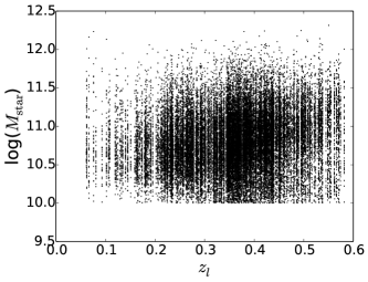
Figure 1: The $M_{\rm star}$–$z_{l}$ distribution of lens galaxies, where $z_{l}$ is the photometric redshift, and $M_{\rm star}$ is in units of $M_{\odot}$.

2.2 The Source Catalog

The source catalog is measured from the Canada–France–Hawaii Telescope Stripe 82 Survey (CS82), which is an $i-$band imaging survey covering the SDSS Stripe82 region. With excellent seeing conditions — FWHM between 0.4 to 0.8 arcsec — the CS82 survey reaches a depth of $i_{\rm AB}\sim 24.0$. The survey contains a total of 173 tiles, 165 of which from CS82 observations and 8 from CFHT-LS Wide (Erben et al., 2013). The CS82 fields were observed in four dithered observations with 410s exposure. The 5$\sigma$ limiting magnitude is $i_{\rm AB}\sim 24.0$ in a 2 arcsec diameter aperture.

Each CFHTLenS science image is supplemented by a mask, indicating regions within which accurate photometry/shape measurements of faint sources cannot be performed, e.g. due to extended haloes from bright stars. According to Erben et al. (2013), most of the science analysis are safe with sources with MASK$\leq 1$. After applying all the necessary masks and removing overlapping regions, the effective survey area reduces from 173 deg² to 129.2 deg². We also require that source galaxies to have FITCLASS= 0, where FITCLASS is the flag that describes the star/galaxy classification.

Source galaxy shapes are measured with the lensfit method (Miller et al., 2007; Miller et al., 2013), closely following the procedure in Erben et al. (2009, 2013). The shear calibration and systematics of the lensfit pipeline are described in detail in Heymans et al. (2012). The specific procedures that are applied to the CS82 imaging are described in Erben et al. (2015, in preparation).

Since the CS82 survey only provides the $i$-band images, the CS82 collaboration derived source photometric redshifts using the $ugriz$ multi-color data from the SDSS co-add (Annis et al., 2014), which reaches roughly 2 magnitudes deeper than the single epoch SDSS imaging. The photometric redshift (photo-z) of the background galaxies were estimated using a Bayesian photo-$z$ code (BPZ, Benítez, 2000; Bundy et al., 2015). The effective weighted source galaxy number density is 4.5 per arcmin². Detailed systematic tests for this weak lensing catalog are described in Leauthaud et al. 2015 (in prep).

2.3 Lensing Signal Computation

In a galaxy-galaxy lensing analysis, the excess surface mass density , $\Delta\Sigma$ is inferred by measuring the tangential shear, $\gamma_{t}(R)$, where

$$\Delta\Sigma(R)=\gamma_{t}(R)\Sigma_{\rm crit}={\overline{\Sigma}}(<R)-\Sigma(R)\,,$$ (1)

where ${\overline{\Sigma}}(<R)$ is the mean surface mass density within $R$, and $\Sigma(R)$ is the average surface density at the projected radius $R$, and $\Sigma_{\rm crit}$ is the lensing critical surface density

$$\Sigma_{\rm crit}=\frac{c^{2}}{4\pi G}\frac{D_{s}}{D_{l}D_{ls}}\,,$$ (2)

where $D_{ls}$ is the angular diameter distance between the lens and the source, and $D_{l}$ and $D_{s}$ are the angular diameter distances from the observer to the lens and to the source, respectively.

We select satellite galaxies as lenses and stack lens-source pairs in physical radial distance $R$ bins from $0.04$ to $1.5{\rm h^{-1}Mpc}$. To avoid contamination from foreground galaxies, we remove lens-source pairs with $z_{s}-z_{l}<0.1$, where $z_{s}$ and $z_{l}$ are lens redshift and source redshift respectively. We have also tested the robustness of our results by varying the selection criteria for source galaxies. We find that selecting lens-source pairs with $z_{s}-z_{l}>0.05$ or $z_{s}-z_{l}>0.15$ only changes the final lensing signal by less than 7%, well below our final errors.

For a given set of lenses, $\Delta\Sigma(R)$ is estimated using

$$\Delta\Sigma(R)=\frac{\sum_{l}\sum_{s}w_{ls}\gamma_{t}^{ls}\Sigma_{\rm crit}(z_{l},z_{s})}{\sum_{l}\sum_{s}w_{ls}}\,,$$ (3)

where

$$w_{ls}=w_{n}\Sigma_{\rm crit}^{-2}(z_{l},z_{s})\,$$ (4)

and $w_{n}$ is a weight factor defined by Eq.  (8) in Miller et al. (2013). $w_{n}$ is introduced to account for the intrinsic distribution of ellipticity and shape measurement uncertainties.

In the lensfit pipeline, a calibration factor for the multiplicative error $m$ is estimated for each galaxy based on its signal-to-noise ratio, and the size of the galaxy. Following Miller et al. (2013), we account for these multiplicative errors in the stacked lensing by the correction factor

$$1+K(R)=\frac{\sum_{l}\sum_{s}w_{ls}(1+m_{s})}{\sum_{l}\sum_{s}w_{ls}}$$ (5)

The corrected lensing measurement is as:

$$\Delta\Sigma(R)^{\rm corrected}=\frac{\Delta\Sigma(R)}{1+K(R)}$$ (6)

In this paper, we stack the tangential shears around satellite galaxies binned according to their projected halo-centric distance $r_{p}$, and fit the galaxy-galaxy lensing signal to obtain the subhalo mass of the satellite galaxies. We describe our theoretical lens models below.

3 The Lens Model

The surface density around a lens galaxy $\Sigma(R)$ can be written as:

$$\Sigma(R)=\int_{0}^{\infty}\rho_{\rm g,m}\left(\sqrt{R^{2}+\chi^{2}}\right)\,{\rm d}\chi\,;$$ (7)

and the mean surface density within radius $R$ is

$$\Sigma(<R)=\frac{2}{R^{2}}\int_{0}^{R}\Sigma(u)\,u\,{\rm d}u,$$ (8)

where $\rho_{g,m}$ is the density profile around the lens, and $\chi$ is the physical distance along the line of sight. The excess surface density around a satellite galaxy is composed of three components:

$$\Delta\Sigma(R)=\Delta\Sigma_{\rm sub}(R)+\Delta\Sigma_{\rm host}(R,r_{p})+\Delta\Sigma_{\rm star}(R)\,,$$ (9)

where $\Delta\Sigma_{\rm sub}(R)$ is the contribution of the subhalo in which the satellite galaxy resides, $\Delta\Sigma_{\rm host}(R,r_{p})$ is the contribution from the host halo of the cluster/group, where $r_{p}$ is the projected distance from the satellite galaxy to the center of the host halo, and $\Delta\Sigma_{\rm star}(R)$ is the contribution from the stellar component of the satellite galaxy. We neglect the two-halo term, which is the contribution from other haloes on the line-of-sight, because this contribution is only important at $R>3{\rm h^{-1}Mpc}$ for clusters (see Shan et al., 2015). At small scales where the subhalo term dominates, the contribution of the 2-halo term is at least an order of magnitude smaller than the subhalo term (Li et al., 2009).

3.1 Host halo contribution

We assume that host haloes are centered on the central galaxies of clusters, with a density profile following the NFW (Navarro et al., 1997) formula:

$$\rho_{\rm host}(r)=\frac{\rho_{\rm 0,host}}{(1+r/r_{\rm s,host})^{2}(r/r_{\rm s,host})}\,,$$ (10)

where $r_{\rm s,host}$ is the characteristic scale of the halo and $\rho_{\rm 0,host}$ is a normalization factor. Given the mass of a dark matter halo, its profile then only depends on the concentration parameter $c\equiv r_{\rm 200}/r_{\rm s,host}$, where $r_{\rm 200}$ is a radius within which the average density of the halo equals to 200 times the universe critical density, $\rho_{\rm crit}$. The halo mass $M_{\rm 200}$ is defined as $M_{\rm 200}\equiv 4\pi/3r_{\rm 200}^{3}(200\rho_{\rm crit})$.

Various fitting formulae for mass-concentration relations have been derived from N-body numerical simulations (e.g. Bullock et al., 2001; Zhao et al., 2003; Dolag et al., 2004; Macciò et al., 2007; Zhao et al., 2009; Duffy et al., 2008; Neto et al., 2007). These studies find that the concentration decreases with increasing halo mass. Weak lensing observations also measure this trend, but the measured amplitude of the mass-concentration relation is slightly smaller than that in the simulation (e.g. Mandelbaum et al., 2008; Miyatake et al., 2013; Shan et al., 2015). Since there is almost no degeneracy between the subhalo mass and the concentration (Li et al., 2013; George et al., 2012), we expect that the exact choice of the mass-concentration relation should not have a large impact on our conclusions. Throughout this paper, we adopt the mass concentration relation from Neto et al. (2007):

$$c=4.67(M_{\rm 200}/10^{14}\rm{h^{-1}M_{\odot}})^{-0.11}$$ (11)

We stack satellite galaxies with different halo-centric distance $r_{p}$, and in host halos with different mass. Thus the lensing contribution from the host halo is an average of $\Delta{\Sigma}_{\rm host}$ over $r_{p}$ and host halo mass $M_{\rm 200}$. The host halo profile is modeled as follows.

For each cluster, we can estimate its mass via the richness-mass relation of Rykoff et al. (2012):

$$\ln{\left(\frac{M_{\rm 200}}{h_{\rm 70}^{-1}10^{14}M_{\odot}}\right)}=1.48+1.06\ln(\lambda/60)$$ (12)

In the redMaPPer catalog, each cluster has five possible central galaxies, each with probability $P_{\rm cen}$. We assume that the average $\Delta\Sigma$ contribution from the host halo to a satellite can be written as:

$$\Delta\bar{\Sigma}_{\rm host}(R)=A_{0}\sum_{i}^{N_{\rm sat}}\sum_{j}^{5}\Delta\Sigma_{\rm host}(R|r_{\rm p,j},M_{\rm 200})P_{\rm cen,j}\,,$$ (13)

where $r_{\rm p,j}$ is the projected distance between the satellite and the jth candidate of the host cluster center, $P_{\rm cen,j}$ is the probability of jth candidate to be the true center, and $N_{\rm sat}$ is the number of stacked satellite galaxies. $A_{0}$ is the only free parameter of the host halo contribution model. It describes an adjustment of the lensing amplitude. If the richness-mass relation is perfect, the best-fit $A_{0}$ should be close to unity. Note that, the subhalo mass determination is robust against the variation of the normalization in richness-mass relation. If we decrease the normalization in Eq. 12 by 20%, the best-fit subhalo mass changes only by 0.01 dex, which is at least 15 times smaller than the $1\sigma$ uncertainties of $M_{\rm sub}$ (see table 2).

3.2 Satellite contribution

In numerical simulations, subhalo density profiles are found to be truncated in the outskirts (e.g. Hayashi et al., 2003; Springel et al., 2008; Gao et al., 2004; Xie & Gao, 2015). In this work, we use a truncated NFW profile (Baltz et al., 2009; Oguri & Hamana, 2011, tNFW, hereafter) to describe the subhalo mass distribution:

$$\rho_{\rm sub}(r)=\frac{\rho_{0}}{r/r_{s}(1+r/r_{s})^{2}}\left(\frac{r_{t}^{2}}{r^{2}+r_{t}^{2}}\right)^{2}\,$$ (14)

where $r_{t}$ is the truncation radius of the subhalo, $r_{s}$ is the characteristic radius of the tNFW profile and $\rho_{0}$ is the normalization. The enclosed mass with $x\equiv r/r_{s}$ can be written as:

$$M(<x) = 4\pi\rho_{0}r_{s}^{3}\frac{\tau^{2}}{2(\tau^{2}+1)^{3}(1+x)(\tau^{2}+x^{2})}$$ (15)

$$\times\Bigl{[}(\tau^{2}+1)x\left\{x(x+1)-\tau^{2}(x-1)(2+3x)-2\tau^{4}\right\}$$

$$+\tau(x+1)(\tau^{2}+x^{2})\left\{2(3\tau^{2}-1){\rm arctan}(x/\tau)\right.$$

$$\left.+\tau(\tau^{2}-3)\ln(\tau^{2}(1+x)^{2}/(\tau^{2}+x^{2}))\right\}\Bigr{]},$$

where $\tau\equiv r_{t}/r_{s}$. We define the subhalo mass $M_{\rm sub}$ to be the total mass within $r_{t}$. Given $M_{\rm sub}$, $r_{s}$ and $r_{t}$, the tangential shear $\gamma_{t}$ can be derived analytically (see the appendix in Oguri & Hamana (2011)).

Previous studies have sometimes used instead the pseudo-isothermal elliptical mass distribution (PIEMD) model derived by Kassiola & Kovner (1993)) for modeling the mass distribution around galaxies (e.g. Limousin et al., 2009; Natarajan et al., 2009; Kneib & Natarajan, 2011). The surface density of the PIEMD model can be written as:

$$\Sigma(R)=\frac{\Sigma_{0}R_{0}}{1-R_{0}/R_{t}}\left(\frac{1}{\sqrt{R_{0}^{2}+R^{2}}}-\frac{1}{\sqrt{R_{t}^{2}+R^{2}}}\right)\,$$ (16)

where $R_{0}$ is the core radius, $R_{t}$ is the truncation radius, and $\Sigma_{0}$ is a characteristic surface density. The subhalo mass $M_{\rm sub}$, which is defined to be the enclosed mass with $R_{t}$, can be written as:

$$M_{\rm sub}=\frac{2\pi\Sigma_{0}R_{0}R_{t}}{R_{t}-R_{0}}\left[\sqrt{R_{0}^{2}-R^{2}}-\sqrt{R_{t}^{2}-R^{2}}+(R_{t}-R_{0})\right]$$ (17)

In this paper, we will fit the data with both tNFW and PIEMD models.

Finally, the lensing contributed from stellar component is usually modeled as a point mass:

$$\Delta\Sigma_{\rm star}(R)=\frac{M_{\rm star}}{R^{2}}\,,$$ (18)

where $M_{\rm star}$ is the total stellar mass of the galaxy.

4 Results

4.1 Dependence on the projected halo-centric radius

To derive the subhalo parameters, we calculate the $\chi^{2}$ defined as:

$$\chi^{2}=\sum_{ij}({\Delta\Sigma(R_{i})-\Delta\Sigma(R_{i})^{obs}})(\widehat{C_{ij}^{-1}})({\Delta\Sigma(R_{j})-\Delta\Sigma(R_{j})^{obs}})\,,$$ (19)

where $\Delta\Sigma(R_{i})$ and $\Delta\Sigma(R_{i})^{obs}$ are the model and the observed lensing signal in the $i$th radial bin. The matrix $C_{ij}$ is the covariance matrix of data error between different radius bins. Even if the ellipticity of different sources are independent, the cross term of the covariance matrix could still be non-zero, due to some source galaxies are used more than once(e.g. Han et al., 2015). The covariance matrix can be reasonably calculated with bootstrap method using the survey data themselves(Mandelbaum et al., 2005). In the paper, We divide the CS82 survey area into 45 equal area sub-regions. We then generate 3000 bootstrap samples by resampling the 45 sub-regions of CS82 observation data sets and calculate the covariance matrix using the bootstrap sample. Thus, the likelihood function can be given as:

$$L\propto\exp\left(-\frac{1}{2}\chi^{2}\right).$$ (20)

We select satellite galaxies as described in section 2.1 and measure the stacked lensing signal around satellites in three $r_{p}$ bins: $0.1<r_{p}<0.3$; $0.3<r_{p}<0.6$ and $0.6<r_{p}<0.9$(in unit of ${\rm h^{-1}Mpc}$).

For each bin, we fit the stacked lensing signal with a Monte-Carlo-Markov-Chain(MCMC) method. For the tNFW subhalo case, we have 4 free parameters: $M_{\rm sub}$, the subhalo mass; $r_{s}$, the tNFW profile scale radius; $r_{t}$, the tNFW truncation radius, and $A_{0}$, the normalization factor of the host halo lensing contribution.

We adopt flat priors with broad boundaries for these model parameters. We set the upper boundaries for $r_{t}$ and $r_{s}$ to be the value of the viral radius and the scale radius of an NFW halo of $10^{13}\rm{h^{-1}M_{\odot}}$. We choose these values because the subhalo masses of satellite galaxy in clusters are expected to be much smaller than $10^{13}\rm{h^{-1}M_{\odot}}$ (Gao et al., 2012).

For the PIEMD case, we also have 4 free parameters: $M_{\rm sub}$, $R_{0}$, $R_{t}$ and $A_{0}$. We set the upper boundary of $R_{t}$ to be the same as $r_{t}$ in the tNFW case. We set the upper boundary of $R_{0}$ to be 20 kpc/h, which is much higher than the typical size of $R_{0}$ in observations(Limousin et al., 2005; Natarajan et al., 2009). We believe our choice of priors is very conservative. The detailed choices of priors are listed in table 1.

Table 1: Flat priors for model parameters. $M_{\rm sub}$ is in units of $\rm{h^{-1}M_{\odot}}$ and distances are in units of ${\rm h^{-1}Mpc}$.

	lower bound	upper bound
$A_{\rm 0}$	0.3	2
$\log{M_{\rm sub}}$	9	13
$r_{t}$ (tNFW)	0	0.35
$r_{s}$ (tNFW)	0	0.06
$R_{0}$(PIEMD)	0	0.02
$R_{t}$(PIEMD)	0	0.35

In Fig.2, we show the observed galaxy-galaxy lensing signal. Red dots with error bars represent the observational data. The vertical error bars show 1 $\sigma$ errors estimated with the bootstrap resampling the lens galaxies. Horizontal error bars show the range of each radial bin. The lensing signals show clearly the characteristic shape described in figure 2 of Li et al. (2013). The lensing signal from the subhalo term dominates the central part. On the other hand, the contribution from the host halo is nearly zero on small scale, and decreases to negative values at intermediate scale. This is because $\Sigma_{\rm host}(R)$ becomes increasingly larger compared to $\Sigma_{\rm host}(<R)$ at intermediate R. At radii where $R>r_{p}$, $\Delta\Sigma_{\rm host}(R)$ increases with R again. At large scales where $R>>r_{p}$, $\Delta\Sigma(R,r_{p})$ approaches $\Delta\Sigma_{\rm host}(R,0)$.

The solid lines show the best-fit results with the tNFW model. Dashed lines of different colors show the contribution from different components. The best-fit model parameters are listed in table 2. Note that, the value of the first point in the $[0.6,0.9]$ $r_{p}$ bin is very low, which may be due to the relatively small number of source galaxies in the inner most radial bin. We exclude this point when deriving our best fit model. For comparison, we also show the best-fit parameters including this point in table 2.

Fig. 3 shows an example of the MCMC posterior distribution of the tNFW model parameters for satellites in the $[0.3,0.6]{\rm h^{-1}Mpc}$ $r_{p}$ bin. The constraints on the subhalo mass $\log{M_{\rm sub}}$ are tighter than that in Li et al. (2014)($\sim\pm 0.7$). The amplitude of $A_{0}$ is slightly smaller than unity, implying that the clusters may be less massive than predicted by the mass-richness relation. However, we are still unable to obtain significant constraints on the structure parameters of the sub-halos. In principle, the density profile cut-off caused by tidal effects can be measured with tangential shear. However, the galaxy-galaxy lensing measurement stacks many satellites, leading to smearing of the signal. With the data used here, the tidal radius as a free parameter are not constrained. Some galaxy-galaxy lensing investigations introduced additional constraints in order to estimate the tidal radius. For example, Gillis et al. (2013) assumed that galaxies of the same stellar mass but in different environments have similar sub-halo density profiles except the cut-off radius. With this additional assumption, they obtained $r_{\rm tidal}/r_{200}=0.26\pm 0.14$. During the review process of our paper, Sifón et al. (2015) posted a similar galaxy-galaxy lensing measurement of satellite galaxies using the KiDs survey, and they also found that their data cannot distinguish models with or without tidal truncation.

In Fig.4, we show the fitting results of the PIEMD model. The best-fit parameters are listed in table 3. For reference, we also over-plot the theoretical prediction of the best-fit tNFW model with blue dashed lines. Both models provide a good description of the data. The best-fitted $M_{\rm sub}$ and $A_{0}$ of the two models agree well with each other, showing the validity of our results.

In numerical simulations, subhalos that are close to host halo centers are subject to strong mass stripping(Springel et al., 2001; De Lucia et al., 2004; Gao et al., 2004; Xie & Gao, 2015). The mass loss fraction of subhalos increases from $\sim 30\%$ at $r_{\rm 200}$ to $~{}90\%$ at 0.1$r_{\rm 200}$ (Gao et al., 2004; Xie & Gao, 2015). From galaxy-galaxy lensing in this work, we also find that the $M_{\rm sub}$ of $[0.6,0.9]$ $r_{p}$ bin is much larger than that in $[0.1,0.3]$ $r_{p}$ bin (by a factor of 18). In Fig.5, we plot the subhalo mass-to-stellar mass ratio for three $r_{p}$ bins. The $M_{\rm sub}/M_{\rm star}$ ratio in the $[0.6,0.9]{\rm h^{-1}Mpc}$ $r_{p}$ bin is about 12 times larger than that of the $[0.1,0.3]{\rm h^{-1}Mpc}$ bin. If we include the first point in the $[0.6,0.9]{\rm h^{-1}Mpc}$ bin, the $M_{\rm sub}/M_{\rm star}$ of the tNFW model decreases by 40%.

For reference, we over-plot the $M_{\rm sub}/M_{\rm star}$–$r_{p}$ predicted by the semi-analytical model of Guo et al. (2011). We adopt the mock galaxy catalog generated with the Guo et al. (2011) model using the Millennium simulation (Springel et al., 2006). We select mock satellite galaxies with stellar masses $M_{\rm star}>10^{10}\rm{h^{-1}M_{\odot}}$ from clusters with $M_{\rm 200}>10^{14}/\rm{h^{-1}M_{\odot}}$. The median $M_{\rm sub}/M_{\rm star}$-$r_{p}$ relation is shown in Fig.5 with a black solid line. The green shaded region represents the parameter space where 68% of mock satellites distributes. We see the semi-analytical model predicts an increasing $M_{\rm sub}/M_{\rm star}$ with $r_{p}$, but with a flatter slope than in our observations. Note that we have not attempted to recreate our detailed observational procedure here, so source and cluster selection might potentially explain this discrepancy. Particularly relevant here is the fact that our analysis relies on a probability cut $P_{\rm mem}>0.8$ for satellite galaxies, which implies that $\sim 10\%$ of our satellite galaxies may not be true members of the clusters, but galaxies on the line of sight. This contamination is difficult to eliminate completely in galaxy-galaxy lensing, because the uncertainties in the line-of-sight distances are usually larger than the sizes of the clusters themselves. In Li et al. (2013), we used mock catalogs constructed from $N$-body simulations to investigate the impact of interlopers. It is found that 10% of the galaxies identified as satellites are interlopers, and this introduces a contamination of $15\%$ in the lensing signal. We expect a comparable level of bias here, as shown in Appendix A. It should be noted, however, that the average membership probability of our satellite sample does not change significantly with $r_{p}$, implying that the contamination by fake member galaxies is similar at different $r_{p}$. We therefore expect that the contamination by interlopers will not lead to any qualitative changes in the shapes of the density profiles. A detailed comparison between the observation and simulation, taking into account the impact of interlopers, will be carried out in a forthcoming paper.

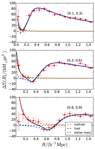
Figure 2: Observed galaxy-galaxy lensing signal for satellite galaxies as a function of the radius. The top, middle and bottom panels show results for satellites with $r_{p}$ in the range $[0.1,0.3]{\rm h^{-1}Mpc}$, $[0.3,0.6]{\rm h^{-1}Mpc}$ and $[0.6,0.9]{\rm h^{-1}Mpc}$, respectively. Red points with error bars represent the observational data. The vertical error bars show the 1 $\sigma$ bootstrap error. The horizontal error bars show the bin size. Black solid lines show the best-fit tNFW model prediction. Dashed lines of different colors show the contribution from the subhalo, the host halo, and the stellar mass respectively.

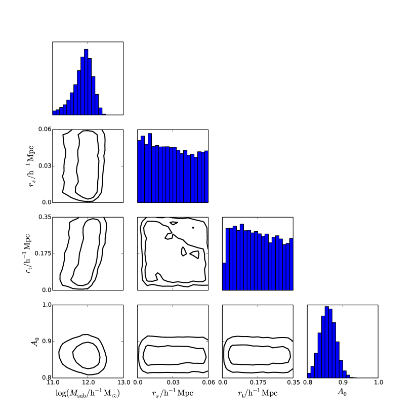
Figure 3: The contours show 68% and 95% confidence intervals for the tNFW model parameters, $M_{\rm sub}$, $r_{s}$, $r_{t}$ and $A_{0}$. Results are shown for satellites with $r_{p}=[0.3,0.6]{\rm h^{-1}Mpc}$. The last panel of each row shows the 1D marginalized posterior distributions. Note that the plotting range for $r_{s}$ and $r_{t}$ is exactly the same as the limits of our prior, so we actually do not have much constraints for these two parameters, except that high values are slightly disfavored for both.

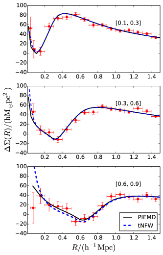
Figure 4: This figure is similar to Fig2. Solid lines represent the best-fit PIEMD model prediction and blue dashed lines are the predictions of the tNFW model.

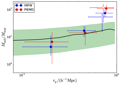
Figure 5: The subhalo mass-to-stellar mass ratio for galaxies in different $r_{p}$ bins. Vertical error bars show the 68% confidence interval. Empty circles show the best-fitted $M_{\rm sub}/M_{\rm star}$ values for $[0.6,0.9]{\rm h^{-1}Mpc}$ $r_{p}$ bin including the inner most observational point (see the bottom panel in Fig.2). Horizontal error bars show the bin range of $r_{p}$. The green shaded region represents the parameter space where 68% of the semi-analytical satellite galaxies distributes. The semi-analytical model also predicts an increasing $M_{\rm sub}/M_{\rm star}$ with $r_{p}$, but with a flatter slope.

Table 2: The best-fit values of the tNFW model parameters for the stacked satellite lensing signal in different $r_{p}$ bins. $\log{M_{\rm sub}}$, and $A_{\rm 0}$ are the best-fit values for the subhalo mass, and the normalization factor. We do not show the best-fit of $r_{s}$ and $r_{t}$ as they are poorly constrained. $N_{\rm sat}$ is the number of satellite galaxies in each bin. $\langle\log M_{\rm star}\rangle$ is the average stellar mass of satellites. All errors indicate the 68% confidence intervals. Masses are in units of $\rm{h^{-1}M_{\odot}}$. In our fiducial fitting process, we exclude the first point in $[0.6,0.9]{\rm h^{-1}Mpc}$ $r_{p}$ bin as a outlier (see Fig.2). For comparison, the bottom row of the table shows the fitting results including this first point.

$r_{p}$ range	$\langle\log(M_{\rm star})\rangle$	$\log{M_{\rm sub}}$	$A_{\rm 0}$	$M_{\rm sub}/M_{\rm star}$	$N_{\rm sat}$	$\langle z_{l}\rangle$
$[0.1,0.3]$	10.68	$11.37^{+0.35}_{-0.35}$	$0.80^{+0.01}_{-0.01}$	$4.43^{+6.63}_{-2.23}$	3963	0.33
$[0.3,0.6]$	10.72	$11.92^{+0.19}_{-0.18}$	$0.86^{+0.02}_{-0.02}$	$17.23^{+6.98}_{-6.84}$	2507	0.29
$[0.6,0.9]$	10.78	$12.64^{+0.12}_{-0.11}$	$0.81^{+0.04}_{-0.04}$	$75.40^{+19.73}_{-19.09}$	577	0.24
$[0.6,0.9]^{*}$	10.78	$12.49^{+0.13}_{-0.13}$	$0.81^{+0.04}_{-0.04}$	$54.64^{+15.58}_{-15.80}$	577	0.24

Table 3: best-fitted parameters with PIEMD model.

$r_{p}$ range	$\langle\log(M_{\rm star})\rangle$	$\log{M_{\rm sub}}$	$A_{\rm 0}$	$M_{\rm sub}/M_{\rm star}$
$[0.1,0.3]$	10.68	$11.30^{+0.55}_{-0.57}$	$0.80^{+0.01}_{-0.01}$	$6.72^{+7.84}_{-5.59}$
$[0.3,0.6]$	10.72	$11.76^{+0.33}_{-0.32}$	$0.86^{+0.01}_{-0.01}$	$14.40^{+9.01}_{-9.16}$
$[0.6,0.9]$	10.78	$12.80^{+0.15}_{-0.15}$	$0.79^{+0.04}_{-0.04}$	$110.98^{+35.76}_{-36.49}$
$[0.6,0.9]^{*}$	10.78	$12.84^{+0.13}_{-0.13}$	$0.79^{+0.04}_{-0.04}$	$119.74^{+34.34}_{-35.47}$

4.2 Dependence on satellite stellar mass

In the CDM structure formation scenario, satellite galaxies with larger stellar mass tend to occupy larger haloes at infall time (e.g. Vale & Ostriker, 2004; Conroy et al., 2006; Yang et al., 2012; Lu et al., 2014). In addition, massive haloes may retain more mass than lower mass ones at the same halo-centric radius (e.g. Conroy et al., 2006; Moster et al., 2010; Simha et al., 2012). For these two reasons, we expect that satellite galaxies with larger stellar mass reside in more massive subhalos.

To test this prediction, we select all galaxies with $r_{p}$ in the range $[0.3,0.9]$ ${\rm h^{-1}Mpc}$, and split the them into two subsamples: $10<\log(M_{\rm star}/\rm{h^{-1}M_{\odot}})<10.5$ and $11<\log(M_{\rm star}/\rm{h^{-1}M_{\odot}})<12$. The galaxy-galaxy lensing signals of the two satellite samples are shown in Fig.6. It is clear that at small scales, where subhalos dominate, the lensing signals are larger around the more massive satellites. The best-fit subhalo mass for the high mass and low mass satellites are $\log(M_{\rm sub}/\rm{h^{-1}M_{\odot}})=11.14^{+0.66}_{-0.73}$ ($M_{\rm sub}/M_{\rm star}=19.5^{+19.8}_{-17.9}$) and $\log(M_{\rm sub}/\rm{h^{-1}M_{\odot}})=12.38^{+0.16}_{-0.16}$ ($M_{\rm sub}/M_{\rm star}=21.1^{+7.4}_{-7.7}$ respectively.

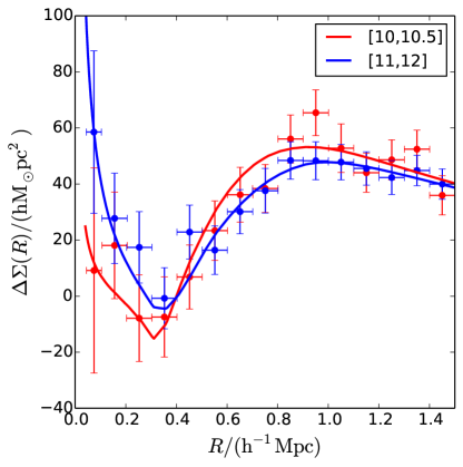
Figure 6: Observed galaxy-galaxy lensing signal for satellite galaxies in different stellar mass bins at fixed $r_{p}$. The legend shows the $\log(M_{\rm star}/\rm{h^{-1}M_{\odot}})$ range for different data points. The solid lines are the best-fit tNFW models.

5 Discussion and conclusion

In this paper, we present measurements of the galaxy-galaxy lensing signal of satellite galaxies in redMaPPer clusters. We select satellite galaxies from massive clusters (richness $\lambda>20$) in the redMaPPer catalog. We fit the galaxy-galaxy lensing signal around the satellites using a tNFW profile and a PIEMD profile, and obtain the subhalo masses. We bin satellite galaxies according to their projected halo-centric distance $r_{p}$ and find that the best-fit subhalo mass of satellite galaxies increases with $r_{p}$. The best-fit $\log({M_{\rm sub}/\rm{h^{-1}M_{\odot}}})$ for satellites in the $r_{p}=[0.6,0.9]{\rm h^{-1}Mpc}$ bin is larger than in the $r_{p}=[0.1,0.3]{\rm h^{-1}Mpc}$ bin by a factor of 18. The $M_{\rm sub}/M_{\rm star}$ ratio is also found to increase as a function of $r_{p}$ by a factor of 12. We also find that satellites with more stellar mass tend to populate more massive subhalos. Our results provide evidence for the tidal striping effects on the subhalos of red sequence satellite galaxies, as expected on the basis of the CDM hierarchical structure formation scenario.

Many previous studies have tried to test this theoretical prediction using gravitational lensing. Most of these previous studies focus on measuring subhalo mass in individual rich clusters. For example, Natarajan et al. (2009) report the measurement of dark matter subhalos as a function of projected halo-centric radius for the cluster C10024+16. They found that the mass of dark matter subhalos hosting early type $L^{*}$ galaxies increases by a factor of 6 from a halo-centric radius $r<0.6$ ${\rm h^{-1}Mpc}$ to $r\sim 4$ ${\rm h^{-1}Mpc}$. In recent work, Okabe et al. (2014) present the weak lensing measurement of 32 subhalos in the very nearby Coma cluster. They also found that the mass-to-light ratio of subhalos increase as a function of halo-centric radius: the $M/L_{\rm i^{\prime}}$ of subhalos increases from 60 at 10^′ to about 500 at 70^′.

Our work is complementary to these results. In the paper, we measure the galaxy-galaxy lensing signal of subhalos in a statistical sample of rich clusters. Our results lead to similar conclusions and show evidence for the effects of tidal striping. However, due to the statistical noise of the current survey, there is still a large uncertainties in the measurement of $M_{\rm sub}/M_{\rm star}$.

Theoretically, the galaxy - halo connection can be established by studying how galaxies of different properties reside in dark matter halos of different masses, through models such as the halo occupation models Jing et al. (e.g. 1998); Peacock & Smith (e.g. 2000); Berlind & Weinberg (e.g. 2002), the conditional luminosity functions models (e.g. Yang et al., 2003), (sub)halo-abundance-matching ( e.g. Vale & Ostriker, 2004; Conroy et al., 2006; Wang et al., 2006; Yang et al., 2012; Chaves-Montero et al., 2015), and empirical models of star formation and mass assembly of galaxies in dark matter halos (e.g. Lu et al., 2014, 2015). In most of these models, the connection is made between galaxy luminosities (stellar masses) and halo masses before a galaxy becomes a satellite, i.e. before a galaxy and its halo have experienced halo-specific environmental effects. The tidal stripping effects after a halo becomes a sub-halo can be followed in dark matter simulations. This, together with the halo-galaxy connection established through the various models, can be used to predict the subhalo - galaxy relation at the present day. During the revision of this paper, Han et al. (2016) posted a theoretical work on subhalo spatial and mass distributions. In Sec. 6.4 of their paper, they presented how our lensing measurements can be derived theoretically from a subhalo abundance matching point of view. With future data, the galaxy-galaxy lensing measurements of subhalos associated with satellites are expected to provide important constraints on galaxy formation and evolution in dark matter halos.

The results of this paper also demonstrate the promise of next generation weak lensing surveys. In Li et al. (2013), it is shown that the constraints on subhalo structures and $M_{\rm sub}/M_{\rm star}$ can be improved dramatically with next generation galaxy surveys such as LSST, due to the increase in both sky area (17000 deg²) and the depth (40 gal/arcmin²), which is crucial in constraining the co-evolution of satellite galaxies and subhalos. The space mission, such as Euclid, will survey a similar area of the sky (20000 deg²) but with much better image resolutions (FWHM $0.1"$ versus $0.7"$ for LSST), which is expected to provide even better measurements of galaxy-galaxy lensing. The method described here can readily be extended to these future surveys.

Appendix A Fake member contamination

The uncertainties of photometric redshifts cause the error in lens selection. The line-of-sight field galaxies may be misidentified as cluster members. These field galaxies are free of tidal disruption, causing an overestimation of the $M_{\rm sub}/M_{\rm star}$ for satellite galaxies. Rozo et al. (2015) investigate the cluster member identification, and find that the photometric membership estimator agrees with the spectroscopic membership with 1% precision. In this work, we use satellite galaxy with membership probability larger than 80%, which give us a mean probability of satellite $\sim 80\%-90\%$. Thus, we conclude that our satellite selection may face a 10%-15% contamination from the light sight field galaxies. According to Li et al. (2013), 10% interlopers contribute to about 15% of the total signal in the inner part. The accurate estimation of the contamination requires a detailed comparison with mock catalog constructed in proper simulations, which is not available at the moment. We thus made the following test to explore the effects of the interlopers. Instead of choosing satellite galaxies with $P_{\rm mem}>80\%$, we choose satellite galaxies with $P_{\rm mem}>60\%$, and re-calculate the lensing signal. We show the comparison of the lensing signal in Fig.7. The later $P_{\rm mem}$ selection will increase the interloper fraction from 10%-15% to 20%-25%. We find that the change in the lensing is only about 10% at the subhalo dominating region, smaller than the statistical error bars.

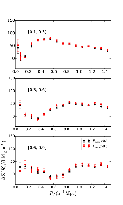
Figure 7: Observed galaxy-galaxy lensing signal for satellite galaxies with different $P_{\rm mem}$ selection.

Appendix B Photometric redshift bias test

The biased photometric redshifts can cause a systematic error in the measured lensing signal. We make the following test to explore this uncertainty. We split the source galaxy sample in two, the high-z ($z>0.7$) and the low-z ($z<0.7$) samples. We then compute $\Delta\Sigma(R)$ for the same set of lenses with each half of the sources. We fit $\Delta\Sigma_{high-z}=(1+b)\Delta\Sigma_{\rm low-z}$ where b is a free parameter, which is used to estimate the bias introduced by photo-z error. If the source redshifts are free from bias, we will have b=0. In this test, the lens sample can be any galaxies as long as their redshift distribution is the same with that of our satellite samples in the paper. To maximum the lensing signal, we thus select galaxies from the LOWZ and CMASS galaxies from SDSS-BOSS survey(Dawson et al., 2013), and require them to have the same redshift distribution as the satellite galaxies in our paper. The results are shown in Fig.8. We find that the b parameter is consistent with 0 within the statistical errors ($b=-0.05\pm 0.19$).

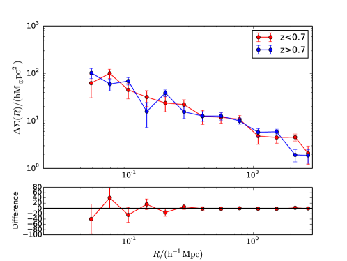
Figure 8: Observed galaxy-galaxy lensing signal with high-z sources (blue) and low-z sources (red). The lenses are selected from the LOWZ and CMASS galaxies. The lower panel shows the difference between results of the two sample of sources.

References

- Abadi et al. (1999) Abadi M. G., Moore B., Bower R. G., 1999, MNRAS, 308, 947
- Aihara et al. (2011) Aihara H., Allende Prieto C., An D., Anderson S. F., Aubourg É., Balbinot E., Beers T. C., 2011, ApJS, 195, 26
- Annis et al. (2014) Annis J., Soares-Santos M., Strauss M. A., Becker A. C., Dodelson S., Fan X., Gunn J. E., Hao J., Ivezić Ž., Jester S., Jiang L., Johnston D. E., Kubo J. M., Lampeitl H., Lin H., Lupton R. H., Miknaitis G., Seo H.-J., Simet M., Yanny B., 2014, ApJ, 794, 120
- Balogh et al. (2000) Balogh M. L., Navarro J. F., Morris S. L., 2000, ApJ, 540, 113
- Baltz et al. (2009) Baltz E. A., Marshall P., Oguri M., 2009, JCAP, 1, 15
- Benítez (2000) Benítez N., 2000, ApJ, 536, 571
- Berlind & Weinberg (2002) Berlind A. A., Weinberg D. H., 2002, ApJ, 575, 587
- Bose et al. (2016) Bose S., Hellwing W. A., Frenk C. S., Jenkins A., Lovell M. R., Helly J. C., Li B., 2016, MNRAS, 455, 318
- Bullock et al. (2001) Bullock J. S., Kolatt T. S., Sigad Y., Somerville R. S., Kravtsov A. V., Klypin A. A., Primack J. R., Dekel A., 2001, MNRAS, 321, 559
- Bundy et al. (2015) Bundy K., Leauthaud A., Saito S., Bolton A., Lin Y.-T., Marason C., Nichol R. C., Schneider D. P., Thomas D., Wake D. A., 2015, ArXiv e-prints
- Chabrier (2003) Chabrier G., 2003, PASP, 115, 763
- Chang et al. (2013) Chang J., Macciò A. V., Kang X., 2013, MNRAS, 431, 3533
- Chaves-Montero et al. (2015) Chaves-Montero J., Angulo R. E., Schaye J., Schaller M., Crain R. A., Furlong M., 2015, ArXiv e-prints
- Chung et al. (2009) Chung A., van Gorkom J. H., Kenney J. D. P., Crowl H., Vollmer B., 2009, AJ, 138, 1741
- Colín et al. (2000) Colín P., Avila-Reese V., Valenzuela O., 2000, ApJ, 542, 622
- Comparat et al. (2013) Comparat J., Jullo E., Kneib J.-P., Schimd C., Shan H., Erben T., Ilbert O., Brownstein J., Ealet A., Escoffier S., Moraes B., Mostek N., Newman J. A., Pereira M. E. S., Prada F., Schlegel D. J., Schneider D. P., Brandt C. H., 2013, MNRAS, 433, 1146
- Conroy et al. (2009) Conroy C., Gunn J. E., White M., 2009, ApJ, 699, 486
- Conroy et al. (2006) Conroy C., Wechsler R. H., Kravtsov A. V., 2006, ApJ, 647, 201
- Conroy et al. (2010) Conroy C., White M., Gunn J. E., 2010, ApJ, 708, 58
- Dawson et al. (2013) Dawson K. S., Schlegel D. J., Ahn C. P., Anderson S. F., Aubourg É., Bailey S., Barkhouser R. H., Bautista J. E., 2013, AJ, 145, 10
- De Lucia et al. (2004) De Lucia G., Kauffmann G., Springel V., White S. D. M., Lanzoni B., Stoehr F., Tormen G., Yoshida N., 2004, MNRAS, 348, 333
- Diemand et al. (2007) Diemand J., Kuhlen M., Madau P., 2007, ApJ, 657, 262
- Dolag et al. (2004) Dolag K., Bartelmann M., Perrotta F., Baccigalupi C., Moscardini L., Meneghetti M., Tormen G., 2004, A&A, 416, 853
- Duffy et al. (2008) Duffy A. R., Schaye J., Kay S. T., Dalla Vecchia C., 2008, MNRAS, 390, L64
- Erben et al. (2009) Erben T., Hildebrandt H., Lerchster M., Hudelot P., Benjamin J., van Waerbeke L., Schrabback T., Brimioulle F., 2009, A&A, 493, 1197
- Erben et al. (2013) Erben T., Hildebrandt H., Miller L., van Waerbeke L., Heymans C., Hoekstra H., Kitching T. D., Mellier Y., 2013, MNRAS, 433, 2545
- Frenk & White (2012) Frenk C. S., White S. D. M., 2012, Annalen der Physik, 524, 507
- Gao et al. (2011) Gao L., Frenk C. S., Boylan-Kolchin M., Jenkins A., Springel V., White S. D. M., 2011, MNRAS, 410, 2309
- Gao et al. (2012) Gao L., Navarro J. F., Frenk C. S., Jenkins A., Springel V., White S. D. M., 2012, MNRAS, 425, 2169
- Gao et al. (2004) Gao L., White S. D. M., Jenkins A., Stoehr F., Springel V., 2004, MNRAS, 355, 819
- George et al. (2012) George M. R., Leauthaud A., Bundy K., Finoguenov A., Ma C.-P., Rykoff E. S., Tinker J. L., Wechsler R. H., 2012, ApJ, 757, 2
- Gillis et al. (2013) Gillis B. R., Hudson M. J., Erben T., Heymans C., Hildebrandt H., Hoekstra H., Kitching T. D., Mellier 2013, MNRAS, 431, 1439
- Gunn & Gott (1972) Gunn J. E., Gott III J. R., 1972, ApJ, 176, 1
- Guo et al. (2011) Guo Q., White S., Boylan-Kolchin M., De Lucia G., Kauffmann G., Lemson G., Li C., Springel V., Weinmann S., 2011, MNRAS, 413, 101
- Han et al. (2016) Han J., Cole S., Frenk C. S., Jing Y., 2016, MNRAS, 457, 1208
- Han et al. (2015) Han J., Eke V. R., Frenk C. S., Mandelbaum R., Norberg P., Schneider M. D., Peacock J. A., Jing Y., Baldry I., Bland-Hawthorn J., Brough S., Brown M. J. I., Liske J., Loveday J., Robotham A. S. G., 2015, MNRAS, 446, 1356
- Hayashi et al. (2003) Hayashi E., Navarro J. F., Taylor J. E., Stadel J., Quinn T., 2003, ApJ, 584, 541
- Hellwing et al. (2015) Hellwing W. A., Frenk C. S., Cautun M., Bose S., Helly J., Jenkins A., Sawala T., Cytowski M., 2015, ArXiv e-prints
- Heymans et al. (2012) Heymans C., Van Waerbeke L., Miller L., Erben T., Hildebrandt H., Hoekstra H., Kitching T. D., Mellier Y., 2012, MNRAS, 427, 146
- Jing et al. (1998) Jing Y. P., Mo H. J., Börner G., 1998, ApJ, 494, 1
- Kang & van den Bosch (2008) Kang X., van den Bosch F. C., 2008, ApJL, 676, L101
- Kassiola & Kovner (1993) Kassiola A., Kovner I., 1993, ApJ, 417, 450
- Kawata & Mulchaey (2008) Kawata D., Mulchaey J. S., 2008, ApJL, 672, L103
- Klimentowski et al. (2007) Klimentowski J., Łokas E. L., Kazantzidis S., Prada F., Mayer L., Mamon G. A., 2007, MNRAS, 378, 353
- Kneib et al. (1996) Kneib J.-P., Ellis R. S., Smail I., Couch W. J., Sharples R. M., 1996, ApJ, 471, 643
- Kneib & Natarajan (2011) Kneib J.-P., Natarajan P., 2011, A&ARv, 19, 47
- Komatsu et al. (2010) Komatsu E., Smith K. M., Dunkley J., Bennett C. L., Gold B., Hinshaw G., Jarosik N., Larson D., 2010, ArXiv e-prints
- Koopmans (2005) Koopmans L. V. E., 2005, MNRAS, 363, 1136
- Lang et al. (2014) Lang D., Hogg D. W., Schlegel D. J., 2014, ArXiv e-prints
- Li et al. (2009) Li R., Mo H. J., Fan Z., Cacciato M., van den Bosch F. C., Yang X., More S., 2009, MNRAS, 394, 1016
- Li et al. (2013) Li R., Mo H. J., Fan Z., Yang X., Bosch F. C. v. d., 2013, MNRAS, 430, 3359
- Li et al. (2014) Li R., Shan H., Mo H., Kneib J.-P., Yang X., Luo W., van den Bosch F. C., Erben T., Moraes B., Makler M., 2014, MNRAS, 438, 2864
- Limousin et al. (2007) Limousin M., Kneib J. P., Bardeau S., Natarajan P., Czoske O., Smail I., Ebeling H., Smith G. P., 2007, A&A, 461, 881
- Limousin et al. (2005) Limousin M., Kneib J.-P., Natarajan P., 2005, MNRAS, 356, 309
- Limousin et al. (2009) Limousin M., Sommer-Larsen J., Natarajan P., Milvang-Jensen B., 2009, ApJ, 696, 1771
- Lu et al. (2014) Lu Z., Mo H. J., Lu Y., Katz N., Weinberg M. D., van den Bosch F. C., Yang X., 2014, MNRAS, 439, 1294
- Lu et al. (2015) Lu Z., Mo H. J., Lu Y., Katz N., Weinberg M. D., van den Bosch F. C., Yang X., 2015, MNRAS, 450, 1604
- Macciò et al. (2007) Macciò A. V., Dutton A. A., van den Bosch F. C., Moore B., Potter D., Stadel J., 2007, MNRAS, 378, 55
- Mandelbaum et al. (2005) Mandelbaum R., Hirata C. M., Seljak U., Guzik J., Padmanabhan N., Blake C., Blanton M. R., Lupton R., Brinkmann J., 2005, MNRAS, 361, 1287
- Mandelbaum et al. (2008) Mandelbaum R., Seljak U., Hirata C. M., 2008, JCAP, 8, 6
- Mao et al. (2004) Mao S., Jing Y., Ostriker J. P., Weller J., 2004, ApJL, 604, L5
- Mao & Schneider (1998) Mao S., Schneider P., 1998, MNRAS, 295, 587
- Mayer et al. (2001) Mayer L., Governato F., Colpi M., Moore B., Quinn T., Wadsley J., Stadel J., Lake G., 2001, ApJL, 547, L123
- McCarthy et al. (2008) McCarthy I. G., Frenk C. S., Font A. S., Lacey C. G., Bower R. G., Mitchell N. L., Balogh M. L., Theuns T., 2008, MNRAS, 383, 593
- Metcalf & Madau (2001) Metcalf R. B., Madau P., 2001, ApJ, 563, 9
- Miller et al. (2013) Miller L., Heymans C., Kitching T. D., van Waerbeke L., Erben T., Hildebrandt H., Hoekstra H., Mellier Y., 2013, MNRAS, 429, 2858
- Miller et al. (2007) Miller L., Kitching T. D., Heymans C., Heavens A. F., van Waerbeke L., 2007, MNRAS, 382, 315
- Miyatake et al. (2013) Miyatake H., More S., Mandelbaum R., Takada M., Spergel D. N., Kneib J.-P., Schneider D. P., Brinkmann J., Brownstein J. R., 2013, ArXiv e-prints
- Moster et al. (2010) Moster B. P., Somerville R. S., Maulbetsch C., van den Bosch F. C., Macciò A. V., Naab T., Oser L., 2010, ApJ, 710, 903
- Moustakas et al. (2013) Moustakas J., Coil A. L., Aird J., Blanton M. R., Cool R. J., Eisenstein D. J., Mendez A. J., Wong K. C., Zhu G., Arnouts S., 2013, ApJ, 767, 50
- Natarajan et al. (2007) Natarajan P., De Lucia G., Springel V., 2007, MNRAS, 376, 180
- Natarajan et al. (2009) Natarajan P., Kneib J.-P., Smail I., Treu T., Ellis R., Moran S., Limousin M., Czoske O., 2009, ApJ, 693, 970
- Navarro et al. (1997) Navarro J. F., Frenk C. S., White S. D. M., 1997, ApJ, 490, 493
- Neto et al. (2007) Neto A. F., Gao L., Bett P., Cole S., Navarro J. F., Frenk C. S., White S. D. M., Springel V., Jenkins A., 2007, MNRAS, 381, 1450
- Nierenberg et al. (2014) Nierenberg A. M., Treu T., Wright S. A., Fassnacht C. D., Auger M. W., 2014, MNRAS, 442, 2434
- Oguri & Hamana (2011) Oguri M., Hamana T., 2011, MNRAS, 414, 1851
- Okabe et al. (2014) Okabe N., Futamase T., Kajisawa M., Kuroshima R., 2014, ApJ, 784, 90
- Pastor Mira et al. (2011) Pastor Mira E., Hilbert S., Hartlap J., Schneider P., 2011, A&A, 531, A169
- Peacock & Smith (2000) Peacock J. A., Smith R. E., 2000, MNRAS, 318, 1144
- Rozo & Rykoff (2014) Rozo E., Rykoff E. S., 2014, ApJ, 783, 80
- Rozo et al. (2015) Rozo E., Rykoff E. S., Becker M., Reddick R. M., Wechsler R. H., 2015, MNRAS, 453, 38
- Rykoff et al. (2012) Rykoff E. S., Koester B. P., Rozo E., Annis J., Evrard A. E., Hansen S. M., Hao J., Johnston D. E., McKay T. A., Wechsler R. H., 2012, ApJ, 746, 178
- Rykoff et al. (2014) Rykoff E. S., Rozo E., Busha M. T., Cunha C. E., Finoguenov A., Evrard A., Hao J., Koester B. P., Leauthaud A., Nord B., Pierre M., Reddick R., Sadibekova T., Sheldon E. S., Wechsler R. H., 2014, ApJ, 785, 104
- Salpeter (1955) Salpeter E. E., 1955, ApJ, 121, 161
- Shan et al. (2015) Shan H., Kneib J.-P., Li R., Comparat J., Erben T., Makler M., Moraes B., Van Waerbeke L., Taylor J. E., Charbonnier A., 2015, ArXiv e-prints
- Shirasaki (2015) Shirasaki M., 2015, ApJ, 799, 188
- Sifón et al. (2015) Sifón C., Cacciato M., Hoekstra H., Brouwer M., van Uitert E., Viola M., Baldry I., Brough S., 2015, ArXiv e-prints
- Simha et al. (2012) Simha V., Weinberg D. H., Davé R., Fardal M., Katz N., Oppenheimer B. D., 2012, MNRAS, 423, 3458
- Springel et al. (2006) Springel V., Frenk C. S., White S. D. M., 2006, Nature, 440, 1137
- Springel et al. (2008) Springel V., Wang J., Vogelsberger M., Ludlow A., Jenkins A., Helmi A., Navarro J. F., Frenk C. S., 2008, MNRAS, 391, 1685
- Springel et al. (2001) Springel V., White S. D. M., Tormen G., Kauffmann G., 2001, MNRAS, 328, 726
- Taffoni et al. (2003) Taffoni G., Mayer L., Colpi M., Governato F., 2003, MNRAS, 341, 434
- Tormen et al. (1998) Tormen G., Diaferio A., Syer D., 1998, MNRAS, 299, 728
- Vale & Ostriker (2004) Vale A., Ostriker J. P., 2004, MNRAS, 353, 189
- Vegetti & Koopmans (2009a) Vegetti S., Koopmans L. V. E., 2009a, MNRAS, 392, 945
- Vegetti & Koopmans (2009b) Vegetti S., Koopmans L. V. E., 2009b, MNRAS, 400, 1583
- Vegetti et al. (2010) Vegetti S., Koopmans L. V. E., Bolton A., Treu T., Gavazzi R., 2010, MNRAS, 408, 1969
- Vegetti et al. (2012) Vegetti S., Lagattuta D. J., McKean J. P., Auger M. W., Fassnacht C. D., Koopmans L. V. E., 2012, Nature, 481, 341
- Wang et al. (2006) Wang L., Li C., Kauffmann G., De Lucia G., 2006, MNRAS, 371, 537
- Wang et al. (2007) Wang L., Li C., Kauffmann G., De Lucia G., 2007, MNRAS, 377, 1419
- Wetzel et al. (2013) Wetzel A. R., Tinker J. L., Conroy C., van den Bosch F. C., 2013, MNRAS, 432, 336
- Wright et al. (2010) Wright E. L., Eisenhardt P. R. M., Mainzer A. K., Ressler M. E., Cutri R. M., Jarrett T., Kirkpatrick J. D., 2010, AJ, 140, 1868
- Xie & Gao (2015) Xie L., Gao L., 2015, MNRAS, 454, 1697
- Xu et al. (2009) Xu D. D., Mao S., Wang J., Springel V., Gao L., White S. D. M., Frenk C. S., Jenkins A., Li G., Navarro J. F., 2009, MNRAS, 398, 1235
- Yang et al. (2003) Yang X., Mo H. J., van den Bosch F. C., 2003, MNRAS, 339, 1057
- Yang et al. (2006) Yang X., Mo H. J., van den Bosch F. C., Jing Y. P., Weinmann S. M., Meneghetti M., 2006, MNRAS, 373, 1159
- Yang et al. (2007) Yang X., Mo H. J., van den Bosch F. C., Pasquali A., Li C., Barden M., 2007, ApJ, 671, 153
- Yang et al. (2012) Yang X., Mo H. J., van den Bosch F. C., Zhang Y., Han J., 2012, ApJ, 752, 41
- Zhao et al. (2003) Zhao D. H., Jing Y. P., Mo H. J., Börner G., 2003, ApJL, 597, L9
- Zhao et al. (2009) Zhao D. H., Jing Y. P., Mo H. J., Börner G., 2009, ApJ, 707, 354