Rigorous numerics for fast-slow systems with one-dimensional slow variable: topological shadowing approach
Abstract
We provide a rigorous numerical computation method to validate periodic, homoclinic and heteroclinic orbits as the continuation of singular limit orbits for the fast-slow system
with one-dimensional slow variable . Our validation procedure is based on topological tools called isolating blocks, cone condition and covering relations. Such tools provide us with existence theorems of global orbits which shadow singular orbits in terms of a new concept, the covering-exchange. Additional techniques called slow shadowing and -cones are also developed. These techniques give us not only generalized topological verification theorems, but also easy implementations for validating trajectories near slow manifolds in a wide range, via rigorous numerics. Our procedure is available to validate global orbits not only for sufficiently small but all in a given half-open interval . Several sample verification examples are shown as a demonstration of applicability.
Keywords: singular perturbations, periodic orbits, connecting orbits, rigorous numerics, covering-exchange.
AMS subject classifications : 34E15, 37B25, 37C29, 37C50, 37D10, 65L11
1 Introduction
1.1 Background of problems and our aims
In this paper, we consider the dynamical system in of the following form:
| (1.1) |
where is the time derivative and are -functions with . The factor is a nonnegative but sufficiently small real number. We shall write (1.1) as (1.1)ϵ if we explicitly represent the -dependence of the system. The system (1.1) can be reformulated with a change of time-scale variable as
| (1.2) |
where and . One tries to analyze the dynamics of (1.1), equivalently (1.2), by suitably combining the dynamics of the layer problem
| (1.3) |
and the dynamics of the reduced problem
| (1.4) |
which are the limiting problems for on the fast and the slow time scale, respectively. Notice that (1.4) makes sense only on , while (1.3) makes sense in whole as the -parameter family of -systems. The meaning of the “-limit” is thus different between (1.1) and (1.2). This is why (1.1) or (1.2) is a kind of singular perturbation problems. In particular, (1.1) or (1.2) is known as fast-slow systems (or slow-fast systems), where dominates the behavior in the fast time scale and dominates the behavior in the slow time scale.
When we study the dynamical system of the form (1.1), we often consider limit systems (1.3) and (1.4) independently at first. Then ones try to match them in an appropriate way to obtain trajectories for the full system (1.1). One of major methods for completely solving singularly perturbed systems like (1.1) is the geometric singular perturbation theory formulated by Fenichel [10], Jones-Kopell [20], Szmolyan [32] and many researchers. A series of theories are established so that formally constructed singular limit orbits of (1.3) and (1.4) can perturb to true orbits of (1.1) for sufficiently small . In geometric singular perturbation theory, there are mainly two key points to consider. One is the description of slow dynamics for sufficiently small near the nullcline . The other is the matching of fast and slow dynamics. As for the former, Fenichel [10] provided the Invariant Manifold Theorem for describing the dynamics on and around locally invariant manifolds, called slow manifolds, for sufficiently small . Such manifolds can be realized as the perturbation of normally hyperbolic invariant manifolds at , which are often given by submanifolds of nullcline in (1.3). As for the latter, Jones and Kopell [20] originally formulated the geometric answer for the matching problem deriving Exchange Lemma. This lemma informs that the manifold configuration upon exit from the neighborhood of slow manifolds under the assumption of transversal intersection between tracking invariant manifolds and the stable manifold of slow manifolds. Afterwards, Exchange Lemma has been extended in various directions, e.g. [19, 22, 33]. Combining these terminologies, one can prove the existence of homoclinic or heteroclinic orbits of invariant sets near singular orbits for sufficiently small . There are also topological ways to prove their existence for sufficiently small provided by, say, Carpenter [4], Gardner-Smoller [12] and so on, by using algebraic-topological concepts such as the mapping degree or the Conley index [7, 25]. Such topological approaches also mention the existence of periodic orbits near singular orbits.
On the other hand, all such mathematical results do not give us how large such sufficiently small is. In other words, it remains an open problem whether there exist global orbits given by the continuation of singular orbits for a given . This intrinsic problem has been mentioned in many discussions (e.g. [17]). From the viewpoint of numerical computations, if is sufficiently small, (1.1) becomes the stiff problem and numerically unstable. Although the effective method for computing slow manifolds is provided by Guchenheimer and Kuehn [16], computations for extremely small (e.g. close to machine epsilon) is still hard to operate correctly. These circumstances show that there are gaps between mathematical results (i.e. sufficiently small ) and numerical observations (i.e. given ) for completely understanding dynamics of fast-slow systems. These are mainly because there are no estimations to measure mathematically rigorous consequences not only quantitatively but also qualitatively. The construction of procedures which bridge mathematical results and numerical observations is necessary to completely understand phenomena in concrete dynamical systems, which is also the case of singular perturbation problems.
Our main aim in this paper is to provide implementations for validating the continuation of various global orbits of (1.1) for all rigorously, where is a given number. In other words, we provide a method to validate
- (Main 1)
-
the singular limit orbit for (1.1) with , as well as
- (Main 2)
-
global orbits near for all for a given .
Singular limit orbit means the union of several heteroclinic orbits in (1.3) and the submanifolds of the nullcline . Global orbits mean homoclinic, heteroclinic orbits of invariant sets and periodic orbits.
To this end, we provide the notion of covering-exchange, which is a topological analogue of Exchange Lemma. This concept consists of the following topological notions with suitable assumptions: (i) isolating blocks, (ii) cone conditions and (iii) covering relations. These three notions have been already applied to validations of global orbits in dynamical systems very well, as stated in Section 1.2. The covering-exchange is constructed by those notions, and informs us
- •
-
•
the existence of trajectories not only which converge to invariant sets on slow manifolds but also which exits neighborhoods of slow manifolds after time .
These properties and the general consequence of covering relations yield the existence of global orbits. We also generalize the covering-exchange by introducing the additional notion of slow shadowing, which guarantees the local existence of trajectories which shadow slow manifolds with nonlinear structure. This notion enables us to trace trajectories which not only tend to slow manifolds but also stay near slow manifolds for time from topological viewpoints. This concept is also very compatible with numerical computations, in particular, for validating trajectories near slow manifolds.
The other main tool to establish our procedure is the assistance of rigorous numerics, namely, computations of enclosures where mathematically correct objects are contained in the phase space. All such computations can be realized by interval arithmetics and mathematical error estimates. Combination of the covering-exchange, slow shadowing and rigorous numerics in reasonable processes provide us with a method proving (Main 1) and (Main 2) simultaneously.
Note that there are two approaches to consider singular perturbation problems; one is the continuation of structures from the singular limit systems () to the full systems (i.e. ), and the other is the consideration of full systems to the singular limit . Our attitude is the former. In particular, we consider our problems via topological approach on the basis of geometric singular perturbation theory.
This paper is organized as follows. In Section 2, we briefly review Fenichel’s invariant manifold theorem and topological notions called covering relations and isolating blocks. A systematic procedure of isolating blocks for validations of invariant manifolds with computer assistance (e.g. [42, 23]) is also discussed.
In Section 3, we show how slow manifolds can be validated in given regions with an explicit range of . One sees that our fundamental arguments are basically followed by the proof in Jones’ article [18]. Such arguments can be validated via the construction of isolating blocks and singular perturbation problems’ version of cone conditions (cf. [39]) and Lyapunov condition [23].
In Section 4, we discuss treatments of slow dynamics. First we introduce the new notion called the covering-exchange for describing the behavior of trajectories around slow manifolds (Section 4.1). This concept is a topological analogue of Exchange Lemma so that we can reasonably validate tracking invariant manifolds near slow manifolds in a suitable sense. This concept also solves the matching problem between fast and slow dynamics. We also provide a generalization of the covering-exchange; a collection of local behavior near slow manifolds called slow shadowing, drop and jump (Section 4.3). These concepts enable us to construct true trajectories in full system which shadow ones on slow manifolds in reasonable ways via rigorous numerics. Furthermore, we provide a slight extension of cones, called -cones, which enables us to sharpen enclosures of stable and unstable manifolds of normally hyperbolic invariant manifolds (Section 4.4). The main idea itself is just a slight modification of cone conditions stated in Section 3. But this technique gives us a lot of benefits in many scenes incorporating with rigorous numerics. On the other hand, dynamics on slow manifolds should be considered when slow manifolds exhibit the nontrivial dynamics such as fixed points, periodic orbits, homoclinic orbits, etc. As an example, we discuss validations of nontrivial fixed points on slow manifolds (Section 4.5). In the end of Section 4, we discuss unstable manifolds of invariant sets on slow manifolds (Section 4.6). To deal with these manifolds, we discuss the invariant foliations of slow manifolds, and translate this fiber bundle structure into the terms of cones and covering relations. This is one of key considerations of heteroclinic orbits in (1.1)ϵ.
In Section 5, the existence theorems for periodic and heteroclinic orbits near singular limit orbits with an explicit range of are presented.
As demonstrations of our proposing implementations, we study the FitzHugh-Nagumo equation:
| (1.5) |
where , and .
The existence of global orbits such as periodic or homoclinic orbits for sufficiently small are widely discussed by many authors (e.g. [4, 12]). Note that, as we mentioned before, the existence of those orbits for a given remains an open question. Our proposing ideas lead a road to answer this question.
Computer Assisted Result 1.1 (Existence of homoclinic orbits).
Consider (1.5) with , and . Then for all , there exist the following two kinds of trajectories:
-
1.
At , a singular heteroclinic chain consisting of
-
•
heteroclinic orbit from the equilibrium near to the equilibrium near ,
-
•
heteroclinic orbit from the equilibrium near to the equilibrium near , and
-
•
two branches of nullcline connecting two heteroclinic orbits.
-
•
-
2.
For all , a homoclinic orbit of near .
The precise statements and other sample validation results are shown in Section 6. Throughout the rest of this paper we make the following assumption, which is essential to our whole discussions herein.
Assumption 1.2.
Vector fields and have the following form:
General dynamical systems depend on parameters. For example, the FitzHugh-Nagumo system (1.5) contains as parameters. Throughout this paper we do not care about parameter dependence of dynamical systems unless otherwise specified.
1.2 Several preceding works related to global trajectories and singular perturbation problems with rigorous numerics
There are many preceding works for the existence of global orbits with rigorous numerics for regular dynamical systems, namely, case. For example, Wilczak and Zgliczyński [37] apply the topological tool called covering relations to the existence of various type of trajectories in dynamical systems, such as periodic orbits, homoclinic orbits and heteroclinic orbits. The essence of covering relations is to describe behavior of rectangular-like sets called -sets and apply the mapping degree to the existence of solutions. One of powerful properties of covering relations is that every -sets can be used as a joint of trajectories and that we can validate various complicating behavior of dynamical systems. Indeed, for example, [35] and [36] by Wilczak validate various type of complex trajectories such as Shi’lnikov homoclinic solutions, heteroclinic solutions and infinitely many periodic solutions in concrete systems (e.g. Michelson system or Rössler system).
On the other hand, van der Berg et. al. [34] produce the other approach of rigorous numerical computations of connecting orbits using radii polynomials and parametrization technique. Their main idea is to reduce the original problem to a projected boundary value problem in an infinite dimensional functional space via a fixed point argument. Their formulation involves a higher order parametrization of invariant manifolds near equilibria for describing stable and unstable manifolds. Their approach is free from integrations of vector fields. Hence one can validate various additional properties of invariant manifolds without any knowledges of the existence of trajectories [5].
As for rigorous numerics for singular perturbation problems, Gameiro et. al. [11] provide a validation method combined with the algebraic-topological singular perturbation analysis. Such analysis is knows as the Conley index theory [7, 25]. They actually apply its singular perturbation version [14, 13] to the singularly perturbed predetor-prey model with two slow variables. As a result, they prove the existence of topological horseshoe, in particular, infinite number of periodic orbits with computer assistance. Their results show, however, the existence of solutions for only sufficiently small and hence the bound of where the existence result holds is not given. When we apply the Conley index technique, it is necessary to provide an appropriate neighborhood of desiring orbits whose boundary transversally intersects the vector field defined by the full system (1.1).
On the other hand, Guckenheimer et. al. [15] discusses rigorous enclosures of slow manifolds with computer assistance within explicit ranges of . They introduce a concept of computational slow manifolds related to slow manifolds in geometric singular perturbation theory and succeed validations of slow manifolds in their settings with in explicit ranges of , while validated ranges of are bounded away from , say, . Note that [15] also discusses validations of tangential bifurcations of slow manifolds for all , where is a given number, say, . One of the other works is a very recent one by Arioli and Koch [1], which studies the existence and the stability of traveling pulse solutions for the (singularly perturbed) FitzHugh-Nagumo system. This study, however, focuses only for the parameter range which is not so small, say, or . In other words, the singular perturbation structure is ignored.
In the case of singular perturbation problems, direct computations of global orbits without any ideas are not practical in various scenes both in the rigorous and in the non-rigorous sense.
Direct applications of such preceding works without any modifications would yield the failure of operations if we try to cover not only which is not so small (e.g. or ) but also extremely small , possibly smaller than machine epsilon. This failure is because either the stiffness of problems or the effect of fast dynamics. Even if it succeeds, there would be huge computation costs due to very slow behavior around slow manifolds. Of course, there is a matching problem connecting fast and slow behavior, which is generally arisen in singular perturbation problems. If we can overcome all such difficulties as simple as possible, the scope of applications of preceding concepts will dramatically extend.
2 Preliminaries
When we consider a fast-slow system (1.1) from the viewpoint of geometric singular perturbation theory following Fenichel (e.g. [10]), the central issue is normally hyperbolic invariant manifolds. Fenichel’s theory tells us very rich structure of normally hyperbolic invariant manifolds consisting of equilibria and their small perturbations. Such structures are fully applied to our arguments. In the beginning of this section, we review several results about normally hyperbolic invariant manifolds for fast-slow systems.
Our main methodologies to consider fast-slow systems are well-known topological tools called covering relations, isolating blocks and cone conditions. These tools well describe behavior of solution sets as well as their asymptotic behavior. In successive sections we see that these tools work well even for fast-slow systems. In this section, we also review two of such tools. We also provide a procedure of isolating blocks suitable for fast-slow systems so that they validate slow manifolds, which are available to various systems with computer assistance. Cone conditions for singular perturbation problems are stated later.
Finally note that readers who are familiar with these topics can skip this section.
2.1 Fenichel’s Invariant Manifold Theorems : review
Here we briefly review the Fenichel’s Invariant Manifold Theorems (e.g. [10]), following arguments in [18]. The central goal of these results is the description of flow near the set with manifold structures: the critical manifold. The critical manifold can be considered as the -parameter family of equilibria of the layer problem (1.3). Under appropriate hypotheses, can be represented by the graph of a function for , where is a compact, simply connected set.
A central assumption among Fenichel’s theory is the normal hyperbolicity and the graph representation of .
- (F)
-
The set is given by the graph of the function for , where the set is a compact, simply connected domain whose boundary is an -dimensional submanifold. Moreover, assume that is normally hyperbolic.
Remark 2.1 (cf. [18]).
Recall that the manifold is normally hyperbolic if the linearization of (1.3) at each point in has exactly eigenvalues on the imaginary axis.
A set is said to be locally invariant under the flow generated by (1.1) if it has a neighborhood of so that no trajectory can leave without also leaving . In other words, it is locally invariant if for all , then implies that , similarly with replaced by when , where is a flow.
Without the loss of generality, we can assume that for all . Then, there exist the stable and unstable eigenspaces, and , such that and hold for all . With this in mind, we take the transformation so that (1.1) is expressed by
| (2.1) |
Here denotes the matrix which all eigenvalues have positive real part and denotes the matrix which all eigenvalues have negative real part. and denotes the higher order term which admit a positive number satisfying
More precise assumptions for and are as follows: there exist the quantities and such that
| (2.2) | |||
| (2.3) |
The key consideration of slow manifolds is the following Fenichel’s invariant manifold theorem in terms of graph representations.
Proposition 2.2 (Persistence of invariant manifolds. cf. [18]).
Under the assumption (F), for sufficiently small , there is a function defined on . The graph is locally invariant under (1.1). Moreover is , for any , jointly in and .
Proposition 2.2 is just a consequence of the second Invariant Manifold Theorem as follows.
Proposition 2.3 (Stable and unstable manifolds. cf. [18]).
Under the assumption (F), for sufficiently small , then for some ,
Fenichel’s theorems, Propositions 2.2 and 2.3, insist that normally hyperbolic invariant manifolds as well as their stable and unstable manifolds persist to locally invariant manifolds in the full system (1.1) for sufficiently small . In other words, slow manifolds can be realized by the -continuation of normally hyperbolic critical manifolds in the layer problem (1.3). The perturbed manifold for is called a slow manifold. One of strategies for constructing such manifolds is the construction of a family of isolating blocks and moving cones ([18]). Isolating blocks describe the behavior of vector fields which are transversal to their boundaries, which are well discussed in the Conley index theory [7, 25]. Isolating blocks are reviewed in Section 2.3.
Fenichel’s invariant manifold theory informs us not only the existence of perturbed slow manifolds but also invariant foliations of and . More precisely, the following result (the third Invariant Manifold Theorem) is known.
Proposition 2.4 (Fenichel fibering, cf. Theorem 6, 7 in [18]).
Under the assumption (F), for sufficiently small the following statements hold. For each ,
-
1.
there is a function for sufficiently small so that the graph
forms a locally invariant manifold in the sense that holds if for all . Here the set denotes the forward evolution of a set restricted to given by
Moreover, is in and jointly for any .
-
2.
there is a function for sufficiently small so that the graph
forms a locally invariant manifold in the sense that holds if for all . Moreover, is in and jointly for any .
This invariant foliation is sometimes referred to as Feniciel fibering. This fibering ensures us the following representations:
where is a subset of slow manifolds.
2.2 Covering relations : review
Our main approach to tracking solution orbits is a topological tool called covering relations. Covering relations describe topological transversality of rectangular-like domains called -sets relative to continuous map, and there are various studies not only from the mathematical viewpoint but also for applications with rigorous numerics (e.g. [3, 35, 37, 39, 41]). In the present study, we apply this topological methodology to singular perturbation problems. In this section, we summarize notions among the theory of covering relations. For a given norm on , let be the open ball of radius centered at . For simplicity, also let . We set , and .
Definition 2.5 (-set, cf. [39, 41]).
An -set consists of the following set, integers and a map:
-
•
A compact subset .
-
•
Nonnegative integers and such that with .
-
•
A homeomorphism satisfying
Finally define the dimension of an -set by .
We shall write an -set simply by if no confusion arises. Let
The following notion describes the topological transversality between two -sets relative to continuous maps.
Definition 2.6 (Covering relations, cf. [39, 41]).
Let be -sets with and . denotes a continuous mapping and . We say -covers () if the following statements hold:
-
1.
There exists a continuous homotopy satisfying
where ().
-
2.
There exists a mapping such that
(2.4) holds for .
Remark 2.7.
In definition of covering relation between and , the disagreement of and is not essential. On the contrary, the equality is essential because the mapping degree of -dimensional mapping should be derived.
The following propositions gives us useful sufficient conditions for detecting covering relations in practical situations.
Proposition 2.8 (Finding covering relations, Theorem 15 in [41]).
Let be two -sets in such that and . Let be continuous. Let . Assume that there exists such that following conditions are satisfied:
-
1.
Setting ,
-
2.
Define a map by
where be the orthogonal projection onto , . Assume that
Then .
Proposition 2.9 (Covering relation in the case , Definition 10 in [40]).
Let be -sets with . Let be continuous. Set
Assume that there exists such that
and either of the following conditions holds:
Then .
We also consider covering relations with respect to the inverse of continuous maps.
Definition 2.10 (Back-covering relation, Definition 3 and 4 in [41]).
Let be an -set. Define the -set as follows:
-
•
The compact subset of the quadruple is itself.
-
•
, .
-
•
The homeomorphism is given by
where is given by .
Notice that and .
Next, let be -sets such that . Let . Assume that is well-defined and continuous. Then we say -back-covers () if holds.
A fundamental result in the theory of covering relations is the following proposition.
Proposition 2.11 (Theorem 4 in [41]).
Let be -sets such that for and let , , be continuous. Assume that, for all , either of the following holds:
or
Then there is a point such that
If we additionally assume , then the point can be chosen so that
We sometimes consider an infinite sequence of covering relations. To deal with such a situation, we define the following concept.
Definition 2.12 (Admissibility, cf. Definition 2.4 in [35]).
Let be -sets in and be a continuous map. We say the index sequence is admissible with respect to if holds of all . Similarly, we say the index sequence is back-admissible with respect to if holds of all . In this case, is assumed to be well-defined in a neighborhood of and continuous.
Recall that the second Invariant Manifold Theorem, Proposition 2.3, claims that the stable and unstable manifolds of normally hyperbolic invariant manifolds can be described by graphs of smooth functions. The concept of horizontal and vertical disks are useful to describe asymptotic trajectories in terms of covering relations for describing these situations.
Definition 2.13 (Horizontal and vertical disk, e.g. [35, 39]).
Let be an -set. Let be continuous and let . We say that is a vertical disk in if there exists a homotopy such that
Let be continuous and let . We say that is a horizontal disk in if there exists a homotopy such that
Combining these concepts with covering relations, we obtain the following result, which is often applied to the existence of homoclinic and heteroclinic orbits.
2.3 Isolating blocks : review and applications to fast-slow systems
A concept of isolating blocks are typically discussed in the Conley index theory (e.g. [7, 25]), which studies the structure of isolated invariant sets from the algebraic-topological viewpoint. Central notions are isolating neighborhoods or index pairs in the Conley index theory, but we concentrate our attentions on isolating blocks defined as follows. In our case, the blocks can be considered very flexible from the viewpoint of not only covering relations but also rigorous numerics. Moreover, isolating blocks play central roles for the existence of slow manifolds (cf. [18] and Section 3). In this section, we firstly review the definition of isolating blocks. Secondly, we show a procedure of isolating blocks around equilibria and their alternatives for fast-slow systems with computer assistance, following [42].
2.3.1 Definition
Definition 2.15 (Isolating block).
Let be a compact set. We say an isolating neighborhood if holds, where
for a flow on . Next let be a compact set and . We say an exit (resp. entrance) point of , if for every solution through , with and there are and such that for ,
and for ,
hold. (resp. ) denote the set of all exit (resp. entrance) points of the closed set . We call and the exit and the entrance of , respectively. Finally is called an isolating block if holds and is closed in .
Obviously, an isolating block is also an isolating neighborhood.
2.3.2 Construction around equilibria via rigorous numerics : a basic form
There is a preceding work for the systematic construction of isolating blocks around equilibria [42]. Here we briefly review the method therein keeping the fast-slow system (1.1) in mind. The first part is the review of the preceding work [42]. As the second part, we discuss the analogue of arguments to fast-slow systems. One will see that such procedures are very suitable for analyzing dynamics around invariant manifolds.
Let be a compact, connected and simply connected set. Consider first the differential equation of the following abstract form:
| (2.5) |
which corresponds to the layer problem (1.3). For simplicity, assume that is . Our purpose here is to construct an isolating block which contains an equilibrium of (2.5).
Let be a numerical equilibrium of (2.5) at and rewrite (2.5) as a series around :
| (2.6) |
where is the Fréchet differential of with respect to -variable at . denotes the higher order term of with . This term may in general contain an additional term arising from the numerical error .
Here assume that the -matrix is nonsingular. Diagonalizing , which is generically possible, (2.6) is further rewritten by the following perturbed diagonal system around :
| (2.7) |
Here , and are defined by and , where is a nonsingular matrix diagonalizing and is the transpose.
Let be a compact set containing . Assume that each has a bound in , namely,
Then must satisfy
For simplicity we assume that each is real. We then obtain the candidate of an isolating block in -coordinate given by the following:
| (2.8) | ||||
| (2.9) |
Remark 2.16.
In the case that is complex-valued for some , contains the complex conjugate of as the other eigenvalue. Without the loss of generality, we may assume , , . To be simplified, we further assume that and are the only complex pair of eigenvalues of . The general case can be handled in the same manner. The dynamics for and is formally written by
Now we would like to consider real dynamical systems. To do this we transform the above form into
via , and , where is the new coordinate satisfying for . Let and assume that is bounded by a positive number uniformly on . Our aim here is to construct a candidate of isolating block and hence we assume that
-
•
the scalar product of the vector field and the coordinate vector
has the identical sign and the above function never attain on ().
With this assumption in mind, we set the candidate of isolating block in - and -th coordinate
Its boundary becomes exit if and entrance if . Finally, replace in the definition of ((2.8) and (2.9)) by .
A series of estimates for error terms involves and it only makes sense if it is self-consistent, namely, . If it is the case, then is desiring isolating block for (2.5). Indeed, if , then
hold. Namely, the set is contained in the exit. Similarly if then
hold. Namely, the set is contained in the entrance. Obviously is the union of the closed exit and the entrance, which shows that is an isolating block.
Once such an isolating block is constructed, one obtains an equilibrium in .
Proposition 2.17 (cf. [42]).
Let be an isolating block constructed as above. Then contains an equilibrium of (2.5) for all .
This proposition is the consequence of general theory of the Conley index ([24]). Note that the construction of isolating blocks stated in Proposition 2.17 around points which are not necessarily equilibria implies the existence of rigorous equilibria inside blocks. With an additional property such as uniqueness or hyperbolicity of equilibria, this procedure will provide the smooth -parameter family of equilibria, which is stated in Section 3.
When we apply these ideas to the fast-slow system (1.1), we only consider the fast system . Let be as above, and be a numerical zero of at . In this case we set for computing numerical zeros. Via the procedure in the above, the fast system can be generically formulated by the following form:
| (2.10) |
Here is a -dimensional diagonal matrix each of whose eigenvalues has positive real part. Similarly, is an -dimensional () diagonal matrix each of whose eigenvalues has negative real part. and are higher order terms depending on and . Equivalently, writing (2.10) component-wise,
Let be a compact set containing . As before, assume that every and is real and that each , , , , admits the following enclosure with respect to :
| (2.11) |
Define the set by the following:
| (2.12) |
If holds with an appropriate linear transform on , then this procedure is self-consistent. Under this self-consistence, we immediately know that
Remark that these inequalities hold for all . This observation is the key point of the construction not only of limiting critical manifolds but of slow manifolds for , which is stated in Section 3.
Definition 2.18 (Fast-saddle-type block).
Let be constructed by (2.12). Assume that . We say , equivalently via a homeomorphism , a fast-saddle-type block. Moreover, set
We say (equivalently ) the fast-exit of and (equivalently ) the fast-entrance of .
Remark 2.19.
Obviously is an -set, but the integer and in Definition 2.5 are not necessarily equal to and , respectively. We do not have any assumptions for in the above definition. Indeed, is not necessarily an isolating block in the sense of Definition 2.15. That is why we omit the word “isolating” from the definition of .
This construction can be slightly extended as follows. Let be a sequence of positive numbers. Defining
| (2.13) |
we can prove that is also a fast-saddle-type block if holds. We further know
This extension leads to the explicit lower bound estimate of distance between and slow manifolds, which is stated in Section 3.
2.3.3 Construction around equilibria via rigorous numerics : the predictor-corrector approach
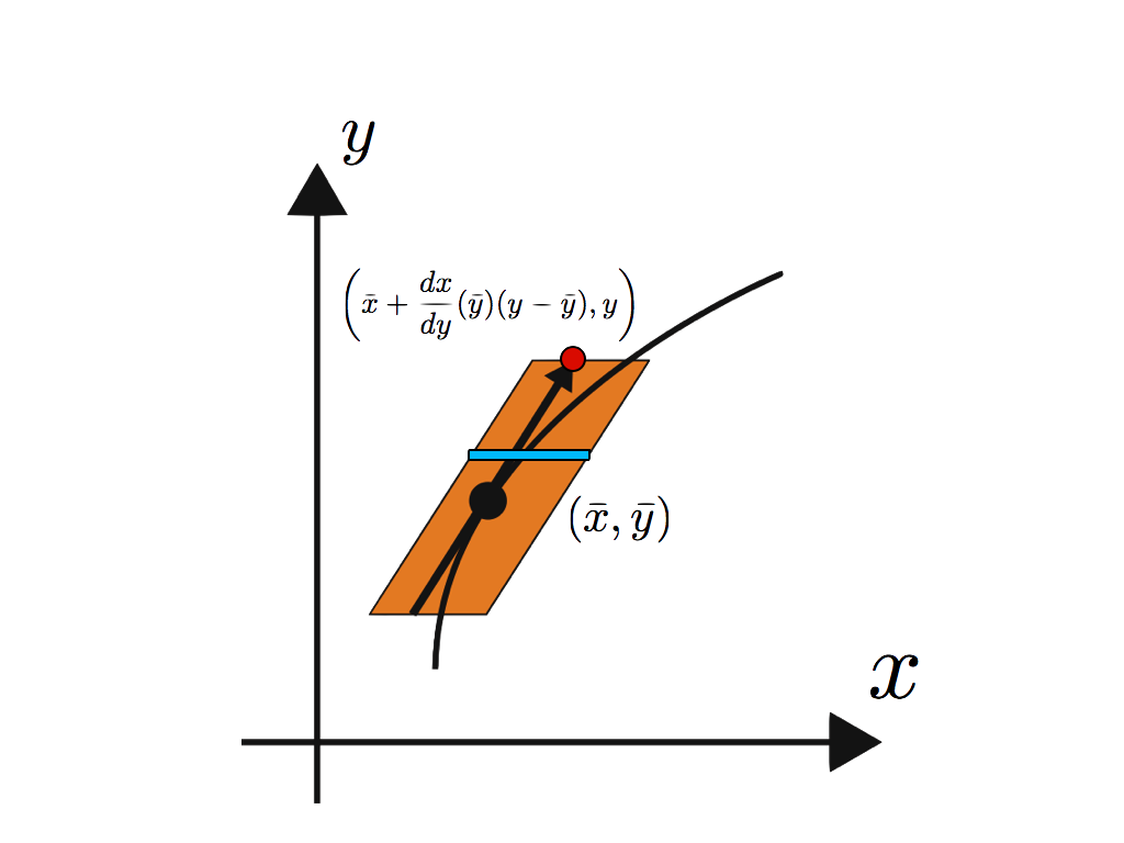
Here we provide another approach for validating fast-saddle-type blocks. In previous subsection, fast-saddle type blocks are constructed centered at , where is a small compact neighborhood of . All transformations concerning eigenpairs are done at a point . Fig. 1-(a) briefly shows this situation. On the other hand, we can reselect the center of the candidate of blocks so that blocks can be chosen smaller. As continuations of equilibria with respect to parameters, the predictor-corrector approach is one of effective approaches. We now revisit the construction of fast-saddle type blocks with the predictor-corrector approach.
Let be a (numerical) equilibrium for (1.3), i.e., , such that is invertible. Let be a compact neighborhood of . The central idea is to choose the center as follows instead of :
| (2.14) |
where is the parametrization of with respect to such that and that , which is actually realized in a small neighborhood of in since is invertible. See Fig. 1-(b). Obviously, the identification in (2.14) makes sense thanks to the Implicit Function Theorem.
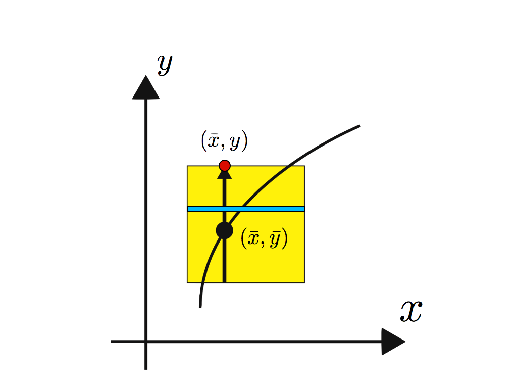
(a)
(b)
(a): The center point of blocks in -coordinate is fixed. The blue rectangle shows a fast-saddle-type block at . This procedure can be realized just by extending error bounds in (2.11) to -directions. However, the “higher order” term may contain the linear term with respect to . This may cause the increase of error bounds.
(b): The center point of blocks is moved along the tangent line (or plane for higher dimensional systems) at . The blue rectangle shows a fast-saddle-type block at . In principle, size of blocks will be smaller than (a) since the linear term with respect to in error term is approximately dropped.
Around the new center, we define the new affine transformation as
| (2.15) |
where is a nonsingular matrix diagonalizing . Over the new -coordinate, the fast system is transformed into the following:
where and , and . The function denotes the higher order term of with . Dividing into corresponding to eigenvalues with positive real parts and negative real parts, respectively, as in (2.10), we can construct a candidate set of fast-saddle-type blocks as in (2.12). By the similar implementations to Section 2.3.2, we can construct fast-saddle-type blocks centered at (2.14) for .
Note that the higher order term contains the linear term of as with small errors in a sufficiently small neighborhood of . This fact indicates that, in principle, size of blocks becomes smaller than those in Section 2.3.2, as seen in Fig. 1-(b). This benefit is also useful for the following arguments.
3 Slow manifold validations
In this section, we provide a verification theorem of slow manifolds as well as their stable and unstable manifolds. Our goal here is to provide sufficient conditions to validate not only the critical manifold but also the perturbed slow manifold of (1.1)ϵ for all in given regions.
Recall that Fenichel’s results (Propositions 2.2, 2.3) assume normal hyperbolicity and graph representation of the critical manifold . These assumptions are nontrivial, but very essential to prove the persistence. Our verification theorem contains verification of normal hyperbolicity and graph representation of .
The main idea is based on discussions in [18]. For technical reasons, we use a multiple of as the new auxiliary variable. We set and , where is a given positive number. We add the equation to (2.1). Furthermore, we consider the following system instead of (2.1) for simplicity:
| (3.1) |
Here denotes the matrix which all eigenvalues have positive real part and denotes the matrix which all eigenvalues have negative real part. Note that matrices and are (locally) independent of . This formulation is natural when we the construction of fast-saddle-type blocks stated in Section 2.3 is taken into account.
Let be a fast-saddle type block for (1.1). Section 2.3 implies that the coordinate representation, , is given by (2.12) (or (2.13)), which is directly obtained from the system (3.1). A fast-saddle-type block has the form (2.12), which has -coordinate, -coordinate and -coordinate following (3.1). With this in mind, we put following notations.
Notations 3.1.
Let , , , , and be the projection onto the -, -, -, -, - and -coordinate in , respectively. If no confusion arises, we drop the phrase “in ” in their notations.
We identify nonlinear terms , and with , and , respectively, via an affine transform .
For a squared matrix with , denotes a positive number such that
| (3.2) |
Similarly, for a squared matrix with , denotes a negative number such that
| (3.3) |
Finally, let be the distance between and , , given by .
The following assumptions are other keys of our verification theorem, so-called cone conditions.
Assumption 3.2.
Assumption 3.3.
Definition 3.4 (Cone conditions).
By following the proof of Theorem 4 in [18], we obtain the following theorem, which is the main result in this section.
Theorem 3.5.
Consider (3.1). Let be a fast-saddle-type block such that the coordinate representation is actually given by (2.12) with . Then
-
1.
if we assume
(3.8) there is an -dimensional normally hyperbolic invariant manifold in for the limit system (1.3) such that is the graph of a smooth function depending on .
-
2.
if the stable cone condition is satisfied, there exists a Lipschitz function defined in such that the graph
is locally invariant with respect to (3.1). Moreover, is for any on .
-
3.
if the unstable cone condition is satisfied, there exists a Lipschitz function defined in such that the graph
is locally invariant with respect to (3.1). Moreover, is for any on .
As a consequence, under stable and unstable cone conditions, can be defined by the locally invariant -dimensional submanifold of inside for any .
Proof.
Our proof is based on the slight modification of the proof of Theorem 4 in [18] for our current setting. The proof consists of three parts: (i) normal hyperbolicity and graph representation of , (ii) existence of the graph representation of and (iii) coincidence of the graph of such a derived function with all of . We shall prove them by tracing discussions in [18]. Readers who are not familiar with the invariant manifold theorem in singular perturbation problems very well can compare our discussions with Chapter 2 in [18]. Here we shall derive discussions only for the stable manifold , while discussions for the unstable manifold can be also derived replacing matrices in Assumption 3.3 by those in Assumption 3.2 and time reversal. Remark that an assumption for implies that all discussions are done in terms of (2.12). Without the loss of generality, we may assume .
- (i): Normal hyperbolicity and the graph representation of .
First of all, consider the special case . In this case, the slow variable is just a parameter. Inequalities in (3.8) yield the existence of local Lyapunov functions, which is a consequence of arguments in [23] with a little modifications as follows. Fix . Define a function by
where is an equilibrium for (3.1) with in at . The existence of follows from Proposition 2.17.
Then
Let be the -dimensional -vector and be the -zero matrix. Now we obtain
via the Mean Value Theorem, where . The same inequalities hold for . Similarly, we obtain
via the Mean Value Theorem, where . The same inequalities hold for . Summarizing these inequalities, we obtain
The right-hand side is strictly negative unless , which follows from (3.4) and (3.6). Obviously, if and only if . Therefore, is a Lyapunov function. This observation leads to the following facts:
-
•
is an equilibrium for (1.3) which is unique in with fixed .
-
•
The linearized matrix
is strictly negative definite for all . This implies that is a hyperbolic fixed point for the layer problem (1.3).
These observations hold for arbitrary . Thanks to the Implicit Function Theorem, we can construct the graph of a smooth -parameter family of such hyperbolic fixed points, which is . In particular, has the structure of normally hyperbolic invariant manifold with graph representation.
- (ii): The graph representation of .
We perform the modification to deal with slow directions. We choose a set whose interior contains so that its boundary is given by the condition for some function and that satisfies for all . The function is assumed to be normalized so that is a unit inward 111In the lecture note by Jones [18], denotes outward normal vector. We should remark that it is wrong. Indeed, we determine the immediate exit and entrance of a block later. Our claim here is that the exit is and does not contain . To this end, should be the inward normal vector. If we prove the existence of , is chosen as the outward normal vector. normal to . Let be a function that has the following values
We now modify our system (3.1) by adding the term , where is a positive number which remains to be chosen.
We add an equation for the small parameter . Following Jones [18], we use a multiple of as the new auxiliary variable, , and append the equation to (3.1), as noted in the beginning of this section. We then obtain the system 222This modification guarantees that the vector field has the inflowing property with respect to (e.g. [6, 10]). Namely, at any point , the vector field at goes inside . This property plays an important role to prove the existence of center-stable manifolds via the graph representation. In the case of or generally center-unstable manifolds, we modify the vector field so that the vector field has the overflowing property with respect to . Namely, at any point , the vector field at goes outside or tangent to . In our case, it is sufficient to choose the unit vector as the unit outward normal vector to and to choose in the similar manner to .
| (3.9) |
As in (3.1) it is understood that is a function of and , which is already realized in Section 2.3, and is a function of . If Theorem 3.5 is restated with replaced by and proved in that formulation, its original version can easily be recaptured by substituting back in.
We define the new family of sets by
Define the set
where is the flow generated by (3.9). In this part we shall prove that is the graph of a function of , say, . Set and denote the crossing section of at :
We shall show that there is at least one point for which for all . To achieve this, we use the Wazewski Principle. If the exit is closed in and is an isolating block for (3.9), then the mapping given by
is continuous. It is the general consequence of isolating blocks (see [31], Chapter 22. In [18], such is called Wazewski set). Since is of saddle-type, the flow is repelling on the fast-exit for all and is attracting on the fast-entrance for all . It is actually satisfied by choosing sufficiently small, if necessary. The rest are the -direction and the -direction. Note that an appropriate choice of enables us to construct local Lyapunov functions in (i) for all .
For points on with , we know
since holds on , where denotes an inner product on appropriate vector spaces. Setting , the above can be estimated by
if . Since we can choose arbitrarily, then it can be achieved. Therefore, is a part of entrance. Finally, in the case or , both of these sets are invariant since holds everywhere and thus render neither the entrance nor the exit.
The exit is then seen to be . By our construction of , for any , the set is a ball of dimension . Suppose that . All points in then go to in finite time and hence, restricting Wazewski map to the crossing section, we obtain a continuous mapping
If we follow this by the projection , we see that maps a -dimensional ball onto its boundary, while keeping the boundary fixed. This contradicts the well-known No-Retract Theorem. There is thus a point in . Since is arbitrary, this gives at least one value for as a function of . We shall put it .
- (iii): Uniqueness of as a graph of .
In the sequel we show that the graph of the above derived function is all of . At the same time, it will be shown that the function is, in fact, Lipschitz continuous with Lipschitz constant . A comparison between the growth rates in different directions will be derived in the following proposition in our setting. Let , , be two solutions of (3.9), set and . Further we define
Proposition 3.6 (cf. Lemma 2 in [18]).
Under assumptions of Theorem 3.5, if then holds as long as the two solutions stay in , unless .
Proof of Proposition 3.6.
Discussions in our proof are based on the proof of Lemma 2 in [18] with arrangements in our setting. We will make on each of the quantities etc. The equation for is
which we rewrite as
| (3.10) |
where . Since is the product of -sets associated with an affine transformation, thanks to the Mean Value Theorem, one can derive the following equality:
for some points . Such an estimate makes sense since is convex.
We can estimate by taking the inner product of (3.10) with . As a result, we obtain
| (3.11) |
We also obtain the following equalities in the same manner:
| (3.12) |
as well as
| (3.13) |
for some , . Obviously since .
Recall that our final objective is the estimate of . To this end, we estimate (3.11), (3.12) and (3.13) as the quadratic form associated with non-square matrices. For example, the equality (3.11) can be rewritten by the following matrix form:
where is the -matrix given by and is the -matrix given by
Denoting the (matrix) -norm, general theory of linear algebra yields
where , , is the maximal singular value of at stated in Assumption 3.3. We obtain the following estimate of (3.11):
| (3.14) |
where is a positive number satisfying (3.2). In the similar manner we also obtain the estimate of and by
where denotes a negative number satisfying (3.3). Functions , , and are maximal singular values of the matrix valued functions defined in Assumption 3.2 at , respectively.
In particular, at a point satisfying , we further obtain
to show
which proves our statement. Note that the coefficient of can be positive if is sufficiently small, thanks to cone conditions. ∎
We go back to the proof in (iii). We have already shown that the set contains the graph of a function denoted by . Suppose that contains more than one point with the same value of . There would then be and so that both and lie in . At , we have . By Proposition 3.6,
holds for all . In the estimate (3.14) we can then replace by to obtain
A positive number can be chosen as . See (3.4). From which it can be easily concluded that grows exponentially, which contradicts the hypothesis that both points stay in for all .
The same argument can be used to show that is also Lipschitz. If and are both in and , then grows exponentially, which contradicts the hypothesis again that both points lie in . We then have shown that the set is the graph of a Lipschitz function. In particular, the Lipschitz function is well-defined. This manifold is when is restricted to , in which the modified equation (3.9) agrees with the original one (3.1). Smoothness result follows from the same arguments as [18]. ∎
A direct consequence of graph representations of as well as is that they are homotopic to flat hyperplanes inside -sets. In terms of the theory of covering relations (Section 2.2), is a vertical disc and is a horizontal disc in a given fast-saddle-type block.
Corollary 3.7.
Proof.
Remark 3.8.
We do not need to assume the normal hyperbolicity of the critical manifold and the graph representation of in Theorem 3.5, while the Fenichel’s classical theory needs to assume them. Indeed, Part (i) in the proof of the theorem shows that this assumption can be validated by a computable estimate (3.8).
Remark 3.9.
It is well known that is not uniquely determined in general.
Let and be fast-saddle type blocks given by (2.12) and (2.13), respectively. Theorem 3.5 says that, under cone conditions, the slow manifold is contained in . Obviously is also contained in since . Moreover, is uniquely determined in . If , then our observations imply that the distance between and in fast components is greater than . For example, the distance of and in -component is greater than . Summarizing these arguments we have the following result, which is essential to Section 4.3.
Corollary 3.10 (Fast-saddle-type blocks with spaces).
Consider (2.10). Let be fast-saddle-type blocks for (2.10) such that the coordinate representations and are actually given by (2.12) and (2.13), respectively, for a given sequence of positive numbers . Assume that stable and unstable cone conditions hold in . Then the same statements as Theorem 3.5 holds in . Moreover, the distance between and the validated slow manifold is estimated by
The main feature of our present results is that slow manifolds as well as their stable and unstable manifolds in Fenichel’s theorems are validated in given blocks with an explicit range . Our criteria can be explicitly validated with rigorous numerics, as many preceding works (e.g. [35, 37]). We end this section noting that all results in this section holds if we replace and -valued function by and -valued function , respectively, with .
4 Covering-Exchange and dynamics around slow manifolds
In Section 3 we have discussed the validation of slow manifolds. In this section, we move to the next stage; the behavior near and on validated slow manifolds. There are mainly two cases of the exhibition of slow dynamics. One is monotone and the other is nontrivial in the sense that dynamics on slow manifolds admit nontrivial invariant sets such as fixed points or periodic orbits.
First we consider the dynamics near slow manifolds. If, for sufficiently small , a point is sufficiently close to slow manifolds, the trajectory through moves near slow manifolds spending a long time. However, the precise description of trajectories off slow manifolds is not easy since they clearly have an influence of fast dynamics . In order to describe such behavior as simple as possible, we introduce an extension of covering relations: the covering-exchange (Section 4.1), so that it can be appropriately applied to singular perturbation problems. This extension is a topological analogue of well-known Exchange Lemma. In the successive subsections, we provide a generalization of covering-exchange: the slow shadowing and -cones (Sections 4.2 - 4.4). These concepts enable us to validate slow manifolds with nonlinear structures as well as their stable and unstable manifolds in reasonable ways via rigorous numerics, keeping the essence of covering-exchange property.
Next, we consider the nontrivial dynamics on slow manifolds, namely, the presence of nontrivial invariant sets. We can use ideas discussed in Section 2.3 to validate nontrivial invariant sets even on slow manifolds.
Finally, we discuss the unstable manifold of invariant sets on slow manifolds. The invariant foliation structure with respect to slow manifolds is essentially applied to validating unstable manifolds of invariant sets in terms of covering relations.
4.1 Covering-Exchange with one-dimensional slow variable
First we consider the case that the vector field near slow manifolds is monotone. In such a case, geometric singular perturbation theory has an answer which describes dynamics around slow manifolds in terms of locally invariant manifolds; Exchange Lemma (e.g. [19, 20, 18, 33]).
Exchange Lemma solves matching problems between fast dynamics and slow dynamics. More precisely, if a family of tracking invariant manifolds have transversal intersection at , then a trajectory for a point describes the match of fast and slow trajectories near the slow manifold in the full system (1.1)ϵ for sufficiently small . However, Exchange Lemma requires the assumption of transversality between a tracking (locally invariant) manifold and the stable manifold of a slow manifold, which is not easy to validate in rigorous numerics. Alternatively, we consider the topological analogue of statements in (-)Exchange Lemma.
Every trajectories in fast-saddle-type blocks leaves them through exits. Note that our desiring trajectories are the continuation of chains consisting of critical manifolds and heteroclinic orbits in the limit system (1.3). One thus expects that singularly perturbed global trajectories leave fast-saddle-type blocks through fast-exits. To describe our expectations precisely, we define the following notions. For our purpose, we restrict for -sets to unless otherwise noted.
Definition 4.1 (Fast-exit face).
Let be an -dimensional -set with the following expression via a homeomorphism :
with and . We say an -set a fast-exit face of if , and there exist an element and a compact interval such that
See also Fig. 2.
Definition 4.2 (Covering-Exchange).
Consider (1.1)ϵ with fixed . Let be an -set with and be an -dimensional -set in with . We say satisfies the covering-exchange property for (1.1)ϵ with respect to if the following statements are satisfied:
- (CE1)
-
is a fast-saddle-type block with the coordinate system
- (CE2)
- (CE3)
-
For , holds in . We shall say the slow direction number.
- (CE4)
-
Letting be the flow of (1.1)ϵ, there exists such that .
- (CE5)
-
possesses a fast-exit face with the expression
such that
holds.
In this situation we shall call the pair the covering-exchange pair for (1.1)ϵ.
A brief illustration of the covering-exchange property is shown in Fig. 2. (CE2) implies the existence of the slow manifold as well as a limiting normally hyperbolic critical manifold at , as shown in Theorem 3.5. Combining with (CE1), one sees that is repelling in -direction and attracting in -direction. (CE3) means that slow dynamics in is monotone. Remark that the monotonicity is assumed not only on but also in the whole region . (CE4) topologically describes the transversality of the stable manifold of the slow manifold and the -set .
For a fast-saddle-type block of the form in Definition 4.2 with , we say and (equivalently and ) the slow exit and the slow entrance of , respectively. Similarly, in the case of , and be the slow exit and the slow entrance of , respectively.
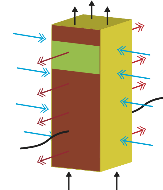
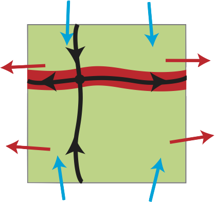
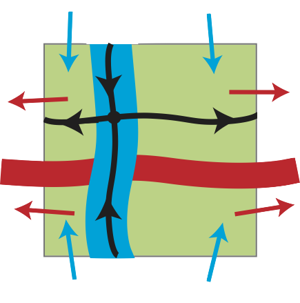
The rectangular parallelepiped is an -set with and . Arrows colored by red, blue and black show the fast unstable direction, fast stable direction and slow direction of (3.1) at corresponding boundaries, respectively. The black curve is an image of another -set for some . This figure describes . Since the -component of vector field in is monotone and the fast component of the vector field on is already validated concretely, then keeps the covering relation for all until exits from its top. A fast-exit face is colored by green, in which case .
Define the Poincaré map in by
If no confusion arises, we use this notation for representing the Poincaré map in a set .
Notations 4.3.
For and any set , let , and .
Lemma 4.4.
Fix . Let be a covering-exchange pair for (1.1)ϵ with the slow direction number and the fast-exit face with , where
Then, for each , the restriction of the Poincaré map to is a homeomorphism. Moreover, there exists an -set such that .
Proof.
Via a homeomorphism , we may assume that .
Since is an isolating block for , then is continuous on , which is the consequence of standard theory of isolating blocks [7, 18, 31]. Consider the backward Poincaré map given by
This is obviously well-defined via the property of flows. Since is also an isolating block for the backward flow, then the exit of in backward time is closed and hence is also continuous. The correspondence between points on and their image is one-to-one and onto under . This property holds since is a crossing section from (CE3). By restricting to and redefining and for , their continuity yields that is compact. Therefore, the restriction of to is a homeomorphism.
Next consider instead of . Since is a fast-saddle-type block with satisfying stable and unstable cone conditions, then the stable manifold divides into two components, where is the slow manifold in . Let be the component of containing . Now we can construct an -set with desiring covering relation as follows.
Consider a section . Let be such that . Since is homeomorphic, holds and
hold, Proposition 3.6 implies that with , , and satisfy . Here denotes the unstable cone with the vertex :
Thus there exist points such that with .
Let be given by . Thanks to the continuity of , both are continuous. Finally, define by
It is indeed an -set with
| (4.1) |
Slight modifications of yield the correspondence
We rewrite the corresponding -set as again.
Note that by definition of . Also, holds since is on . The arbitrary choice of leads to the statement in Proposition 2.8. In particular, holds. Of course, also holds since is just a restriction of in .
Moreover, the union also satisfies . Proof of the case is similar. ∎
The following proposition is the core of the covering-exchange property.
Proposition 4.5.
Let be a covering-exchange pair for (1.1)ϵ with a fast-exit face . Then there exists an -set such that
Proof.
Without the loss of generality, we may assume that and via a homomorphism , where . Also, let .
By Lemma 4.4, we can construct an -set depending on which -covers . Let be such an -set. Note that such an -set can be constructed for all . Now choose so that
and define a set by . The monotonicity of and homeomorphic correspondence of the flow imply that is actually an -set with , where are given by (4.1). The covering relation immediately holds from the proof of Lemma 4.4. Moreover, also holds by the construction of and the assumption . ∎
Proposition 4.5 shows that the covering-exchange property enables us to track solution orbits near slow manifolds. This is just a consequence of Proposition 2.11.
Remark 4.6.
Our implementations of covering-exchange property automatically solve the matching problem in singular perturbation problems. Indeed, let be a covering-exchange pair with a fast-exit face . In most cases, is a family of tracking invariant manifold whose behavior is mainly dominated by fast dynamics. On the other hand, the behavior of points in obtained in Proposition 4.5 is mainly dominated by the slow dynamics until it leaves . If such a point is also on , then we can prove the existence of a point which goes to along the fast dynamics in the first stage, stays dominated by the slow dynamics until it leaves through in the second stage and goes outside along the fast dynamics again in the third stage. The trajectory through is actually dominated by the full system (1.1)ϵ. Such a behavior is thus considered as the match of dynamics in different time scales.
One of other key points of the covering-exchange is that the choice of -dimensional variables is changed during time evolutions around slow manifolds. Indeed, the covering relation typically corresponds to validation of codimension connecting orbits between saddle-type equilibria in the limit system. In such a case, the -dimensional variable are chosen from -variables, while the -dimensional variables of are chosen from -variables: fast-unstable directions, which is natural from the viewpoint of codimension connecting orbits. Finally, during the covering relation , the -dimensional variables return to the part of -variables, since is regarded as the initial data of other codimension connecting orbits in the limit system. Consequently, we observe the “exchange” of the choice of -dimensional variables during the covering relation in Proposition 4.5. In this sense, we call this phenomenon the covering-“exchange”. Needless to say, one can describe such matching property without solving any differential equations in .
4.2 Expanding and contracting rate of disks
Assumptions of the covering-exchange in the previous subsection require that each branch of slow manifolds should be validated by one fast-saddle-type block. However, slow manifolds may have nontrivial curvature in general. It is not thus realistic to validate slow manifolds by one block with computer assistance without any knowledges of vector fields. To overcome such computational difficulties, we provide several techniques for generalizing conditions in the covering-exchange.
As a preliminary to next subsections, we consider the expansion and contraction rate of disks in a fast-saddle-type block. Consider the system (3.1). Note that in (3.1) is the -diagonal matrix such that all eigenvalues of have positive real part, and that in (3.1) is the -diagonal matrix such that all eigenvalues of have negative real part. Let be a fast-saddle-type block satisfying stable and unstable cone conditions for fixed . Without the loss of generality, via homomorphism , we may assume that
Here we also assume that holds in . Two cross sections then become the slow entrance and the slow exit of , respectively.
Definition 4.7.
An -Lipschitz unstable disk is the graph of a Lipschitz function with . Similarly, an -Lipschitz stable disk is the graph of a Lipschitz function with .
Next we consider the expanding and contracting rate of stable and unstable disks.
Lemma 4.8.
Let be a fast-saddle type block satisfying stable and unstable cone conditions. Let and be a -Lipschitz unstable disk and a stable disk of the diameter , respectively, contained in . Let be fixed.
- 1.
- 2.
The above inequalities imply that the expanding rate of is uniformly bounded below by and that the contracting rate of is uniformly bounded above by .
Proof.
1. Assume first that . The unstable cone condition with our assumption implies that and hold for all . In particular, holds for all . Let , and . The first variation equation in -direction yields
which is obtained by arguments in the proof of Proposition 3.6. Here we used the fact that holds in for all . This inequality leads to , and hence .
2. Next assume that . The stable cone condition with our assumption implies that and hold for all , where
In particular, holds for all .
The backward first variation equation in -direction yields
Here we used the fact that holds in for all . This inequality leads to , and hence . ∎
Note that Lemma 4.8 holds even when .
4.3 Slow shadowing, drop and jump
Under suitable assumptions, slow manifolds as well as limiting critical manifolds are represented by graphs of nonlinear functions. In such cases, it is not easy to validate slow manifolds by one block of fast-saddle-type. It is thus natural to construct enclosure of such manifolds by the finite sequence of fast-saddle-type blocks, which will be easier than validation by one -set. However, the union of finite fast-saddle-type blocks is not generally convex and hence we cannot apply arguments of the covering-exchange directly. In particular, we have to consider the effect of slow exits and slow entrances of the union. Nevertheless, the behavior in -direction is much slower than the behavior in -direction for sufficiently small . It is thus natural to consider that slow exits and entrances cause no effect on validation of trajectories sufficiently close to slow manifolds for (1.1). Here we construct a sufficient condition to explicitly guarantee such expectation. The key feature consists of two parts: (i) the comparison of expansion and contraction rate with the speed of slow vector field, and (ii) abstract construction of covering relations around slow manifolds. Our proposing concept named slow shadowing expresses both features. Slow shadowing can incorporate with the covering relations in Proposition 4.5; the drop corresponding to and the jump corresponding to . As a consequence, the concept of covering-exchange is generalized to the finite union of fast-saddle-type blocks.
The center of our considerations is a sequence of fast-saddle-type blocks satisfying all assumptions in Theorem 3.5. In this case, Theorem 3.5 indicates that the stable manifold is given by the graph of a Lipschitz function in each . Cone conditions also yield that these manifolds are patched globally in .
Lemma 4.9.
Let be a sequence of fast-saddle-type blocks satisfying all assumptions in Theorem 3.5. Assume that, for all , and that each section contains a unique point of the critical manifold . Then, for all , validated stable manifolds and in blocks and , respectively, coincide with each other in the intersection for . The similar result holds for .
Proof.
The same arguments as Theorem 3.5 for and with a fixed yield the result. ∎
Consider two fast-saddle-type blocks and . Assume that each is constructed in the local coordinate whose origin corresponds to such that (1.1) locally forms (3.1). Two coordinate systems are related to each other by the following commutative diagram:
| (4.2) |
where and be nonsingular matrices determining the approximate diagonal form (3.1) around and , respectively, and denotes the identity map on . The map denotes the composition map given by
We assume
- (SS1)
-
.
- (SS2)
-
. For given sequences of positive numbers , , is constructed by (2.13) with the sequence . The -component of is given by with
where is the projection onto the slow variable component.
- (SS3)
-
All assumptions in Theorem 3.5 are satisfied in and . Moreover, holds with the slow direction number in .
- (SS4)
- (SS5)
-
Fix positive numbers arbitrarily. Let and be families of disks given by
via and , respectively.
Then
(4.4) holds for all .
Since both and are linear maps, the covering relation (4.4) is just a transversality of rectangular domains relative to an affine map.
Definition 4.10 (Slow shadowing pair).
Let be a fixed number. Assume (SS1) - (SS5). We say the pair satisfies the slow shadowing condition (with the ratio and the slow direction number ) if the following inequality holds:
| (4.5) |
We shall say the pair the slow shadowing pair (with and the slow direction number ) if satisfies the slow shadowing condition (with ). We call the number the slow shadowing ratio.
In practical computations, we set sequences of positive numbers and , , as identical positive numbers, which make settings in practical computations simple. The assumption (SS5) admits a sufficient condition for validations in terms of cones. We revisit the condition in the end of Section 4.4.
The slow shadowing condition can be generalized to a sequence of fast-saddle-type blocks as follows.
Definition 4.11 (Slow shadowing sequence).
Consider a finite sequence of fast-saddle type blocks . We shall say the sequence of blocks and positive numbers satisfies the slow shadowing condition (with and ) if, for and satisfying (SS4), each pair is a slow shadowing pair with an identical slow direction number in Definition 4.10, where is the slow shadowing ratio for . We shall say such a sequence the slow shadowing sequence (with ).
The slow shadowing ratio gives us a benefit in practical computations. We mention this point concretely in Section 6.2.
The core of the slow shadowing is that all disks transversal to stable and unstable manifolds of slow manifolds rapidly expand and contract, respectively, so that covering relation on a crossing section can be derived. In what follows we only consider the case . The corresponding results to can be shown in the similar manner.
Proposition 4.12 (Slow shadowing).
Let be a slow shadowing pair with the ratio . Then there exist -sets with and such that
Proof.
For the simplicity, we assume . All arguments below are valid for general .
Let be the slow manifold validated in . For simplicity, we write , and .
First note that is an upper bound of the absolute speed in -direction. This implies that any point in which arrives at through the orbit in takes at least time . Also note that, and can be represented by families of -Lipschitz stable and unstable disks, respectively, which follows from cone conditions.
Let be the -neighborhood of in , namely,
Also, let be a section of at , namely,
Obviously, all points in is contained in the unstable cone , where is the unique point in . The local positive invariance of the unstable cone implies that , where is the solution orbit with and is the solution orbit with . This relationship holds for all until arrives at . Lemma 4.8-(1) then yields
The slow shadowing condition implies that the unstable disk expands through the flow, and all points on the boundary arrive at before the time if . In this case, has an intersection with for all . This observation holds for arbitrary .
The preimage thus satisfies
Note that is equal to .
Lemma 4.13.
The set is an -set.
Proof.
We may assume that via a homeomorphism . is contained in for some . For each , consider the section . Let be such that , which is uniquely determined for each . Note that, for each , is contained in . Since is homeomorphic, holds in and
then for all , there exists such that , which is uniquely determined by the property of flows. Notice that monotonically increases along the flow for all . Since is continuous, then depends continuously on and . As a result, we have a continuous graph given by . Then is given by
| (4.6) |
which is an -set. ∎
We go back to the proof of Proposition 4.12. The next interest is
Consider the behavior of sections in backward flow. Since each is a stable disk with Lipschitz constant less than , then each point is contained in , where is the unique point in . Lemma 4.8-(2) yields
The slow shadowing condition implies that the stable disk expands in -direction through the backward flow, and its boundary arrives at before the time if . Note that is an -set given by (4.6), which implies that there exists some such that the image must have intersections with for all . This observation holds for arbitrary with . Therefore, should be less than .
The same arguments enable us to construct an -set in the same way as under assumptions of (4.5). In this case, our assumptions and the definition of slow shadowing imply .
Boundaries of and are given by
where is the map associated with , which is constructed in the same way as .
Now we check if all assumptions in Proposition 2.8 hold with .
The estimate implies . Similarly, the estimate implies . From our constructions of and as well as Lemma 4.13, and can be regarded as families of horizontal and vertical disks in and , respectively. In particular, from (SS5), , where . This disjointness yields . Similarly, , which yields , where . The rest of assumptions obviously holds if we choose so that for some . The property of degree obviously holds since is just a composite of uniformly contracting and expanding maps in corresponding directions. ∎
Proposition 4.12 can be generalized to a slow shadowing sequence , which is straightforward.
The same arguments as Proposition 4.5 yield the following result: the covering-exchange : drop.
Proposition 4.14 (Covering-Exchange : Drop).
Let be a slow shadowing pair with the ratio . Assume that there is an -set such that holds for some , where . Then there are -sets and such that
Proof.
As in the proof of Proposition 4.12, we may assume .
Let and be as in Proposition 4.12 and . Obviously holds since . By the construction of , the covering relation also holds. ∎
We provide the slow shadowing when a fast-saddle type block admits a fast-exit face, which corresponds to the covering relation in Proposition 4.5: the covering-exchange : jump. We restrict the unstable dimension to in the current considerations.
Proposition 4.15 (Covering-Exchange : Jump).
Let be a slow shadowing pair with . Also, let be the fast-exit face of and . Assume that . Then there are -sets and such that
Proof.
As in the proof of Proposition 4.12, we may assume . The proof consists of two parts : (i) and (ii) . Part (i) is a consequence of Lemma 4.4 with additional property of . The assumption and slow shadowing condition allow to satisfy
Therefore, the same arguments as Proposition 4.12 yield , the statement (ii). Note that . See also Fig. 3-(e). ∎
(a)
(b)
(c)
(d)
(e)
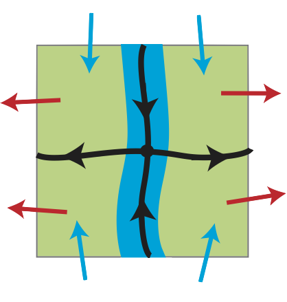
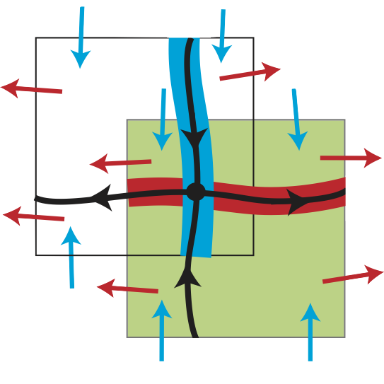
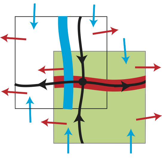
Note that all figures here show the projection onto the -space.
Slow shadowing : Covering relation in Proposition 4.12 is described by the process “(a)(b)(d)”, where is the Poincaré map in . A set colored by blue in (a) denotes . The Poincaré map maps to described by the red set in (b) and (d). The slow shadowing condition admits the choice of in drawn by the blue set in (d).
Covering-Exchange : Drop : Covering relation in Proposition 4.14 is described by the process “(c)(b)(d)”. In (c), the set colored by red denotes and the blue one denotes . The Poincaré map maps to described by the red set in (b) and (d). The slow shadowing condition admits the choice of in drawn by the blue set in (d).
Covering-Exchange : Jump : Covering relation in Proposition 4.15 is described by the process “(a)(b)(e)”. A set colored by blue in (a) denotes . The Poincaré map maps to described by the red set in (b) and (e). The slow shadowing condition admits the choice of in drawn by the blue set in (e). The -set -covers . The fast exit is drawn by the edge of white rectangle which admits horizontal red arrows.
For the convenience and correspondence to Definition 4.2, we introduce the following notion.
Definition 4.16 (Covering-exchange sequence).
Let be an -set and be a sequence of fast-saddle-type blocks. Assume that
- (Slow shadowing)
-
is a slow shadowing sequence with .
- (Drop)
-
holds for some , where is given in Proposition 4.14.
- (Jump)
-
is a slow shadowing pair with a fast-exit face of satisfying assumptions in Proposition 4.15.
Then we call the triple the covering-exchange sequence.
Obviously, the case is nothing but the notion of covering-exchange pair. Remark that, in the current setting, covering-exchange sequences are always assumed to be defined with .
Throughout the rest of this paper, the bold-style phrases Drop and Jump denote the corresponding descriptions stated in Definition 4.16.
4.4 -cones
We have discussed in Section 3 that it is systematically possible to construct fast-saddle-type blocks as well as cone conditions. However, such blocks are generally too small compared with validation enclosures of trajectories, if we try to validate covering-exchange sequences. Moreover, when we solve differential equations with a fast-exit face as initial data in this situation, solution orbits will hardly move in the early stage because the vector field is close to zero. This phenomenon causes accumulation of computation errors (e.g. wrapping effect) and extra computation costs (e.g. memory or time). In particular, there is little hope to validate covering-exchange sequences. Such difficulties can be avoided if we find a large fast-saddle type block directly. A direct approach would be finding crossing sections which form boundaries of a large fast-saddle type block. It is not realistic to find such sections via interval arithmetics because vector fields are nonlinear and we have to consider the effect of slow dynamics. In many cases, direct search of blocks would be based on trial and error, which is not systematic. Our aim in this subsection is to provide an appropriate method to overcome difficulties with respect to solving differential equations.
In Section 3, we have constructed cones of the form and with a vertex , where and . See Fig. 4-(a) for the illustration of cones and the unstable manifold of a saddle fixed point. One expects that, in a neighborhood of , for example, can be extended to like Fig. 4-(b).
On the other hand, if the unstable manifold is sufficiently regular, one also expects that such an extended cone can be sharper. More precisely, can be extended to the union of and a collection of -cones for some keeping isolation, which is shown in Fig. 4-(c). The same expectation is valid for .
Proposition 3.6 means that the difference of two solutions in a fast-saddle-type block along dynamics is restricted by the moving cone . The analogue of this argument in the case of sharper cones is derived below.
Assumption 4.17.
Consider (3.1). Let be an -set, and fix .
Proposition 4.18 (Unstable -cone).
Proof.
Do the same arguments as the proof of Proposition 3.6, replacing by . ∎
Assumption 4.19.
Consider (3.1). Let be an -set, and fix .
Proposition 4.20 (Stable -cone).
Proof.
Do the same arguments as the proof of Proposition 3.6, replacing by . ∎
Definition 4.21 (-cone conditions).
We shall call inequalities (4.7) and (4.8) in Assumption 4.17 the unstable -cone condition in . Similarly, we shall call inequalities (4.9) and (4.10) in Assumption 4.19 the stable -cone condition in . When these conditions are satisfied, the unstable -cone and the stable -cone with the vertex (in the -coordinate) are given as follows, respectively:
Validations of -cones themselves are in fact independent of the construction of fast-saddle-type blocks discussed in Section 2.3. Moreover, the choice of can be arbitrary as long as corresponding cone conditions hold.
An implementation of -cones in unstable direction is the following.
Lemma 4.22.
Let be a fast-saddle type block satisfying the stable cone condition, and be given by (4.11). Assume that the -unstable cone condition is satisfied in . Then any points on leaves the set
under the flow through . The sign is exactly the location of .
-cones in stable direction is constructed in the similar manner.
-
1.
Prepare a fast-saddle-type block such that is given by (2.13) satisfying the stable cone condition. Via a homeomorphism we may assume that is represented by
-
2.
Choose a face of the fast-entrance . As an example, set
where . Let is a given number and be an -set given by
(4.12) - 3.
The following lemma is a consequence of similar arguments to Lemma 4.22.
Lemma 4.23.
Let be a fast-saddle type block satisfying the stable cone condition, and be given by (4.12). Assume that the -stable cone condition is satisfied in . Then any points on leaves
under the backward flow through . The sign is exactly the location of .
Definition 4.24 (-cones).
We call the set of the form an unstable -cone of with the length . Similarly, we call the set of the form a stable -cone of with the length .
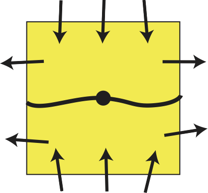
(a)
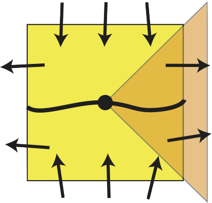
(b)
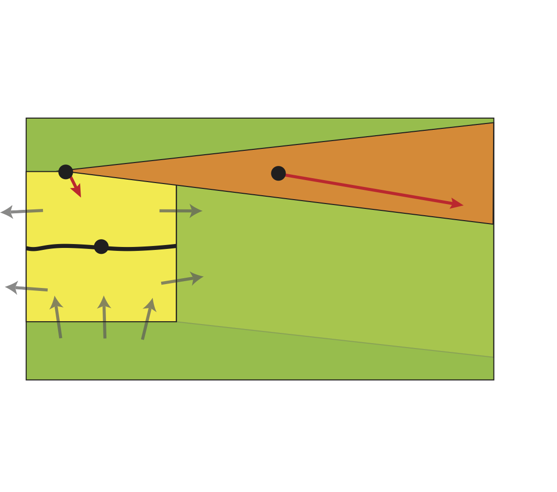
(c)
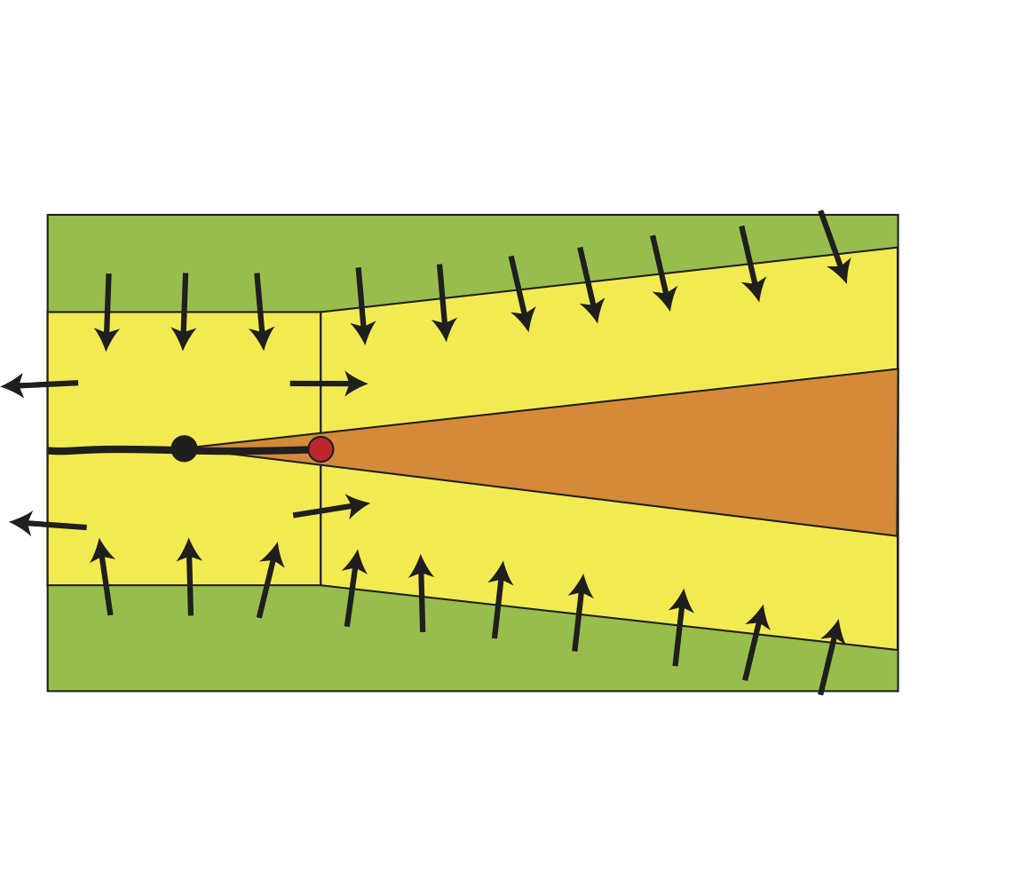
(d)
(a). A fast-saddle-type block containing the slow manifold validated in Theorem 3.5. In this figure, a black ball corresponds to slow manifold and a black curve corresponds to its unstable manifold . The accuracy of the stable (resp. unstable) manifold (resp. ) is measured by the size of the fast-entrance (resp. the fast-exit ). In general, blocks are small and the flow stay near those blocks for small , which cause the accumulation of various computational errors.
(b). A candidate of extended cones. One expect that our validated cones stated in Theorem 3.5. can be locally extended. However, one can imagine that it is quite too large for the enclosure of if is sufficiently smooth. The extension of cones drawn here is thus quite coarse for smooth manifolds.
(c). Validation of -cone condition. It is sufficient to verify -cone condition on a rectangular domain given by (4.11). The set is colored by green. The orange region is the -cone with a vertex in . -cone conditions imply that all points in an -cone stay the -cone until they leave .
(d). An unstable -cone of , which is the union of -cones with vertices on . The union is colored by yellow. All trajectories through leaves through . In general, is far from slow manifolds. This fact helps us with validations with reasonable computation steps and accuracy. See also Section 6.3.
Using -cones, we can extend an -set after construction of a small fast-saddle type block. Such an -set keeps isolation in radial direction, thanks to -cone conditions. Moreover, we can obtain a priori estimates of trajectories far from equilibria, keeping their accuracy as well as possible by adjustments of and . Of course, we do not need to solve differential equations to obtain such estimates. This technique reduces extra computation costs mentioned at the beginning of this subsection. Furthermore, in layer problems (1.3), -cones immediately yield continuation of stable and unstable manifolds of critical invariant manifolds. Indeed, the unions and are -sets satisfying -(un)stable cone conditions. The unstable (resp. stable) manifold is hence represented by a horizontal (resp. vertical) disk in (resp. ). See [39] for details.
Remark 4.25.
In what follows we show applications of -cones to fast-slow systems. In the case of fast-slow systems, we have to care about movements of trajectories in slow direction. With the help of slow shadowing condition, we can construct a sequence of covering relations for -cones. For technical reasons we restrict and to , in particular, . This is exactly the case in our verification examples, Section 6. Consider (3.1) again.
Definition 4.26 (Depature time, Arrival time).
Let be a fast-saddle-type block such is given by (2.13) with . Also, let be a set of the form (4.11) with satisfying the unstable -cone condition. Define the departure time in by
| (4.13) |
where is a given number in (SS5), , is given in (4.3), is a sufficiently small number,
and is a real number satisfying (3.2). Note that the unstable -cone condition implies that for .
Similarly, let be a set of the form (4.12) with satisfying the stable -cone condition. Define the arrival time in by
| (4.14) |
where is a given number in (SS5), , is given in (4.3), is a sufficiently small number,
and is a real number satisfying (3.3). Note that the stable -cone condition implies that for .
Remark 4.27.
The following results show that -cones generate additional covering relations to validate global orbits for (1.1)ϵ.
Proposition 4.28.
Let be a fast-saddle-type block for (3.1) in with which forms
and actually given by (2.13). Also, let be a set of the form (4.11) with which contains . Assume that the unstable -cone condition is satisfied in . Let be the departure time in . Define
| (4.15) |
where is chosen so that either or holds. Then holds.
Proof.
Let and be such that and that . The unstable -cone condition and Lemma 4.18 imply that for all until arrives at , where is given in Lemma 4.22. The difference satisfies
which follows from the same argument as the proof of Lemma 4.8. This implies that the solution orbit with arrives at at time and that
Thus holds. Note that consists of
Moreover, holds by Proposition 4.18. Then holds by Proposition 2.8 with . ∎
Definition 4.29.
We shall call given in (4.15) the fast-exit face of .
The following statements also hold from the same arguments under the backward flow.
Proposition 4.30.
Let and be fast-saddle-type blocks for (3.1) in with which form
such that is a slow shadowing pair with the slow direction number and given below. Also, let be a set of the form (4.12) with containing . Assume that the stable -cone condition is satisfied in . Let be the arrival time in . Define
Assume that there is an -set and such that and that
| (4.16) |
Let be such that .
Then there exist -sets and such that
Proof.
First let is the slow manifold validated in . Also, let and be -sets such that , which are constructed in Proposition 4.12. Note that contains . Let and . Clearly the set contains .
Next, let and be such that . The stable -cone condition and Lemma 4.23 imply that for all until arrives at under the backward flow. The difference satisfies
by the same argument as the proof of Lemma 4.8, where . This inequality implies that the backward solution orbit with arrives at at time and that
Define an -set , where
Note that follows from (4.16) and . The relationship immediately follows from . Then the covering relation also follows from .
∎
Slow shadowing sequence with extended -cones determine the generalized sequence of covering-exchange sequence in Definition 4.16.
Definition 4.31 (Covering-exchange sequence with extended cones).
Consider (1.1)ϵ in . Let be an -set with and be a sequence such that
Another benefit of -cones is that we can validate the assumption (SS5) in slow shadowing in terms of -cones. In the following proposition, we do not any restrictions on and .
Proposition 4.32 (A sufficient condition of (SS5)).
Consider two fast-saddle-type blocks and constructed in the local coordinate , where (1.1) locally forms (3.1) in each coordinate with the commutative diagram (4.2). Assume that both and satisfy the unstable -cone condition and the stable -cone condition for , and that (SS1)-(SS4) are satisfied.
Independently, consider two -sets and given by
via and , respectively, where denote positive numbers given in (SS4)-(SS5). Write the nonsingular matrix in (4.2) into the block form
where the first row acts on the -dimensional vector and the second row acts on the -dimensional vector . Finally assume that
and that
| (4.17) |
where and are the maximal and the minimal eigenvalue of the matrix , respectively, and denotes the maximal singular value of . Then (4.4) holds.
Proof.
First we set
corresponding to the -set structure.
We embed and on and , respectively, so that the origin of both and is the point . We write the embedded sets as and again, respectively. Without the loss of generality, we may assume that the representation of in -coordinate is given by . Note that, in this case, is a family of horizontal disks in and is a family of vertical disks in .
Define two sets and as follows. See also Fig. 5:
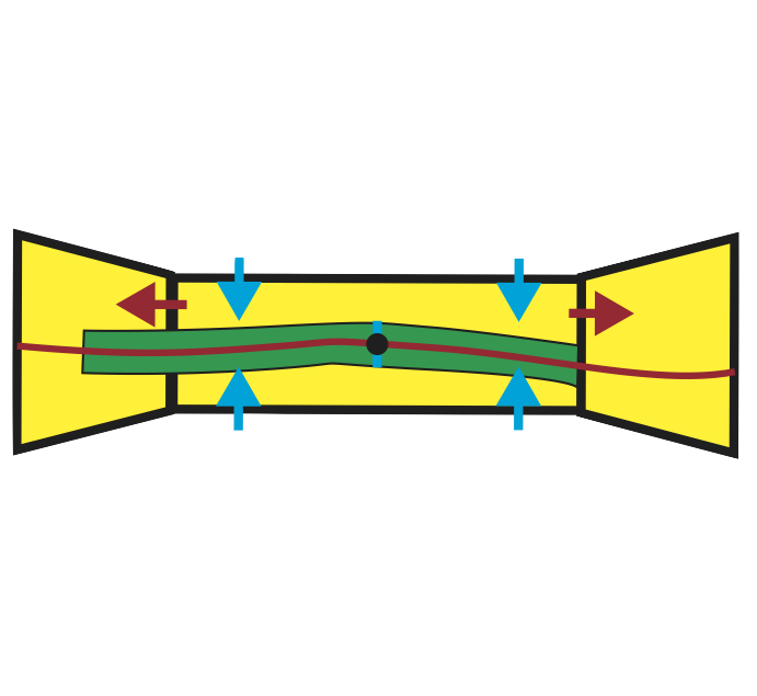
(a)
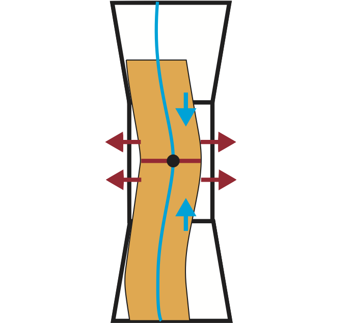
(b)
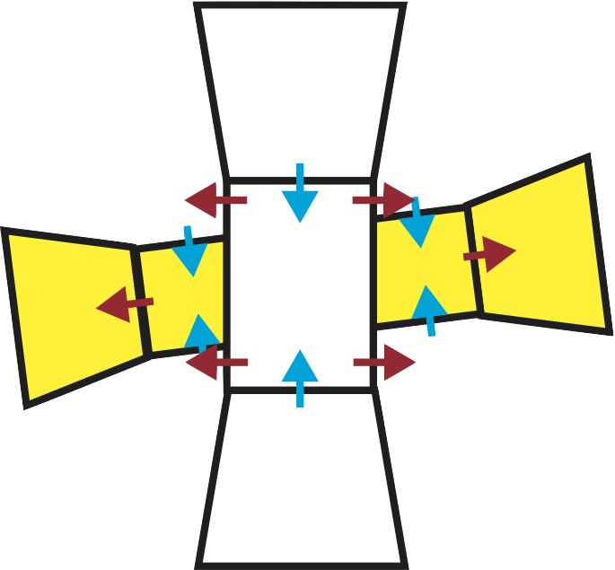
(c)
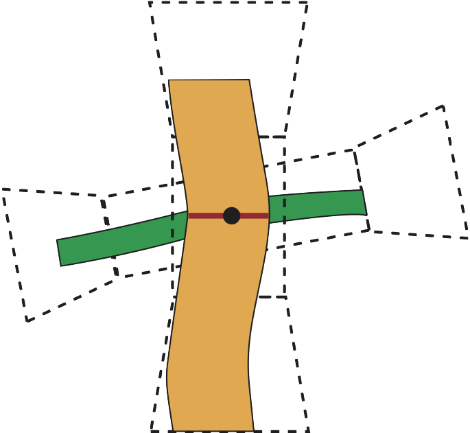
(d)
(a) : The set with , where . The red curve represents the slice of the unstable manifold by . The green tube represents the set . Definition of and the unstable -cone conditions indicate the inclusion . Note that consists of a collection of horizontal disks.
(b) : The set with , where . The blue curve represents the slice of the stable manifold by . The orange tube represents the set . Definition of and the stable -cone conditions indicate the inclusion . Note that consists of a collection of vertical disks.
(c) : Covering relation and (4.17). The inequality (4.17) indicates that two cones outside and are sufficiently sharp satisfying .
(d) : Resulting covering relation (4.4).
The unstable -cone and the stable -cone conditions imply that and , where and are given in (SS5) and . Indeed, is given by a tube in . The unstable manifold is contained in the unstable -cone . If runs on the range in -direction, the enclosure of in -direction is bounded by . The similar arguments yield that the enclosure of the tube in -direction is bounded by . Relations between unstable manifolds through and thus yield that . The similar arguments to yield the second. In particular, the covering relation implies (SS5). Note that this argument is independent of , in particular, .
By the construction of and , it is sufficient to prove the following two conditions to verify :
-
•
.
-
•
.
The former is just one of our assumptions. The latter concerns with intersections between subsets of cones. Since an -cone is a collection of lines inside through , it is sufficient to consider the location of lines through base sets.
Now we consider the image of the unstable -cone under . Since is the nonsingular affine map, any lines are mapped into lines via .
Choose a point . The boundary is a subset of . The transformation yields
The triangular inequality yields
Thus
further,
equivalently,
Let
The above inequality indicates that any line in is mapped into another one included in for some . By our construction, we know that any (half) lines in lie on ones with vertices in . Such vertices can be also chosen as points on , which are disjoint from . Remark that follows from the covering relation .
For any point , we easily know that if . This implies that any lines in are disjoint from with . This fact holds for any .
On the other hand, for any point , there is a point such that , which follows from the property of cones and the structure of from the covering relation . Consequently, we know that the set is contained in the union of with .
Combining these observations, we obtain . ∎
4.5 Invariant sets on slow manifolds
Next we consider invariant sets on slow manifolds. When , the dynamics on slow manifolds can generally exhibit non-trivial dynamics. In other words, slow manifolds can have nontrivial invariant sets, such as equilibria, periodic orbits and so on, for slow dynamics. Such sets play a key role for describing nontrivial global solutions such as singularly perturbed homoclinic or heteroclinic orbits.
Consider the slow manifold in a fast-saddle type block with stable and unstable cone conditions. Theorem 3.5 implies that is represented by the graph of a function smoothly depending on and including . Substituting into (1.1), one sees that the -equation will decouple from the -equation. Since is parameterized by , the resulting decoupled equation
describes the dynamics on . After time rescaling we obtain
| (4.18) |
to show that the dynamics on slow manifolds is reduced to the regular perturbation problem. Taking the limit in (4.18) we obtain the dynamics on the critical manifold :
| (4.19) |
When we want to study dynamics on slow manifolds, such as the existence of fixed points and their stability, (4.18) as well as (4.19) are in the center of our considerations.
In general, what we know about is just the fact that it is the graph of a function , and its concrete description is quite difficult to obtain. As for the normally hyperbolic critical manifold , we know that it is the subset of the nullcline . From such a fact, we can study the detail of such as the differential of as a -function via implicit function differential equation . On the contrary, the function does not possess such simple and useful properties. For example, does not necessarily hold. In general, is the solution of the following nonlinear partial differential equation:
| (4.20) |
In order to calculate the differential for studying the stability of fixed points on slow manifolds, for example, we have to solve the equation (4.20) rigorously. Nevertheless, from the viewpoint of rigorous numerics, it will be more reasonable regarding as with small errors (in -sense) than solving (4.20) directly. With this in mind, we consider (4.18) as the differential inclusion
where is a fast-saddle type block containing . The right-hand side possesses as the representative of the enclosure.
As an example of dynamics on via rigorous numerics, we consider the validation of fixed points for (4.18) on as well as their stability for . Thanks to regular perturbation relationship between (4.18) and (4.19), it is natural to consider that the fixed point of (4.18) on will be close to that of (4.19) on . We then rewrite (4.18) as
Using the Mean Value Theorem, the error term possesses the following expression:
The difference between and can be estimated by . Here corresponds to the size of the -th component in -coordinate of a fast-saddle-type block obtained by rigorous numerics. It is precisely computable. Such an estimate can be done because both and belong to an identical -set. Finally we obtain the following estimate:
| (4.21) |
Let be the numerical zero of . The principal part can be then expanded by
The Jacobian matrix at can be explicitly calculated via the Implicit Function Theorem to obtain
One can explicitly calculate eigenvalues of , which will be close to those of the Jacobian matrix of for . On the other hand, the chain rule yields
and it contains arisen in (4.20). We additionally need to the Fréchet differential of error terms of the form , when we try to validate the unique existence or hyperbolicity of equilibria via cone conditions [39] or Lyapunov conditions [23], for example. Instead, we apply a topological tool with to validation of invariant sets on slow manifolds.
Here we construct an isolating block on slow manifolds. Using enclosures like (4.21) and eigenvalues of , we can compute the rigorous enclosure of vector fields on crossing sections on slow manifolds.
Consider the case , which is our original setting. Assume that we have an -parameter family of slow manifolds as well as the critical manifold , which can be validated by the method in Section 3. Then one would have obtained a fast-saddle-type block surrounding . The schematic illustration of such a procedure is shown in Fig. 6. Let be a numerical zero of . One expects that there exists an equilibrium on for sufficiently small . We calculate the enclosure of on for small in such a situation. It can be done by
where can be determined by the size of . Remark that the enclosure of all terms in the right-hand side are rigorously computable and that they make sense for all . The principal term is . is very close to since is assumed to be the numerical zero of . If
| (4.22) |
are validated on , then the set is an isolating block on for with the attracting boundary. Similarly, if
| (4.23) |
are validated on , then the set is an isolating block on for with the repelling boundary. In both cases, the general Conley index theory [7] yields that for all . is actually the -parameter family of invariant sets on slow manifolds. The direction of vector fields corresponds to the stability of . Moreover, Proposition 2.17 shows the existence of an equilibria in for (4.18), which leads to an equilibrium in the full system (1.1). Note that isolating blocks can be constructed by the same implementations as Section 2.3.
Remark 4.33.
In terms of the Conley index theory, constructed sets are singular isolating neighborhoods. Indeed, for , consists of the curve of hyperbolic equilibria and hence it is not an isolating neighborhood. On the other hand, for it is an isolating neighborhood for .
Remark 4.34.
All validation of vector fields such as (4.22) and (4.23) make sense only on slow manifolds , since the decoupled vector field (4.18) makes sense only on slow manifolds. In other words, estimates of vector fields discussed here does not always give reasonable information of vector fields off slow manifolds. Calculations of vector fields discussed here and Section 4.1 should be thus considered independently.
A simpler way to study the dynamics on slow manifolds will be to focus on the dynamics (4.19), namely, neglect the error term . We then study the dynamics (4.18) on slow manifolds via the regular perturbation theory. The essence of this idea is the same as ours, but such results make sense only for sufficiently small . One of our main purpose here is to study the slow dynamics for all and hence such a simpler idea is not sufficient to our study.
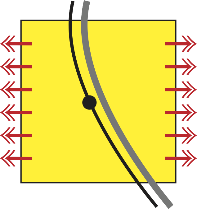
(a)
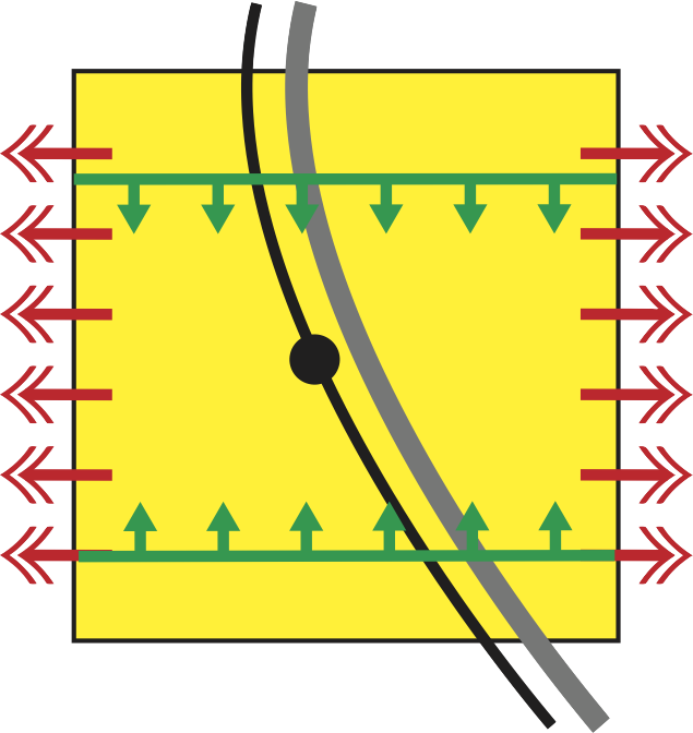
(b)
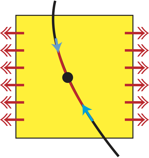
(c)
(a). Critical manifold (, colored by ash), and perturbed slow manifold (, colored by black) via Theorem 3.5. The yellow rectangle with red arrows describes a fast-saddle-type block with the fast-exit. The critical manifold is a subset of nullcline . In general, exhibits a nontrivial structure such as equilibria (drawn by a black ball).
(b). Validation of vector fields on . One cannot detect the position of the slow manifold in advance. In order to detect vector field on such invariant manifolds, one put a section (colored green) having an intersection with and validate the vector field on via rigorous numerics. This contains information of the vector field on .
(c). An illustration of isolating block containing an equilibrium on . Analysis in (b) contains the information of rigorous vector field on , which gives an isolating neighborhood colored by red. General topological arguments such as the mapping degree or the Conley index guarantee the existence of nontrivial invariant sets. In the case of illustration described here, there exists a fixed point on , namely, an equilibrium of the full system (1.1).
4.6 Unstable manifolds of invariant sets on slow manifolds
We discuss the unstable manifold of invariant sets in the full system. Combining covering-exchange property with graph representations of locally invariant manifolds, the standard consequence of covering relations, Proposition 2.14, yields the existence of connecting orbits between slow manifolds for (1.1)ϵ. However, it does not always mean the existence of connecting orbits between invariant sets for (1.1)ϵ. This difference comes from the fact that the meaning of slow variable changes between and . When we apply covering relations to connecting orbits between equilibria for (1.1)0, namely (1.3), a natural approach is to prove the existence of orbits connecting points on the stable and unstable manifolds of equilibria at a certain . This immediately yields validation of a connecting orbit at . On the other hand, if , a parameter becomes a time dependent variable and slow manifolds do not always consist of a family of equilibria or general invariant sets. In fact, if unstable manifolds of normally hyperbolic invariant manifolds are perturbed for , then the negatively invariant manifolds (e.g. unstable manifolds) of invariant sets are drastically collapsed in general. In particular, dimensions of -sets corresponding to unstable manifolds of invariant sets change. The standard arguments of covering relation is not thus sufficient to validate connecting orbits in (1.1)ϵ.
To overcome this difficulty, we apply further structure of slow manifolds, called Fenichel fibering, to validate (un)stable manifolds of invariant sets on slow manifolds.
A direct consequence of discussions in the previous subsection is stated as follows. This result can be generalized in arbitrary dimensions, but we omit the detail because we do not make such generalized arguments in this paper.
Lemma 4.35.
Let be a fast-saddle type block for (1.1)ϵ satisfying stable and unstable cone conditions, and be a subset of -dimensional slow manifold in . Assume that is an isolating block on the slow manifold whose boundaries are repelling (cf. (4.23)). Then a trivial collection is admissible with respect to for all sufficiently small (cf. Definition 2.12).
Similarly, assume that is an isolating block on the slow manifold whose boundaries are attracting (cf. (4.22)). Then a trivial collection is back-admissible with respect to for all sufficiently small .
Here we regard the flow in the full system as restricted to in both cases. This restriction makes sense since slow manifolds are locally invariant.
Since is -dimensional, if is repelling, the covering relation is nothing but . Similarly, if is attracting, the back-covering relation is nothing but . For simplicity, we write -covering relations for an -set and a continuous map by . Let be defined by the similar manner.
Lemma 4.35 gives the other proof of existence of an invariant set in . Note that this invariant set is actually invariant for the full system (1.1)ϵ.
A key essence of Fenichel fibering is cone conditions, which is the same as invariant manifold theorem. On the other hand, our statements in Theorem 3.5 involve cone condition which are computable via rigorous numerics. Theorem 3.5 thus yields the following fiber validations.
Corollary 4.36.
Consider (3.1). Let be a fast-saddle-type block such that the coordinate representation is actually given by (2.12) with . Assume that stable and unstable cone conditions are satisfied in and let be the validated slow manifold. Then for each , the following statements hold.
-
1.
There exists a Lipschitz function defined in a neighborhood of in and such that the graph
is locally invariant with respect to (3.1).
-
2.
There exists a Lipschitz function defined in a neighborhood of in and such that the graph
is locally invariant with respect to (3.1).
These functions are well-defined in a neighborhood of each , which means that, for example, may have an intersection with . In other words, is not always a horizontal disk in in the sense of Definition 2.13.
In the case of fast-slow systems, the property that becomes a horizontal disk in is nontrivial, which is due to dynamics in slow direction.
From now on we relate the fiber bundle structure of slow manifolds to covering relations. Fiber bundle structure of for leads to construct a deformation retract of unstable manifolds so that the fiber bundle -covers a fast-exit face. Namely, the following lemma holds.
Lemma 4.37.
Consider (3.1). Let be a fast-saddle-type block with such that the coordinate representation is actually given by . Also, let be a fast-exit face of with
and be a connected subset of -dimensional slow manifold in .
Assume that, for any , the Lipschitz function is a horizontal disk in . We also assume that, at with , and hold.
Then , where is the deformation retract given by
| (4.24) |
If , then the same statement holds by replacing in (4.24) by
| (4.25) |
Proof.
If we additionally assume that is a singular isolating neighborhood, then we can describe unstable manifolds of invariant sets.
Proposition 4.38.
In addition to assumptions in Lemma 4.37, we assume that is an isolating block on the slow manifold. Then there exists a point such that .
Proof.
Since is isolated, Lemma 4.35 yields the covering relation for arbitrary and all sufficiently small if is repelling. Similarly, if is attracting, the covering relation holds for arbitrary .
We only deal with the attracting case. By Proposition 2.11 there exists a point such that
| (4.26) |
Since is compact, then the sequence contains a convergence subsequence. Let be the limit. We can choose a sufficiently small such that holds for all , since is an isolating block. Note that means the boundary with respect to the slow manifold in . Obviously we can choose a limit point from (4.26) with . The property of and (4.26) thus imply for all , which yields . The inclusion is obvious since is attracting. As a consequence, . By continuity of the graph with respect to , then is well-defined and . ∎
The validation of being an isolating block on slow manifolds can be done by arguments in Section 4.5. On the other hand, if we apply Lemma 4.37, we have to know the location of fibers for all . The unstable (-)cone condition indicates that, for , the fiber is included in the unstable cone . We can apply this cone to validate assumptions in Lemma 4.37. Namely, the following lemma holds, which can be validated by rigorous numerics.
Lemma 4.39.
Consider (3.1). Let be a fast-saddle-type block with such that the coordinate representation is actually given by . Also, let be a fast-exit face of with
and be a connected subset of -dimensional slow manifold in . Assume that, for some , the unstable -cone condition is satisfied in and that, at , the unstable -cones satisfy the following properties:
| (4.27) | ||||
| (4.28) |
Then all assumptions in Lemma 4.37 hold.
Proof.
5 Topological existence theorems of singularly perturbed trajectories
Now we are ready to state our verification theorems. In this section we derive existence theorems for periodic and heteroclinic orbits which can be applied to (1.1).
5.1 Existence of periodic orbits
First we state the existence theorems for periodic orbits near singular orbits.
Theorem 5.1 (Existence of periodic orbits.).
Consider (1.1). Assume that there exist , such that (1.1) admits the following -parameter family of sets in (see also Fig. 7-(a)):
- :
-
: a fast-saddle-type block satisfying the covering-exchange property with respect to defined below and for .
- :
-
: a fast-exit face of . Identify with .
Then the following statements hold.
- 1.
-
2.
When , (1.1) admits the collection of heteroclinic orbits with
bridging -dimensional normally hyperbolic invariant manifolds and for . In case that such a heteroclinic orbit connects and .
Proof.
First consider the case . By Proposition 4.5 and our assumption, there exist -sets such that we get the sequence of covering relations
where is the Poincaré map of . Then our statement is just the consequence of Proposition 2.11. The case is just the consequence of Proposition 2.14. All arguments with respect to horizontal and vertical disks are valid from Corollary 3.7. ∎
Remark 5.2.
Standard Exchange Lemma says that the period when trajectories stays near slow manifolds in -distance is (actually for some , discussed in [19]). The period is thus expected to be for .
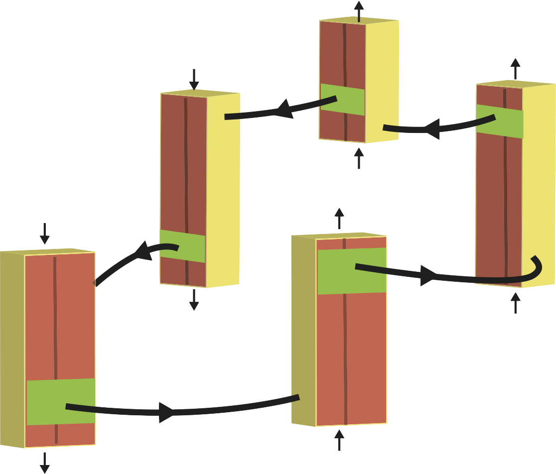
(a)
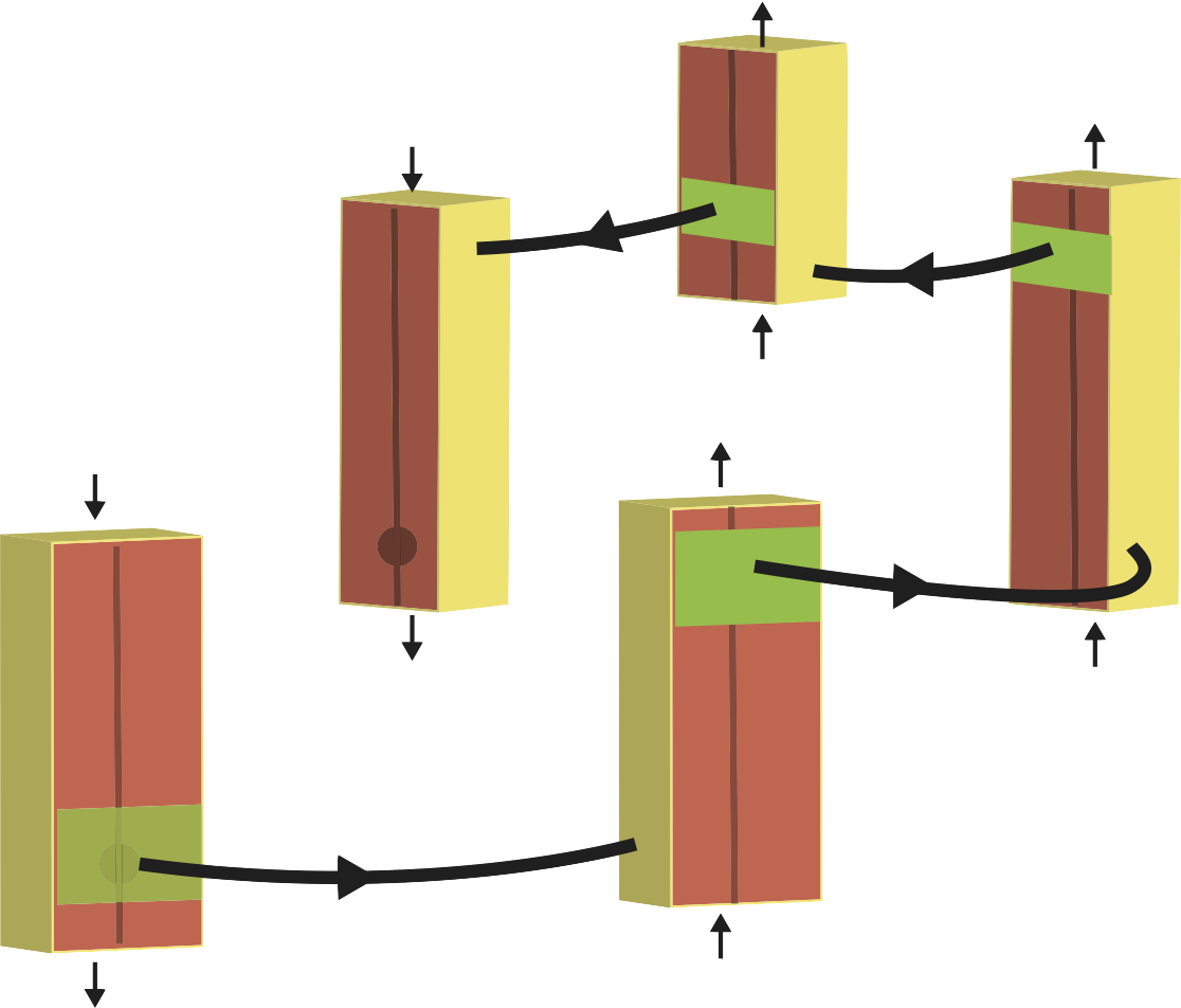
(b)
Rectangular parallelepipeds (colored red and yellow) are fast-saddle-type blocks with fast-exit faces (colored by green) satisfying the covering-exchange property. Vertical black arrows show the slow vector field. Bold black curves outside blocks describe heteroclinic orbits . Black lines inside blocks correspond to limit critical manifolds. Their union generates a singular limit orbit . Theorem 5.1 claims that there exists a family of periodic orbits near .
Theorem 5.1 can be generalized as stated below, replacing covering-exchange pairs by covering-exchange sequences.
Corollary 5.3 (Validation of periodic orbits with slow shadowing).
Proof.
We only consider the case . By Propositions 4.12, 4.14, 4.15 and our assumptions, there is a sequence of -sets with which admits a sequence of covering relations
where is the Poincaré map in with appropriate choices of and following Propositions 4.12, 4.14 and 4.15. Then our statement is just the consequence of Proposition 2.11. ∎
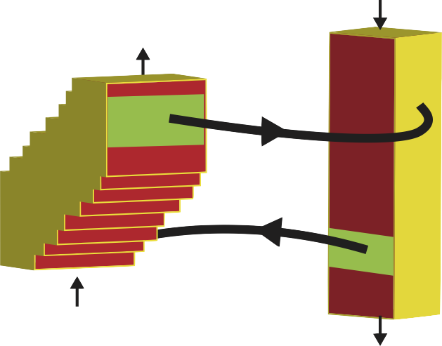
Rectangular parallelepipeds (colored red and yellow) are fast-saddle-type blocks with fast-exit faces (colored by green) satisfying the covering-exchange property and slow shadowing. Vertical black arrows show the slow vector field. Bold black curves outside blocks describe heteroclinic orbits and curves or surfaces inside blocks correspond to limit critical manifolds. Their union generates a singular limit orbit . Theorem 5.1 claims that there exists a family of periodic orbits near .
Note that points on the slow manifold are contained in all -sets in the proof of Corollary 5.3. This observation implies that true orbits in the full system (1.1) shadow trajectories on via covering relations (cf. [26]). This fact gives us a suggestion to describe true trajectories for fast-slow systems with multi-dimensional slow variables from the viewpoint of shadowing.
Corollary 5.3 can be further generalized as stated below, at least in the case , replacing covering-exchange sequences by covering-exchange sequences with extended cones.
Corollary 5.4 (Validation of periodic orbits with slow shadowing and -cones).
Consider (1.1). Assume that there exist , such that (1.1) admits the following -parameter family of sets in (see also Fig. 7):
- :
-
a sequence of fast-saddle type blocks which admits a sequence of faxt-exit faces with .
The collection forms a covering-exchange sequence with extended cones . Associating sets , and are defined below.
- :
-
the unstable -cones of . Identify with .
- :
-
the stable -cone of .
- :
-
a fast-exit face of . Identify with .
Then all statements in Theorem 5.1 hold with .
Proof.
Remark 5.5.
The key essence of our validation near slow manifolds consists of the following three pieces:
-
•
Construction of fast-saddle-type blocks;
-
•
Stable and unstable cone conditions;
-
•
Slow shadowing condition (if necessary).
As long as validations of the above procedures pass, we can extend slow manifolds in an arbitrary range keeping the existence of points near slow manifolds which exits their neighborhoods after time , as stated in the Exchange Lemma.
5.2 Existence of connecting orbits
Similar settings and arguments to the previous subsection yield the existence of heteroclinic orbits near singular orbits.
Theorem 5.6 (Existence of heteroclinic orbits).
Consider (1.1). Assume that there exist and such that (1.1) admits the following -parameter family of sets in (see also Fig. 7-(b)):
- :
-
: a fast-saddle-type block satisfying stable and unstable cone conditions. Moreover, it contains the nonempty maximal invariant sets .
: a fast-saddle-type block satisfying the covering-exchange property with respect to (defined below) except condition 3. Moreover, it contains the nonempty maximal invariant set . The set is contained in an attracting isolating block on the slow manifold in .: a fast-saddle-type block satisfying the covering-exchange property with respect to defined below and for .
- :
-
: a fast-exit face of .
If , the invariant set admits an isolating block on the slow manifold in such that all assumptions in Lemma 4.39 holds.
Proof.
Consider the case . We deal with the case that is attracting. By Propositions 4.5, 4.38 and our assumption we get the sequence of covering relations
for all sufficiently small and arbitrary . Here is the deformation retract given by (4.24) or (4.25), is the horizontal disk at whose graph is the unstable manifold and is the Poincaré map of . The stable manifold is given by a vertical disk in with -coordinates as the -dimensional direction of the -set . Our statement is just the consequence of Propositions 4.38 and 2.14. See Definition 2.13 about horizontal and vertical disks. All arguments with respect to horizontal and vertical disks are valid from Corollaries 3.7 and 4.36. In the case that is repelling, the same arguments valid replacing the covering relation by .
The case is the same as that of Theorem 5.1. Remark that we do not need the sequence of covering relations
to prove our statements in this case. ∎
Theorem 5.6 can be generalized as stated below, replacing covering-exchange pairs by covering-exchange sequences.
Corollary 5.7 (Validation of heteroclinic orbits with slow shadowing).
Consider (1.1). Assume that there exist and such that (1.1) admits the following -parameter family of sets in :
- with .
-
: a sequence of -sets which forms a covering-exchange sequence with defined below.
: a sequence of -sets which forms a covering-exchange sequence with defined below except the last assumption in Definition 4.16.
Blocks and contain nonempty maximal invariant sets and , respectively. The invariant set is contained in an attracting isolating block on the slow manifold in .
- :
-
: a fast-exit face of .
If , the invariant set admits an isolating block on the slow manifold in such that all assumptions in Lemma 4.39 holds.
Then all statements in Theorem 5.6 hold with .
Proof.
We only consider the case and is attracting. By Propositions 4.38, 4.12, 4.14, 4.15 and our assumptions, there is a sequence of -sets with which admits a sequence of covering relations
for arbitrary and sufficiently small . Here is the deformation retract given by (4.24) or (4.25), is the horizontal disk at whose graph is the unstable manifold . Also, is the Poincaré map in with appropriate choices of and following Propositions 4.12, 4.14 and 4.15. The stable manifold is given by a vertical disk in with -coordinates as the -dimensional direction of the -set . Our statement is just the consequence of Propositions 4.38 and 2.14. All arguments with respect to horizontal and vertical disks are valid from Corollaries 3.7 and 4.36. ∎
Corollary 5.7 can be further generalized as stated below, at least in the case , replacing covering-exchange sequences by covering-exchange sequences with extended cones.
Corollary 5.8 (Validation of heteroclinic orbits with slow shadowing and -cones).
Consider (1.1). Assume that there exist and such that (1.1) admits the following -parameter family of sets in :
- with .
-
: a sequence of fast-saddle type blocks which admits a sequence of faxt-exit faces with . Moreover, the collection forms a covering-exchange sequence with extended cones . Associating sets , and are defined below.
: a sequence of -sets which forms a covering-exchange sequence with cones with and defined below, except the last assumption in Definition 4.16.
Blocks and contain nonempty maximal invariant sets and , respectively. The invariant set is contained in an attracting isolating block on the slow manifold in .
- :
-
the unstable -cones of .
- :
-
the stable -cone of .
- :
-
a fast-exit face of .
If , the invariant set admits an isolating block on the slow manifold in such that all assumptions in Lemma 4.39 holds with the fast-exit face of .
Then all statements in Theorem 5.6 hold with
Proof.
Remark 5.9.
Changing the choice of covering-exchange sequences and fast-saddle-type blocks containing nontrivial invariant sets, we can obtain various type of singularly perturbed global orbits near singular orbits. For example, in Theorem 5.6, further assuming and , an equilibrium, then there exists an -family of homoclinic orbits of .
We can replace Condition 4 in the covering-exchange property, , by a sequence of covering relations
for -sets and positive numbers to prove the same statements as Theorem 5.1 and 5.6. These are applications to Proposition 2.11 or 2.14 and such extensions are useful for validating trajectories with complex behavior.
6 Sample validation results for FitzHugh-Nagumo system
In this section we provide several examples of singularly perturbed orbits with computer assistance. Our sample system is the FitzHugh-Nagumo system given by
| (6.1) |
where , and are positive parameters and . (6.1) is well-known as the system of traveling wave solutions of the following PDE:
| (6.2) |
6.1 Strategy and parameters
By following arguments in previous sections, we validate global orbits. The following implementation is basically common in our computations. In particular, we concentrate on construction of covering-exchange sequences associated with slow shadowing sequences.
- Step 1.
-
Fix and several parameters.
- Step 2.
-
For constructing the -th slow shadowing sequence () with , we set identical positive numbers and in (SS4) in advance. Before constructing each , we compute approximate equilibria for (6.1)0 (i.e., ) along a (normally hyperbolic) branch of the nullcline. For simplicity, compute them with for all so that is monotonously increasing (resp. decreasing) in the case (resp. ).
- Step 3.
-
If necessary, verify the unstable -cone condition for an appropriate in a block of the form (4.11) (Section 4.4). Also, construct the fast-exit face of unstable -cones following (4.15). Similarly, verify the stable -cone condition of at the fast-entrance of blocks for an appropriate if necessary. When we apply the predictor-corrector method for constructing fast-saddle-type block (Section 2.3.3), vertices of -cones are slid in general. In this case, we cut the cone so that the fast-exit face is parallel to the -axis. As a consequence, the length or of extended cones shorten at most , where is the height of the block in the -direction. See Fig. 9.

(a)
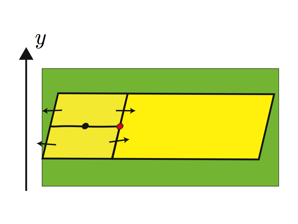
(b)
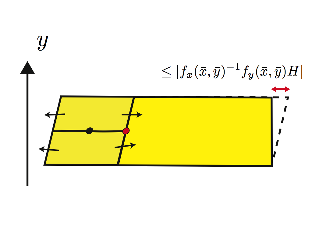
(c)
Figure 9: Cutting -cones (a) : A fast-saddle-type block with the basic form (Section 2.3.2) and associated unstable -cone. The union of yellow and white regions represents . The yellow region represents . The -components of block are identical for .
(b) : A fast-saddle-type block with the predictor-correctorc form (Section 2.3.3) and associated unstable -cone. The -components of the block as well as the cone are slid, since the -component of the center point also depends on ; . The fast-exit face thus has non-trivial angle to the -axis.
(c) : Cut the edge of unstable -cones. Resulting fast-exit face is parallel to the -axis. The length of the extended cone shortens at most , where is the height of the block in the -direction.
- Step 4.
-
Solve initial value problems of ODEs for setting a fast-exit-face of each block as an initial data and verify (CE4) in Definition 4.2 or Drop . This operation consists of direct applications of interval arithmetics and ODE solver libraries such as CAPD [3]. Although our computations here are operated in full systems, slow dynamics can be regarded as the small error since our interest in this step is mainly the behavior of fast dynamics.
Validation of assumptions in Lemma 4.39 in Step 2 can be done as follows.
Lemma 6.1 (Validation of assumptions in Lemma 4.39).
Let be a fast-saddle-type block with , and be an isolating block containing an equilibrium in the validated slow manifold with , where , and . Assume that satisfies the unstable -cone condition with
| (6.3) |
Also assume that can be chosen in
| (6.4) |
and that any subset containing is also an isolating block with the same isolating information as . Then we can choose an isolating block and the fast-exit face with and
| (6.5) |
so that assumptions in Lemma 4.39 holds.
Proof.
In practical computations, the most difficult part is Step 4. In general, the larger both the fast-exit face and the target -set in Drop, i.e., , are, the easier validations of covering relations are. However, if we validate covering relations described in Step 4, the resulting -sets is very close to the slow exit, i.e., (resp. ) in case that (resp. ). In particular, the next fast-exit face becomes too thin to validate the next Drop. Procedures in Step 2 as well as Step 4 thus looks incompatible each other. Nevertheless, an appropriate choice of the slow shadowing ratio avoids this inconsistency.
Lemma 6.2 (Validity of Step 2).
For each , consider the -th slow shadowing sequence in Step 2. Assume that a covering relation holds.
Let be the slow shadowing ratio satisfying
| (6.6) |
with .
Finally assume that is the slow shadowing sequence with the identical ratio . Then we can choose a fast-exit face so that (resp. ) in the case of (resp. ), where is an arbitrarily small number. As a consequence, Step 2 and Step 4 are valid simultaneously.
Proof.
We only prove the case . The case is similar.
By Proposition 4.14 with , we can construct a covering relation , where
The last equality follows from the choice of and in Step 2. Repeating this argument, two -sets describing the -th covering relation is located on and , respectively, where
We thus obtain . If the ratio can be chosen satisfying (6.6), we obtain
Consequently,
Obviously, the slow shadowing pair with the ratio satisfies the slow shadowing condition with the ratio for all . Therefore, arranging several ’s in the slow shadowing pair , we can take the -set on . Statements of the lemma follow from the same arguments as the proof of Proposition 4.15. Schematic pictures of the proof are shown in Fig. 10. ∎
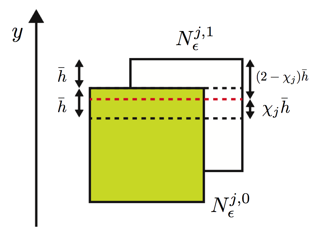
(a)
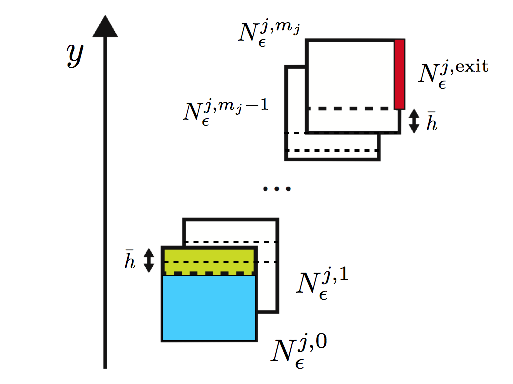
(b)
Dotted lines denote sections for each .
(a) : If the sequence of fast-saddle-type blocks is a slow shadowing sequence with the ratio ,
the section where the covering relation holds gets lower than the usual version ().
(b) : Repeating the procedure in (a) sufficiently many times, we can take the section before Jump at the bottom of ; namely, .
As a consequence, we can take the fast-exit face large keeping the target -set in Drop large.
Thanks to Lemma 6.2, we replace Step 2 by the following, which enables us to verify assumptions of results in Section 5 with large fast-exit faces and large target -sets in Drop:
- Step 2’
-
Replace the statement “verify the slow shadowing condition” in Step 2 by “verify the slow shadowing condition with the slow shadowing ratio ”, where is a given number satisfying (6.6).
If Steps 1, 2’, 3 and 4 pass, then all assumptions of either Theorem 5.1, Corollaries 5.3 or 5.4 are satisfied in the case of periodic orbits for all . Similarly, all assumptions of either Theorem 5.6, Corollaries 5.7 or 5.8 are satisfied in the case of heteroclinic or homoclinic orbits.
In Step 2, the predictor-corrector approach discussed in Section 2.3.3 is used for choosing local coordinates around (normally hyperbolic) invariant manifolds. A concrete form for validations is shown in Appendix A.
Note that all our examples below are cases . In such cases, one can directly verify covering relation by checking all assumptions in Proposition 2.9. In Step 4, we apply this proposition to validating covering relations.
We gather parameters we deal with computations in our settings except ones which arise in (6.1), before moving to practical computation examples. These parameters are set for each branch of slow manifolds which we try to find. Let be the number of branches.
- •
-
•
: The height of fast-saddle-type blocks in -direction. Each -interval of the length corresponds to the set in Section 2.3.2.
-
•
: A given number such that , where is the -component of an equilibrium . The equilibrium is computed numerically and becomes the center of the fast-saddle-type block ; the target -set of Drop.
-
•
: A given number such that , where is the -component of an equilibrium . The equilibrium is computed numerically and becomes the center of the fast-saddle-type block ; the last -set of the -th slow shadowing sequence containing a fast-exit face.
- •
-
•
: The length of spaces in fast-saddle-type blocks introduced in (4.3). For simplicity, these numbers are identical for all blocks. Moreover, they are assumed to be identical each other.
-
•
: Positive numbers less than introduced in (SS5).
-
•
: Positive numbers determining the sharpness of unstable and stable -cones, respectively.
-
•
: Positive numbers determining the length of unstable and stable -cones in (4.11) and (4.12), respectively. By using these numbers, we compute bounds of the departure time in (4.13) to construct the fast-exit face of the unstable -cone in (4.15), and the arrival time in (4.14). The arrival time is used to validate Drop to the target -set in the -direction corresponding to (4.16), as stated in Proposition 4.30.
All computations are done by MacBook Air 2011 model (1.6 GHz, Intel Core i5 Processor, 4GB Memory), GCC version 4.2.1 with -O2 option and CAPD library [3] version 3.0.
6.2 Demonstration 1 : slow shadowing sequences with the ratio
Validations of not only slow manifolds near critical manifolds consisting of equilibria for (1.3) but also the existence of trajectories which shadow slow manifolds are our starting points of whole considerations. Slow manifolds for (6.1) is now expected to be near the nullcline . The aim of this subsection is to test how large slow manifolds can be validated in terms of slow shadowing sequence. Following Step 2 at the beginning of this section, we validate slow shadowing sequences. Note that validations in this section also verify Jump in Proposition 4.15.
Computer Assisted Result 6.3.
Consider (6.1) with , and . Then for all and , the branch of slow manifolds near the nullcline in is validated. In particular, the slow shadowing condition with between blocks around this slow manifold is validated with parameters listed “First branch” in Table 1.
Similarly, the branch of slow manifolds near the nullcline in is validated. In particular, the slow shadowing condition with between blocks around this slow manifold is validated with parameters listed “Third branch” in Table 1.
| Parameters | First branch | Third branch |
|---|---|---|
| computation time | sec. | sec. |
This validation result implies that we have already validated trajectories with appropriately chosen initial data, say -sets, which shadow slow manifolds with an arbitrary length for all , as long as slow shadowing are validated. Moreover, Jump has been also validated for any fast-exit face with an appropriate height from the bottom (for ). The height can be explicitly determined from (6.6) in our setting. Remark that the range of our validating slow manifolds is not the limit of our verifications. Validations of slow shadowing sequences are just iterations of Step 2 and can be validated very fast, if we have fast solver of linear algebra. Notice that slow shadowing sequences for validate trajectories which shadow slow manifolds without solving any differential equations for all .
On the other hand, there is a trade-off for validating slow shadowing sequences. For example, if we raise the value of , say , the slow shadowing condition (4.5) violates, since the slow speed becomes faster than expansion and contraction of -sets in hyperbolic directions around slow manifolds. Factors determining (4.5) are , , , , , as well as eigenvalues and size of fast-saddle-type blocks. One expects that, the larger parameters, say , , are, the easier the validation of (4.5) will be. However, in such a case, the covering relation in Proposition 4.32 is often violated. In particular, Assumption (SS5) is violated. This is mainly because the distance between two centers and become larger and hence the affine map moves -sets larger, if we increase , , . This is also the case if we increase parameters and .
6.3 Demonstration 2 : -cones
Next, we show a demonstration of -cones. When we want to construct a covering-exchange sequence, we need to verify covering relation , where is a fast-exit face of a fast-saddle type block and is an other block. In order to verify this covering relation, we solve differential equation with the initial data . On the other hand, we can replace by a fast-exit face of an extended cone, thanks to discussions in Section 4.4. Here we solve (6.1) with two initial data, and , to see the following two points:
-
1.
accuracy of solution orbits, and
-
2.
verification of covering relations.
As an example, we set , , , and . These are parameter values used in Section 6.4. In demonstrating computations, we used the ODE solver in CAPD library based on Lohner’s method discussed in [38]. The order of Taylor expansion is set and time step size is set . Computation result is shown in Fig. 11.
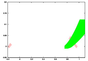
(a)
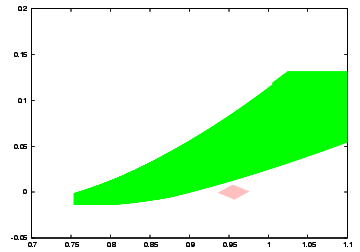
(b)
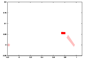
(c)
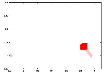
(d)
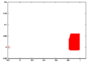
(e)
Horizontal axis: . Vertical axis: . Each figure represents the projection of trajectories and cones on -plane.
(a) Validation of solution orbits (green) with initial data . Pink regions are the union of fast-saddle-type blocks and extended cones. Computation step of ODEs is .
(b) The same computation result as (a). In this case the stable -cone is not validated. The tiny pink region around is the validated fast-saddle-type block. Readers see that enclosures of trajectories are much bigger than the fast-saddle-type block.
(c) Validation of solution orbits (red) with initial data (i.e. without unstable -cones) and the same time steps as (a). Validated trajectories do not arrive at target region yet.
(d) Validated trajectories with additional time step computations to (c). More precisely, computation step of ODEs is . Enclosures become bigger and bigger.
(e) Validated trajectories with additional time step computations to (d). More precisely, computation step of ODEs is . Enclosures are already bigger than stable cones, which implies that validation of covering relations can be never done.
First we compare the case we use stable -cones with the case we do not use stable -cones. Fig. 11-(a) and (b) show the same computational results. The only difference is whether or not a stable -cone is validated. In this example, we validate the stable -cone with the length of a fast-saddle-type block around (see Fig. 11-(a)). We solved ODE with initial data
after dividing it into uniform small pieces. Here denotes the fast-exit face of unstable -cone with the length of a fast-saddle type block around the origin in . In this example, we solved ODE in steps.
In general, validated fast-saddle type blocks corresponding to are very small, as shown in Fig. 11-(b) (colored by pink). On the other hand, validated trajectories are quite bigger than blocks. In our example, validated trajectories are already bigger than the block, which implies that we can never validate in this setting. A direct settlement of this problem would be a refinement of initial data, which leads to huge computational costs in many cases and is not realistic. Instead, we consider the problem with the help of stable -cones, which is shown in Fig. 11-(a). In this case, the target block corresponding to becomes big enough to validate covering relations. Thanks to Section 4.4, we can discuss validation of trajectories with extended cones, which is much easier than verifications without cones.
Next, we compare the case which we use unstable -cones with the case which we do not use unstable -cones. Computation result with unstable -cone is Fig. 11-(a). Figs. 11-(c), (d) and (e) show enclosure of trajectories with initial data , namely, a fast-exit face of a small fast-saddle-type block. If we do not use unstable -cones, we need to solve ODEs for longer time steps than the case we use unstable -cones (Fig. 11-(c)). Such extra computations cause additional computational errors and there is little hope to validate covering relations, as indicated in Figs. 11-(d), (e).
6.4 Periodic orbits
We go to validations of global orbits for (6.1). Our first example is validation of periodic orbits. As a demonstration we set , and and . All validation of covering-exchange sequences with extended cones yield the following computer assisted result.
Computer Assisted Result 6.4.
Consider (6.1) with , and . Then for all the following trajectories are validated.
-
1.
At , there is a singular heteroclinic chain consisting of
-
•
heteroclinic orbits from to , and from to ,
-
•
branches , of nullcline . contains and . Similarly, contains and .
Equilibria , , and are validated by
-
•
-
2.
For all , there exists a periodic orbit near .
Parameters for validations are listed in Table 2.
We omit computation times for slow shadowing and Jump, since they take only a few seconds as stated in Section 6.2.
| Parameters | On () | On () |
|---|---|---|
| (around ) | (around ) | |
| (around ) | (around ) | |
| (around ) | (around ) | |
| (around ) | (around ) | |
| (with ) | (with ) | |
| computation time | min. sec. | min. sec. |
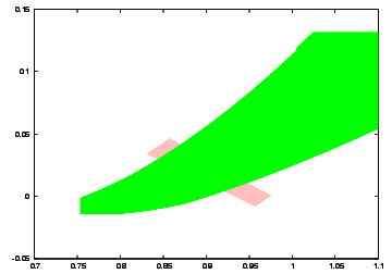
(a-1)
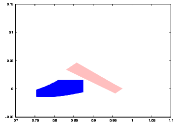
(a-2)
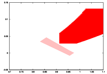
(a-3)
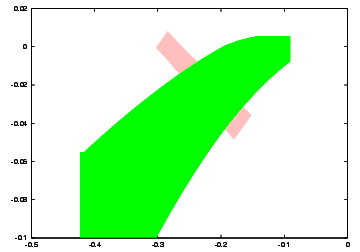
(b-1)
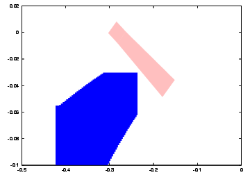
(b-2)
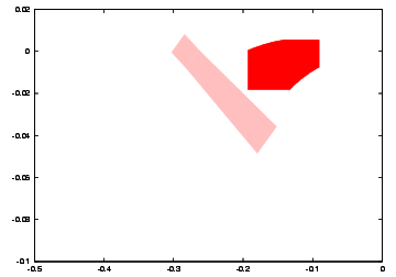
(b-3)
Horizontal axis: . Vertical axis: . Each figure represents the projection of trajectories and cones on -plane.
(a-1) : Validation of .
(a-2) : Validation of .
(a-3) : Validation of .
(b-1) : Validation of .
(b-2) : Validation of .
(b-3) : Validation of .
6.5 Heteroclinic cycles
The second example is a family of heteroclinic cycles. Consider the cubic curve . One can see that it is symmetric with respect to the inflection point
and we can choose from the curve to be the point that is symmetric to the origin with respect to the inflection point. Deng [8] shows that and with admit a heteroclinic loop of and for sufficiently small . Symmetry of the cubic curve with respect to implies that the vector field (6.1) with is symmetric under the following transformation:
It is thus sufficient to validate a heteroclinic orbit from the origin to if we want to validate heteroclinic cycles. Here we validate heteroclinic cycles for concrete and specific and . All validations of covering-exchange sequence with extended cones yield the following computer assisted result.
Computer Assisted Result 6.5.
Consider (6.1) with , , . Then, for , the following trajectories are validated.
-
1.
At , there is a singular heteroclinic chain consisting of
-
•
heteroclinic orbits from to , and from to ,
-
•
branches , of nullcline . contains and . Similarly, contains and .
Equilibria and are validated by
The equilibrium admits an attracting isolating block on contained in .
Note that is symmetric to with respect to the inflection point . Similarly, is symmetric to with respect to the inflection point .
-
•
-
2.
For all , there exists a heteroclinic cycle near . The cycle consists of heteroclinic orbits from to and from to .
Parameters for validations are listed in Table 3. Finally, assumptions of Lemma 6.1 are validated with the attracting isolating block on the slow manifold containing and the unstable -cone condition.
| Parameters | On () | On () |
|---|---|---|
| (around ) | ||
| (around ) | ||
| (around ) | ||
| (around ) | ||
| (with ) | ||
| computation time | min. sec. |
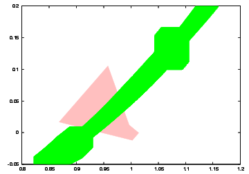
(a-1)
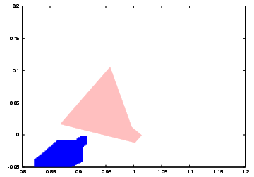
(a-2)
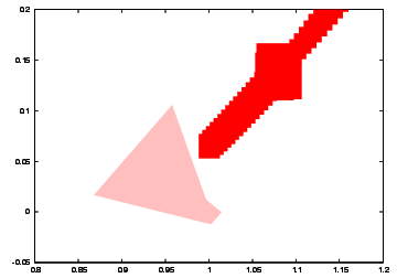
(a-3)
Horizontal axis: . Vertical axis: . Each figure represents the projection of trajectories and cones on -plane.
(a-1) : Validation of .
(a-2) : Validation of .
(a-3) : Validation of .
6.6 Heteroclinic orbits
The third example is a family of heteroclinic orbits which are different from heteroclinic cycles.
In this example we apply the method in Section 4.5 to isolating blocks on slow manifolds, which validates equilibria on slow manifolds.
Let be a point in such that and that . Assume that . Then there is a function which is unique in a small neighborhood of such that , and hold in such a neighborhood. This is due to the Implicit Function Theorem. Assuming that holds for all in a given neighborhood of , the above implicit function representation holds in the given neighborhood. By using implicit function differential, the vector field is rewritten by
near . Remark that . This expression leads to an effective estimate of vector fields on slow manifolds, as stated in Section 4.5.
All validation of slow shadowing sequences with extended cones and isolating blocks on slow manifolds yield the following computer assisted result.
Computer Assisted Result 6.6.
Consider (6.1) with , , .
-
1.
For each , the following two kinds of trajectories are validated:
-
(a)
At , there is a singular heteroclinic chain consisting of a heteroclinic orbit from to and a branch of nullcline connecting and . Equilibria have the following estimates:
-
(b)
For all , there exists a heteroclinic orbit from to near . The equilibrium admits an attracting isolating block on contained in .
Parameters for validations are listed in Table 4. Finally, assumptions of Lemma 6.1 are validated with the attracting isolating block on the slow manifold containing and the unstable -cone condition.
-
(a)
-
2.
For each , there exist the following two kinds of trajectories:
-
(a)
At , there is a singular heteroclinic chain consisting of a heteroclinic orbit from to and a branch of nullcline connecting and . Equilibria have the following estimates:
-
(b)
For all , there exists a heteroclinic orbit from to near . The equilibrium admits an attracting isolating block on contained in .
Parameters for validations are listed in Table 5. Finally, assumptions of Lemma 6.1 are validated with the attracting isolating block on the slow manifold containing and the unstable -cone condition.
-
(a)
In this case we have to care about the existence of an equilibrium on the slow manifold in . Easy calculations yield that possesses at most one equilibrium.
| Parameters | On () | On () |
|---|---|---|
| (around ) | ||
| (around ) | ||
| (around ) | ||
| (around ) | ||
| (with ) | ||
| computation time | min. sec. |
| Parameters | On () | On () |
|---|---|---|
| (around ) | ||
| (around ) | ||
| (around ) | ||
| (around ) | ||
| (with ) | ||
| computation time | min. sec. |
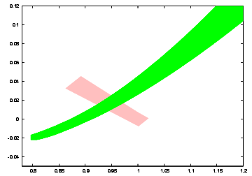
(a-1)
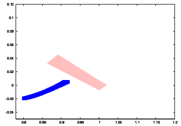
(a-2)
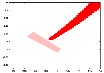
(a-3)
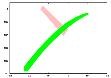
(b-1)
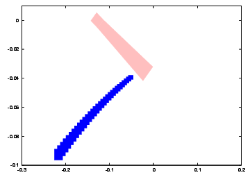
(b-2)
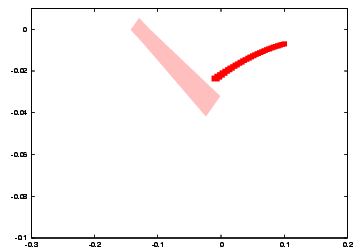
(b-3)
Horizontal axis: . Vertical axis: . Each figure represents the projection of trajectories and cones on -plane.
(a-1) : Validation of .
(a-2) : Validation of .
(a-3) : Validation of .
(b-1) : Validation of .
(b-2) : Validation of .
(b-3) : Validation of .
6.7 Homoclinic orbits
The final example is a family of homoclinic orbits. Set , , and . All validation of covering-exchange sequences with extended cones yield the following computer assisted result.
Computer Assisted Result 6.7.
Consider (6.1) with , and . Then for all the following trajectories are validated.
-
1.
At , there is a singular heteroclinic chain consisting of
-
•
heteroclinic orbits from to , and from to ,
-
•
branches , of nullcline . contains and . Similarly, contains and .
Equilibria , , and are validated by
-
•
-
2.
For all , there exists a homoclinic orbit of near . The equilibrium admits an attracting isolating block on contained in .
Parameters for validations are listed in Table 6. Finally, assumptions of Lemma 6.1 are validated with the attracting isolating block on the slow manifold and the unstable -cone condition.
| Parameters | On () | On () |
|---|---|---|
| (around ) | (around ) | |
| (around ) | (around ) | |
| (around ) | (around ) | |
| (around ) | (around ) | |
| (with ) | (with ) | |
| computation time | min. sec. | min. sec. |
Remark 6.8.
In this case we easily know that the only equilibrium of (6.1) for is and the dynamics around can be easily understood to show that is attracting on the slow manifold in .
Note that appropriate arrangements of computation schemes can improve the accuracy of validated trajectories and the validation range of parameters including .
In many articles, the uniqueness of global orbits is also discussed. From the geometrical viewpoint, typical arguments for the uniqueness require the transversality of locally invariant manifolds. In our cases, however, transversality in the sense of differential manifolds is not mentioned. In other words, we cannot prove the uniqueness of validated orbits in the current setting.
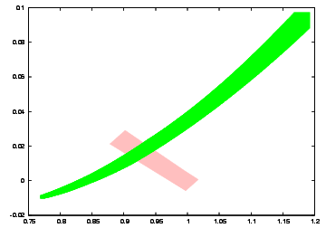
(a-1)
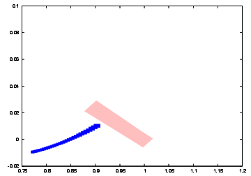
(a-2)
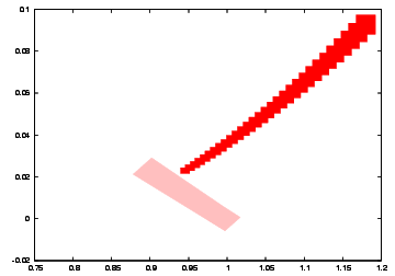
(a-3)
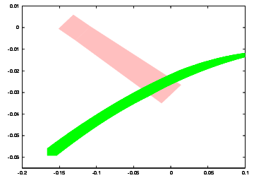
(b-1)
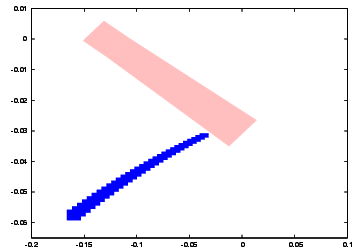
(b-2)
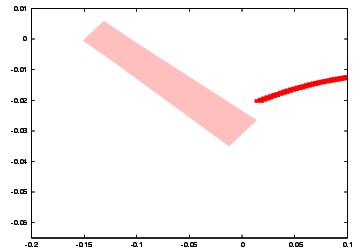
(b-3)
Horizontal axis: . Vertical axis: . Each figure represents the projection of trajectories and cones on -plane.
(a-1) : Validation of .
(a-2) : Validation of .
(a-3) : Validation of .
(b-1) : Validation of .
(b-2) : Validation of .
(b-3) : Validation of .
6.8 Continuation of homoclinic orbits
Finally, we verify the -continuation of homoclinic orbits validated in the previous subsection. It is very hard to validate trajectories of (6.1)ϵ for all with large at a time. In most cases, covering relations in the fast dynamics fail. To overcome this difficulty, we divide a closed interval into sub-intervals
and validate trajectories within each subinterval.
In our demonstrating example, we divide the interval into
Validating homoclinic orbits for each sub-interval and summarizing them, we obtain the following. Let and be points corresponding to those stated in Computer Assisted Result 6.7.
Computer Assisted Result 6.9.
The sharpness of unstable cones is an identical value : . The ratio in (4.5) are set as identical values : . The space length parameters of fast-saddle-type blocks are set as identical values : .
The sharpness of stable cones is an identical value : . The ratio in (4.5) are set as identical values : . The space length parameters of fast-saddle-type blocks are set as identical values : .
The sharpness of unstable cones is an identical value : . The ratio in (4.5) are set as identical values : for , for . The space length parameters of fast-saddle-type blocks are set as identical values : .
The sharpness of stable cones is an identical value : . The ratio in (4.5) are set as identical values : for , for . The space length parameters of fast-saddle-type blocks are set as identical values : .
| min. sec. | min. sec. | |
| min. sec. | min. sec. | |
| min. sec. | min. sec. | |
| min. sec. | min. sec. | |
| min. sec. | min. sec. | |
| min. sec. | min. sec. | |
| (Total) min. sec. | (Total) min. sec. |
It has taken about hours for validating Drop in in our computation environments. As for the slow shadowing and Jump, it totally takes less than seconds to validate.
Conclusion
We have proposed a topological methodology for validating singularly perturbed periodic, homoclinic and heteroclinic orbits for fast-slow systems with its applicability to concrete systems with computer assistance. The main features of our proposing methodology are the following.
-
•
Our central strategy consists of applications of well-known topological tools, covering relations, cones and isolating blocks, with taking the singular perturbation structure of normally hyperbolic invariant manifolds into account. This is one of different points from preceding works such as [1].
-
•
All our procedures can be validated via rigorous numerics (e.g. interval arithmetics). As a consequence, one can validate the continuation of singular limit orbits for all with a given with computer assistance.
A main concept for realizing the above points simultaneously is the covering-exchange; the singular perturbation’s version of covering relations. We have proposed not only its primitive form but also its generalization; a collection of local behavior named “slow shadowing”, “drop” and “jump”. The notion of covering-exchange describes the behavior of trajectories in the full system which shadow normally hyperbolic invariant manifolds as well as their stable and unstable manifolds, even for sufficiently small . In particular, this notion enables us to validate such trajectories without solving any differential equations in practical computations. Moreover, as mentioned above, it exceeds the limit of the multiple timescale parameter range: “sufficiently small ”, to with an explicit range in practical applications with computer assistance.
Of course, further applications of topological tools such as covering relations and the Conley index enable us to prove the existence of trajectories with complicated behavior. We believe that all these ideas will overcome difficulties of a broad class of singular perturbation problems.
We end this paper proposing further directions of our arguments.
- Bridging validation results to “direct” approach
Our methodology concentrates on validations of trajectories for on the basis of geometric singular perturbation theory. One of challenges concerning with continuation of trajectories is the integration of singularly perturbed trajectories with those by a direct approach; namely, validation of trajectories without taking account of singular perturbation structure of systems for positive bounded away from (e.g. [1]). In our validation examples, under a specific choice of parameter values, solution trajectories has been validated for in the case of homoclinic orbits for the FitzHugh-Nagumo system (6.1). In the case of (6.1), validations of each branch of slow manifolds are completed in less than one second.
This parameter range is still far from validation ranges with direct approaches; in [1], for example. Validations of slow shadowing for further range of are not easy, which is mainly because there is a trade-off between the slow shadowing condition (4.5) and the covering relation in Assumption (SS5), as discussed in Section 6.2. Both conditions are essential to describing slow shadowing, and hence our task for overcoming this situation will be developments of an improved topological and numerical method, like multi-step methods in numerical initial value problems, keeping the essence of slow shadowing phenomena. Obviously, if one can validate branches of normally hyperbolic slow manifolds by one blocks, there is no problem in this direction, in which case we can apply the primitive form of covering-exchange. After improvements of validations of slow shadowing or blocks containing slow manifolds with computer assistance, there will be a possibility that validated trajectories can be further continued in and, we hope, be connected to validated ones via direct approach under appropriate choice of various parameters or solvers. Further works in this direction from the viewpoint of topological and numerical analysis are ones of our future studies.
- Uniqueness and stability of validated orbits
In our topological theorems (Theorems 5.1, 5.6, Corollaries 5.3, 5.4, 5.7 and 5.8), only the existence of desiring orbits is stated. As for the uniqueness of such orbits, we have no answers yet. More precisely, these theorems only require topological transversality in terms of covering relations, which is weaker than the transversality in terms of differential manifolds. If we can even verify transversality in the sense of differential manifolds, then Exchange Lemma gives us the local uniqueness of singularly perturbed orbits. Transversality is also essential to discuss stability of connecting orbits. Jones [17] discusses stability of homoclinic orbits for (6.1) as the traveling wave solutions of FitzHugh-Nagumo PDE (6.2) from geometric viewpoints. For this stability arguments, some information about the nature of transversality between two manifolds play a central role.
One of standard approaches to transversality of manifolds is to use Melnikov integrals via solving variational equations. If we take rigorous numerics into account, the -Lohner method [38] provides the variational information of trajectories as well as solutions themselves and will give an answer to solve transversality problems.
- Covering-Exchange for fast-slow systems with multi-dimensional slow variables
Our validation arguments can be applied only to fast-slow systems with one-dimensional slow variable at present. It is natural to question whether our concept is applicable to fast-slow systems with multi-dimensional slow variables. The key problem concerning this extension is how we should track true trajectories near slow manifolds in terms of covering-exchange properties. Systems with multi-dimensional slow variables have rich behavior even on slow manifolds. The validation of slow manifolds by one fast-saddle-type block as well as concrete vector fields is thus more difficult than systems with one-dimensional slow variables because of nonlinearity of manifolds. It is not thus realistic to extend Theorem 5.1 and 5.6 to systems with multi-dimensional slow variable directly from the viewpoint of practical computations.
By the way, existence theorems of trajectories with covering relations imply that true trajectories shadow reference orbits. In the case of singular perturbation problems, reference orbits correspond to singular orbits consisting of heteroclinic orbits and trajectories on slow manifolds. Slow shadowing discussed in Section 4.3 reflects the aspect of shadowing trajectories in fast-slow systems with one-dimensional slow variable. This expectation will be valid even for systems with multi-dimensional slow variables. Such an extended sequence will yield the existence of true trajectories which shadow those on slow manifolds. Higher dimensional extension of slow shadowing condition or its analogue will give an explicit criterion for validations with rigorous numerics in reasonable processes.
- Extension of procedures for slow manifolds with non-hyperbolic points
Our validation arguments are based on the assumption that limiting critical manifolds are normally hyperbolic everywhere in consideration. Our procedure in this paper can be never applied if there is a point which is non-hyperbolic, like fold points, inside limiting critical manifolds. Nevertheless, there are a lot of cases that the interesting phenomena in singular perturbation problems are involved by such non-hyperbolic points. One of famous examples is canard solutions, which was discovered and first analyzed by Benoit, Callot, Diener and Diener [2]. A canard solution is a solution of a singular perturbed system which is contained in the intersection of an attracting slow manifold and a repelling one. Canard solutions provide a rich phenomenon such as canard explosion, namely, a transition from a small limit cycle to a relaxation oscillation through a sequence of canard cycles [9]. Since canard cycles involve fold points as jump points, our current implementations can never validate canard cycles. Krupa and Szmolyan [21] discuss the extension of geometric singular perturbation theory for slow manifolds including fold and canard points via the technique of blow-up. Simultaneously, Liu [22] discusses the Exchange Lemma in case that the critical manifold contains loss-of-stability turning points, corresponding the phenomenon called the delay of stability loss. In [22], the Fenichel-type coordinate which overcomes non-normal hyperbolicity is constructed by the other type of invariant manifold theorem proved by Chow-Liu-Yi [6]. We also mention sequential works by Schecter and Szmolyan [29, 27, 28, 30], which discuss the singularly perturbed Riemann-Dafermos solutions as the small perturbation of composite waves consisting of constant waves, shock waves and rarefaction waves in systems of conservation laws. There, non-hyperbolic points called gain-of-stability turning points naturally arise in invariant manifolds. They derive the General Exchange Lemma for describing behavior of tracking manifolds near such non-hyperbolic manifolds with the help of blow-ups.
We have to take such mathematical techniques into account, if we deal with invariant manifolds which are not normally hyperbolic with computer assistance.
Acknowledgements
This research was partially supported by Coop with Math Program, a commissioned project by MEXT, Japan. The author thanks to reviewers for providing him with helpful suggestions about contents and organizations of this paper.
References
- [1] G. Arioli and H. Koch. Existence and stability of traveling pulse solutions of the FitzHugh-Nagumo equation. Nonlinear Analysis: Theory, Methods & Applications, 113:51–70, 2015.
- [2] E. Benoit, J.L. Callot, F. Diener and M. Diener. Chasse au canards, Collect. Math., 31(1981), 37–119.
- [3] CAPD: Computer Assisted Proof of Dynamics software, http://capd.ii.uj.edu.pl
- [4] G.A. Carpenter. A geometric approach to singular perturbation problems with applications to nerve impulse equations. J. Differential Equations, 23(3):335–367, 1977.
- [5] R. Castelli and J.-P. Lessard. Rigorous numerics in Floquet theory: computing stable and unstable bundles of periodic orbits. SIAM J. Appl. Dyn. Syst., 12(1):204–245, 2013.
- [6] S.-N. Chow, W. Liu, and Y. Yi. Center manifolds for smooth invariant manifolds. Trans. Amer. Math. Soc., 352(11):5179–5211, 2000.
- [7] C. Conley. Isolated invariant sets and the Morse index, volume 38 of CBMS Regional Conference Series in Mathematics. American Mathematical Society, Providence, R.I., 1978.
- [8] B. Deng. The existence of infinitely many traveling front and back waves in the FitzHugh-Nagumo equations. SIAM J. Math. Anal., 22(6):1631–1650, 1991.
- [9] F. Dumortier and R. Roussarie. Canard cycles and center manifolds. Mem. Amer. Math. Soc., 121(577):x+100, 1996. With an appendix by Cheng Zhi Li.
- [10] N. Fenichel. Geometric singular perturbation theory for ordinary differential equations. J. Differential Equations, 31(1):53–98, 1979.
- [11] M. Gameiro, T. Gedeon, W. Kalies, H. Kokubu, K. Mischaikow, and H. Oka. Topological horseshoes of traveling waves for a fast-slow predator-prey system. J. Dynam. Differential Equations, 19(3):623–654, 2007.
- [12] R. Gardner and J. Smoller. The existence of periodic travelling waves for singularly perturbed predator-prey equations via the Conley index. J. Differential Equations, 47(1):133–161, 1983.
- [13] T. Gedeon, H. Kokubu, K. Mischaikow, and H. Oka. The Conley index for fast–slow systems. II. Multidimensional slow variable. J. Differential Equations, 225(1):242–307, 2006.
- [14] T. Gedeon, H. Kokubu, K. Mischaikow, H. Oka, and J.F. Reineck. The Conley index for fast-slow systems. I. One-dimensional slow variable. J. Dynam. Differential Equations, 11(3):427–470, 1999.
- [15] J. Guckenheimer, T. Johnson, and P. Meerkamp. Rigorous enclosures of a slow manifold. SIAM Journal on Applied Dynamical Systems, 11(3):831–863, 2012.
- [16] J. Guckenheimer and C. Kuehn. Computing slow manifolds of saddle type. SIAM J. Appl. Dyn. Syst., 8(3):854–879, 2009.
- [17] C.K.R.T. Jones. Stability of the travelling wave solution of the FitzHugh-Nagumo system. Trans. Amer. Math. Soc., 286(2):431–469, 1984.
- [18] C.K.R.T. Jones. Geometric singular perturbation theory. In Dynamical systems (Montecatini Terme, 1994), volume 1609 of Lecture Notes in Math., pages 44–118. Springer, Berlin, 1995.
- [19] C.K.R.T. Jones, T.J. Kaper, and N. Kopell. Tracking invariant manifolds up to exponentially small errors. SIAM J. Math. Anal., 27(2):558–577, 1996.
- [20] C.K.R.T. Jones and N. Kopell. Tracking invariant manifolds with differential forms in singularly perturbed systems. J. Differential Equations, 108(1):64–88, 1994.
- [21] M. Krupa and P. Szmolyan. Extending geometric singular perturbation theory to nonhyperbolic points—fold and canard points in two dimensions. SIAM journal on mathematical analysis, 33(2):286–314, 2001.
- [22] W. Liu. Exchange lemmas for singular perturbation problems with certain turning points. J. Differential Equations, 167(1):134–180, 2000.
- [23] K. Matsue. Rigorous numerics for stationary solutions of dissipative PDEs-Existence and local dynamics. Nonlinear Theory and Its Applications, IEICE, 4(1):62–79, 2013.
- [24] C.K. McCord. Mappings and homological properties in the Conley index theory. Ergodic Theory and Dynamical Systems, 8(8*):175–198, 1988.
- [25] K. Mischaikow. Conley index theory. In Dynamical systems (Montecatini Terme, 1994), volume 1609 of Lecture Notes in Math., pages 119–207. Springer, Berlin, 1995.
- [26] C. Robinson. Dynamical systems. Studies in Advanced Mathematics. CRC Press, Boca Raton, FL, second edition, 1999. Stability, symbolic dynamics, and chaos.
- [27] S. Schecter. Exchange lemmas 1: Deng’s lemma. Journal of Differential Equations, 245(2):392–410, 2008.
- [28] S. Schecter. Exchange lemmas 2: General exchange lemma. Journal of Differential Equations, 245(2):411–441, 2008.
- [29] S. Schecter and P. Szmolyan. Composite waves in the Dafermos regularization. Journal of Dynamics and Differential Equations, 16(3):847–867, 2004.
- [30] S. Schecter and P. Szmolyan. Persistence of rarefactions under Dafermos regularization: blow-up and an exchange lemma for gain-of-stability turning points. SIAM Journal on Applied Dynamical Systems, 8(3):822–853, 2009.
- [31] J. Smoller. Shock waves and reaction-diffusion equations, volume 258 of Grundlehren der Mathematischen Wissenschaften [Fundamental Principles of Mathematical Sciences]. Springer-Verlag, New York, second edition, 1994.
- [32] P. Szmolyan. Transversal heteroclinic and homoclinic orbits in singular perturbation problems. J. Differential Equations, 92(2):252–281, 1991.
- [33] S.-K. Tin, N. Kopell, and C.K.R.T. Jones. Invariant manifolds and singularly perturbed boundary value problems. SIAM J. Numer. Anal., 31(6):1558–1576, 1994.
- [34] J.B. van den Berg, J.D. Mireles-James, J.-P. Lessard, and K. Mischaikow. Rigorous numerics for symmetric connecting orbits: even homoclinics of the Gray-Scott equation. SIAM J. Math. Anal., 43(4):1557–1594, 2011.
- [35] D. Wilczak. The existence of Shilnikov homoclinic orbits in the Michelson system: a computer assisted proof. Found. Comput. Math., 6(4):495–535, 2006.
- [36] D. Wilczak. Abundance of heteroclinic and homoclinic orbits for the hyperchaotic Rössler system. Discrete Contin. Dyn. Syst. Ser. B, 11(4):1039–1055, 2009.
- [37] D. Wilczak and P. Zgliczyński. Topological method for symmetric periodic orbits for maps with a reversing symmetry. Discrete Contin. Dyn. Syst., 17(3):629–652 (electronic), 2007.
- [38] P. Zgliczyński. -Lohner algorithm. Found. Comput. Math., 2(4):429–465, 2002.
- [39] P. Zgliczyński. Covering relations, cone conditions and the stable manifold theorem. J. Differential Equations, 246(5):1774–1819, 2009.
- [40] P. Zgliczyński. Rigorous numerics for dissipative PDEs III. an effective algorithm for rigorous integration of dissipative PDEs. Topological Methods in Nonlinear Analysis, 36:197–262, 2010.
- [41] P. Zgliczyński and M. Gidea. Covering relations for multidimensional dynamical systems. J. Differential Equations, 202(1):32–58, 2004.
- [42] P. Zgliczyński and K. Mischaikow. Rigorous numerics for partial differential equations: the Kuramoto-Sivashinsky equation. Found. Comput. Math., 1(3):255–288, 2001.
Appendix A Concrete terms for (6.1) according to Section 2.3.3
Here we show concrete forms of error terms and Jacobian matrices calculated from the vector field (6.1) for validating fast-saddle-type blocks, and cone conditions with the predictor-corrector approach (Section 2.3.3).
A.1 Fast-saddle-type blocks
We list various terms in Section 2.3.3 in the case of FitzHugh-Nagumo system for readers’ accessibility. Let be a numerical zero of , where .
Use the coordinate given by the following:
| (A.1) |
where is a (numerical) root of and is assumed to be invertible. The transformed vector field as the extended system is then
where we introduced an auxiliary variable to be , , with constant .
The fast component of the vector field is
Denote (6.1) by
where and ; namely,
The Jacobian matrices at are
Around the numerical equilibrium , we introduce the affine transformation of the predictor-corrector form by
where is the nonsingular matrix such that . Then, denoting ,
Note that the linear order term of -variable in the error term is eliminated.
Let be an -set (in the -coordinate) containing . Then the Mean Value Theorem implies that the higher order term is included in the enclosure
Thanks to the term , this set is in general very small if is small. In our example, . Obviously, the first component is very small if is sufficiently small. Note that the denominator is bounded away from since we are focusing on validation of normally hyperbolic invariant manifolds. Finally, for given compact set and , we obtain enclosures of the error term
which can be computed by interval arithmetics and, in principle, returns very small enclosures for small and .
A.2 Jacobian matrices for cone conditions
The Jacobian matrix in this coordinate at ignoring the differential of -term is
| (A.2) |
where the variable in the second row corresponds to (A.1). We additionally transform linearly to by , where is the nonsingular matrix such that
The Jacobian matrix (A.2) in the new coordinate is then written as
| (A.3) | ||||
In order to verify cone conditions in a given -set containing , we compute corresponding maximal singular values in . All such calculations are done by interval arithmetics. As for calculations of the enclosure of in , it is useful to use the mean value form