Are tornado-like magnetic structures able to support solar prominence plasma?

Abstract

Recent high-resolution and high-cadence observations have surprisingly suggested that prominence barbs exhibit apparent rotating motions suggestive of a tornado-like structure. Additional evidence has been provided by Doppler measurements. The observations reveal opposite velocities for both hot and cool plasma on the two sides of a prominence barb. This motion is persistent for several hours and has been interpreted in terms of rotational motion of prominence feet. Several authors suggest that such barb motions are rotating helical structures around a vertical axis similar to tornadoes on Earth. One of the difficulties of such a proposal is how to support cool prominence plasma in almost-vertical structures against gravity. In this work we model analytically a tornado-like structure and try to determine possible mechanisms to support the prominence plasma. We have found that the Lorentz force can indeed support the barb plasma provided the magnetic structure is sufficiently twisted and/or significant poloidal flows are present.

1. Introduction

Recent high-resolution and high-cadence observations have revealed a possible rotating motion of prominence barbs around a vertical axis. These have been called barb tornadoes (Priest, 2014) due to the similarity of the apparent motion of such structures on the limb to terrestrial tornadoes. Su et al. (2012) reported an event where a prominence shows an apparent rotating motion with velocities of up to $8\,\mathrm{km\,s^{-1}}$. The observation shows cool prominence plasma seen in absorption in the $171$ Å passband of the SDO/AIA instrument. The authors argue that the motion is a rotation projected on the solar limb plane. However, such projected motions are also compatible with oscillations and counter-streaming flows, as pointed out by Panasenco et al. (2014). More events, up to 201 barb-tornadoes, have been reported by Wedemeyer et al. (2013) using AIA 171Å images. However, these authors studied mainly the morphology of the barbs and deduced a wide range of sizes and lifetimes.

Orozco Suárez et al. (2012) reported Doppler shifts using He I 1083.0 nm triplet data from the German Vacuum Tower Telescope (VTT) of the Observatorio del Teide (Tenerife, Spain). The observations revealed opposite velocities at the edges of the prominence feet of $\pm\,6\,\mathrm{km\,s^{-1}}$ along a slit placed close to the solar surface suggesting rotation of the cool prominence feet. The width of the feet is about $20\arcsec$ indicating a period of rotation of 4 hours.

More recently, Su et al. (2014) also reported Doppler shifts in a prominence pillar using the Fe XII 195Å line of the EIS instrument onboard the Hinode satellite. The observations revealed a bipolar velocity pattern along the whole vertical prominence pillar. The velocity is almost zero at the tornado axis and increases linearly up to $\sim\pm 5\,\mathrm{km\,s^{-1}}$ at the two edges of the observed structure. This indicates that also the million-degree plasma related to the tornado-like prominence may be rotating. The EUV bands of SDO/AIA reveal that the cool plasma seen in absorption moves in consort with the hot plasma. Additionally, Martínez-González et al. (2015), have found evidence of helical magnetic structure simultaneously at two prominence feet. All this evidence suggests that barb tornadoes are rotating vertical structures, nevertheless more observational evidence is needed.

The existence of such structures opens new questions concerning the origin of the tornado rotation and the influence of the rotating barb on the rest of the filament. Wedemeyer-Böhm et al. (2012) and Su et al. (2012) proposed that the barb-tornadoes are driven by photospheric vortex flows of the kind observed by Brandt et al. (1988) and Bonet et al. (2008): according to this view, the barb field lines are rooted in the vortices and the latter’s rotating motion is transferred to the barb. The authors also proposed that the barb tornadoes inject chromospheric plasma and helicity into the upper filament throughout the rotating barb. However, such vortex flows have yet not been observed at all below barbs, let alone as a matter of course.

Another possibility for the origin of spiral motions is three-dimensional reconnection (at or above the photosphere) during cancellation of photospheric magnetic fragments, since such reconnection will naturally produce vortex motions (e. g., Priest, 2014) and could also fuel a prominence with mass. A third possibility arises from the fact that a prominence represents a concentration of magnetic helicity in twisted magnetic fields. Thus, if part of a prominence dips down towards the photosphere, it is possible that such magnetic helicity and its associated twisting motions may be focused in the dip.

In this letter we discuss how the massive cool plasma is supported against gravity in a helical magnetic structure. We find that the barb-tornadoes bear many similarities to astrophysical plasma jets in which magneto-centrifugal forces accelerate the plasma. By using recent current tornado data and typical barb parameters we conclude that it is actually possible for the magnetic force to support and accelerate the cool barb plasma against gravity provided the structure is highly twisted and/or significant poloidal flows are present.

2. The barb-tornado model

Inspired by the observations, we consider in the following an axisymmetric model rotating around a vertical axis. We use cylindrical coordinates $(r,\varphi,z)$ with $z$ coinciding with the rotation axis. The axisymmetry condition implies that all quantities are $\varphi$-independent: $\partial/\partial\varphi=0$. An important restriction on the axisymmetric magnetic field is that the field lines should become vertical as we approach the rotation axis ($r\to 0$). The observed structure appears to be stationary with no important changes of shape in the EUV images and Doppler pattern for several hours. The Alfvén speed is around one thousand $\mathrm{km\,s^{-1}}$ in the corona and of order one hundred $\mathrm{km\,s^{-1}}$ in the cool prominence plasma. Thus, the travel time of a magnetic perturbation is less than a minute along the vertical axis of the tornado. This indicates that, during the few hours the observation, the system has plenty of time to relax and produce a stationary magnetic structure. We therefore set $\partial/\partial t=0$ in the equations. In this situation the MHD induction and momentum equations become, respectively,

$$0 = \nabla\times({\vec{v}}\times{\vec{B}})~{},$$ (1)

$$0 = -\rho({\vec{v}}\cdot\nabla){\vec{v}}-\nabla p+\frac{1}{{\mu_{0}}}(\nabla\times{\vec{B}})\times{\vec{B}}+\rho\vec{g}\,,$$ (2)

where $\rho$, ${\vec{v}}$, ${\vec{B}}$, $p$ and $\vec{g}=-g\vec{e}_{z}$ are the plasma density, the velocity, magnetic field, gas pressure and gravity respectively. Both the plasma velocity and magnetic field can be naturally decomposed into poloidal and toroidal components,

$${\vec{v}} = {\vec{v}}_{p}+v_{\varphi}\,{\vec{e}_{\varphi}}~{},$$ (3)

$${\vec{B}} = {\vec{B}}_{p}+B_{\varphi}\,{\vec{e}_{\varphi}}~{},$$ (4)

with ${\vec{v}}_{p}\cdot{\vec{e}_{\varphi}}={\vec{B}}_{p}\cdot{\vec{e}_{\varphi}}=0$. Only for illustration purposes we are showing in Figure 1 the force-free solutions of Schatzman (1965). The poloidal planes $(r,z)$ correspond to $\varphi=\mathrm{constant}$ surfaces. Given the axisymmetry, we can easily define the angular velocity $\Omega(r,z)$ using $\vec{v}_{\varphi}=r\,\Omega(r,z)\,{\vec{e}_{\varphi}}$. The advection (or inertial) term $({\vec{v}}\cdot\nabla){\vec{v}}$ can be written as

$$({\vec{v}}\cdot\nabla){\vec{v}}=(\vec{v}_{p}\cdot\nabla)\vec{v}_{p}-r\,\Omega^{2}\,\vec{e}_{r}+\frac{\vec{v}_{p}}{r}\cdot\nabla(r^{2}\Omega)\vec{e}_{\varphi}~{},$$ (5)

i.e., advection in the poloidal plane plus two acceleration terms associated with the prescribed rotation profile $\Omega(r,z)$, the first of which is clearly the centripetal force of a circular motion.

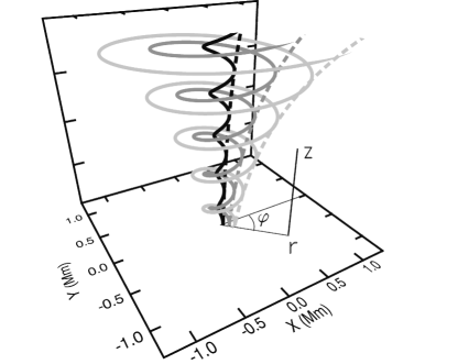
Figure 1.— Schematic picture of a tornado-like magnetic structure using the elementary force-free field of Schatzman (1965). Solid lines are the three dimensional representation of the magnetic field lines. Dashed lines are the poloidal field lines in the plane $\varphi=\mathrm{constant}$.

In a stationary regime there must be force balance including the inertial terms. For ease of notation, we use the symbol ${\vec{F}}_{nm}$ for the sum of pressure gradient, gravity and centrifugal force:

$${\vec{F}}_{nm}\;{\buildrel\scriptstyle def\over{=}}\;-\nabla p\;-\;\rho{{g}}{\vec{e}_{z}}\;+\;\rho r\Omega^{2}{\vec{e}_{r}}\;.$$ (6)

The poloidal part of the equation of motion (2) can then be split into into its components parallel and perpendicular to ${\vec{B}}_{p}$,

$$\frac{\rho}{2}\frac{\partial\,v_{p}^{2}}{\partial s} \;=\; {{\vec{F}}_{nm}}\cdot{\vec{e}_{\parallel}}-\frac{1}{2{\mu_{0}}r^{2}}\frac{\partial(rB_{\varphi})^{2}}{\partial s}~{},$$ (7)

$$0\; \;=\; \left[{\vec{F}}_{nm}-\nabla\frac{B_{p}^{2}}{2\,{\mu_{0}}}-\frac{1}{2\,\mu_{0}\,r^{2}}\nabla(rB_{\varphi})^{2}\right]\cdot{\vec{e}_{\perp}}$$ (8)

$$\;+\; \left(\frac{B_{p}^{2}}{{\mu_{0}}}-\rho\,v_{p}^{2}\right)\kappa_{pol}\;,$$

where ${\vec{e}_{\parallel}}$, ${\vec{e}_{\perp}}$ are the unit vectors in the poloidal plane parallel and perpendicular to ${\vec{B}}_{p}$, respectively, and $\kappa_{pol}$ and $s$ are the curvature and arc-length along the poloidal field lines (the latter is chosen such that ${\vec{e}_{\parallel}}$ points in the sense of growing $s$ illustrated as dashed lines in Fig. 1). For future reference, we also note that $v_{p}$ and $B_{p}$ are defined through ${\vec{v}}_{p}\cdot{\vec{e}_{\parallel}}$ and ${\vec{B}}_{p}\cdot{\vec{e}_{\parallel}}$, respectively, i.e., they can be positive or negative. Equation (7) represents the steady flow of plasma along field lines and provides clues concerning the support of the cool barb plasma; Equation (8) represents the global transverse equilibrium of the magnetic structure. The remaining component of the equation of motion, the azimuthal component, is

$$\rho\,({\vec{v}}_{p}\cdot\nabla)(r^{2}\,\Omega)\;=\;\left(\frac{{\vec{B}}_{p}}{\mu_{0}}\cdot\nabla\right)(r\,B_{\phi})\;.\\$$ (9)

As an additional remark concerning Figure 1, note that in a barb-tornado structure the density along the poloidal field lines should be larger close to the axis than in the outer regions of the structure. The observation of Su et al. (2014), which shows a dense column in absorption tapering off with height, may well be compatible with a helically opening structure as shown in the figure.

2.1. Pure Rotation

In a situation of pure rotation there is no plasma flow along the poloidal field (${\vec{v}}_{p}=0$), and the inertial term (5) reduces to the centripetal component $\,-\rho\,r\,\Omega^{2}\,{\vec{e}_{r}}\,$. In this case, from Equation (9), we see that the azimuthal component of the Lorentz force is zero, i.e., $rB_{\varphi}$ is constant along each poloidal field line. On the other hand, using the induction equation one can easily see that in this case $\Omega$ is constant along each given field line, in agreement with Ferraro’s isorotation law (Ferraro, 1937). The magnitudes of $rB_{\varphi}$ and $\Omega$ are then determined by the boundary conditions of the problem. Given the constancy of $rB_{\varphi}$, we see from the longitudinal equilibrium equation (7) that the Lorentz force has no longitudinal component, and so the equation reduces to

$${{\vec{F}}_{nm}}\cdot{\vec{e}_{\parallel}}=0\;.$$ (10)

The Lorentz force is thus purely poloidal and perpendicular to ${\vec{B}}_{p}$. Calling $\theta$ the angle between the poloidal field and the horizontal direction, equation (10) may be written

$$r\,\Omega^{2}\,\cos\theta-\frac{1}{\rho}\,\frac{\partial p}{\partial s}-\,{{g}}\,\sin\theta=0\;,$$ (11)

implying a balance of the non-magnetic forces. Note, in particular, that the centrifugal term could help support the plasma against gravity if the field lines are sufficiently close to horizontal (i.e., $\sin\theta>0$ sufficiently small).

Is the foregoing purely-rotating stationary equilibrium a realistic possibility for the observed apparent barb tornadoes? The latest observations (Su et al., 2014) reveal a rotational velocity of $5~{}\mathrm{km~{}s^{-1}}$ at the edges of the structure with $r=2\arcsec=1.5~{}\mathrm{Mm}$, so $\Omega\approx 3\times 10^{-3}~{}\mathrm{rad~{}s^{-1}}$. Wedemeyer et al. (2013) found average values of barb widths of $r\approx 2\arcsec$ in agreement with Su et al.. With these values we can compare the centrifugal acceleration to the gravitational acceleration,

$$\frac{r\,\Omega^{2}}{{{g}}}\approx 0.06=\tan(3.4\arcdeg)\;.$$ (12)

With the values found by Orozco Suárez et al. (2012) this ratio is even smaller. The only way to have centrifugal support of the plasma is then for the field lines to be almost horizontal, which contradicts the tornado picture. Can a pressure gradient help support the plasma in a non-horizontal field? Hot, coronal plasma, can be supported by a pressure gradient against gravity across coronal distances even in vertical field lines. However, for cool prominence plasma the pressure scale-height is too small to balance gravity in barbs as tall as those observed. Even if the field lines close to the rotation axis were filled with hot coronal plasma, the magnetic structure would have to turn almost horizontal (say, $3\arcdeg$, as given in Eq. 12) in the region holding cool prominence plasma. We conclude that the centrifugal force associated with the rotation cannot support the cool barb plasma against gravity in a helical field structure.

Another way to illustrate this conclusion is to estimate the rotational speed necessary to have purely centrifugal support, namely $v_{\varphi}=\sqrt{r{{g}}\tan\theta}\;.$ Assuming a magnetic field inclination of $45\arcdeg$, say, at the edges of the observed barb tornadoes, the rotation velocity would have to be $20~{}\mathrm{km~{}s^{-1}}$ if we use the data of Su et al. (2014) and $45~{}\mathrm{km~{}s^{-1}}$ when using those of Orozco Suárez et al. (2012), much larger than the measured speeds.

2.2. General case with poloidal flows

We consider now a more general scenario allowing for flows in the poloidal direction. Now the simple situation of constant $\Omega$ and $rB_{\varphi}$ along the field lines no longer applies. Checking for instance the azimuthal equation of motion (9), we see that a change of specific axial angular momentum of the plasma elements associated with the poloidal motion must be associated with a non-zero toroidal component of the Lorentz force, $({\vec{B}}_{p}/r)\cdot\nabla(r\,B_{\varphi})\,{\vec{e}_{\varphi}}$. Hence, in general $rB_{\varphi}$ can no longer be constant along field lines. In this situation, the Lorentz force also has a non-zero projection along poloidal field lines (Eq. 7), ${{F_{M}}_{long}}$,

$${{F_{M}}_{long}} {\buildrel\hbox{\tiny def}\over{=}} -\frac{1}{2{\mu_{0}}r^{2}}\frac{\partial(rB_{\varphi})^{2}}{\partial s}\;.$$ (13)

In spite of the added complication of this general scenario, there is a set of conserved quantities along the field lines. One can obtain them by following the general procedure used in the theory of astrophysical jets (Mestel, 1961; Lovelace et al., 1986). The induction equation requires that $\nabla\times({\vec{v}}_{p}\times{\vec{B}}_{p})=0$, so the poloidal velocity must be parallel to the poloidal field lines, for otherwise a singularity would arise in the toroidal electric field at the $z$-axis. So, we can write

$$\vec{v}_{p}=\kappa(r,z)~{}\vec{B}_{p}\;.$$ (14)

Integrating the MHD equations along field lines and simplifying the resulting expressions, a set of conserved quantities results, namely,

$${\mu_{0}}\rho\kappa = K~{},$$ (15)

$$\Omega-\frac{KB_{\varphi}}{{\mu_{0}}\rho\,r} = W~{},$$ (16)

$$\Omega r^{2}-\frac{rB_{\varphi}}{K} = \Lambda~{},$$ (17)

where $K$, $W$, and $\Lambda$ are all constant along each poloidal field line. Those relations allow us to find an explicit expression for $rB_{\varphi}$ along the poloidal field. One can write it in terms of the poloidal Alfvén Mach number

$${M_{A_{p}}^{2}}{\buildrel\hbox{\tiny def}\over{=}}\frac{v_{p}^{2}}{B_{p}^{2}/{\mu_{0}}\rho}=\frac{K^{2}}{{\mu_{0}}\rho}~{},$$ (18)

and of the Alfvén radius, $r_{A}$, defined by

$$r_{A}^{2}\;{\buildrel\hbox{\tiny def}\over{=}}\;\frac{\Lambda}{W}\;,$$ (19)

as follows:

$$rB_{\varphi} = KW\frac{r^{2}-r_{A}^{2}}{1-{M_{A_{p}}^{2}}}\;.$$ (20)

Expression (20) become singular when ${M_{A_{p}}^{2}}\to 1$. In the classical wind solutions, the flow speed increases from sub-Alfvenic to super-Alfvenic at a given point, and, to avoid the singularity, this transition must happen precisely at the Alfvén radius, $r=r_{A}$. In such models, this requirement serves as an internal boundary condition to pick up the desired trans-Alfvenic solution instead of the a completely sub-Alfvenic or completely super-Alfvenic solution. In our case, however, it is unlikely that the flows reach Alfvénic values within the tornado; rather, as shown below, we expect ${M_{A_{p}}^{2}}$ to remain below $1$ throughout.

Following Eq. (7) and the results of Section 2.1, to support the cool plasma along field lines the magnetic force ${{F_{M}}_{long}}$ of Eq. (13) should be larger than the centrifugal force, $f_{C}=\rho\,\Omega^{2}\,r$. From Eqs. (15) and (17), the ratio of these forces is

$$\left|\frac{{{F_{M}}_{long}}}{f_{C}}\right|=\left|\frac{T_{B}}{T_{v}}\right|\left(\frac{r}{L_{\Omega}}\right)\;,$$ (21)

in terms of the ratios ($T_{B}$ and $T_{v}$) of azimuthal to poloidal components for the magnetic fields and plasma velocities:

$$T_{B}{\buildrel\scriptstyle def\over{=}}\frac{B_{\varphi}}{B_{p}}\quad\hbox{and}\quad T_{v}{\buildrel\scriptstyle def\over{=}}\frac{v_{\varphi}}{v_{p}}\;,$$ (22)

and the length $L_{\Omega}$, defined as

$$L_{\Omega}=\left|\frac{\partial\ln(r^{2}\Omega)}{\partial s}\right|^{-1}\;.$$ (23)

The characteristic length (23) can be assumed to be of order the radial size of the system, i.e., $L_{\Omega}\sim\hbox{O(r)}$. Hence, from Equation (21), it is necessary for the value of the parameter $\left|T_{B}/T_{v}\right|$ to be large in order to have a barb-tornado dominated by the magnetic force. We see that a high level of magnetic twist, and a comparatively large poloidal velocity (compared to the rotational velocity) are necessary to provide magnetic support.

We can derive a more exact estimate of the possibilities of magnetic support of tornado plasma against gravity using expression (13) for the longitudinal magnetic force combined with expression (20). First of all, we can use the definitions of $W$ and $K$ to write their product in the form

$$K\,W={M_{A_{p}}^{2}}\frac{B_{p}}{r}\left(T_{v}-T_{B}\right)$$ (24)

keeping in mind, nevertheless, that $K$, $W$ (and $r_{A}$) are constant along each field line. We can now derive Eq. (20) with respect to the arc-length and, after a little algebra, obtain the general expression

$${{F_{M}}_{long}}\;=\;\frac{2}{r}\frac{B_{\varphi}\,B_{p}}{\mu_{0}}\frac{{M_{A_{p}}^{2}}}{1-{M_{A_{p}}^{2}}}\cos\theta\left[\,\left(1+\frac{\alpha}{2}\right)\,T_{B}-T_{v}\right]\,$$ (25)

where we have used $\cos\theta=\partial r/\partial s$, and called $\alpha$ the scale of variation of $\rho$ along poloidal field lines in terms of the cylindrical radius, as follows:

$$\alpha\quad{\buildrel\scriptstyle def\over{=}}\;\frac{r}{\cos\theta}\frac{\partial\log\rho}{\partial s}\;.$$ (26)

For the estimate that follows, it is best to write Equation (25) in terms of an observed quantity, namely $v_{\varphi}$, and of the ratio $T_{B}/T_{v}$, which turns out to be the essential dimensionless variable in the resulting expression. Further, to calibrate the possibilities of magnetic support, we normalize (25) with respect to gravity along the poloidal field, $\rho\,{{g}}\,\sin\theta$. The result is:

$$\frac{{{F_{M}}_{long}}}{\rho\,{{g}}\,\sin\theta}\quad = \quad\frac{2}{1-{M_{A_{p}}^{2}}}\;\left(\frac{v_{\varphi}^{2}}{{{g}}\,r}\right)\;\,\cdot\;$$ (27)

$$\left(\frac{T_{B}}{T_{v}}\right)\left[\,\left(1+\frac{\alpha}{2}\right)\,\frac{T_{B}}{T_{v}}-1\right]\cot\theta\,.$$

For the applications to prominence barbs we envisage cases with ${M_{A_{p}}^{2}}<1$. The term $1-{M_{A_{p}}^{2}}$ in Eq. 27 therefore favors magnetic support. In fact, in many cases ${M_{A_{p}}^{2}}\ll 1$ and so for simplicity this is the case we consider. Assuming the value of the ratio $v_{\varphi}^{2}/({{g}}\,r)$ to be given from observations expression (27) is basically a quadratic polynomial in $T_{B}/T_{v}$ with parameters $\alpha$ and $\theta$. In figure 2, we show (27) for $\theta=60\arcdeg$ (upper panel) and $\theta=20\arcdeg$ (lower panel), for different relevant values of $\alpha$. To draw the figure we have used $v_{\varphi}^{2}/({{g}}\,r)=0.06$ (i.e., $v_{\varphi}=5$ km s^-1 and $r=1.5$ Mm), which is the value that led us in Sec. 2.1, Equation 12, to conclude that there is no possible support for the plasma in the purely rotating case. For magnetic support, the relevant stretches of the curves are those near the dashed horizontal line at ordinate $=1$. For ease, we have marked the cut of each curve with that horizontal line with a large black dot and a thin dotted vertical line. The following guidelines have been used in the choice of values for $\alpha$: in a solar tornado $\alpha$ is probably negative, i.e., the density decreases as one goes outward along the tornado field lines. Also, $|\alpha|$ should not be larger than of order unity, since the lengthscale of variation of $\rho$ should be not too different from $r$ itself. Finally, in the figure we restrict ourselves to concave-upward parabolas (i.e, $\alpha>-2$), since those are the most favorable cases for magnetic support.

We see that it is not difficult to find values of $T_{B}/T_{v}$ that yield magnetic support of the plasma against gravity. In all cases shown, though, the basic variable $|T_{B}/T_{v}|$ must be above $1$: for $\theta=60\arcdeg$, for instance, the values marked in the figure range from $-6.3$ to $-3.3$, on the negative side and from $4.3$ to $7.3$ on the positive side. Note that the actual ranges are $[-14.2,-3.3]$ and $[4.3,\infty]$. For $\theta=20\arcdeg$, the absolute values are smaller. We expect $T_{v}$ to be perhaps $1$ or $2$, reflecting the fact that the outward motion of the tornado is possibly as fast as the rotating motion or a little less so. Thus, for magnetic support one would need a substantial level of magnetic twist, possibly $|B_{\varphi}/B_{p}|$ from a few to several units. If the poloidal flow becomes less important, then the amount of magnetic twist would increase to unrealistic values.

Figure 2.— Magnetic force along the field lines compared with the longitudinal component of gravity. For magnetic support, the value $1$ must be reached (marked by dots for the different curves)

3. Conclusions

In this work we have investigated a possible mechanism to support dense plasma in a prominence barb against gravity. We have modeled a barb tornado as an axisymmetric structure with rotation about the symmetry axis, in which the magnetic field is vertical close to the tornado axis. Pressure gradients are ruled out as a support for the plasma because the small pressure scale height of prominence plasma implies that they could support vertical structures only a few hundred kilometers tall, much smaller than the height of observed barbs.

In a barb tornado with a rotating helical field, extra magneto-centrifugal forces are present. We have found that the centrifugal force is much smaller than solar gravity for the barb-tornadoes observed so far. However, the poloidal magnetic force is a good candidate to support cool prominence plasma or even to inject such plasma into a prominence. For that, the structure must have significant magnetic twist and/or poloidal flows not much smaller than the rotational velocities. Whether this is or otherwise the case is a question for future observations. However, more theoretical work and observational evidence are needed to elucidate the origin of poloidal flows or magnetic twist.

References

- Bonet et al. (2008) Bonet, J. A., Márquez, I., Sánchez Almeida, J., Cabello, I., & Domingo, V. 2008, The Astrophysical Journal, 687, L131
- Brandt et al. (1988) Brandt, P. N., Scharmer, G. B., Ferguson, S., Shine, R. A., & Tarbell, T. D. 1988, Nature (ISSN 0028-0836), 335, 238
- Ferraro (1937) Ferraro, V. C. A. 1937, Monthly Notices of the Royal Astronomical Society, 97, 458
- Lovelace et al. (1986) Lovelace, R. V. E., Mehanian, C., Mobarry, C. M., & Sulkanen, M. E. 1986, Astrophysical Journal Supplement Series (ISSN 0067-0049), 62, 1
- Martínez-González et al. (2015) Martínez González, M. J., Manso Sainz, R., Asensio Ramos, A., et al. 2015, ApJ, 802, 3
- Mestel (1961) Mestel, L. 1961, Monthly Notices of the Royal Astronomical Society, 122, 473