Elasticity and Glocality: Initiation of Embryonic Inversion in Volvox

Abstract

Elastic objects across a wide range of scales deform under local changes of their intrinsic properties, yet the shapes are glocal, set by a complicated balance between local properties and global geometric constraints. Here, we explore this interplay during the inversion process of the green alga Volvox, whose embryos must turn themselves inside out to complete their development. This process has recently been shown [S. Höhn et al., Phys. Rev. Lett. 114, 178101, (2015)] to be well described by the deformations of an elastic shell under local variations of its intrinsic curvatures and stretches, although the detailed mechanics of the process have remained unclear. Through a combination of asymptotic analysis and numerical studies of the bifurcation behavior, we illustrate how appropriate local deformations can overcome global constraints to initiate inversion.

I Introduction

The shape of many a deformable object arises through the competition of multiple constraints on the object: this competition may be between different global constraints, such as in Helfrich’s analysis helfrich of the shape of a red blood cell (where intrinsic curvature effects coexist with constrained membrane area and enclosed volume). It may also be the competition between local and global constraints. Such deformations, which we shall term glocal, arise for example in origami patterns silverberg (where local folds must be compatible with the global geometry). They are of considerable interest in the design of programmable materials bende at macro- and microscales, where one asks: can a sequence of local deformations overcome global constraints and direct the global deformations of an object?

This is a problem that, at the close of their development, the embryos of the green alga Volvox kirkbook are faced with in the ponds of this world. Volvox (Fig. 1a) is a multicellular green alga belonging to a lineage (the Volvocales) which has been recognized since the time of Weismann Weismann as a model organism for the evolution of multicellularity, and which more recently has emerged as the same for biological fluid dynamics ARFM . The Volvocales span from unicellular Chlamydomonas, through organisms such Gonium, consisting of $8$ or $16$ Chlamydomonas-like cells in a quasi-planar arrangement, to spheroidal species (Pandorina and Pleodorina) with scores or hundreds of cells at the surface of a transparent extracellular matrix (ECM). The largest members of the Volvocales are the species of Volvox, which display germ-soma differentiation, having sterile somatic cells at the surface of the ECM and a small number of germ cells in the interior which develop to become the daughter colonies.

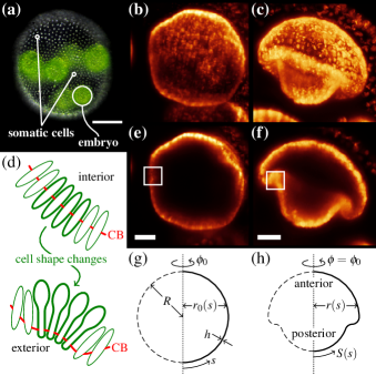
Figure 1: (color online). Volvox invagination and elastic model. (a) Adult Volvox, with somatic cells and one embryo labelled. (b) Volvox embryo at the start of inversion. (c) Mushroom-shaped invaginated Volvox embryo. (d) Cell shape changes to wedge shapes and motion of cytoplasmic bridges (CB) bend the cell sheet. Red line indicates position of cytoplasmic bridges. (e,f) Cross-sections of the stages shown in panels (b,c). Cell shape changes as in (d) occur in the marked regions. (g) Geometry of undeformed spherical shell of radius $R$ and thickness $h$. (h) Geometry of deformed shell. Scale bars: (a) $50\,\mbox{\textmu m}$, (e,f) $20\,\mbox{\textmu m}$. False color images obtained from light-sheet microscopy provided by Stephanie Höhn and Aurelia R. Honerkamp-Smith.

Following a period of substantial growth, the germ cells of Volvox undergo repeated rounds of cell division, at the end of which each embryo (Fig. 1b,e) consists of a few thousand cells arrayed to form a thin spherical sheet kirkbook . These cells are connected to each other by the remnants of incomplete cell division, thin membrane tubes called cytoplasmic bridges kirk81_1 ; kirk81_2 . The ends of the cells whence emanate the flagella, however, point into the sphere at this stage, and so the ability to swim is only acquired once the alga turns itself inside out through an opening at the top of the cell sheet, called the phialopore viamontes77 ; kirkreview ; hallmann .

Of particular interest in the present context is the crucial first step of this process, the formation of a circular invagination in so-called ‘type B’ inversion (Fig. 1c,f) followed by the engulfing of the posterior by the anterior hemisphere hallmann ; hohn11 . (This scenario is distinct from ‘type A’ inversion in which the initial steps involve four lips which peel back from a cross-shaped phialopore.) The invaginations of cell sheets found in type B inversion are very generic deformations during morphogenetic events such as gastrulation and neurulation he ; lowery ; eiraku ; sawyer , but, in animal model organisms, they often arise from an intricate interplay of cell division, intercalation, migration and cell shape changes. Modelling these therefore requires cell-based models, as pioneered by Odell et al. odell , but simpler models of simpler morphogenetic processes are required to elucidate the underlying mechanics of these problems howard . Inversion in Volvox is, however, driven by active cell shape changes alone: inversion starts when cells close to the equator of the shell elongate and become wedge-shaped hohn11 . Simultaneously, the cytoplasmic bridges migrate to the wedge ends of the cells, thus splaying the cells locally and causing the cell sheet to bend hohn11 (Fig. 1d). Additional cell shape changes have been implicated in the relative contraction of one hemisphere with respect to the other in order to facilitate invagination hohn14 . After invagination, the bend region expands, allowing the posterior hemisphere to invert fully.

At a more physical level, it has been shown recently that the inversion process is simple enough to be amenable to a mathematical description hohn14 : the deformations of the alga are well reproduced by a simple elastic model in which the cell shape changes and motion of cytoplasmic bridges impart local variations of intrinsic curvature and stretches to an elastic shell hohn14 . The associated mechanics have remained unclear, however. Here, we perform an asymptotic analysis at small deformations to clarify the geometric distinction between deformations resulting from intrinsic bending and intrinsic stretching, respectively. A numerical study of the bifurcation behavior further serves to illustrate how a sequence of local deformations can achieve invagination, and how contraction complements bending in this picture.

II Elastic Model

Following Höhn et al. hohn14 , we inscribe Volvox inversion into the very general framework of the axisymmetric deformations of a thin elastic spherical shell of radius $R$ and thickness $h\ll R$ under variations of its intrinsic curvature and stretches. The undeformed, spherical, configuration of the shell is characterized by arclength $s$ and the distance of the shell from its axis of revolution, $r_{0}(s)$ (Fig. 1g). To these correspond arclength $S(s)$ and distance from the axis of revolution $r(s)$ in the deformed configuration (Fig. 1h). The undeformed and deformed configurations are related by the meridional and circumferential stretches,

$$f_{s}(s)=\frac{\mathrm{d}S}{\mathrm{d}s}\ \ \ \ \ \ {\rm and}\ \ \ \ \ \ f_{\phi}(s)=\frac{r(s)}{r_{0}(s)}~{}.$$ (1)

(These definitions do not require that the undeformed configuration be spherical, and apply for the deformations of any axisymmetric object.) These define the strains

$$E_{s}=f_{s}-f_{s}^{0}, E_{\phi}=f_{\phi}-f_{\phi}^{0},$$ (2)

and curvature strains

$$K_{s}=f_{s}\kappa_{s}-f_{s}^{0}\kappa_{s}^{0}, K_{\phi}=f_{\phi}\kappa_{\phi}-f_{\phi}^{0}\kappa_{\phi}^{0},$$ (3)

where $\kappa_{s}$ and $\kappa_{\phi}$ denote the meridional and circumferential curvatures of the deformed shell. The intrinsic curvatures and stretches introduced by $f_{s}^{0},f_{\phi}^{0}$ and $\kappa_{s}^{0},\kappa_{\phi}^{0}$ extend Helfrich’s work on membranes helfrich . The deformed configuration of the shell minimises an energy of the Hookean form libai ; audolypomeau ; knoche11

$$\mathcal{E} =\dfrac{\pi Eh}{1-\nu^{2}}\int_{0}^{\pi R}{r_{0}\Bigl{(}E_{s}^{2}+E_{\phi}^{2}+2\nu E_{s}E_{\phi}\Bigr{)}\,\mathrm{d}s}$$

$$\hskip 14.22636pt+\dfrac{\pi Eh^{3}}{12(1-\nu^{2})}\int_{0}^{\pi R}{r_{0}\Bigl{(}K_{s}^{2}+K_{\phi}^{2}+2\nu K_{s}K_{\phi}\Bigr{)}\,\mathrm{d}s}.$$ (4)

with material parameters the elastic modulus $E$ and Poisson’s ratio $\nu$. In computations, we take $h/R=0.15$ and $\nu=1/2$ appropriate for Volvox inversion hohn14 .

In general, deformations of the shell arise from a complex interplay of intrinsic stretches and curvatures, and the global geometry of the shell. To clarify these, we begin by considering two simple kinds of deformations, in which the competition is between two effects only. How these effects conspire in general we shall explore in the main body of the paper.

II.0.1 Simple Deformations: Stretching and Bending

The simplest intrinsic deformation is one of uniform stretching or contraction, which does not affect the global, spherical geometry of the shell. This corresponds to $f_{s}^{0}=f_{\phi}^{0}=f$ and $\kappa_{s}^{0}=\kappa_{\phi}^{0}=1/fR$. With these intrinsic stretches and curvatures, the original sphere deforms to a sphere of radius $R^{\prime}$. Then $f_{s}=f_{\phi}=R^{\prime}/R$, and so the strains are $E_{s}=E_{\phi}=R^{\prime}/R-f$. However, $\kappa_{s}=\kappa_{\phi}=1/R^{\prime}$. Thus $f_{s}\kappa_{s}=f_{\phi}\kappa_{\phi}=f_{s}^{0}\kappa_{s}^{0}=f_{\phi}^{0}\kappa_{\phi}^{0}=1/R$, and so $K_{s}=K_{\phi}=0$. The energy density is therefore proportional to $(R^{\prime}/R-f)^{2}$ and is minimized for $R^{\prime}=fR$, at which point $\mathcal{E}=0$ (Fig. 2a). (Indeed, uniform contraction is a homothetic transformation: the angles between material points are unchanged, and so there is no bending involved. In other words, the shell is blind to its intrinsic curvature on this spherical solution branch.)

The intrinsic stretches and curvatures need not be compatible in this way, however: suppose that $f_{s}^{0}=f_{\phi}^{0}=f$, but $\kappa_{s}^{0}=\kappa_{\phi}^{0}=1/f^{\prime}R$ with $f\not=f^{\prime}$. The energy still has spherical minima of radius $R^{\prime}=fR$, but now with $\mathcal{E}\not=0$ (Fig. 2a). This illustrates that, conversely, even if the equilibrium shape is spherical, the intrinsic curvatures and stretches cannot straightforwardly be inferred from the resulting shape.

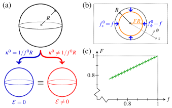
Figure 2: (color online). Simple intrinsic deformations. (a) A sphere can be shrunk to smaller spheres of equal radii by both compatible and incompatible intrinsic deformations. (b) Contraction of a circular region of radius $R$ in a plane elastic sheet by a factor $f$. The boundary of this region is contracted to $s=FR$. (c) Numerical result for $F$ (+) agrees with analytical calculation (13) (solid line).

II.0.2 Simple Deformations: Stretching and Geometry

To illustrate how the global geometry affects these deformations, we consider contraction of a plane elastic sheet, with $f_{s}^{0}=f_{\phi}^{0}=f<1$ for $s<R$ (Fig. 2b). This does not involve any bending of the sheet, and, upon non-dimensionalising lengths with $R$, the shell minimises

$$\int_{0}^{\infty}{s\Bigl{\{}\bigl{[}r^{\prime}(s)-f(s)\bigr{]}^{2}+\bigl{[}r(s)/s-f(s)\bigr{]}^{2}}$$

$$\hskip 42.67912pt+2\nu\bigl{[}r^{\prime}(s)-f(s)\bigr{]}\bigl{[}r(s)/s-f(s)\bigr{]}\Bigr{\}}\,\mathrm{d}s,$$ (5)

where

$$f(s)=\left\{\begin{array}[]{cl}f&\text{if }s<1\\ 1&\text{if }s>1.\end{array}\right.$$ (8)

The resulting Euler–Lagrange equation is

$$\dfrac{\mathrm{d}}{\mathrm{d}s}\left(s\dfrac{\mathrm{d}r}{\mathrm{d}s}\right)-\dfrac{r}{s}=(1+\nu)(1-f)s\,\delta(s-1).$$ (9)

This is a homogeneous equation, and the solution satisfying the geometric conditions $r(0)=0$ and $r(s)\sim s$ as $s\rightarrow\infty$ as well as continuity of $r$ at $s=1$ is

$$r(s)=\left\{\begin{array}[]{cl}Fs&\text{if }s<1\\ s+\dfrac{F-1}{s}&\text{if }s>1.\end{array}\right.$$ (12)

The constant $F=r(1)$ is determined by the jump condition at $s=1$, or, physically, by requiring the stress to be continuous across $s=1$. This finally yields

$$F=\dfrac{1}{2}\left[(1-\nu)+(1+\nu)f\right].$$ (13)

This simplified problem serves as a test case for numerical solution of the more general Euler–Lagrange equations associated with (4). These boundary-value problems can be solved numerically with the solver bvp4c of Matlab (The Mathworks, Inc.); our numerical setup of the governing equations otherwise mimicks that of knoche11 . In this particular example, the linear relationship in (13) is indeed confirmed numerically (Fig. 2c). Notice that the governing equation (9) is independent of the forcing applied away from $s=1$; the solution is determined by geometric boundary conditions.

III Results

The most drastic cell shape changes at the start of inversion occur when cells in a narrow region close to the equator become wedge-shaped (Fig. 1d). These are accompanied by motion of the cytoplasmic bridges to the thin tips of the cells to splay the cell sheet and drive its inward bending. For this reason, Höhn et al. hohn14 started by considering a piecewise constant functional form for the intrinsic curvature, in which this curvature took negative values in a narrow region close to the equator. It was found, however, that with this ingredient alone the energy minimizers could not reproduce the mushroom shapes adopted by the embryos in the early of stages of inversion (Fig. 1c,f), producing instead a shape cinched in at those points – the so-called ‘purse-string’ effect. However, analysis of thin sections had previously revealed that the cells in the posterior hemisphere become thinner at the start of inversion hohn11 . When the resulting contraction of the posterior hemisphere was incorporated into the model, it could indeed reproduce, quantitatively, the shapes of invaginating Volvox embryos.

Höhn et al. have thus identified two different types of active deformations that contribute to the shapes of inverting Volvox at the invagination stage: first, a localized region of active inward bending (corresponding to negative intrinsic curvature), and second, relative contraction of one hemisphere with respect to the other. We shall focus on these two types of deformation in what follows and clarify the ensuing elastic and geometrical balances.

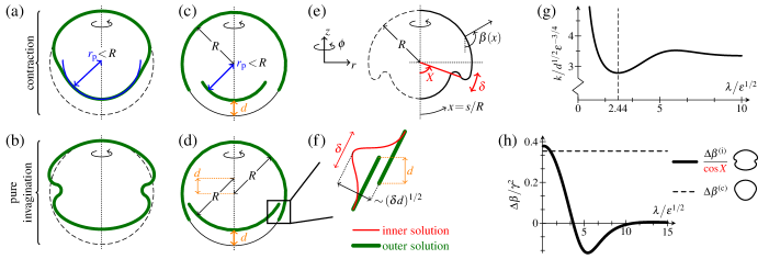
Figure 3: (color online). Asymptotic analysis of invagination and contraction. (a) Numerical shape resulting from contracting the posterior to a radius $r_{\mathrm{p}}<R$. (b) Numerical “hourglass” shape resulting from pure invagination. (c) Geometry of contraction with posterior radius $r_{\mathrm{p}}<R$, resulting in upward motion of the posterior by a distance $d$. (d) Geometry of pure invagination solution. (e) Asymptotic geometry: in the limit $h\ll R$, deformations are localized to an asymptotic inner layer of width $\delta$ about $x=X$, where $x=s/R$ is the angle that the undeformed normal makes with the vertical. In the deformed configuration, this angle has changed to $\beta(x)$. (f) Asymptotic invagination: upward motion of posterior by a distance $d$ requires inward deformations scaling as $(\delta d)^{1/2}$ in the inner layer of width $\delta$. (g) Relation between preferred curvature $k$ and width of invagination $\lambda$ for a given amount of upward posterior motion $d$, from asymptotic calculations. (h) Inward rotation of midpoint of invagination with, and without contraction, from asymptotic calculations.

III.1 Asymptotic Analysis

We start by seeking equilibrium configurations in the limit of a thin shell, $h\ll R$. In this limit, the shapes (Fig. 3a,b) corresponding to contraction or (pure) invagination (by which we mean, here, deformations driven by a region of high intrinsic curvature only) result from the matching of spherical shells of different radii or disparate relative positions (Fig. 3c,d). Deviations from these outer solutions are localized to an asymptotic inner layer of non-dimensional width $\delta$ about $x=X$, where $x=s/R$ is the angle that the normal to the undeformed shell makes with the vertical (Fig. 3e). Here, we consider an incipient deformation where the normal angle $\beta(x)$ to the deformed shell deviates but slightly from its value in the spherical configuration, viz $\beta(x)=x+b(x)$, with $b\ll 1$.

III.1.1 Geometric Considerations

We begin by clarifying the geometric distinction between contraction and invagination. The radial and vertical displacements obey

$$u_{r}^{\prime} =f_{s}\cos{\beta}-\cos{x}=-b\sin{X}+O\bigl{(}\delta b,b^{2}\bigr{)},$$ (14a)

$$u_{z}^{\prime} =f_{s}\sin{\beta}-\sin{x}=b\cos{X}+O\bigl{(}\delta b,b^{2}\bigr{)},$$ (14b)

where dashes denote differentiation with respect to $x$, and where we have assumed the scaling $f_{s}=1+O(\delta b)$ which we shall derive presently. Let $d$ denote the (non-dimensional) distance by which the posterior moves up. Matching to the outer solutions requires the net displacements $U_{r}$ and $U_{z}$, obtained by integrating (14) across the inner layer, to obey

$$U_{r}^{\text{(c)}} =d\sin{X}, U_{z}^{\text{(c)}} =-d\cos{X},$$ (15a)

$$U_{r}^{\text{(i)}} =0, U_{z}^{\text{(i)}} =-d,$$ (15b)

where the superscripts (c) and (i) refer, respectively, to the solutions corresponding to contraction and (pure) invagination. In the case of contraction, (14) and (15a) give the scaling $b^{\text{(c)}}\sim d/\delta$. If there is no contraction, however, (14) and (15b) imply that the leading-order solution does not yield any upward motion of the posterior, which is associated with a higher-order solution only. This suggests that the appropriate scaling is $b^{\text{(i)}}\sim(d/\delta)^{1/2}$, which we shall verify presently.

Our assumption $b\ll 1$ thus translates to $d\ll\delta$. Hence, in the invagination case, upward motion of the posterior requires comparatively large inward displacements of order $(\delta d)^{1/2}\gg d$ (Fig. 3f). This asymptotic difference of the deformations corresponding to contraction and invagination arises purely from geometric effects; it is the origin of the ‘purse-string’ shapes found by Höhn et al. in the absence of contraction hohn14 .

III.1.2 Elasto-Geometric Considerations

Here, we discuss the detailed solution for pure invagination. Upon non-dimensionalising distances with $R$ and stresses with $Eh$, the Euler–Lagrange equations of (4), derived in the appendix, can be cast into the form

$$f_{s}\mathit{\Sigma}\sin{x}\tan{\beta}-\varepsilon^{2}\cos{\beta}\Bigl{(}1-\nu\beta^{\prime}-\sin{\beta}\operatorname{cosec}{x}\Bigr{)}$$

$$\hskip 17.07164pt-\varepsilon^{2}\dfrac{\mathrm{d}}{\mathrm{d}x}\Bigl{(}\beta^{\prime}\sin{x}+\nu\bigl{(}\sin{\beta}-\sin{x}\bigr{)}\Bigr{)}=k^{0}(x),$$ (16a)

$$\dfrac{\mathrm{d}}{\mathrm{d}x}\Bigl{(}\mathit{\Sigma}\sec{\beta}\sin{x}\Bigr{)}-A-\nu\mathit{\Sigma}=0,$$ (16b)

with the small parameter

$$\varepsilon^{2}=\dfrac{1}{12(1-\nu^{2})}\dfrac{h^{2}}{R^{2}}\ll 1.$$ (17)

In these equations, $\mathit{\Sigma}$ is the non-dimensional meridional stress, and $A=e_{\phi}$ is the dimensionless hoop strain. The contribution from the intrinsic curvature is

$$k^{0}(x)=\varepsilon^{2}\left\{\nu\kappa_{s}^{0}(x)\cos{\beta}-\dfrac{\mathrm{d}}{\mathrm{d}x}\Bigl{(}\kappa_{s}^{0}\sin{x}\Bigr{)}\right\}.$$ (18)

The equations are closed by the geometric relation

$$\dfrac{\mathrm{d}}{\mathrm{d}x}\Bigl{(}A\sin{x}\Bigr{)}=f_{s}\cos{\beta}-\cos{x}.$$ (19)

Introducing $\gamma=(d/\delta)^{1/2}$, scaling gives the leading balances $\mathit{\Sigma}\sim\varepsilon^{2}\gamma/\delta^{2}$, $\mathit{\Sigma}/\delta\sim A$, and $A/\delta\sim\gamma$ in (16,19). Hence $\delta\sim\varepsilon^{1/2}$, and we define an inner coordinate $\xi$ via $x=X+\delta\xi$. We also introduce the expansions

$$\beta =X+\gamma\bigl{(}b_{0}+\gamma b_{1}+\gamma^{2}b_{2}+\cdots\bigr{)},$$ (20a)

$$A =\delta\gamma\bigl{(}a_{0}+\gamma a_{1}+\cdots\bigr{)},$$ (20b)

$$\mathit{\Sigma} =\delta^{2}\gamma\cot{X}\bigl{(}\sigma_{0}+\gamma\sigma_{1}+\cdots\bigr{)}.$$ (20c)

This further proves the scaling $f_{s}=1+O(\delta\gamma)$ that we have assumed previously.

The pure invagination configuration is forced by intrinsic curvature that differs from the curvature of the undeformed sphere in a region of width $\lambda$ about $x=X$, where $\kappa_{s}^{0}=-k$. Writing $\mathit{\Lambda}=\lambda\big{/}\varepsilon^{1/2}$, we thus have, at leading order,

$$\kappa_{s}^{0}(\xi)=-\dfrac{d^{1/2}}{\varepsilon^{3/4}}K\Bigl{(}\mathrm{H}\bigl{(}\xi+\tfrac{1}{2}\mathit{\Lambda}\bigr{)}-\mathrm{H}\bigl{(}\xi-\tfrac{1}{2}\mathit{\Lambda}\bigr{)}\Bigr{)},$$ (21)

where $k=d^{1/2}\varepsilon^{-3/4}K$, and where H denotes the Heaviside function. Thus

$$k^{0}(\xi)=\varepsilon^{3/4}d^{1/2}K^{0}(\xi)\sin{X},$$ (22)

where $K^{0}(\xi)=K\left[\delta\left(\xi+\tfrac{1}{2}\mathit{\Lambda}\right)-\delta\left(\xi-\tfrac{1}{2}\mathit{\Lambda}\right)\right]$. We note that $\gamma^{3}\gg\gamma\delta$ provided that $d\gg\varepsilon$ (which we shall assume to be the case); thus we may set $x=X$ to the order at which we are working. Expanding (16,19), we then find

$$\sigma_{0}-b_{0}^{\prime\prime}=K^{0}(\xi), \sigma_{0}^{\prime}-a_{0}=0, a_{0}^{\prime}=-b_{0},$$ (23)

at lowest order, where dashes now denote differentiation with respect to $\xi$. At next order,

$$\sigma_{1}+\sigma_{0}b_{0}\sec{X}\operatorname{cosec}{X}-b_{1}^{\prime\prime}=0,$$ (24a)

$$\sigma_{1}^{\prime}+\dfrac{\mathrm{d}}{\mathrm{d}\xi}\bigl{(}b_{0}\sigma_{0})\sin{X}\sec{X}-a_{1}=0,$$ (24b)

with $a_{1}^{\prime}=-b_{1}-\tfrac{1}{2}b_{0}^{2}\cot{X}$. We are left to determine the matching conditions by expanding (14) to find

$$u_{r}^{\prime} =-\delta\gamma b_{0}\sin{X}-\delta\gamma^{2}\bigl{(}b_{1}\sin{X}+\tfrac{1}{2}b_{0}^{2}\cos{X}\bigr{)}$$

$$\hskip 17.07164pt-\delta\gamma^{3}\bigl{(}b_{2}\sin{X}+b_{0}b_{1}\cos{X}-\tfrac{1}{6}b_{0}^{3}\sin{X}\bigr{)},$$ (25a)

$$u_{z}^{\prime} =\delta\gamma b_{0}\cos{X}+\delta\gamma^{2}\bigl{(}b_{1}\cos{X}-\tfrac{1}{2}b_{0}^{2}\sin{X}\bigr{)}$$

$$\hskip 17.07164pt+\delta\gamma^{3}\bigl{(}b_{2}\cos{X}-b_{0}b_{1}\sin{X}-\tfrac{1}{6}b_{0}^{3}\cos{X}\bigr{)},$$ (25b)

up to corrections of order $O\bigl{(}\delta\gamma^{4},\delta^{2}\gamma\bigr{)}$. Applying (15b), at lowest order, we find

$$\int_{-\infty}^{\infty}{b_{0}\;\mathrm{d}\xi}=0.$$ (26)

At next order, (15b) is a system of two linear equations for two integrals, with solution

$$\int_{-\infty}^{\infty}{b_{0}^{2}\;\mathrm{d}\xi}=2\sin{X}, \int_{-\infty}^{\infty}{b_{1}\;\mathrm{d}\xi}=-\cos{X}.$$ (27)

We note in particular that the resulting condition on the leading-order solution has only arisen in the second-order expansion of the matching conditions. Similarly, at order $O\bigl{(}\delta\gamma^{3}\bigr{)}$, we find

$$\int_{-\infty}^{\infty}{b_{0}b_{1}\;\mathrm{d}\xi}=0.$$ (28)

The leading-order problem is thus

$$b_{0}^{\prime\prime\prime\prime}+b_{0}=K\Bigl{(}\delta^{\prime\prime}\bigl{(}\xi+\tfrac{1}{2}\mathit{\Lambda}\bigr{)}-\delta^{\prime\prime}\bigl{(}\xi-\tfrac{1}{2}\mathit{\Lambda}\bigr{)}\Bigr{)},$$ (29)

with matching conditions (26) and the first of (27). Symmetry ensures that the first of (26) is satisfied. After a considerable amount of algebra, the first of (27) reduces to a relation between $K$ and $\mathit{\Lambda}$,

$$K^{2}=\dfrac{8\sqrt{2}\sin{X}}{1+\mathrm{e}^{-\mathit{\Lambda}/\sqrt{2}}\Bigl{(}\bigl{(}\sqrt{2}\mathit{\Lambda}-1\bigr{)}\sin{\frac{\mathit{\Lambda}}{\sqrt{2}}}-\cos{\frac{\mathit{\Lambda}}{\sqrt{2}}}\Bigr{)}}.$$ (30)

This function exhibits a global minimum at $\mathit{\Lambda}\approx 2.44$ (Fig. 3g). This is a first indication that narrow invaginations are more efficient than those resulting from wider regions of high intrinsic curvature, a statement that we shall make more precise later.

Symmetry also implies that there is no inward rotation of the midpoint of the invagination at this order. Rather, inward folding is a second-order effect, for which we need to consider the second-order problem,

$$b_{1}^{\prime\prime\prime\prime}+b_{1}=\left\{\dfrac{\mathrm{d}^{2}}{\mathrm{d}\xi^{2}}\Bigl{(}b_{0}\sigma_{0}\Bigr{)}-\tfrac{1}{2}b_{0}^{2}\right\}\cot{X},$$ (31)

with matching conditions (28) and the second of (27). The rotation of the midpoint of the invagination is thus

$$\mathit{\Delta}\beta^{\text{(i)}}=\Bigl{(}B^{\text{(i)}}(\mathit{\Lambda})\cos{X}\Bigr{)}\dfrac{d}{\varepsilon^{1/2}},$$ (32)

where $B^{\text{(i)}}(\mathit{\Lambda})$ is determined by the solution of (31). The detailed solution reveals that

$$B^{\text{(i)}}(\mathit{\Lambda})=\frac{2\sqrt{2}\mathrm{e}^{-\frac{\mathit{\Lambda}}{2\sqrt{2}}}\left[4\mathrm{e}^{\frac{\mathit{\Lambda}}{2\sqrt{2}}}\sin{\frac{\mathit{\Lambda}}{\sqrt{2}}}-\mathrm{e}^{\frac{\mathit{\Lambda}}{\sqrt{2}}}\sin{\frac{\mathit{\Lambda}}{2\sqrt{2}}}-3\sin{\frac{3\mathit{\Lambda}}{2\sqrt{2}}}+\Bigl{(}\mathrm{e}^{\frac{\mathit{\Lambda}}{\sqrt{2}}}-1\Bigr{)}\cos{\frac{\mathit{\Lambda}}{2\sqrt{2}}}\right]}{5\left[\mathrm{e}^{\frac{\mathit{\Lambda}}{\sqrt{2}}}+\bigl{(}\sqrt{2}\mathit{\Lambda}-1\bigr{)}\sin{\frac{\mathit{\Lambda}}{\sqrt{2}}}-\cos{\frac{\mathit{\Lambda}}{\sqrt{2}}}\right]},$$ (33)

but the geometric factor in (32) is the main point: this factor resulting from the global geometry of the shell hampers the inward rotation of the midpoint of the invagination. (This is as expected: by symmetry, invagination at the equator, where $\cos{X}=0$, yields no rotation.)

An analogous, though considerably more straightforward, calculation can be carried out for contraction: non-dimensionally, upward posterior motion by $d$ requires $f_{s}^{0}=f_{\phi}^{0}=1-d$ for $x<X$, and leads to

$$\mathit{\Delta}\beta^{\text{(c)}}=\dfrac{1}{2\sqrt{2}}\dfrac{d}{\varepsilon^{1/2}}.$$ (34)

At this order, the above solutions for pure invagination and contraction can be superposed; in particular, the solutions at order $O\bigl{(}\gamma^{2}\bigr{)}$ have the same symmetry, and so (28) is satisfied. For contraction, there is thus no geometric obstacle to inward folding (Fig. 3h). Contraction is thus not only a means of creating the disparity in the radii of the anterior and posterior hemispheres required to fit the partly inverted latter into the former, but also drives the inward folding of the invagination, by breaking its symmetry. In Volvox inversion, this symmetry breaking is at the origin of the formation of the second passive bend region highlighted by Höhn et al. hohn14 to stress the non-local character of these deformations.

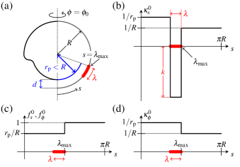
Figure 4: (color online). Setup for numerical calculations, following hohn14 . (a) Geometrical setup: the intrinsic curvature $\kappa_{s}^{0}$ of a spherical shell of undeformed radius $R$ differs from the undeformed curvature in the range $\lambda_{\max}>s>\lambda_{\max}-\lambda$, where $s$ is arclength. Posterior contraction is taken into account by a reduced posterior radius $r_{\mathrm{p}}<R$. These intrinsic curvature and contraction result in deformations that move up the posterior pole by a distance $d$. (b) Corresponding functional form of $\kappa_{s}^{0}$; in the bend region, $\kappa_{s}^{0}=-k<0$. (c) Form of the intrinsic stretches $f_{s}^{0},f_{\phi}^{0}$ for posterior contraction. (d) Functional form of $\kappa_{\phi}^{0}$ for posterior contraction.

III.2 Bifurcation Behaviour

The asymptotic analysis has shown that the coupling of elasticity and geometry constrains small invagination-like deformations both locally and globally, but that contraction can help overcome these global constraints. These ideas carry over to larger deformations of the shell, which must however be studied numerically. For this purpose, we extend the setup of hohn14 , motivated by direct observation of thin sections of fixed embryos: the intrinsic curvature $\kappa_{s}^{0}$ differs from that of undeformed sphere in the range $\lambda_{\max}>s>\lambda_{\max}-\lambda$ of arclength along the shell (Fig. 4a). In this region of length $\lambda$, $\kappa_{s}^{0}=-k$, where $k>0$ (Fig. 4b). This imposed intrinsic curvature results in upward motion of the posterior pole by a distance $d$.

III.2.1 Stability Statements

Our first observation is that, at fixed $\lambda_{\max}$, more than one solution may arise for the same input parameters $(k,\lambda)$. Further understanding is gained by considering, at fixed $\lambda_{\max}$ and for different values of $\lambda$, the relation between $k$ and $d$. The typical behaviour of these branches is plotted in Fig. 5. (The shapes eventually self-intersect; accordingly, these branches end but we expect them to be joined up smoothly to configurations with opposite sides of the shell in contact. The study of such contact configurations typically requires some simplifying assumptions to be made knoche11 , but we do not pursue this further, here.)

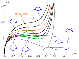
Figure 5: (color online). Bifurcation behaviour of invagination solutions. Solution space for $\lambda_{\max}=1.1R$ and $r_{\mathrm{p}}=R$: each line shows the relation between $k$ and $d$ at some constant $\lambda$. A critical branch (at $\lambda=\lambda_{*}$) separates different types of branches. Branches with $\lambda>\lambda_{\ast}$ feature two extrema; the resulting spinodal curve (thick dashed line) defines a critical point. Insets illustrate representative solution shapes. See text for further explanation.

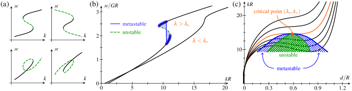
Figure 6: (color online). Stability of invagination solutions. (a) Possible topologies of a double fold in the distinguished $(k,\varkappa)$ bifurcation diagram. Dashed branches are those that the results of maddocks87 imply to be unstable. (b) For $\lambda>\lambda_{\ast}$, S-shaped folds arise in the $(k,\varkappa)$ diagram. From general theory maddocks87 , the middle part of the branch is unstable, while the outer parts are stable. An additional region of metastability is identified by the Maxwell construction. (c) Resulting picture: a region of unstable and metastable solutions expands underneath the critical point.

At the distinguished value $\lambda=\lambda_{\ast}$, a critical branch arises (Fig. 5). It separates two types of branches: first, those with $\lambda<\lambda_{\ast}$, on which $d$ varies mononotonically with $k$, and second, those with $\lambda>\lambda_{\ast}$, where the relation between $d$ and $k$ is more complicated. At large values of $\lambda$, these branches may have a rather involved topology involving loops. At values of $\lambda$ just above $\lambda_{\ast}$, however, there is a range of values of $k$ for which there exist three configurations (Fig. 5). We note that the two outer configurations have $\partial d/\partial k>0$, while the middle one has $\partial d/\partial k<0$. The latter behaviour prefigures instability, which we shall discuss in more detail below. There are thus two points on these branches where $k$, viewed locally as a function of $d$, reaches an extremum. The curve joining up these extrema for different values of $\lambda$ we shall term the ‘spinodal curve’. This curve, in turn, has a maximum at a point on the critical branch, which we shall call the ‘critical point’ and which is characterised by $\lambda_{\ast}$ and the critical curvature, $k_{\ast}$.

The stability of the configurations in Fig. 5 can be assessed by means of general results of bifurcation theory maddocks87 , used recently to discuss the stability of the buckled equilibrium shapes of a pressurised elastic spherical shell knoche11 ; knoche14 . If we let $\varkappa=-\partial\mathcal{E}/\partial k$ denote the conjugate variable to $k$, the key result of maddocks87 is that stability, at fixed $\lambda$, of extremizers of the energy $\mathcal{E}$ can be assessed from the folds in the $(k,\varkappa)$ bifurcation diagram. In particular, stability can only change at folds in the bifurcation diagram. Expanding the bending part of the energy functional (4) for $f_{s}^{0}=f_{\phi}^{0}=1$ and $\kappa_{\phi}^{0}=0$, we find

$$\varkappa=-G\int_{\lambda_{\max}-\lambda}^{\lambda_{\max}}{r_{0}\Bigl{(}f_{s}\kappa_{s}+\nu f_{\phi}\kappa_{\phi}+k\Bigr{)}\,\mathrm{d}s}$$ (35)

with $G=\pi Eh^{3}\big{/}6\bigl{(}1-\nu^{2}\bigr{)}$. (The last term in the integrand is independent of the solution, and may therefore be ignored in what follows.)

The two folds that arise in the $(k,d)$ diagram for $\lambda>\lambda_{\ast}$ (Fig. 5) are compatible a priori with four fold topologies in the $(k,\varkappa)$ diagram (Fig. 6a). However, since a single solution exists for small $k$ (at fixed $\lambda$), the lowest branch must be stable. Further, since the branches do not self-intersect in the $(k,d)$ diagram, they cannot self-intersect in the $(k,\varkappa)$ diagram either. The results of maddocks87 imply that only the first topology in Fig. 6a is compatible with this, and so the fold is S-shaped and traversed upwards in the $(k,\varkappa)$ diagram. It follows in particular that the middle branch, with $\partial d/\partial k<0$ is unstable, and that right branch is stable. (Numerically, one confirms that the branches are indeed S-shaped.) Thus the stability of the branches in this simple bifurcation diagram could also be inferred from the $(k,d)$ diagram (though, in general problems, as discussed in maddocks87 , different bifurcation diagrams may suggest contradictory stability results). However, the Maxwell construction of equal areas landaulifshitzsp can be applied to the $(k,\varkappa)$ diagram (Fig. 6b) to identify metastable solutions beyond the unstable branch. These stability considerations may appear rather technical, but they are in fact very natural: under reflection, the $(d,k)$ diagram maps to the diagram of isotherms of a classical van-der-Waals gas, for which the middle branch is well known to be unstable landaulifshitzsp . Under this analogy, $\mathcal{E}$ corresponds to the Gibbs free energy of the gas.

This analysis cannot immediately be extended to the more exotic topologies that arise for $\lambda$ close to $\lambda_{\max}$ (Fig. 5). We note however that part of these branches must be unstable, too: as above, a single solution exists for small $d$, and so the corresponding branch must be stable. The first fold must be traversed upwards, and the first branch with $\partial d/\partial k<0$ is thus unstable, as above.

An analogous analysis can be carried out for deformations that vary $\lambda$ while keeping $k$ fixed: for $k>k_{\ast}$, the $(d,\lambda)$ diagram is monotonic, but this ceases to be the case for $k<k_{\ast}$. As above, the stability can be inferred from the $(\lambda,d)$ diagram, and the middle branch with $\partial d/\partial\lambda<0$ is unstable, too.

The picture that emerges from this discussion is the following: solutions in a region of parameter space underneath the critical point bounded by the spinodal curve are unstable; a band of solutions on either side of this region and below the critical point are metastable (Fig. 6c), both to perturbations varying $k$ and to perturbations varying $\lambda$. If invagination, driven by a localized region of active bending, is to be stable, it must move around the critical point: if it were to enter the unstable region, the shell would flip back and forth between the ‘shallow’ and ‘deep’ invagination states on either side of the unstable region and suffer large strains in the process. (This makes this kind of instability different from the classical buckling instability of a rod or a ‘popper’ toy pandey : the latter is directed in that, once the instability threshold is crossed, the system will snap to the new preferred configuration and remain there.) The need for a sequence of stable deformations to move around the critical point rationalises the timecourse of invagination in Volvox: initially, a narrow band of cells undergoes cell shape changes, thereby acquiring a high intrinsic curvature. This region of cells then widens, moving around the critical point, whereupon the preferred curvature relaxes and posterior inversion can complete.

III.2.2 Contraction and Criticality

For different values of $\lambda_{\max}$, the critical point traces out a trajectory in parameter space, characterised by $k_{\ast}$ and $\lambda_{\ast}$ (Fig. 7). As $\lambda_{\max}$ increases, $k_{\ast}$ increases, while $\lambda_{\ast}$ decreases. Thus the closer to the equator, the more difficult invagination is, not only because there is less room to fit the posterior into the anterior, but also because a stable invagination requires narrower and narrower invaginations of higher and higher intrinsic curvature.

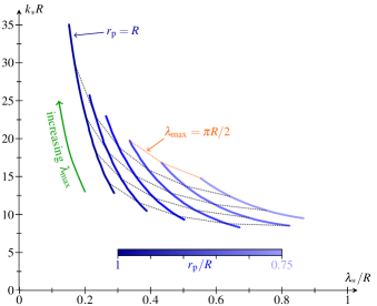
Figure 7: (color online). Contraction and the critical point. Trajectories of critical point in parameter space as $\lambda_{\max}$ is varied, for different values of $r_{\mathrm{p}}$. Thin dotted lines are curves of constant $\lambda_{\max}$. At constant $\lambda_{\max}$, increased contraction leads to decreased $k_{\ast}$ and increased $\lambda_{\ast}$.

We are left to explore how contraction affects the position of the critical point, and hence the invagination. We introduce a reduced posterior radius $r_{\mathrm{p}}<R$ as in hohn14 (Fig. 4a), and modify the intrinsic curvatures and stretches accordingly (Fig. 4b,c,d). Numerically, we observe that, at constant $\lambda_{\max}$, increasing contraction (that is, reducing $r_{\mathrm{p}}$) decreases the critical curvature $k_{\ast}$, and increases $\lambda_{\ast}$ (Fig. 7). Hence contraction aids invagination not only geometrially, but also mechanically: first, it allows invagination close to the equator (which would otherwise be prevented by different parts of the shell touching), and second, it makes stable invagination easier, by reducing $k_{\ast}$. Thus, again, contraction appears as a mechanical means to overcome global geometric constraints.

III.2.3 Asymptotic Analogy

In the asymptotic analysis in the previous section, we restricted ourselves to small deviations of the normal angle from the spherical configuration so that the problem remained analytically tractable. While the leading scaling balances remain the same for large rotations, the resulting non-linear “deep-shell equations” cannot be rescaled so that the dependance on $X$ drops out audolypomeau . Some further insight can, however, be gained in the shallow-shell limit $X\ll 1$: in terms of the inner coordinate $\xi$, we write

$$\beta(\xi)=X\,B(\xi)\ \ \ \ {\rm and}\ \ \ \ \mathit{\Sigma}(\xi)=\varepsilon\,S(\xi).$$ (36)

In the absence of forcing by intrinsic curvature or stretches, the leading-order balance is

$$2S^{\prime\prime}=1-B^{2}\ \ \ \ {\rm and}\ \ \ \ B^{\prime\prime}=SB,$$ (37)

where dashes denote, as before, differentiation with respect to $\xi$.

This balance arises also in the study of a spherical shell pushed by a plane audolypomeau : at large indentations, the shell dimples and the plane remains in contact with it only in a circular transition region joining up the undeformed shell to the isometric dimple. With the matching conditions $B\rightarrow\pm 1$ as $\xi\rightarrow\pm\infty$, (37) describe the leading-order shape of this transition region audolypomeau . Remarkably, this deformation is independent of the contact force, which only arises at the next order in the expansion audolypomeau .

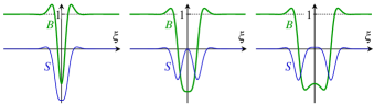
Figure 8: (color online). Examples of “preferred” deformation modes, which are solutions of (37). Of the modes shown, the middle one has the lowest elastic energy.

The appropriate boundary conditions for the invagination case are $B\rightarrow 1$ as $\xi\rightarrow\pm\infty$, and non-constant solutions of (37) can indeed be found numerically (some solutions are shown in Fig. 8). In these modes, the deformations are, in a sense, large compared to intrinsic curvature imposed, making them geometrically ‘preferred’. Their existence lies at the heart of the bifurcation behaviour discussed above.

IV Conclusion

In this paper, we have explored perhaps the simplest intrinsic deformations of a spherical shell: elastic and geometric effects conspire to constrain deformations resulting from a localized region of intrinsic bending. Contraction, a somewhat more global deformation, alleviates these constraints and thereby facilitates the stable transition from one configuration of the shell to another. This rich mechanical behaviour makes a mathematically interesting problem in its own right, yet this analysis has implications for Volvox inversion and wider material design problems.

Experimental studies of Volvox inversion hohn11 ; hohn14 had revealed the existence of posterior contraction, and indeed, the simple elastic model that underlies this paper can only reproduce in vivo shapes once posterior contraction is included hohn14 . Of course, contraction is an obvious means of creating a disparity in the anterior and posterior radii required ultimately to fit one hemisphere into the other, but the present analysis reveals that, beyond this geometric effect, there is another, more mechanical side to the coin: if contraction is present, lower intrinsic curvatures, i.e. less drastic cell shape changes, are required to stably invert the posterior hemisphere. This ascribes a previously unrecognized additional role to these secondary cell shape changes (i.e. those occurring away from the main bend region): just as the shape of the deformed shell arises from a glocal competition between elastic and geometric effects, a combination of local and more global intrinsic properties allow inversion to proceed stably. Thus, as we have pointed out previously, this mechanical analysis rationalises the timecouse of the observed cell shape changes, thereby lending further support to the observation of Höhn et al. hohn14 , that it is a spatio-temporally well regulated sequences of cell shape changes that drives inversion. Thus, the remarkable process of Volvox inversion is mechanically more subtle than it may initially appear to be.

Intrinsic deformations that allow transitions of an elastic object from one configuration to another are of inherent interest in the material design context, and divide into two classes: first, snapping transitions for fast transitions between states, studied in bende , and second, stable sequences of intrinsic deformations. The glocal behaviour of the latter is illustrated by the present analysis: in particular, additional transformations such as contraction can increase the number of stable parameter paths between configurations of the elastic object. In this material design context, non-axisymmetric deformations such as polygonal folds or wrinkles vella11 could also become important, and may warrant a more detailed analysis.

Appendix: Governing Equations

In this appendix, we sketch the derivation of the Euler–Lagrange equations of the energy functional (4), following knoche11 . The variation takes the form

$$\dfrac{\delta\mathcal{E}}{2\pi} =\int_{0}^{\pi R}{r_{0}\Bigl{(}N_{s}\,\delta E_{s}+N_{\phi}\,\delta E_{\phi}\Bigr{)}\;\mathrm{d}s}$$

$$\qquad\qquad+\int_{0}^{\pi R}{r_{0}\Bigl{(}M_{s}\,\delta K_{s}+M_{\phi}\,\delta K_{\phi}\Bigr{)}\;\mathrm{d}s},$$ (A1)

where we have introduced the stresses and moments

$$N_{s} =C\bigl{(}E_{s}+\nu E_{\phi}\bigr{)}, N_{\phi} =C\bigl{(}\nu E_{s}+E_{\phi}\bigr{)},$$ (A2a)

$$M_{s} =D\bigl{(}K_{s}+\nu K_{\phi}\bigr{)}, M_{\phi} =D\bigl{(}\nu K_{s}+K_{\phi}\bigr{)},$$ (A2b)

with $C=Eh\big{/}\bigl{(}1-\nu^{2}\bigr{)}$ and $D=Ch^{2}/12$. (These stresses and moments are expressed here relative to the undeformed configuration.)

The deformed shape of the shell is characterised by the radial and vertical coordinates $r(s)$ and $z(s)$, as well as the angle $\beta(s)$ that the normal to the deformed shell makes with the vertical direction. These geometric quantities obey the equations knoche11

$$\frac{\mathrm{d}r}{\mathrm{d}s}=f_{s}\cos{\beta}, \frac{\mathrm{d}z}{\mathrm{d}s}=f_{s}\sin{\beta}, \frac{\mathrm{d}\beta}{\mathrm{d}s}=f_{s}\kappa_{s}.$$ (A3)

We note that one of these is redundant. The variations $\delta E_{s},\delta E_{\phi},\delta K_{s},\delta K_{\phi}$ are purely geometrical, and one shows that knoche11

$$\delta E_{s} =\sec{\beta}\,\delta r^{\prime}+f_{s}\tan{\beta}\,\delta\beta, \delta E_{\phi} =\dfrac{\delta r}{r_{0}},$$ (A4a)

$$\delta K_{s} =\delta\beta^{\prime}, \delta K_{\phi} =\dfrac{\cos{\beta}}{r_{0}}\delta\beta.$$ (A4b)

The variation (A1) thus becomes

$$\dfrac{\delta\mathcal{E}}{4\pi} =\Bigl{\llbracket}r_{0}N_{s}\sec{\beta}\,\delta r+r_{0}M_{s}\,\delta\beta\Bigr{\rrbracket}-\int_{0}^{\pi R}{\biggl{\{}\frac{\mathrm{d}}{\mathrm{d}s}\Bigl{(}r_{0}N_{s}\sec{\beta}\Bigr{)}-N_{\phi}\biggr{\}}\delta r\;\mathrm{d}s}$$

$$\hskip 170.71652pt+\int_{0}^{\pi R}{\biggl{\{}r_{0}f_{s}N_{s}\tan{\beta}+M_{\phi}\cos{\beta}-\frac{\mathrm{d}}{\mathrm{d}s}\Bigl{(}r_{0}M_{s}\Bigr{)}\biggr{\}}\delta\beta\;\mathrm{d}s},$$ (A5)

upon integration by parts, whence

$$r_{0}f_{s}N_{s}\tan{\beta}+M_{\phi}\cos{\beta}-\frac{\mathrm{d}}{\mathrm{d}s}\Bigl{(}r_{0}M_{s}\Bigr{)}=0,$$ (A6a)

$$\frac{\mathrm{d}}{\mathrm{d}s}\Bigl{(}r_{0}N_{s}\sec{\beta}\Bigr{)}-N_{\phi}=0.$$ (A6b)

These equations, together with two of the geometric relations (A3), describe the shape of the deformed shell. For numerical purposes, it is convenient to remove the singularity at $\beta=\pi/2$ by introducing the transverse shear tension libai ; knoche11 , $Q=-N_{s}\tan{\beta}$, expressed here relative to the undeformed configuration. Force balance arguments libai ; knoche11 show that $Q$ obeys

$$\frac{\mathrm{d}}{\mathrm{d}s}\Bigl{(}r_{0}Q\Bigr{)}+r_{0}f_{s}\kappa_{s}N_{s}+r_{0}f_{\phi}\kappa_{\phi}N_{\phi}=0.$$ (A7)

The solution $Q=-N_{s}\tan{\beta}$ is selected by the boundary condition $Q(0)=0$. At the poles of the shell, the equations have singular terms in them, but these singularities are either removable or the appropriate boundary values are set by symmetry arguments knoche11 . This allows appropriate boundary conditions and values to be derived.

References

- (1) W. Helfrich, Elastic properties of lipid bilayers: Theory and possible experiments, Z. Naturforsch. 28c, 693 (1973).
- (2) J. L. Silverberg, J.-H. Na, A. A. Evans, B. Liu, T. C. Hull, C. D. Santangelo, R. J. Lang, R. C. Hayward, and I. Cohen, Origami structures with a critical transition to bistability arising from hidden degrees of freedom, Nat. Mater. 14, 389 (2015).
- (3) N. P. Bende, A. A. Evans, S. Innes-Gold, L. A. Marin, I. Cohen, R. C. Hayward, and C. D. Santangelo, Geometrically controlled snapping transitions in shells with curved creases, arXiv:1410.7038.
- (4) D. L. Kirk, Volvox: Molecular-Genetic Origins of Multicellularity and Cellular Differentiation (Cambridge University Press, Cambridge, England, 1998).
- (5) A. Weismann, Essays on Heredity and Kindred Biological Problems, (Clarendon Press, Oxord, England, 1892).
- (6) R. E. Goldstein, Green algae as model organisms for biological fluid dynamics, Annu. Rev. Fluid Mech. 47, 343 (2015).
- (7) K. J. Green and D. L. Kirk, Cleavage patterns, cell lineages, and development of a cytoplasmic bridge system in Volvox embryos, J. Cell Biol. 91, 743 (1981).
- (8) K. J. Green, G. L. Viamontes, and D. L. Kirk, Mechanism of formation, ultrastructure, and function of the cytoplasmic bridge system during morphogenesis in Volvox, J. Cell Biol. 91, 756 (1981).
- (9) G. L. Viamontes and D. L. Kirk, Cell shape changes and the mechanism of inversion in Volvox, J. Cell Biol. 75, 719 (1977).
- (10) D. L. Kirk and I. Nishii, Volvox carteri as a model for studying the genetic and cytological control of morpho- genesis, Development, growth and differentiation 43, 621 (2001).
- (11) A. Hallmann, Morphogenesis in the family Volvocaceae: different tactics for turning an embryo right-side out, Protist 157, 445 (2006).
- (12) S. Höhn and A. Hallmann, There is more than one way to turn a spherical cellular monolayer inside out: Type B embryo inversion in Volvox globator, BMC Biol. 9, 89 (2011).
- (13) B. He, K. Doubrovinski, O. Polyakov, and E. Wieschaus, Apical constriction drives tissue-scale hydrodynamic flow to mediate cell elongation, Nature (London) 508, 392 (2014).
- (14) L. A. Lowery and H. Sive, Strategies of vertebrate neuru- lation and a re-evaluation of teleost neural tube formation, Mech. Develop. 121, 1189 (2004).
- (15) M. Eiraku, N. Takata, H. Ishibashi, M. Kawada, E. Sakakura, S. Okuda, K. Sekiguchi, T. Adachi, and Y. Sasai, Self-organizing optic-cup morphogenesis in three- dimensional culture, Nature (London) 472, 51 (2011).
- (16) J. M. Sawyer, J. R. Harrell, G. Shemer, J. Sullivan-Brown, M. Roh-Johnson, and B. Goldstein, Apical constriction: A cell shape change that can drive morphogenesis, Dev. Biol. 341, 5 (2010).
- (17) G. M. Odell, G. Oster, and A. Burnside, The mechanical basis of morphogenesis, Dev. Biol. 85, 446 (1981).
- (18) J. Howard, S. W. Grill, and J. S. Bois, Turing’s next steps: the mechanochemical basis of morphogenesis, Nat. Rev. Mol. Cell Bio. 12, 392 (2011).
- (19) S. Höhn, A. Honerkamp-Smith, P. A. Haas, P. Khuc Trong, and R. E. Goldstein, Dynamics of a Volvox embryo turning itself inside out, Phys. Rev. Lett. 114, 178101 (2015).
- (20) A. Libai and J. G. Simmonds, The Nonlinear Theory of Elastic Shells (Cambridge University Press, Cambridge, England, 2006).
- (21) B. Audoly and Y. Pomeau, Elasticity and Geometry (Oxford University Press, Oxford, England, 2010).
- (22) S. Knoche and J. Kierfeld, Buckling of spherical capsules, Phys. Rev. E 84, 046608 (2011).
- (23) J. H. Maddocks, Stability and Folds, Arch. Rat. Mech. Anal. 99, 301 (1987).
- (24) S. Knoche and J. Kierfeld, Osmotic buckling of spherical capsules, Soft Matter 10, 8358 (2014).
- (25) L. D. Landau and E. M. Lifshitz, Statistical Physics (Butterworth-Heinemann, Oxford, England, 1980).
- (26) A. Pandey, D. E. Moulton, D. Vella, and D. P. Holmes, Dynamics of snapping beams and jumping poppers, Europhys. Lett. 105, 24001 (2014).
- (27) D. Vella, A. Ajdari, A. Vaziei, and A. Boudaoud, Wrinkling of Pressureized Elastic Shells, Phys. Rev. Lett. 107, 174301 (2011).