Dyson–Schwinger approach to Hamiltonian Quantum Chromodynamics

Abstract

The general method for treating non-Gaussian wave functionals in the Hamiltonian formulation of a quantum field theory, which was previously proposed and developed for Yang–Mills theory in Coulomb gauge, is generalized to full QCD. For this purpose the quark part of the QCD vacuum wave functional is expressed in the basis of coherent fermion states, which are defined in term of Grassmann variables. Our variational ansatz for the QCD vacuum wave functional is assumed to be given by exponentials of polynomials in the occurring fields and, furthermore, contains an explicit coupling of the quarks to the gluons. Exploiting Dyson–Schwinger equation techniques, we express the various $n$-point functions, which are required for the expectation values of observables like the Hamiltonian, in terms of the variational kernels of our trial ansatz. Finally the equations of motion for these variational kernels are derived by minimizing the energy density.

I Introduction

One of the major challenges of theoretical particle physics is the understanding of the low-energy sector of Quantum Chromodynamics (QCD). Despite many years of intensive research, a thorough and unified picture of the low-energy phenomena of strong interactions, i.e., confinement and spontaneous breaking of chiral symmetry, is still lacking. Much insight has been gained by means of lattice Monte-Carlo calculations, in particular on the gluon sector of QCD. However, despite much progress, the treatment of dynamical chiral quarks is still a challenge for the lattice approach, which furthermore struggles to describe the phase diagram of QCD at finite baryon density due to the notorious sign problem. In addition and in general, a thorough understanding of physical phenomena cannot be achieved by numerical lattice simulations alone but analytic methods, albeit approximate ones, are needed as well.

Over the last decade substantial efforts have been undertaken to develop non-perturbative continuum approaches to QCD. These approaches are based on functional methods and can be roughly divided into three classes: i) Dyson–Schwinger equations (DSEs) in Landau Alkofer:2000wg ; *Fischer:2006ub; Fischer:2008uz ; Binosi:2009qm and Coulomb gauges Zwanziger:1998ez ; Watson:2006yq ; Watson:2007mz ; *Watson:2007vc; *Popovici:2008ty; Reinhardt:2008pr ; Watson:2008fb ; *Watson:2010cn; *Watson:2011kv; *Watson:2012ht; Popovici:2010mb ; *Popovici:2010ph; *Popovici:2011yz, ii) functional renormalization group (FRG) flow equations Pawlowski:2005xe ; Gies:2006wv ; Braun:2011pp and iii) the variational approach to Hamiltonian QCD Schutte:1985sd ; *Szczepaniak:2001rg; Feuchter:2004mk ; *Reinhardt:2004mm. These three approaches are intimately related. The first two approaches are based on the functional integral formulation of QCD in either Landau or Coulomb gauge, while the variational approach has been mainly applied to the Hamiltonian formulation in Coulomb gauge but has been recently also extended to the effective action of the functional integral formulation in Landau gauge Quandt:2013wna ; *Quandt:2015aaa. The equations of motion of the first two approaches are in fact very similar and in a certain approximation (replacing the renormalization group scale $k$ in the loop integrals by its infrared value $k=0$) the FRG flow equation becomes a Dyson–Schwinger equation. The FRG flow equations have been also applied to the Hamiltonian approach in Coulomb gauge and results similar to those in the variational treatment were found Leder:2010ji ; Leder:2011yc . Furthermore, the DSE techniques can be very advantageously exploited to carry out the variational approach with non-Gaussian wave functionals describing interacting quantum fields Campagnari:2010wc . In the present paper we use the Dyson–Schwinger equations to develop a variational approach to the Hamiltonian formulation of QCD.

Previous variational studies within the Hamiltonian approach have focused on the Yang–Mills sector and used Gaussian-type ansätze for the vacuum wave functional. This has provided a decent description of both the infrared (IR) and ultraviolet (UV) sector in rough agreement with the existing lattice data. In particular, a linearly rising static quark potential Epple:2006hv ; Pak:2009em and a perimeter law Reinhardt:2007wh for the ’t Hooft loop tHooft:1977hy were found, which are both features of the confined phase. Also the connection to the dual Meissner effect (an appealing picture of confinement) was established Reinhardt:2008ek . More recently, the deconfinement phase transition was studied at finite temperatures Reinhardt:2011hq ; Heffner:2012sx and the effective potential of the Polyakov loop was calculated Reinhardt:2012qe ; Reinhardt:2013iia . The obtained critical temperature is in reasonable agreement with the lattice data. Furthermore, the order of the phase transition was correctly reproduced Reinhardt:2013iia . In the zero-temperature calculation the obtained static gluon propagator agrees with the lattice data in the IR and UV but misses some strength in the mid-momentum regime. This missing strength can be attributed to the absence of non-Gaussian terms in the vacuum wave functional Campagnari:2010wc .

Generally, Gaussian wave functionals describe quantum field theories in the independent (quasi-)particle approximation, while truly interacting quantum fields possess non-Gaussian vacuum wave functionals. In Ref. Campagnari:2010wc a general method for treating non-Gaussian trial wave functionals in a quantum field theory was proposed. This method relies on Dyson–Schwinger-type of equations to express the various $n$-point functions of the quantum field in terms of the variational kernels contained in the exponent of the ansatz for the vacuum wave functional. So far this method has been formulated for Bose fields only and was applied to the Yang–Mills sector of QCD using a wave functional which includes, besides the usual quadratic term of the Gaussian, also cubic and quartic terms of the gauge field. In principle, the approach put forward in Ref. Campagnari:2010wc is general enough to deal with any interacting quantum field theory. In the present paper we extend this approach to full QCD. The central point will be the treatment of fermion fields interacting with Bose (gauge) fields. To exploit the Dyson–Schwinger equation techniques, the second quantization of the fermion sector of the theory has to be formulated in terms of Grassmann variables. For this purpose we express the quark part of the QCD vacuum wave functional in terms of coherent fermion states. We will formulate the present approach to Hamiltonian QCD for general wave functionals but work out the Dyson–Schwinger-type of equations only for those wave functionals whose exponent is bilinear in the quark field.

The QCD vacuum wave functional is chosen as the exponential of some polynomial functional of the quark and gluon fields. The coefficient functions of the various polynomial terms are treated as variational kernels. By means of Dyson–Schwinger equation techniques we express the various $n$-point functions, needed for the vacuum expectation value of observables like the Hamiltonian, in terms of these variational kernels, which in this context figure as bare vertices. The resulting equations are different from the usual DSEs, which relate the various full (dressed) propagators and vertices to the bare (inverse) propagators and vertices occurring in the classical action, and are termed canonical recursive DSEs (CRDSEs) in the following. By means of the CRDSEs we express the vacuum expectation value of the QCD-Hamiltonian as functional of the variational kernels of our vacuum wave functional. Minimization of the energy density with respect to these variational kernels results then in a set of equations of motion (referred to as ‘gap equations’), which have to be solved together with the CRDSEs.

The organization of the rest of the paper is as follows: In Sec. II we briefly summarize the basic ingredients of the formulation of the second quantization in terms of Grassmann variables and present the quark part of the QCD wave functional in the basis of coherent fermion states. In Sec. III we derive the general form of the CRDSEs for the static Green functions of QCD, assuming a QCD vacuum wave functional which in particular contains the coupling between quarks and gluons. In Sec. IV, after introducing the QCD Hamilton operator in Coulomb gauge, we calculate the energy density in the vacuum state. The variational principle is carried out in Sect. V, where we derive the equations of motion for the variational kernels of our QCD vacuum wave functional. A short summary and our conclusions are given in Sect. VI. Here we also briefly discuss further applications of the approach developed in this work.

II Coherent State Description of the Fermionic Fock Space

As demonstrated in Ref. Campagnari:2010wc for Yang–Mills theory, the use of non-Gaussian wave functionals in the Hamiltonian approach can be conveniently accomplished by exploiting Dyson–Schwinger equation techniques known from the Lagrangian (functional integral) formulation of quantum field theory. This refers, in particular, to wave functionals describing interacting fields. To exploit the DSE techniques in the Hamiltonian formulation of QCD it is necessary to represent the quark operators and wave functionals in terms of anti-commuting Grassmann fields. In this representation the matrix elements between Fock-space states are then given by functional integrals over Grassmann fields. The formulation of the second quantization in terms of Grassmann variables becomes particularly efficient when coherent fermion states are used. Below we will briefly review the basic ingredients of the coherent fermion state representation of Fock space and apply it to Dirac fermions.

II.1 Coherent Fermion States and Grassmann Variables

Consider a Fermi system described in second quantization in terms of creation and annihilation operators $b^{\dagger}_{k}$, $b_{k}$, satisfying the usual anti-commutation relations

$$\mathopen{\big{\{}}b_{k},b_{l}\mathclose{\big{\}}}=0=\mathopen{\big{\{}}b^{\dagger}_{k},b^{\dagger}_{l}\mathclose{\big{\}}},\qquad\mathopen{\big{\{}}b_{k},b^{\dagger}_{l}\mathclose{\big{\}}}=\delta_{kl},$$

where the subscripts $k$, $l$, … denote a complete set of single-particle states. Let $\lvert 0\rangle$ be the Fock vacuum, i.e.

$$b_{k}\lvert 0\rangle=0.$$

The coherent fermion states $\lvert\zeta\rangle$ are defined as eigenstates of the annihilation operators Reinhardt:qm2

$$b_{k}\lvert\zeta\rangle=\zeta_{k}\lvert\zeta\rangle,$$ (1)

where the $\zeta_{k}$ are anti-commuting (Grassmann) variables $\mathopen{\big{\{}}\zeta_{k},\zeta_{l}\mathclose{\big{\}}}=0$. The corresponding bra-vectors are defined as left eigenstates of the creation operators

$$\langle\zeta\rvert b^{\dagger}_{k}=\langle\zeta\rvert\zeta^{*}_{k}\,,$$ (2)

where the operation ‘$*$’ denotes the involution. We will keep the same symbol ‘$*$’ also for the usual complex conjugation of ordinary complex numbers.

The coherent fermion states defined by Eqs. (1) and (2) can be expressed in Fock space as

$$\lvert\zeta\rangle=\exp(\zeta\cdot b^{\dagger})\lvert 0\rangle,\quad\quad\langle\zeta\rvert=\langle 0\rvert\exp(b\cdot\zeta^{*}).$$ (3)

Here we have skipped the indices and used the short-hand notation

$$\eta^{*}\cdot\zeta=\sum_{k}\eta^{*}_{k}\zeta_{k}.$$

From the representation Eq. (3) one easily finds for the scalar product of two coherent states

$$\langle\eta|\zeta\rangle=\mathop{}\!\mathrm{e}^{\eta^{*}\cdot\zeta}.$$

The coherent fermion states form an over-complete basis of the Fock space, in which the unit operator has the representation

$$\mathbbm{1}=\int\mathop{}\!{\mathrm{d}}\zeta^{*}\mathop{}\!{\mathrm{d}}\zeta\>\mathop{}\!\mathrm{e}^{-\zeta^{*}\cdot\zeta}\lvert\zeta\rangle\langle\zeta\rvert,\qquad\text{with }\mathop{}\!{\mathrm{d}}\zeta^{*}\mathop{}\!{\mathrm{d}}\zeta\equiv\prod_{k}\mathop{}\!{\mathrm{d}}\zeta^{*}_{k}\mathop{}\!{\mathrm{d}}\zeta_{k}\,.$$ (4)

An arbitrary state $\lvert\varPhi\rangle$ of the Fock space can be expressed in the basis of coherent fermion states $\lvert\zeta\rangle$ by taking the scalar product

$$\varPhi(\zeta^{*})=\langle\zeta|\varPhi\rangle,$$ (5)

which can be interpreted as the “coordinate representation” of fermion states with the Grassmann variables interpreted as classical fermion coordinates. From the representation Eq. (3) it is clear that the $\varPhi(\zeta^{*})$ are functionals of the $\zeta^{*}_{k}$, which can be Taylor expanded

$$\varPhi(\zeta^{*})=\sum_{n}\sum_{k_{1}\dots k_{n}}\varPhi_{k_{1}\dots k_{n}}\zeta^{*}_{k_{1}}\dots\zeta^{*}_{k_{n}}\,,$$ (6)

where the $\varPhi_{k_{1}\dots k_{n}}$ are complex numbers. The representation of bra vectors is obtained by taking the adjoint of Eq. (5)

$$\langle\varPhi|\zeta\rangle=\bigl{(}\varPhi(\zeta^{*})\bigr{)}^{*}\equiv\varPhi^{*}(\zeta)$$ (7)

and is obviously a function of the variables $\zeta_{k}$. From Eq. (6) we find

$$\varPhi^{*}(\zeta)=\sum_{n}\sum_{k_{1}\dots k_{n}}\varPhi^{*}_{k_{1}\dots k_{n}}\zeta_{k_{n}}\dots\zeta_{k_{1}}.$$

The Fock-space states are given by functions of the creation operators $f(b^{\dagger})$ acting on the vacuum state

$$\lvert\varPhi\rangle=f(b^{\dagger})\lvert 0\rangle.$$

From Eq. (2) we find then the corresponding coherent state representation

$$\varPhi(\zeta^{*})=f(\zeta^{*}),$$

where we have used $\langle\zeta|0\rangle=1$, which follows immediately from Eq. (3). The scalar product between two Fock states $|\varPhi\rangle$ and $|\varPsi\rangle$ is easily obtained in the basis of coherent states by inserting the completeness relation Eq. (4)

$$\langle\varPsi|\varPhi\rangle=\int\mathop{}\!{\mathrm{d}}\zeta^{*}\mathop{}\!{\mathrm{d}}\zeta\>\mathop{}\!\mathrm{e}^{-\zeta^{*}\cdot\zeta}\,\varPsi^{*}(\zeta)\,\varPhi(\zeta^{*}),$$ (8)

where we have also used the definitions (5) and (7). Using Eq. (2) and

$$\langle\zeta\rvert b_{k}=\frac{\partial}{\partial\zeta^{*}_{k}}\>\langle\zeta\rvert$$

we find for the action of an operator on a Fock state in the coherent state basis

$$\langle\zeta\rvert O(b,b^{\dagger})\lvert\varPhi\rangle=O\bigl{(}\tfrac{\partial}{\partial\zeta^{*}},\zeta^{*}\bigr{)}\,\varPhi(\zeta^{*})$$

and similarly for matrix elements between states of Fock space

$$\langle\varPsi\rvert O(b,b^{\dagger})\lvert\varPhi\rangle=\int\mathop{}\!{\mathrm{d}}\zeta^{*}\mathop{}\!{\mathrm{d}}\zeta\>\mathop{}\!\mathrm{e}^{-\zeta^{*}\cdot\zeta}\,\varPsi^{*}(\zeta)\,O\bigl{(}\tfrac{\partial}{\partial\zeta^{*}},\zeta^{*}\bigr{)}\,\varPhi(\zeta^{*}).$$ (9)

In the next subsection the coherent fermion state representation of the Fermionic Fock space given above is extended to Dirac Fermions.

II.2 Coherent-State Representation of Dirac Fermions

The description of Fermi systems in terms of Grassmann variables outlined above can be immediately applied to Dirac fermions once the fermion field is expressed in terms of creation and annihilation operators.

In this paper we use a compact notation in which a single digit 1, 2, … represents all indices of the time-independent field. For example, for the quark field we have

$$\psi(1)\equiv\psi_{s_{1}}^{k_{1}}(\vx_{1}),$$

where $s_{1}$ denotes the Dirac spinor index, while $k_{1}$ stands for the colour (and possibly flavour) index. A repeated index implies integration of spatial coordinates and summation over the discrete indices (spinor, colour, flavour). Furthermore, we define the Kronecker symbol in the numerical indices to contain besides the usual Kronecker symbol for the discrete indices also the $\delta$ function for the continuous coordinates, e.g.

$$\delta(1,2)=\delta(\vx_{1}-\vx_{2})\,\delta_{s_{1}s_{2}}\delta^{k_{1}k_{2}}\dots$$

The usual anticommutation relation for the Dirac field reads

$$\mathopen{\big{\{}}\psi(1),\psi^{\dagger}(2)\mathclose{\big{\}}}=\delta(1,2).$$ (10)

Let

$$h_{0}(1,2)=\delta^{m_{1}m_{2}}\bigl{(}-\mathrm{i}\mkern 1.0mu\bm{\mathrm{\alpha}}\cdot\grad+\beta m\bigr{)}\delta(\vx_{1}-\vx_{2})$$ (11)

denote the Dirac Hamiltonian of free quarks with a bare mass $m$. This Hamiltonian possesses (an equal number of) positive and negative energy eigenstates. We can expand the quark field $\psi(1)$ in terms of these eigenstates. Let $\psi_{\pm}(1)$ denote the part formed from the positive/negative energy modes. Obviously, we have

$$\psi(1)=\psi_{+}(1)+\psi_{-}(1).$$

For the subsequent considerations it will be convenient to introduce orthogonal projectors $\Lambda_{\pm}$ onto the positive and negative energy part of the Dirac field, i.e.

$$\psi_{\pm}(1)=\Lambda_{\pm}(1,2)\psi(2),$$ (12)

satisfying

$$\Lambda_{+}(1,2)+\Lambda_{-}(1,2)=\delta(1,2),\qquad\Lambda_{+}(1,2)\Lambda_{-}(2,3)=0,\qquad\Lambda_{\pm}(1,2)\,\Lambda_{\pm}(2,3)=\Lambda_{\pm}(1,3).$$ (13)

These projectors can be expressed by spectral sums over the positive and negative, respectively, energy modes of the Hermitian Dirac Hamiltonian $h_{0}(1,2)$, and satisfy $\Lambda_{\pm}^{\dagger}(1,2)=\Lambda_{\pm}(1,2)$. With this relation we find for the adjoint fermion operator from Eq. (12)

$$\psi_{\pm}^{\dagger}(1)=\psi^{\dagger}(2)\Lambda_{\pm}(2,1).$$ (14)

From Eqs. (12) and (14) it follows with (13)

$$\mathopen{\big{\{}}\psi_{\pm}(1),\psi_{\pm}^{\dagger}(2)\mathclose{\big{\}}}=\Lambda_{\pm}(1,2),\qquad\mathopen{\big{\{}}\psi_{\pm}(1),\psi_{\mp}^{\dagger}(2)\mathclose{\big{\}}}=0.$$

In the bare (free Dirac) vacuum state $\lvert 0\rangle$ all negative energy modes are filled, while the positive energy modes are empty, implying

$$\psi_{+}(1)\lvert 0\rangle=0=\psi_{-}^{\dagger}(1)\lvert 0\rangle.$$ (15)

In analogy to Eq. (1) we define coherent fermion states $\lvert\xi\rangle\equiv\lvert\xi_{+},\xi_{-}\rangle$ by

$$\psi_{+}(1)\lvert\xi\rangle=\xi_{+}(1)\lvert\xi\rangle,\qquad\psi_{-}^{\dagger}(1)\lvert\xi\rangle=\xi_{-}^{\dagger}(1)\lvert\xi\rangle,$$ (16)

where $\xi_{\pm}$ are Grassmann fields. Since $\psi_{\pm}(1)=\Lambda_{\pm}(1,2)\psi_{\pm}(2)$, the Grassmann fields also satisfy

$$\xi_{\pm}(1)=\Lambda_{\pm}(1,2)\xi_{\pm}(2)$$

and the positive- and negative-energy component fields can be assembled into a single Grassmann-valued spinor field

$$\xi(1)=\xi_{+}(1)+\xi_{-}(1),\qquad\xi_{\pm}(1)=\Lambda_{\pm}(1,2)\xi(2)$$ (17)

satisfying

$$\frac{\delta\xi_{\pm}(1)}{\delta\xi_{\pm}(2)}=\Lambda_{\pm}(1,2),\qquad\frac{\delta\xi^{\dagger}_{\pm}(1)}{\delta\xi^{\dagger}_{\pm}(2)}=\Lambda_{\pm}(2,1).$$ (18)

The coherent fermion states defined by Eq. (16) have the Fock-space representation [cf. Eq. (3)]

$$\lvert\xi\rangle=\exp\mathopen{}\mathclose{{}\left[\xi_{+}(1)\psi^{\dagger}_{+}(1)+\xi_{-}^{\dagger}(1)\psi_{-}(1)}\right]\lvert 0\rangle$$

from which follows

$$\psi^{\dagger}_{+}(1)\lvert\xi\rangle=\frac{\delta}{\delta\xi_{+}(1)}\lvert\xi\rangle,\qquad\psi_{-}(1)\lvert\xi\rangle=\frac{\delta}{\delta\xi_{-}^{\dagger}(1)}\lvert\xi\rangle.$$ (19)

Using Eqs. (16) and (19) the action of Dirac field operators on fermion states $\lvert\varPhi\rangle$ is expressed in the basis of coherent states as

$$\begin{split}\langle\xi\rvert\psi(1)\lvert\varPhi\rangle&=\mathopen{}\mathclose{{}\left(\xi_{-}(1)+\frac{\delta}{\delta\xi_{+}^{\dagger}(1)}}\right)\varPhi[\xi_{+}^{\dagger},\xi_{-}],\\ \langle\xi\rvert\psi^{\dagger}(1)\lvert\varPhi\rangle&=\mathopen{}\mathclose{{}\left(\xi_{+}^{\dagger}(1)+\frac{\delta}{\delta\xi_{-}(1)}}\right)\varPhi[\xi_{+}^{\dagger},\xi_{-}],\end{split}$$ (20)

where $\langle\xi|\Phi\rangle\equiv\varPhi[\xi_{+}^{\dagger},\xi_{-}]$ is the coherent-state representation of the quark vacuum wave functional $\lvert\varPhi\rangle$, which can be interpreted as the “coordinate representation” of the latter. Notice that from the definition Eq. (16) of the coherent fermion states follows that the quark vacuum wave functional depends only on $\xi_{+}^{\dagger}$ and $\xi_{-}$.

In analogy to Eq. (9) the matrix element of an operator $\mathcal{O}$ between fermionic Fock states $|\varPhi_{1}\rangle$ and $|\varPhi_{2}\rangle$ is given by

$$\langle\varPhi_{1}\rvert\mathcal{O}[\psi,\psi^{\dagger}]\lvert\varPhi_{2}\rangle=\int\mathcal{D}\xi^{\dagger}\,\mathcal{D}\xi\>\mathop{}\!\mathrm{e}^{-\mu}\>\varPhi_{1}^{*}[\xi_{+},\xi_{-}^{\dagger}]\>\mathcal{O}\bigl{[}\xi_{-}+\tfrac{\delta}{\delta\xi_{+}^{\dagger}},\xi_{+}^{\dagger}+\tfrac{\delta}{\delta\xi_{-}}\bigr{]}\>\varPhi_{2}[\xi_{+}^{\dagger},\xi_{-}],$$ (21)

where we have introduced the quantity

$$\mu=\xi^{\dagger}_{+}(1)\,\xi_{+}(1)-\xi^{\dagger}_{-}(1)\,\xi_{-}(1),$$ (22)

arising from the integration measure of the Grassmann fields [cf. Eq. (8)]. Note that $\mu$, being bilinear in the Grassmann variables, commutes with any element of the Grassmann algebra. This quantity can be rewritten with the help of Eqs. (13) and (17) as

$$\mu=\xi^{\dagger}(1)\bigl{[}\Lambda_{+}(1,2)-\Lambda_{-}(1,2)\bigr{]}\xi(2)\equiv\xi^{\dagger}(1)\,Q_{0}^{-1}(1,2)\,\xi(2),$$ (23)

where the quantity

$$Q_{0}^{-1}(1,2)=\Lambda_{+}(1,2)-\Lambda_{-}(1,2)=Q_{0}(1,2)$$ (24)

represents the free static quark propagator

$$Q_{0}(1,2)=\langle 0\rvert\mathopen{\big{[}}\psi(1),\psi^{\dagger}(2)\mathclose{\big{]}}\lvert 0\rangle,$$ (25)

with $\lvert 0\rangle$ being the Fock vacuum Eq. (15) of the free quarks, as we will discuss in more detail at the end of Sec. III.3.

II.3 Coordinate Representation of QCD Wave Functionals

With the coherent states $\lvert\xi\rangle$ [Eq. (16)] of the Dirac fermions at hand we are now in a position to express QCD wave functionals in the coordinate representation. The coordinates of the gauge field are its spatial components $A_{i}^{a}(\vx)$. In analogy to the fermion field we will collect all indices of the gluon field in a single digit $A(1)\equiv A_{i_{1}}^{a_{1}}(\vx_{1})$, where $a_{1}$ denotes the colour index of the adjoint representation and $i_{1}$ is a spatial Lorentz index. In the coordinate representation of the wave functional of the Yang–Mills sector $\varPsi[A]=\langle A|\varPsi\rangle$ we have for the operators of the canonical variables

$$\langle A\rvert\hat{A}(1)\lvert\varPsi\rangle=A(1)\,\varPsi[A],\qquad\langle A\rvert\hat{\Pi}(1)\lvert\varPsi\rangle=\frac{\delta\varPsi[A]}{\mathrm{i}\,\delta A(1)}.$$

We will work here in Coulomb gauge $\partial_{i}A_{i}^{a}=0$, where only the transverse components of the gauge field are left. In our compact notation we have

$$\frac{\delta A(1)}{\delta A(2)}=t(1,2),$$ (26)

where

$$t(1,2)=\delta^{a_{1}a_{2}}\mathopen{}\mathclose{{}\left(\delta_{i_{1}i_{2}}-\frac{\partial_{i_{1}}\partial_{i_{2}}}{\partial^{2}}}\right)\delta(\vx_{1}-\vx_{2})$$

is the transverse projector.

The vacuum state of QCD can be written in the coordinate representation (i.e., coherent-state representation for the fermions) as

$$\varPsi[A,\xi^{\dagger}_{+},\xi_{-}]\eqcolon\exp\mathopen{}\mathclose{{}\left\{-\frac{1}{2}\,S_{A}[A]-S_{f}[\xi^{\dagger}_{+},\xi_{-},A]}\right\},$$ (27)

where $S_{A}$ defines the vacuum wave functional of pure Yang–Mills theory, while $S_{f}$ defines the wave functional of the fermions interacting with the gluons. On general grounds $S_{f}$ contains only even powers of Grassmann variables so that this quantity, as well as the vacuum wave functional $\varPsi[A,\xi^{\dagger}_{+},\xi_{-}]$, commutes with any Grassmann field.

A comment is here in order concerning the representation Eq. (27) of the vacuum wave functional for the gluon and quark fields. For the bosonic gluon field we use here the usual “coordinate” representation regarding its spatial components as the (classical) coordinates of the theory. As already discussed in Sec. II.1, the classical analogues of the fermion fields are the Grassmann variables and the “coordinate representation” of the fermion wave functional is the coherent (-fermion) state representation, Eq. (5). We could also use bosonic coherent states for the gluons but this is not necessary and we will not use it since the usual coordinate representation is in this case quite convenient.

For sake of illustration we quote the expressions for the perturbative QCD vacuum state Campagnari:2009km ; *Campagnari:2009wj; *Campagnari:2014hda. The perturbative Yang–Mills vacuum is obtained by choosing in Eq. (27) the quadratic gluonic “action”

$$S_{A}=\int\frac{\mathrm{d}^{3}p}{(2\pi)^{3}}\>A_{i}^{a}(\vp)\,\lvert\vp\rvert\,A_{i}^{a}(-\vp).$$ (28)

On the other hand, the ground state $\lvert 0\rangle$ [Eq. (15)] of the free (perturbative) quarks reads in the coherent state basis $\varPhi[\xi_{+}^{\dagger},\xi_{-}]=\langle\xi|0\rangle=1$ (i.e., $S_{f}[\xi_{+}^{\dagger},\xi_{-},A]=0$). This is because the kinematics of the free fermions is already encoded in the integration measure $\mu$ of the Grassmann fields, see Eqs. (21)–(23).

Eventually we are interested in the Hamiltonian formulation of QCD in Coulomb gauge. The coordinate representation of gluonic states and matrix elements has been presented in Ref. Campagnari:2010wc . Writing the QCD vacuum wave functional in the form (27) and using the representation (21) of the fermionic matrix elements, expectation values in gauge-fixed QCD are given by

$$\mathopen{}\mathclose{{}\left\langle\mathcal{O}[\psi,\psi^{\dagger},A,\Pi]}\right\rangle=\int\mathcal{D}\xi^{\dagger}\,\mathcal{D}\xi\,\mathcal{D}A\>\mathcal{J}_{A}\mathop{}\!\mathrm{e}^{-\mu}\,\mathop{}\!\mathrm{e}^{-\frac{1}{2}S_{A}-S_{f}^{*}}\>\mathcal{O}\bigl{[}\xi_{-}+\tfrac{\delta}{\delta\xi_{+}^{\dagger}},\,\xi_{+}^{\dagger}+\tfrac{\delta}{\delta\xi_{-}},\,A,\,\tfrac{\delta}{\mathrm{i}\mkern 1.0mu\delta A}\bigr{]}\>\mathop{}\!\mathrm{e}^{-\frac{1}{2}S_{A}-S_{f}},$$ (29)

where

$$\mathcal{J}_{A}=\operatorname{Det}G_{A}^{-1}$$ (30)

is the Faddeev–Popov determinant. In Coulomb gauge the Faddeev–Popov operator reads

$$G^{-1}_{A}=\bigl{(}-\delta^{ab}\,{\partial^{2}_{\vx}}-g\,f^{acb}A^{c}_{i}(\vx)\,\partial_{i}^{\vx}\bigr{)}\delta(\vx-\vy)\,.$$ (31)

Here $g$ is the bare coupling constant and $f^{acb}$ are the structure constants of the $\mathfrak{su}(N)$ algebra. The functional integration in Eq. (29) runs over transverse gauge field configurations and is, in principle, restricted to the first Gribov region or, more precisely, to the fundamental modular region.

Once the functional derivatives in Eq. (29) are taken, the vacuum expectation value of an operator boils down to a functional average of the form

$$\langle f[A,\xi,\xi^{\dagger}]\rangle=\int\mathcal{D}\xi^{\dagger}\,\mathcal{D}\xi\,\mathcal{D}A\>\mathcal{J}_{A}\>\mathop{}\!\mathrm{e}^{-S_{A}-S_{f}-S_{f}^{*}-\mu}\>f[A,\xi,\xi^{\dagger}],$$ (32)

where $f$ is a functional of the fields only (i.e., $f$ contains no functional derivatives).

For the variational approach to QCD to be developed later we need the vacuum expectation values of products of gluon operators $A$, $\Pi$, and, in particular, quark field operators $\psi$, $\psi^{\dagger}$. Furthermore, to exploit DSEs techniques we have to express these expectation values by $n$-point functions of the Grassmann fields $\xi$, $\xi^{\dagger}$. This can be achieved by means of Eq. (20). To illustrate how this is accomplished we consider temporarily the quark sector only and omit the integration over the gauge field. Using Eqs. (21) and (27) we obtain for the quark bilinear

$$\langle\psi(1)\,\psi^{\dagger}(2)\rangle=\int{\cal{D}}\xi^{\dagger}{\cal{D}}\xi\>\mathop{}\!\mathrm{e}^{-\mu-S_{f}^{*}}\biggl{(}\xi_{-}(1)+\frac{\delta}{\delta\xi^{\dagger}_{+}(1)}\biggr{)}\biggl{(}\xi_{+}^{\dagger}(2)+\frac{\delta}{\delta\xi_{-}(2)}\biggr{)}\mathop{}\!\mathrm{e}^{-S_{f}}.$$

Since $S_{f}^{*}$ is independent of $\xi_{+}^{\dagger}$ and $\xi_{-}$ it is convenient to perform integrations by parts with respect to $\xi^{\dagger}_{+}(1)$ and $\xi_{-}(2)$. The integration by parts with respect to $\xi_{+}^{\dagger}(1)$ yields

$$\langle\psi(1)\,\psi^{\dagger}(2)\rangle=\int{\cal{D}}\xi^{\dagger}{\cal{D}}\xi\>\mathop{}\!\mathrm{e}^{-\mu-S_{f}^{*}}\>\xi(1)\mathopen{}\mathclose{{}\left(\xi_{+}^{\dagger}(2)+\frac{\delta}{\delta\xi_{-}(2)}}\right)\mathop{}\!\mathrm{e}^{-S_{f}},$$

where we have used the first equation of Eq. (17). In the same way an integration by parts with respect to $\xi_{-}(2)$ yields

$$\langle\psi(1)\,\psi^{\dagger}(2)\rangle =\int{\cal{D}}\xi^{\dagger}{\cal{D}}\xi\>\mathop{}\!\mathrm{e}^{-S_{f}^{*}-\mu}\mathopen{}\mathclose{{}\left(\xi(1)\,\xi_{+}^{\dagger}(2)+\frac{\delta\xi(1)}{\delta\xi_{-}(2)}+\xi(1)\>\frac{\delta\mu}{\delta\xi_{-}(2)}}\right)\mathop{}\!\mathrm{e}^{-S_{f}}$$

$$=\int{\cal{D}}\xi^{\dagger}{\cal{D}}\xi\>\mathop{}\!\mathrm{e}^{-S_{f}^{*}-\mu}\>\xi(1)\,\xi^{\dagger}(2)\,\mathop{}\!\mathrm{e}^{-S_{f}}+\Lambda_{-}(1,2),$$ (33)

where again Eqs. (17) and (18) and the normalization of the functional integral were used. Finally, we can generalize Eq. (33) to the vacuum expectation value of full QCD (i.e., taking also the functional average over the gluon sector) and include also a functional $f[A]$ of the gauge field. One obtains then

$$\langle\psi(1)\,\psi^{\dagger}(2)\,f[A]\rangle=\langle\xi(1)\,\xi^{\dagger}(2)\,f[A]\rangle+\Lambda_{-}(1,2)\langle f[A]\rangle.$$ (34)

Using the anticommutation relation Eq. (10), from the last relation follows

$$\langle\psi^{\dagger}(1)\,\psi(2)\,f[A]\rangle=\langle\xi^{\dagger}(1)\,\xi(2)\,f[A]\rangle+\Lambda_{+}(2,1)\langle f[A]\rangle.$$ (35)

The expectation value of four fermion operators can be derived along the same lines, resulting in

$$\begin{split}\langle\psi^{\dagger}(1)\,\psi(2)\,\psi^{\dagger}(3)\,\psi(4)\,f[A]\rangle={}&\langle\xi^{\dagger}(1)\,\xi(2)\,\xi^{\dagger}(3)\,\xi(4)\,f[A]\rangle+\\ &+\langle\xi^{\dagger}(1)\,\xi(2)\,f[A]\rangle\,\Lambda_{+}(4,3)+\langle\xi(2)\,\xi^{\dagger}(3)\,f[A]\rangle\,\Lambda_{+}(4,1)\\ &+\langle\xi^{\dagger}(3)\,\xi(4)\,f[A]\rangle\,\Lambda_{+}(2,1)+\langle\xi^{\dagger}(1)\,\xi(4)\,f[A]\rangle\,\Lambda_{-}(2,3)\\ &+\bigl{[}\Lambda_{+}(2,1)\,\Lambda_{+}(4,3)+\Lambda_{+}(4,1)\,\Lambda_{-}(2,3)\bigr{]}\langle f[A]\rangle.\end{split}$$ (36)

III Canonical Recursive Dyson–Schwinger Equations of QCD

As already discussed in the introduction, in the Hamiltonian approach to a quantum field theory the use of non-Gaussian wave functionals is most conveniently accomplished by exploiting DSE techniques known from the functional integral approach. In the Hamiltonian approach, the scalar products or matrix elements between the wave functionals are given by functional integrals [see Eq. (29)], which have an analogous structure to those of vacuum transition amplitudes in the functional integral approach, except for a different action and that the fields to be integrated over live in the spatial subspace only. In general, DSEs relate various propagators (or proper $n$-point functions) to each other through the vertices of the action. In the Hamiltonian approach the “action” is defined by the ansatz for the vacuum wave functional [see Eq. (27)] and the corresponding generalized DSEs, the CRDSEs, are used to express the $n$-point functions, occurring e.g. in the vacuum expectation value of the Hamiltonian or other observables, in terms of the variational kernels occurring in the exponent of the wave functional.

III.1 General Form of the CRDSEs

In the following we derive the CRDSEs for the Hamiltonian approach to QCD. The general structure of these equations does not depend on the specific ansatz for the vacuum wave functional. Therefore we will leave the “action” $\tfrac{1}{2}S_{A}+S_{f}$ in Eq. (27) for the moment arbitrary.

In the preceding section we have seen that any vacuum expectation value of an operator involving the quark fields $\psi$ and $\psi^{\dagger}$, and the gluon coordinate and momentum operators $A$ and $\Pi$, can be reduced to an expectation value of a functional of the Grassmann fields $\xi$, $\xi^{\dagger}$ and the field “coordinate” $A$, see Eq. (32). For such expectation values we can write down Dyson–Schwinger-type of equations in the standard fashion by integrating a total derivative.

Taking derivatives with respect to the fermion fields yields

$$\mathopen{}\mathclose{{}\left\langle\frac{\delta S}{\delta\xi(1)}\>f[A,\xi,\xi^{\dagger}]}\right\rangle =\mathopen{}\mathclose{{}\left\langle\frac{\delta f[A,\xi,\xi^{\dagger}]}{\delta\xi(1)}}\right\rangle,$$ (37a)

$$\mathopen{}\mathclose{{}\left\langle\frac{\delta S}{\delta\xi^{\dagger}(1)}\>f[A,\xi,\xi^{\dagger}]}\right\rangle =\mathopen{}\mathclose{{}\left\langle\frac{\delta f[A,\xi,\xi^{\dagger}]}{\delta\xi^{\dagger}(1)}}\right\rangle.$$ (37b)

where $f$ is any functional of the fields, and

$$S=S_{A}+S_{f}+S_{f}^{*}+\mu$$ (38)

is the total “action” defined by the vacuum wave functional Eq. (27) and with $\mu$, defined in Eq. (22), arising from the integration measure over the fermion fields.

Similarly, the derivative with respect to the gauge field $A$ leads to

$$\mathopen{}\mathclose{{}\left\langle\frac{\delta S}{\delta A(1)}\>f[A,\xi,\xi^{\dagger}]}\right\rangle=\mathopen{}\mathclose{{}\left\langle\frac{\delta f[A,\xi,\xi^{\dagger}]}{\delta A(1)}}\right\rangle+\widetilde{\Gamma}_{0}(3,2;1)\,\Big{\langle}G_{A}(2,3)\,f[A,\xi,\xi^{\dagger}]\Big{\rangle},$$ (39)

where the last term arises from the derivative of the Faddeev–Popov determinant, Eqs. (30) and (31), which gives rise to the bare ghost-gluon vertex

$$\widetilde{\Gamma}_{0}(2,3;1)=\frac{\delta G_{A}^{-1}(2,3)}{\delta A(1)}\,.$$ (40)

Equations (37) and (39) are the basic CRDSEs of the Hamiltonian approach to QCD. By choosing for $f[A,\xi,\xi^{\dagger}]$ successively higher powers of the fields one generates from these equations infinite towers of CRDSEs. The three different towers of equations obtained from Eqs. (37) and (39) are equivalent to each other as long as no approximations are introduced.

III.2 Ansatz for the Vacuum State

The CRDSEs derived in the previous subsection are quite general, and their structure does not depend on the details of the specific ansatz for the vacuum wave functional Eq. (27). In order to proceed further we have to specify the form of the vacuum wave functional. Since we are mainly interested here in the quark sector, we will use a Gaussian wave functional for the Yang–Mills sector

$$S_{A}=\omega(1,2)\,A(1)A(2);$$ (41)

the generalization to non-Gaussian functionals is straightforwardly accomplished by using the CRDSE approach developed in Ref. Campagnari:2010wc for the Yang-Mills sector.

The fermionic vacuum state is chosen in the form

$$S_{f}=\xi_{+}^{\dagger}(1)\,K_{A}(1,2)\,\xi_{-}(2)=\xi^{\dagger}(1)\,\Lambda_{+}(1,1^{\prime})\,K_{A}(1^{\prime},2^{\prime})\,\Lambda_{-}(2^{\prime},2)\,\xi(2)$$ (42)

where the kernel $K_{A}$ is supposed to contain also the gauge field, so that $S_{f}$ includes also the interaction of the quarks with spatial gluons. We choose this kernel in the form

$$K_{A}(1,2)=K_{0}(1,2)+K(1,2;3)\,A(3),$$ (43)

where $K_{0}$ and $K$ are the variational kernels with respect to which we will later minimize the energy. The ansatz Eq. (43) can be considered as the leading order expansion of $K_{A}$ in powers of the gauge field. Furthermore this ansatz specifies the quark wave functional as Slater determinant, which guarantees the validity of Wick’s theorem in the quark sector. For later use we also quote the complex conjugate fermionic functional

$$S_{f}^{*}=\xi^{\dagger}(1)\,\Lambda_{-}(1,1^{\prime})\,K_{A}^{\dagger}(1^{\prime},2^{\prime})\,\Lambda_{+}(2^{\prime},2)\,\xi(2)\,,$$

where

$$K_{A}^{\dagger}(1,2)=[K_{A}(2,1)]^{*}=K_{0}^{*}(2,1)+K^{*}(2,1;3)\,A(3).$$

With the ansatz specified by Eqs. (42) and (43) the fermionic part of the action Eq. (38), $S_{f}+S_{f}^{*}+\mu$, can be rewritten as

$$S_{f}+S_{f}^{*}+\mu=\xi^{\dagger}(1)\bigl{[}Q_{0}^{-1}(1,2)+\bar{\gamma}(1,2)+\bar{\Gamma}_{0}(1,2;3)\,A(3)\bigr{]}\xi(2),$$ (44)

where $Q_{0}$ is defined by Eq. (24) and we have introduced the biquark kernel

$$\bar{\gamma}(1,2)=\Lambda_{+}(1,1^{\prime})\,K_{0}(1^{\prime},2^{\prime})\,\Lambda_{-}(2^{\prime},2)+\Lambda_{-}(1,1^{\prime})\,K_{0}^{\dagger}(1^{\prime},2^{\prime})\,\Lambda_{+}(2^{\prime},2)$$ (45)

and the bare quark-gluon vertex

$$\bar{\Gamma}_{0}(1,2;3)=\Lambda_{+}(1,1^{\prime})\,K(1^{\prime},2^{\prime};3)\,\Lambda_{-}(2^{\prime},2)+\Lambda_{-}(1,1^{\prime})\,K^{\dagger}(1^{\prime},2^{\prime};3)\,\Lambda_{+}(2^{\prime},2).$$ (46)

With the explicit form of the vacuum wave functional given by Eqs. (41) and (44) the CRDSEs (37) and (39) take the following form

$$\bigl{[}Q_{0}^{-1}(1,2)+\bar{\gamma}(1,2)\bigl{]}\langle\xi(2)\,f\rangle+\bar{\Gamma}_{0}(1,2;3)\langle\xi(2)\,A(3)\,f\rangle=\mathopen{}\mathclose{{}\left\langle\frac{\delta f}{\delta\xi^{\dagger}(1)}}\right\rangle,$$ (47a)

$$\bigl{[}Q_{0}^{-1}(2,1)+\bar{\gamma}(2,1)\bigl{]}\langle\xi^{\dagger}(2)\,f\rangle+\bar{\Gamma}_{0}(2,1;3)\langle\xi^{\dagger}(2)\,A(3)\,f\rangle=-\mathopen{}\mathclose{{}\left\langle\frac{\delta f}{\delta\xi(1)}}\right\rangle,$$ (47b)

$$2\omega(1,2)\langle A(2)\,f\rangle-\bar{\Gamma}_{0}(3,2;1)\langle\xi(2)\,\xi^{\dagger}(3)\,f\rangle-\widetilde{\Gamma}_{0}(1;3,2)\langle G_{A}(2,3)\,f\rangle=\mathopen{}\mathclose{{}\left\langle\frac{\delta f}{\delta A(1)}}\right\rangle.$$ (47c)

Choosing the functional $f$ appropriately, these equations allow us to express the various $n$-point functions of the fields $A$, $\xi$, $\xi^{\dagger}$ in terms of the (variational) kernels $\omega$ [Eq. (41)], $K_{0}$ and $K$ [Eqs. (42) and (43)] of the vacuum wave functional. Later on we will use these equations to express the expectation value of the QCD Hamiltonian in terms of these variational kernels.

III.3 Quark Propagator CRDSE

Since our quark wave functional is the exponent of a quadratic form in the fermion fields [see Eq. (42)] we can express all fermionic vacuum expectation values of these fields in terms of the fermionic two-point function, which is a manifestation of Wick’s theorem. The CRDSE for the full quark propagator

$$Q(1,2)\coloneq\langle\xi(1)\,\xi^{\dagger}(2)\rangle$$ (48)

can be obtained by putting $f=\xi^{\dagger}$ in Eq. (47a). This yields

$$\bigl{[}Q_{0}^{-1}(1,3)+\bar{\gamma}(1,3)\bigr{]}Q(3,2)+\bar{\Gamma}_{0}(1,3;4)\langle\xi(3)\xi^{\dagger}(2)A(4)\rangle=\delta(1,2).$$ (49)

To resolve the occurring three-point function we introduce the full quark-gluon vertex $\bar{\Gamma}$ by

$$\langle A(1)\xi(2)\xi^{\dagger}(3)\rangle\eqcolon-D(1,1^{\prime})\,Q(2,2^{\prime})\,Q(3^{\prime},3)\bar{\Gamma}(2^{\prime},3^{\prime};1^{\prime}),$$ (50)

where

$$\langle A(1)\,A(2)\rangle\eqcolon D(1,2)$$ (51)

is the static (equal-time) gluon propagator. With the definitions of the Grassmann propagator [Eq. (48)] and the quark-gluon vertex [Eq. (50)] we can cast the CRDSE for the quark propagator Eq. (49) into the form

$$Q^{-1}(1,2)=Q_{0}^{-1}(1,2)+\bar{\gamma}(1,2)-\bar{\Gamma}_{0}(1,3;4)Q(3,3^{\prime})D(4,4^{\prime})\bar{\Gamma}(3^{\prime},2;4^{\prime})$$ (52)

with $Q_{0}^{-1}$ defined by Eq. (24). Equation (52) is diagrammatically represented in Fig. 1.

Figure 1: Diagrammatic representation of the CRDSE (52) for the quark propagator. Continuous and wavy lines represent, respectively, quark and gluon propagators, where thin and thick lines stand, respectively, for bare and fully dressed propagators. Empty boxes represent variational kernels while full dots stand for one-particle irreducible vertex functions. A dictionary of our diagrammatic conventions is given in the appendix.

Alternatively we could have put $f=\xi$ in Eq. (47b); this would result in the same CRDSE for the quark propagator as Eq. (52) except that bare and full quark-gluon vertex would be interchanged.

Note that the quark two-point function $Q$ defined in Eq. (48) is not the true equal-time quark propagator, given in the Hamiltonian approach by

$$S(1,2)\coloneq\frac{1}{2}\mathopen{}\mathclose{{}\left\langle\mathopen{\big{[}}\psi(1),\psi^{\dagger}(2)\mathclose{\big{]}}}\right\rangle.$$ (53)

Here the commutator arises from the equal-time limit of the time ordering in the time-dependent Green function. Using Eqs. (34) and (35) with $f[A]=1$ we find from Eq. (53) the relation

$$S(1,2)=\langle\xi(1)\,\xi^{\dagger}(2)\rangle+\frac{1}{2}\bigl{(}\Lambda_{-}(1,2)-\Lambda_{+}(1,2)\bigr{)}=Q(1,2)-\frac{1}{2}\,Q_{0}(1,2),$$ (54)

where we have used the definition Eq. (24) of $Q_{0}$. For simplicity of notation we will refer to both $S(1,2)$ and $Q(1,2)$ as quark propagator, since they differ only by a kinematic term $Q_{0}/2$ [Eq. (24)]. To exhibit the difference between $S(1,2)$ and $Q(1,2)$ we consider free Dirac fermions ($\bar{\gamma}=\bar{\Gamma}_{0}=0$), for which from Eq. (52) follows $Q(1,2)=Q_{0}(1,2)$ and thus from Eq. (54)

$$S(1,2)_{\mathrm{free\;quarks}}=\frac{1}{2}\,Q_{0}(1,2),$$

in agreement with Eq. (25).

III.4 Gluon Propagator CRDSE

The CRDSE for the static (equal-time) gluon propagator Eq. (51) can be obtained by setting $f=A$ in Eq. (47c), leading to

$$2\omega(1,3)\,D(3,2)-\bar{\Gamma}_{0}(4,3;1)\mathopen{}\mathclose{{}\left\langle\xi(3)\,\xi^{\dagger}(4)\,A(2)}\right\rangle-\widetilde{\Gamma}_{0}(1;4,3)\mathopen{}\mathclose{{}\left\langle G_{A}(3,4)\,A(2)}\right\rangle=t(1,2),$$ (55)

where we have used Eq. (26). As usual (see Ref. Campagnari:2010wc ) the full ghost-gluon vertex $\widetilde{\Gamma}$ is defined by [cf. also the analogous Eq. (50) for the quark-gluon vertex]

$$\langle A(1)G_{A}(2,3)\rangle=-\widetilde{\Gamma}(2^{\prime},3^{\prime};1^{\prime})\,D(1,1^{\prime})\,G(2,2^{\prime})\,G(3^{\prime},3),$$ (56)

where $G=\langle G_{A}\rangle$ is the ghost propagator. Following Refs. Feuchter:2004mk ; Campagnari:2010wc we introduce the ghost loop $\chi$ by

$$2\chi(1,2)=\widetilde{\Gamma}_{0}(3,4;1)\,G(4,4^{\prime})\,\widetilde{\Gamma}(4^{\prime},3^{\prime};2)G(3^{\prime},3).$$ (57)

In an analogous way we define the quark loop by

$$2\sigma(1,2)=\bar{\Gamma}_{0}(3,4;1)\,Q(4,4^{\prime})\,\bar{\Gamma}(4^{\prime},3^{\prime};2)\,Q(3^{\prime},3).$$ (58)

Introducing furthermore the gluon energy $\Omega$ by

$$D(1,2)=\frac{1}{2}\,\Omega^{-1}(1,2),$$ (59)

the CRDSE (55) for the gluon propagator can be cast into the form

$$\Omega(1,2)=\omega(1,2)+\chi(1,2)+\sigma(1,2),$$ (60)

which is diagrammatically represented in Fig. 2.

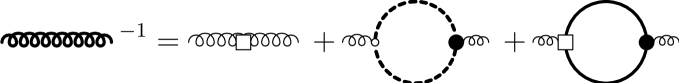
Figure 2: Diagrammatic representation of the CRDSE (60) for the gluon propagator. The small empty dot denotes the bare ghost-gluon vertex $\widetilde{\Gamma}_{0}$ [Eq. (40)], and the thick dashed line stands for the full (dressed) ghost propagator. The empty square box connected to two (amputated) wavy lines represents the variational kernel $2\omega$, which equals the inverse bare gluon propagator.

III.5 Quark-Gluon Vertex CRDSE

The CRDSEs for the quark and gluon propagator, see Figs. 1 and 2, contain the full quark-gluon vertex $\bar{\Gamma}$ defined by Eq. (50) and denoted diagrammatically by a full dot connecting a gluon and two quark lines. In the DSEs of the functional integral approach in Landau gauge a substantial dressing of the quark-gluon vertex is required in order to obtain a sufficient amount of spontaneous breaking of chiral symmetry. Although in the present Hamiltonian approach in Coulomb gauge spontaneous breaking of chiral symmetry is triggered already by the non-abelian Coulomb interaction Adler:1984ri ; Watson:2011kv ; Pak:2011wu ; *Pak:2013uba [see Eq. (73) below] the obtained quark condensate, the corresponding order parameter, is far too small Adler:1984ri . It increases substantially when the quark-gluon coupling is included Pak:2011wu ; Pak:2013uba . However, the quark condensate obtained in Refs. Pak:2011wu ; Pak:2013uba using a bare quark-gluon vertex is still somewhat too small. At the moment it is unclear whether the missing strength of chiral symmetry breaking is due to the use of a bare quark-gluon vertex or due to the approximation for the propagators. In any case it seems worthwhile to investigate the dressing of the quark-gluon vertex; this is given by a CRDSE, which we will derive below.

Putting $f=\xi^{\dagger}A$ in Eq. (47a) and using $\langle A\rangle=0$ we have

$$\bigl{[}Q_{0}^{-1}(1,4)+\bar{\gamma}(1,4)\bigr{]}\mathopen{}\mathclose{{}\left\langle\xi(4)\,\xi^{\dagger}(2)\,A(3)}\right\rangle+\bar{\Gamma}_{0}(1,4;5)\mathopen{}\mathclose{{}\left\langle\xi(4)\,A(5)\,\xi^{\dagger}(2)\,A(3)}\right\rangle=0.$$ (61)

The four-point function can be expressed in terms of propagators and vertex functions in the standard fashion by Legendre transforming the generating functional of connected Green’s functions to the effective action Campagnari:2010wc

$$\langle\mathop{}\!\mathrm{e}^{jA+\eta^{\dagger}\xi+\xi^{\dagger}\eta}\rangle\equiv\mathop{}\!\mathrm{e}^{W[j,\eta^{\dagger},\eta]},\qquad\Gamma[A,\xi,\xi^{\dagger}]+W[j,\eta^{\dagger},\eta]=jA+\eta^{\dagger}\xi+\xi^{\dagger}\eta.$$

Taking appropriate derivatives of the effective action one finds for the two-quark-two-gluon expectation value

$$\langle A(1)\,A(2)\,\xi(3)\,\xi^{\dagger}(4)\rangle={} D(1,2)\,Q(3,4)$$

$$+D(1^{\prime},1)\,D(2^{\prime},2)\,Q(3,3^{\prime})\,Q(4^{\prime},4)\biggl{\{}-\bar{\Gamma}_{\bar{q}qAA}(3^{\prime},4^{\prime};1^{\prime},2^{\prime})$$

$$+\Gamma(1^{\prime},2^{\prime},5)D(5,5^{\prime})\bar{\Gamma}(3^{\prime},4^{\prime};5^{\prime})$$

$$+\bar{\Gamma}(3^{\prime},5;1^{\prime})Q(5,5^{\prime})\bar{\Gamma}(5^{\prime},4^{\prime};2^{\prime})+\bar{\Gamma}(3^{\prime},5;2^{\prime})Q(5,5^{\prime})\bar{\Gamma}(5^{\prime},4^{\prime};1^{\prime})\Bigr{]}\biggr{\}},$$

where the two-quark-two-gluon proper vertex is defined by

$$\bar{\Gamma}_{\bar{q}qAA}(3,4;1,2)=\frac{\delta^{4}\Gamma[A,\xi^{\dagger},\xi]}{\delta\xi(4)\,\delta\xi^{\dagger}(3)\,\delta A(2)\,\delta A(1)}\biggr{|}_{A=\xi^{\dagger}=\xi=0}.$$

This equation is diagrammatically represented in Fig. 3.

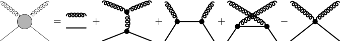
Figure 3: Vacuum expectation value of two gauge and two Grassmann fields.

Inserting this into Eq. (61) the CRDSE for the quark-gluon vertex becomes

$$\bar{\Gamma}(1,2;3)={} \bar{\Gamma}_{0}(1,2;3)$$

$$+\bar{\Gamma}_{0}(1,4;6^{\prime})Q(4,4^{\prime})\bar{\Gamma}(4^{\prime},5;3)Q(5,5^{\prime})\bar{\Gamma}(5^{\prime},2;6)D(6,6^{\prime})$$

$$+\bar{\Gamma}_{0}(1,4;6^{\prime})D(4,4^{\prime})\Gamma(4^{\prime},5,3)D(5,5^{\prime})\bar{\Gamma}(6,2;5^{\prime})Q(6^{\prime},6)$$

$$-\bar{\Gamma}_{0}(1,5;4)D(4,4^{\prime})Q(5,5^{\prime})\bar{\Gamma}_{\bar{q}qAA}(5^{\prime},2;4^{\prime},3).$$ (62)

Equation (III.5) is diagrammatically represented in Fig. 4.

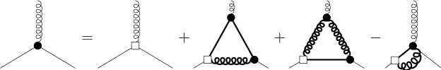
Figure 4: Diagrammatic representation of the DSE (III.5) for the quark-gluon vertex.

Let us also mention that another CRDSE for the quark-gluon vertex can be obtained by putting $f=AA$ in the gluonic CRDSE (47c). This results in

$$\bar{\Gamma}(1,2;3)={} \bar{\Gamma}_{0}(1,2;3)$$

$$+\bar{\Gamma}(1,4;6^{\prime})Q(4,4^{\prime})\bar{\Gamma}_{0}(4^{\prime},5;3)Q(5,5^{\prime})\bar{\Gamma}(5^{\prime},2;6)D(6,6^{\prime})$$

$$+\bar{\Gamma}_{\bar{q}\bar{q}qq}(1,4;2,5)Q(5,5^{\prime})Q(4^{\prime},4)\bar{\Gamma}_{0}(5^{\prime},4^{\prime};3)$$

$$-\Gamma_{\bar{q}q\bar{c}c}(1,2;4,5)G(5,5^{\prime})G(4^{\prime},4)\widetilde{\Gamma}_{0}(5^{\prime},4^{\prime};3),$$ (63)

which is diagrammatically shown in Fig. 5. Its new elements are a two-ghost-two-fermion vertex $\Gamma_{\bar{q}q\bar{c}c}$ and a four-fermion vertex $\bar{\Gamma}_{\bar{q}\bar{q}qq}$.

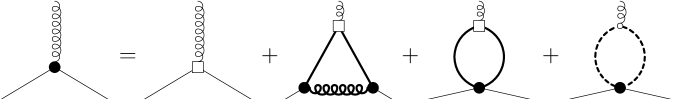
Figure 5: Alternative CRDSE (III.5) for the quark-gluon vertex resulting from the gluonic CRDSE (47c).

Both equations are equivalent as long as no approximations are introduced.

III.6 Ghost CRDSE

For the sake of completeness we quote here also the CRDSE for the ghost propagator, which was already derived in Refs. Feuchter:2004mk ; Campagnari:2010wc . To obtain this equation we do not need to explicitly introduce ghost fields. Rather, this equation can be obtained already from the operator identity

$$G_{A}(1,2)=G_{0}(1,2)-G_{0}(1,4)A(3)\,\widetilde{\Gamma}_{0}(4,5;3)\,G_{A}(4,2),$$

which follows from the definition of the Faddeev–Popov operator $G^{-1}_{A}$ [Eq. (31)] when this operator is inverted. Taking the VEV of this identity and using the definition Eq. (56) of the full ghost-gluon vertex we obtain the ghost CRDSE

$$G^{-1}(1,2)=G_{0}^{-1}(1,2)-\widetilde{\Gamma}_{0}(1,4;3)D(3,3^{\prime})G(4,4^{\prime})\widetilde{\Gamma}(4^{\prime},2;3^{\prime}),$$ (64)

which is diagrammatically represented in Fig. 6.

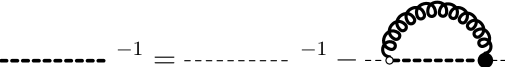
Figure 6: CRDSE (64) for the ghost propagator.

The CRDSEs for the higher $n$-point functions of the ghost field can be derived by representing the Faddeev-Popov determinant as a functional integral over the ghost fields and employing the standard DSE techniques, which we are using in the present paper for the quarks and the gluon fields.

The CRDSEs for the gluon and ghost propagators contain also the full ghost-gluon vertex, see Figs. 2 and 6. The CRDSE for this vertex was derived in Ref. Campagnari:2010wc and studied in Ref. Campagnari:2011bk . It was shown there that its dressing is negligible.

A final comment is in order concerning the CRDSEs derived in this section: For purely Gaussian wave functionals describing independent quasi-particles these CRDSEs become trivial and are not really necessary, since the higher-order correlation functions can be entirely expressed in terms of the two-point functions (propagators) by means of Wick’s theorem. However, for interacting theories treated beyond the mean-field approximation non-Gaussian wave functionals like our vacuum state [Eqs. (27) and (42)] necessarily emerge. Then the CRDSEs derived above allow us to express the various propagators of QCD in terms of the (so far unknown) variational kernels entering our ansatz for the vacuum wave functional. In Sect. IV we will use these equations to express the vacuum expectation value of the QCD Hamiltonian in terms of the variational kernels. In this way these CRDSEs enable us to carry out the variational principle for non-Gaussian wave functionals, which are required for interacting fields.

IV The QCD Vacuum Energy Density

With the CRDSEs at hand we are now in a position to express the vacuum expectation value of the QCD Hamiltonian in terms of the variational kernels. For this purpose we will first separate the various powers of the fields in the QCD Hamiltonian, so that their vacuum expectation value results in the various $n$-point functions.

The QCD Hamiltonian in Coulomb gauge is given by Christ:1980ku

$$H_{\mathrm{QCD}}=-\frac{1}{2}\int\mathop{}\!{\mathrm{d}^{3}}x\>\mathcal{J}_{A}^{-1}\frac{\delta}{\delta A_{i}^{a}(\vx)}\mathcal{J}_{A}\frac{\delta}{\delta A_{i}^{a}(\vx)}+\frac{1}{2}\int\mathop{}\!{\mathrm{d}^{3}}x\>\vB^{a}(\vx)\,\vB^{a}(\vx)\\ +\int\mathop{}\!{\mathrm{d}^{3}}x\>\psi^{n{\dagger}}(\vx)\bigl{[}-\mathrm{i}\mkern 1.0mu\alpha_{i}\partial_{i}+\beta m\bigr{]}\psi^{n}(\vx)-g\int\mathop{}\!{\mathrm{d}^{3}}x\>\psi^{m{\dagger}}(\vx)\alpha_{i}A_{i}^{a}(\vx)\,t^{a}_{mn}\psi^{n}(\vx)\\ +\frac{g^{2}}{2}\int\mathop{}\!{\mathrm{d}^{3}}x\mathop{}\!{\mathrm{d}^{3}}y\>\mathcal{J}_{A}^{-1}\rho^{a}(\vx)\mathcal{J}_{A}\,F_{A}^{ab}(\vx,\vy)\,\rho^{b}(\vy),$$ (65)

where $t^{a}$ are the generators of $\mathfrak{su}(N)$ in the fundamental representation, $\mathcal{J}_{A}$ is the Faddeev–Popov determinant [Eq. (30)], and

$$B_{k}^{a}(\vx)=\varepsilon_{kij}\mathopen{}\mathclose{{}\left(\partial_{i}A_{j}^{a}(\vx)+\frac{g}{2}f^{abc}A_{i}^{b}(\vx)\,A_{j}^{c}(\vx)}\right)$$

is the chromomagnetic field. Furthermore

$$F_{A}^{ab}(\vx,\vy)=\int\mathop{}\!{\mathrm{d}^{3}}z\>G_{A}^{ac}(\vx,\vz)\,(-\partial^{2}_{\vz})\,G_{A}^{cb}(\vz,\vy)$$ (66)

is the so-called Coulomb kernel, which arises from the resolution of Gauss’s law in Coulomb gauge, and

$$\rho^{a}(\vx)=f^{abc}A_{i}^{b}(\vx)\frac{\delta}{\mathrm{i}\,\delta A_{i}^{c}(\vx)}+\psi^{m{\dagger}}(\vx)t^{a}_{mn}\psi^{n}(\vx)$$

is the colour charge density, which we express as

$$\rho(1)=\rho_{A}(1)+\rho_{q}(1)\eqcolon R(2,3;1)\,A(2)\>\frac{\delta}{\mathrm{i}\,\delta A(3)}+\bar{R}(2,3;1)\,\psi^{\dagger}(2)\,\psi(3).$$

Here we have introduced the kernels

$$R(2,3;1) =f^{a_{1}a_{2}a_{3}}\,\delta_{i_{2}i_{3}}\,\delta(\vx_{1}-\vx_{2})\,\delta(\vx_{1}-\vx_{3}),$$ (67a)

$$\bar{R}(2,3;1) =t^{a_{1}}_{m_{2}m_{3}}\,\delta_{s_{2}s_{3}}\,\delta(\vx_{1}-\vx_{2})\,\delta(\vx_{1}-\vx_{3}).$$ (67b)

For later convenience we rewrite the total QCD Hamilton operator as

$$H_{\mathrm{QCD}}=H_{\mathrm{YM}}+H_{\mathrm{C}}^{qA}+H_{\mathrm{C}}^{qq}+H_{\mathrm{D}},\qquad H_{\mathrm{YM}}=H_{E}+H_{B}+H_{\mathrm{C}}^{AA}$$ (68)

and express the various terms in our compact notation. The kinetic (chromoelectric) part of the gauge field then reads

$$H_{E}=-\frac{1}{2}\mathcal{J}_{A}^{-1}\frac{\delta}{\delta A(1)}\mathcal{J}_{A}\frac{\delta}{\delta A(1)},$$

while the chromomagnetic part can be expressed as

$$H_{B}=\frac{1}{2}\int\mathop{}\!{\mathrm{d}^{3}}x\bigl{(}B^{a}_{i}(\vx)\bigr{)}^{2}=-\frac{1}{2}A(1)\Delta(1,2)A(2)+\frac{1}{3!}T(1,2,3)A(1)A(2)A(3)+\frac{1}{4!}T(1,2,3,4)A(1)A(2)A(3)A(4).$$ (69)

Here we have defined

$$\Delta(1,2)=\delta^{a_{1}a_{2}}\delta_{i_{1}i_{2}}\partial^{2}_{x_{1}}\delta(\vx_{1}-\vx_{2}).$$ (70)

Furthermore, the tensor structures $T(1,2,3)$ and $T(1,2,3,4)$ are irrelevant for the present work and can be found in Ref. Campagnari:2010wc . The non-abelian Coulomb interaction contains a pure Yang–Mills part

$$H_{\mathrm{C}}^{AA}=\frac{g^{2}}{2}\mathcal{J}_{A}^{-1}\rho_{A}(1)\mathcal{J}_{A}F_{A}(1,2)\,\rho_{A}(2),$$ (71)

a fermion-gluon interaction

$$H_{\mathrm{C}}^{qA}=\frac{g^{2}}{2}\mathopen{}\mathclose{{}\left[\mathcal{J}_{A}^{-1}\rho_{A}(1)\mathcal{J}_{A}F_{A}(1,2)\,\rho_{q}(2)+\rho_{q}(1)F_{A}(1,2)\,\rho_{A}(2)}\right],$$ (72)

and a fermionic Coulomb interaction

$$H_{\mathrm{C}}^{qq}=\frac{g^{2}}{2}\>\rho_{q}(1)\,F_{A}(1,2)\,\rho_{q}(2).$$ (73)

Finally, the one-particle quark Hamiltonian can be written as

$$H_{\mathrm{D}}=\psi^{\dagger}(1)\bigl{[}h_{0}(1,2)-J(1,2;3)\,A(3)\bigr{]}\psi(2)\equiv H^{(0)}_{\mathrm{D}}+H^{(1)}_{\mathrm{D}}$$ (74)

where $h_{0}$ is defined by Eq. (11) and we have introduced the bare quark-gluon vertex of the QCD Hamiltonian

$$J(1,2;3)=g\,t^{a_{3}}_{m_{1}m_{2}}\,(\alpha_{i_{3}})_{s_{1}s_{2}}\,\delta(\vx_{1}-\vx_{2})\,\delta(\vx_{1}-\vx_{3}).$$ (75)

To carry out the non-perturbative variational approach we now evaluate the expectation value of the QCD Hamiltonian Eq. (68) in the state defined by Eqs. (27), (41), and (42). We carry out this evaluation up to two-loop level, so that the corresponding equations of motion following from the variation of the energy will contain at most one loop. Let us emphasize, however, that loops are here defined in terms of the non-perturbative propagators and vertices.

The magnetic term $H_{B}$ [Eq. (69)] is insensitive to the quark part of the vacuum wave functional and hence yields the same contribution as in the pure Yang–Mills theory. Furthermore, the quark contribution to $\langle H_{\mathrm{C}}^{AA}\rangle$ [Eq. (71)] contains more than two loops, which we do not include here. Also the fermion-gluon Coulomb interaction $H^{qA}_{\mathrm{C}}$ [Eq. (72)] yields contributions only beyond two loops and is hence discarded.

When a Gaussian functional is used for the Yang–Mills sector [see Eqs. (27) and (28)] the cubic term of the magnetic energy Eq. (69) does not contribute. Furthermore, the quartic term gives rise to a tadpole in the gluonic gap equation Feuchter:2004mk , which can be absorbed into a renormalization constant. Note also that the contribution of the quartic term to the energy vanishes in dimensional regularization. Therefore in the following we will omit the cubic and quartic term of the magnetic energy Eq. (69), which then reduces to

$$\langle H_{B}\rangle=-\frac{1}{2}\Delta(1,2)D(2,1)$$ (76)

where $D(2,1)$ is the gluon propagator Eq. (51).

Due to overall translational invariance, the vacuum expectation value of the various terms of the Hamiltonian Eq. (65) always contains a diverging factor $(2\pi)^{3}\delta(\vp=0)$, which is nothing but the spatial volume $V$. This factor disappears when the energy density

$$e=\mathopen{}\mathclose{{}\left\langle H}\right\rangle/V$$

is considered.

IV.1 Single-Particle Hamiltonian

The vacuum expectation value of the single-particle quark Hamiltonian Eq. (74) is easily evaluated by means of Eq. (35)

$$\begin{split}\langle H_{\mathrm{D}}\rangle&=h_{0}(1,2)\mathopen{}\mathclose{{}\left\langle\psi^{\dagger}(1)\psi(2)}\right\rangle-J(1,2;3)\mathopen{}\mathclose{{}\left\langle\psi^{\dagger}(1)\psi(2)\,A(3)}\right\rangle\\ &=h_{0}(1,2)\bigl{[}\mathopen{}\mathclose{{}\left\langle\xi^{\dagger}(1)\xi(2)}\right\rangle+\Lambda_{+}(2,1)\bigr{]}-J(1,2;3)\bigl{[}\mathopen{}\mathclose{{}\left\langle\xi^{\dagger}(1)\xi(2)\,A(3)}\right\rangle+\Lambda_{+}(2,1)\langle A(3)\rangle\bigr{]}.\end{split}$$

Using $\langle A\rangle=0$ and the definition Eq. (50) of the full quark-gluon vertex $\bar{\Gamma}$ the above expression can be cast into the form

$$\langle H_{\mathrm{D}}\rangle=-h_{0}(1,2)[Q(2,1)-\Lambda_{+}(2,1)]-J(1,2;3)D(3,3^{\prime})Q(2,2^{\prime})\bar{\Gamma}(2^{\prime},1^{\prime};3^{\prime})Q(1^{\prime},1).$$ (77)

Here the last term arises from the direct coupling of the quarks to the gluons through the bare vertex $J(1,2;3)$ [Eq. (75)] in the QCD Hamiltonian. This term is diagrammatically represented in Fig. 7.

Figure 7: Diagrammatic representation of the last term in the r.h.s. of Eq. (77).

Besides the bare vertex $J$ it contains also the full quark-gluon vertex $\bar{\Gamma}$, whose CRDSEs have been derived in Sect. III.5 [Eqs. (III.5) and (III.5)]. These relate the full quark-gluon vertex via Eq. (46) to the fermionic variational kernels.

IV.2 Fermion-Fermion Coulomb Interaction

For the spontaneous breaking of chiral symmetry (SB$\chi$S) the quark part of the Coulomb interaction $H^{qq}_{\mathrm{C}}$ [Eq. (73)] seems to be crucial. This term alone triggers already SB$\chi$S Adler:1984ri , albeit not of sufficient strength. On the other hand it was shown in Refs. Pak:2011wu ; Pak:2013uba that the quark-gluon coupling (in $H_{\mathrm{D}}$) alone does not provide SB$\chi$S, at least within the approximation used in Refs. Pak:2011wu ; Pak:2013uba . However, the quark-gluon coupling in $H_{\mathrm{D}}$ substantially increases the amount of chiral symmetry breaking once $H_{\mathrm{C}}^{qq}$ is included Pak:2011wu ; Pak:2013uba .

The expectation value of the quark Coulomb interaction Eq. (73)

$$E_{\mathrm{C}}^{qq}\equiv\langle H_{\mathrm{C}}^{qq}\rangle =\frac{g^{2}}{2}\bar{R}(3,4;1)\bar{R}(5,6;2)\langle\psi^{\dagger}(3)\,\psi(4)\,F_{A}(1,2)\,\psi^{\dagger}(5)\,\psi(6)\rangle$$

is taken by means of Eq. (36), which yields

$$E_{\mathrm{C}}^{qq} =\frac{g^{2}}{2}\bar{R}(3,4;1)\bar{R}(5,6;2)\Bigl{\{}\begin{aligned} &\langle\xi^{\dagger}(3)\,\xi(4)\,F_{A}(1,2)\,\xi^{\dagger}(5)\,\xi(6)\rangle\\ &+\langle\xi^{\dagger}(3)\xi(4)F_{A}(1,2)\rangle\Lambda_{+}(6,5)+\langle\xi(4)\xi^{\dagger}(5)F_{A}(1,2)\rangle\Lambda_{+}(6,3)\\ &+\langle\xi^{\dagger}(5)\xi(6)F_{A}(1,2)\rangle\Lambda_{+}(4,3)+\langle\xi^{\dagger}(3)\xi(6)F_{A}(1,2)\rangle\Lambda_{-}(4,5)\\ &+\bigl{[}\Lambda_{+}(4,3)\Lambda_{+}(6,5)+\Lambda_{+}(6,3)\Lambda_{-}(4,5)\bigr{]}\langle F_{A}(1,2)\rangle\Bigr{\}}.\end{aligned}$$ (78)

Up to two loops in the energy we can replace the Coulomb kernel $F_{A}$ [Eq. (66)] by its (gluonic) vacuum expectation value $F\equiv\mathopen{}\mathclose{{}\left\langle F_{A}}\right\rangle$. Furthermore, since the Dirac projectors $\Lambda_{\pm}$ are the unit matrix in colour space their contraction with the kernels $\bar{R}$ [Eq. (67b)] of the quark colour charge density results in the trace of the generators of the gauge group, which vanishes. For this reason the second, fourth, and sixth term in the brackets on the r.h.s. of Eq. (78) vanish and we are left with

$$E_{\mathrm{C}}^{qq}\simeq\frac{g^{2}}{2}\bar{R}(3,4;1)\bar{R}(5,6;2)F(1,2)\Bigl{[}\mathopen{}\mathclose{{}\left\langle\xi(4)\,\xi^{\dagger}(3)\,\xi(6)\,\xi^{\dagger}(5)}\right\rangle+Q(4,5)\,\Lambda_{+}(6,3)-Q(6,3)\,\Lambda_{-}(4,5)+\Lambda_{+}(6,3)\,\Lambda_{-}(4,5)\Bigr{]}.$$ (79)

Finally, up to two-loop order in the energy it is sufficient to take the lowest order contribution to the fermion four-point function

$$\mathopen{}\mathclose{{}\left\langle\xi(4)\,\xi^{\dagger}(3)\,\xi(6)\,\xi^{\dagger}(5)}\right\rangle=Q(4,3)\,Q(6,5)-Q(4,5)\,Q(6,3)+\text{connected terms.}$$ (80)

Since the quark propagator $Q(1,2)$ is colour diagonal, when Eq. (80) is inserted into Eq. (79) the first term on the right-hand side of Eq. (80) gives also rise to a trace over the colour generators and thus to a vanishing contribution to the quark Coulomb energy Eq. (79), which then becomes

$$E_{\mathrm{C}}^{qq}\simeq-\frac{g^{2}}{2}\bar{R}(3,4;1)\bar{R}(5,6;2)F(1,2)\,\bigl{[}Q(4,5)+\Lambda_{-}(4,5)\bigr{]}\bigl{[}Q(6,3)-\Lambda_{+}(6,3)\bigr{]}.$$ (81)

IV.3 The Chromoelectric Energy

Contrary to the magnetic energy $\mathopen{}\mathclose{{}\left\langle H_{B}}\right\rangle$ and the gluonic Coulomb energy $\mathopen{}\mathclose{{}\left\langle H_{\mathrm{C}}^{AA}}\right\rangle$, the chromoelectric energy $\mathopen{}\mathclose{{}\left\langle H_{E}}\right\rangle$ does receive additional contributions from the quark sector at the considered two-loop order due to the quark-gluon coupling Eq. (43) in the fermionic wave functional Eq. (42). With the explicit form of the vacuum wave functional we find from Eq. (29) after an integration by parts with respect to the gluon field

$$\mathopen{}\mathclose{{}\left\langle H_{E}}\right\rangle =\frac{1}{2}\int\mathcal{D}A\,\mathcal{D}\xi^{\dagger}\,\mathcal{D}\xi\>\mathop{}\!\mathrm{e}^{-\mu}\mathopen{}\mathclose{{}\left[\frac{\delta}{\delta A(1)}\>\mathop{}\!\mathrm{e}^{-S_{f}^{*}-\frac{1}{2}S_{A}}}\right]\mathcal{J}_{A}\frac{\delta}{\delta A(1)}\mathop{}\!\mathrm{e}^{-S_{f}-\frac{1}{2}S_{A}}$$

$$=\frac{1}{2}\mathopen{}\mathclose{{}\left\langle\mathopen{}\mathclose{{}\left[\frac{\delta S_{f}^{*}}{\delta A(1)}+\frac{1}{2}\frac{\delta S_{A}}{\delta A(1)}}\right]\mathopen{}\mathclose{{}\left[\frac{\delta S_{f}}{\delta A(1)}+\frac{1}{2}\frac{\delta S_{A}}{\delta A(1)}}\right]}\right\rangle$$

$$=\frac{1}{8}\mathopen{}\mathclose{{}\left\langle\frac{\delta S_{A}}{\delta A(1)}\frac{\delta S_{A}}{\delta A(1)}}\right\rangle+\frac{1}{4}\mathopen{}\mathclose{{}\left\langle\frac{\delta S_{A}}{\delta A(1)}\frac{\delta(S_{f}+S_{f}^{*})}{\delta A(1)}}\right\rangle+\frac{1}{2}\mathopen{}\mathclose{{}\left\langle\frac{\delta S_{f}^{*}}{\delta A(1)}\frac{\delta S_{f}}{\delta A(1)}}\right\rangle.$$ (82)

To work out the remaining vacuum expectation values we use here the CRDSEs derived in Sec. III.1. For this purpose, using $S=S_{A}+S_{f}+S_{f}^{*}+\mu$ [see Eq. (38)] and $\delta\mu/\delta A=0$, we rewrite the general CRDSE (39) as

$$\mathopen{}\mathclose{{}\left\langle\frac{\delta S_{A}}{\delta A(1)}\>f}\right\rangle=\mathopen{}\mathclose{{}\left\langle\frac{\delta f}{\delta A(1)}}\right\rangle-\mathopen{}\mathclose{{}\left\langle\frac{\delta(S_{f}+S_{f}^{*})}{\delta A(1)}\>f}\right\rangle+\widetilde{\Gamma}_{0}(3,2;1)\langle G_{A}(2,3)f\rangle.$$ (83)

For the first two terms in Eq. (82) we use this CRDSE with $f=\delta S_{A}/\delta A$ and obtain

$$\mathopen{}\mathclose{{}\left\langle\frac{\delta S_{A}}{\delta A(1)}\frac{\delta S_{A}}{\delta A(1)}}\right\rangle+2\mathopen{}\mathclose{{}\left\langle\frac{\delta S_{A}}{\delta A(1)}\frac{\delta(S_{f}+S_{f}^{*})}{\delta A(1)}}\right\rangle$$

$$=\mathopen{}\mathclose{{}\left\langle\frac{\delta^{2}S_{A}}{\delta A(1)\,\delta A(1)}}\right\rangle+\widetilde{\Gamma}_{0}(3,2;1)\mathopen{}\mathclose{{}\left\langle G_{A}(2,3)\frac{\delta S_{A}}{\delta A(1)}}\right\rangle+\mathopen{}\mathclose{{}\left\langle\frac{\delta(S_{f}+S_{f}^{*})}{\delta A(1)}\frac{\delta S_{A}}{\delta A(1)}}\right\rangle.$$ (84)

For the last term we can again use Eq. (83) putting $f=\delta(S_{f}+S_{f}^{*})/\delta A$, yielding

$$\mathopen{}\mathclose{{}\left\langle\frac{\delta(S_{f}+S_{f}^{*})}{\delta A(1)}\frac{\delta S_{A}}{\delta A(1)}}\right\rangle=\mathopen{}\mathclose{{}\left\langle\frac{\delta^{2}(S_{f}+S_{f}^{*})}{\delta A(1)\,\delta A(1)}}\right\rangle+\widetilde{\Gamma}_{0}(3,2;1)\mathopen{}\mathclose{{}\left\langle G_{A}(2,3)\frac{\delta(S_{f}+S_{f}^{*})}{\delta A(1)}}\right\rangle-\mathopen{}\mathclose{{}\left\langle\frac{\delta(S_{f}+S_{f}^{*})}{\delta A(1)}\frac{\delta(S_{f}+S_{f}^{*})}{\delta A(1)}}\right\rangle.$$

Inserting this expression into Eq. (84) we obtain

$$\mathopen{}\mathclose{{}\left\langle\frac{\delta S_{A}}{\delta A(1)}\frac{\delta S_{A}}{\delta A(1)}}\right\rangle+2\mathopen{}\mathclose{{}\left\langle\frac{\delta S_{A}}{\delta A(1)}\frac{\delta(S_{f}+S_{f}^{*})}{\delta A(1)}}\right\rangle\\ =\mathopen{}\mathclose{{}\left\langle\frac{\delta^{2}S}{\delta A(1)\,\delta A(1)}}\right\rangle+\widetilde{\Gamma}_{0}(3,2;1)\mathopen{}\mathclose{{}\left\langle G_{A}(2,3)\frac{\delta S}{\delta A(1)}}\right\rangle-\mathopen{}\mathclose{{}\left\langle\frac{\delta(S_{f}+S_{f}^{*})}{\delta A(1)}\frac{\delta(S_{f}+S_{f}^{*})}{\delta A(1)}}\right\rangle.$$

Using the above derived expressions we can finally write the Yang–Mills chromoelectric energy Eq. (82) as

$$\langle H_{E}\rangle=\frac{1}{8}\mathopen{}\mathclose{{}\left\langle\frac{\delta^{2}S}{\delta A(1)\,\delta A(1)}}\right\rangle-\frac{1}{8}\mathopen{}\mathclose{{}\left\langle\frac{\delta(S_{f}-S_{f}^{*})}{\delta A(1)}\frac{\delta(S_{f}-S_{f}^{*})}{\delta A(1)}}\right\rangle+\frac{1}{8}\widetilde{\Gamma}_{0}(3,2;1)\mathopen{}\mathclose{{}\left\langle G_{A}(2,3)\frac{\delta S}{\delta A(1)}}\right\rangle.$$ (85)

Equation (85) is, so far, exact. Restricting ourselves to the Gaussian ansatz for the gluonic part of vacuum wave functional [see Eq. (41)] the various terms can be explicitly calculated. In the last term the definition of the ghost-gluon vertex [Eq. (56)] has to be used. One finds then for the chromoelectric energy

$$\mathopen{}\mathclose{{}\left\langle H_{E}}\right\rangle=E_{E}^{\mathrm{YM}}+E_{E}^{\mathrm{Q}},$$ (86)

where

$$E_{E}^{\mathrm{YM}}=\frac{1}{4}\bigl{[}\Omega(1,2)-\chi(1,2)\bigr{]}\Omega^{-1}(2,3)\bigl{[}\Omega(3,1)-\chi(3,1)\bigr{]}$$ (87)

is the contribution arising from the pure Yang–Mills sector, and

$$E_{E}^{\mathrm{Q}}=-\frac{1}{4}\>\sigma(1,1)+\frac{1}{4}\>\sigma_{-}(1,1)$$ (88)

is the explicit contribution of the quarks to the kinetic energy of the gluons. In Eq. (88) $\sigma_{-}$ is defined analogously to $\sigma$ [Eq. (58)], however, with the bare and full quark gluon vertex, $\bar{\Gamma}_{0}$ and $\bar{\Gamma}$, both replaced by

$$\bar{\Gamma}_{-}(1,2;3)=\Lambda_{+}(1,1^{\prime})\,K(1^{\prime},2^{\prime};3)\,\Lambda_{-}(2^{\prime},2)-\Lambda_{-}(1,1^{\prime})\,K^{\dagger}(1^{\prime},2;3)\,\Lambda_{+}(2^{\prime},2).$$ (89)

[This follows from the terms $S_{f}-S_{f}^{*}$ in Eq. (85).] Using the properties Eq. (13) of the projectors $\Lambda_{\pm}$ and Eq. (24), the quantity $\bar{\Gamma}_{-}$ [Eq. (89)] can be written as

$$\bar{\Gamma}_{-}(1,2;3)=Q_{0}(1,1^{\prime})\,\bar{\Gamma}_{0}(1^{\prime},2;3)=-\bar{\Gamma}_{0}(1,2^{\prime};3)\,Q_{0}(2^{\prime},2).$$ (90)

IV.4 The Total Energy

For carrying out the variation of the energy let us summarize the various energy contributions. To the order of approximation considered in the present work (two loops in the energy) the total energy is given by [cf. Eq. (68)]

$$E_{\mathrm{QCD}}\equiv\langle H_{\mathrm{QCD}}\rangle\simeq\langle H_{\mathrm{YM}}\rangle+\langle H_{\mathrm{D}}\rangle+\langle H_{\mathrm{C}}^{qq}\rangle,$$ (91)

with

$$\langle H_{\mathrm{YM}}\rangle=\langle H_{E}\rangle+\langle H_{B}\rangle+\langle H_{\mathrm{C}}^{AA}\rangle.$$

Here $\langle H_{B}\rangle$, $\langle H_{\mathrm{D}}\rangle$, $\langle H_{\mathrm{C}}^{qq}\rangle$, and $\langle H_{E}\rangle$ are given by Eqs. (76), (77), (81), and (86), respectively. Furthermore, the expression for $\langle H_{\mathrm{C}}^{AA}\rangle$ was given in Ref. Feuchter:2004mk . As shown in Ref. Heffner:2012sx , on a quantitative level this quantity is completely irrelevant and will hence be ignored in the following. For subsequent considerations it will be convenient to rewrite the energy Eq. (91) in the form

$$E_{\mathrm{QCD}}=E_{\mathrm{YM}}+E_{\mathrm{Q}}\,,$$

where

$$E_{\mathrm{YM}}=E_{E}^{\mathrm{YM}}+\langle H_{B}\rangle$$

is the energy of the Yang–Mills sector, for which we get from Eqs. (76) and (87)

$$E_{\mathrm{YM}}=\frac{1}{2}\Bigl{[}\frac{1}{2}D^{-1}(1,2)-\chi(1,2)\Bigr{]}D(2,3)\Bigl{[}\frac{1}{2}D^{-1}(3,1)-\chi(3,1)\Bigr{]}-\frac{1}{2}\Delta(1,2)D(2,1).$$

The energy of the quarks is given by

$$E_{\mathrm{Q}}=\langle H_{\mathrm{D}}\rangle+E_{\mathrm{C}}^{qq}+E_{E}^{\mathrm{Q}}$$ (92)

where the Dirac energy $\langle H_{\mathrm{D}}\rangle=E_{\mathrm{D}}^{(0)}+E_{\mathrm{D}}^{(1)}$ was given in Eq. (77). Furthermore, the quark energy Eq. (92) includes the quark contribution to the chromoelectric energy $E_{E}^{\mathrm{Q}}$ [Eq. (88)] as well as the non-abelian Coulomb interaction of the quarks [Eq. (81)].

The expressions given above for the quark energy can be substantially simplified by noticing that they consist of linear chains of fermionic matrices which are connected by ordinary matrix multiplication. Therefore, without loss of information we can skip the fermionic indices (but keep the bosonic ones) and assume ordinary matrix multiplication for the fermionic objects. This we will do in the rest of this paper’s body. The quark energy Eq. (92) is then given by

$$E_{\mathrm{Q}}={} -\operatorname{Tr}\bigl{[}h_{0}\bigl{(}Q-\tfrac{1}{2}Q_{0}\bigr{)}\bigr{]}-D(1,2)\operatorname{Tr}\bigl{[}J(1)Q\bar{\Gamma}(2)Q\bigr{]}$$

$$-\frac{1}{8}\operatorname{Tr}\bigl{[}\bar{\Gamma}_{0}(1)Q\bar{\Gamma}(1)Q\bigr{]}-\frac{1}{8}\operatorname{Tr}\bigl{[}Q_{0}\bar{\Gamma}_{0}(1)Q\bar{\Gamma}_{0}(1)Q_{0}Q\bigr{]}$$

$$-\frac{g^{2}}{2}\,F(1,2)\operatorname{Tr}\bigl{[}\bar{R}(1)\bigl{(}Q-\tfrac{1}{2}Q_{0}\bigr{)}\bar{R}(2)\bigl{(}Q-\tfrac{1}{2}Q_{0}\bigr{)}-\tfrac{1}{4}\bar{R}(1)\bar{R}(2)\bigr{]},$$ (93)

the trace being over fermionic indices only.

Above we have succeeded to express the vacuum expectation value of the QCD Hamiltonian in terms of the variational kernels (denoted graphically by open square boxes) and the various $n$-point functions (denoted graphically by full dots), the latter being themselves functionals of the variational kernels through the CRDSEs. In addition, the energy contains the bare vertices of the QCD Hamiltonian, denoted graphically by open circles.

We are now in a position to carry out the variation of the energy. This will result in a set of gap equations, which have to be solved together with the CRDSEs.

V The Variational Principle

Our trial wave functional [see Eqs. (27), (41)–(43)] contains three variational kernels: $\omega$ of the Yang–Mills wave functional, and $K_{0}$ and $K$ of the quark wave functional. In carrying out the variations with respect to these kernels we will ignore implicit dependences which will give rise to higher-order loops in the resulting gap equations. This implies in particular that we will ignore the dependence of the ghost propagator (and hence of $\chi$) on the gluon kernel, as we did already previously in the treatment of the Yang–Mills sector Feuchter:2004mk . In the same spirit we will ignore the dependence of the gluon propagator on the fermionic kernels $K_{0}$ and $K$ as well as the implicit dependence of the quark propagator on $\omega$ with the exception of the free single-particle energy $E_{\mathrm{D}}^{(0)}$ [Eq. (77)], where we will include the dependence of $Q$ on the gluon propagator, since this contributes only a one-loop term to the gap equation. The explicit derivation of the gap equations is given in App. B.

The variational equation with respect to $\omega$ can be combined with the CRDSE (60) as explained in App. B, resulting in

$$\Omega^{2}(1,2)=-\Delta(1,2)+\chi^{2}(1,2)-2\operatorname{Tr}\bigl{[}\bar{\Gamma}(1)\,Q\,J(2)\,Q\bigr{]}-2\operatorname{Tr}\bigl{[}\bar{\Gamma}(1)\,Q\,h_{0}Q\bar{\Gamma}_{0}(2)Q\bigr{]}.$$ (94)

Here the trace is over the fermionic indices only, as it should be clear from the context. Furthermore, $\Delta(1,2)$ is the Laplacian Eq. (70), $\chi$ is the ghost loop [Eq. (57)], $Q$ is the full quark propagator [Eq. (48)], $J$ [Eq. (75)] is the quark-gluon coupling of the QCD Hamiltonian, and $\bar{\Gamma}_{0}$ [Eq. (46)] is the quark-gluon variational kernel of our trial wave functional Eq. (27). Finally, $\bar{\Gamma}$ is the corresponding dressed quark-gluon vertex Eq. (50), which is related to the bare one $\bar{\Gamma}_{0}$ by the CRDSE (III.5) [or Eq. (III.5)]. Equation (94) generalizes the gluonic gap equation obtained in Refs. Feuchter:2004mk ; Campagnari:2010wc to full QCD and is diagrammatically represented in Fig. 8.

Figure 8: Diagrammatic representation of Eq. (94). Small open circles represent the “vertices” occurring in the Hamiltonian.

Note that the quarks contribute threefold to this equation: i) through the last but one term, which is a quark loop arising from the quark-gluon coupling in the QCD Hamiltonian, ii) through the last term, which is a quark loop arising from the free quark energy due to the dependence of the quark propagator on the gluon propagator [see Eq. (98) below], and iii) through the quark loop $\sigma$ [Eq. (58)] entering the gluon CRDSE (60) for $\Omega$. The latter arises entirely from the quark-gluon coupling $\bar{\Gamma}_{0}$ in the QCD wave functional. In App. C the gluon gap equation (94) is used to simplify the expression for the stationary energy of the QCD vacuum, which will be needed in future investigations.

The variation with respect to the biquark kernel $K_{0}$ leads to the conditions

$$\Lambda_{-}QhQ\Lambda_{+}=0,\qquad\Lambda_{+}QhQ\Lambda_{-}=0,$$ (95)

where $h=-\delta E_{\mathrm{QCD}}/\delta Q$ is an effective single-quark Hamiltonian

$$h=h_{0} +D(1,2)\bigl{[}J(1)Q\bar{\Gamma}(2)+\bar{\Gamma}(1)QJ(2)\bigr{]}$$

$$+\frac{1}{8}\Bigl{\{}\bar{\Gamma}_{0}(1)Q\bar{\Gamma}(1)+\bar{\Gamma}(1)Q\bar{\Gamma}_{0}(1)\Bigr{\}}+\frac{1}{4}\,Q_{0}\bar{\Gamma}_{0}(1)Q\bar{\Gamma}_{0}(1)Q_{0}$$

$$+g^{2}F(1,2)\bar{R}(1)\bigl{[}Q-\tfrac{1}{2}Q_{0}\bigr{]}\bar{R}(2).$$ (96)

The quark gap equations are shown diagrammatically in Fig. 9.

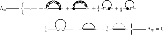
Figure 9: Diagrammatic representation of the quark equation resulting from Eqs. (95) and (V). The double line represents the Coulomb propagator $F\equiv\langle F_{A}\rangle$ [Eq. (66)].

In the effective single-particle Hamiltonian, $h_{0}$ is the Dirac Hamiltonian of free fermions while the remaining terms on the r.h.s. have all the same structure: the quark propagator $Q$ (or its free counterpart $Q_{0}$) is sandwiched by quark-gluon couplings: $J$ is the quark-gluon coupling in the QCD Dirac Hamiltonian, $\bar{\Gamma}_{0}$ and $\bar{\Gamma}$ are, respectively, bare and dressed quark-gluon kernels of our QCD wave functional, and $\bar{R}$ [Eq. (67b)] is the coupling vertex of the quarks to the Coulomb kernel.

The variation of the energy with respect to the vector kernel $K$ or $K^{\dagger}$ is carried out in App. B.3. Thereby the CRDSE (III.5) is used to find the variation of the full (dressed) quark-gluon vertex with respect to the kernels $K$, $K^{\dagger}$. For simplicity, we quote here the resulting variational equations for $K$, $K^{\dagger}$ only in the bare-vertex approximation [Eq. (B.3)]

$$\Lambda_{\pm}\,Q\bigl{\{}\Lambda_{\pm}\bar{\Gamma}_{0}(1)+2D(1,2)\bigl{[}J(2)+h_{0}Q\bar{\Gamma}_{0}(2)+\bar{\Gamma}_{0}(2)Qh_{0}\bigr{]}\bigr{\}}Q\Lambda_{\mp}=0,$$ (97)

which is represented diagrammatically in Fig. 10. The kernel $K$ enters here through the bare quark-gluon vertex $\bar{\Gamma}_{0}$ [Eq. (46)].

Figure 10: Diagrammatic representation of the gap equation (97) for the vector kernel.

In fact, Eq. (97) can be explicitly solved for $K$ Campagnari:tbp .

Equations (94), (V), and (97) provide the gap equations for the variational kernels of our trial ansatz given by Eqs. (27), (41) and (42) for the QCD vacuum wave functional. These equations have to be solved together with the CRDSEs for the various propagators and vertices occurring in the variational equations. In a first step one will use the bare vertex approximation, which results in an explicit expression for the vector kernel $K(1,2;3)$ in terms of the quark and gluon propagators. Furthermore, one will do a quenched calculation using the gluon propagator (known from the present approach to the Yang–Mills sector and also from the lattice calculation) as input for the quark sector. Such calculations are presently carried out.

VI Conclusions

The variational approach to the Hamiltonian formulation of interacting quantum field theories proposed in Ref. Campagnari:2010wc and developed there for Yang–Mills theory was extended to full QCD. The main feature of this approach is the use of CRDSEs to express the vacuum expectation values of powers of field operators (i.e., $n$-point functions) in terms of the variational kernels occurring in the exponent of the vacuum wave functional. In this way the variational approach can be carried out for non-Gaussian wave functionals, i.e., for interacting quantum field theories. To make use of the standard DSE techniques this approach requires the use of the coherent fermion state basis of Fock space, which is expressed in terms of Grassmann variables.

Assuming a vacuum wave functional which contains the coupling of the quarks to the gluons we have derived the necessary CRDSEs. By means of these CRDSEs we have expressed the vacuum expectation value of the QCD-Hamiltonian in Coulomb gauge in terms of the variational kernels of the wave functionals and carried out the variation of the energy, resulting in a set of so-called gap equations. These gap equations have to be solved together with the pertinent CRDSEs.

At first sight it seems that the present variational approach is quite cumbersome and less economic than the conventional DSE approach in the functional integral formulation of QCD in Landau gauge Alkofer:2000wg ; Fischer:2008uz ; Binosi:2009qm . There one has to solve the standard DSEs where the bare vertices are defined by the classical action of QCD. In the present approach we have to solve the CRDSEs, which are structurally similar to (and at least as complicated as) the usual DSEs. Moreover, contrary to the usual DSEs the bare vertices in the CRDSEs are not known a priori but are variational kernels, which have to be found by solving the gap equations. So it seems that our variational approach is much more expensive than the conventional DSE approach to QCD in Landau gauge. However, the infinite tower of DSEs has to be truncated for practical reasons and there is usually little control over the quality of the approximation achieved. Also in our approach we have to truncate the tower of CRDSEs. However, whatever truncation we use, the variational principle (i.e., the gap equations) will provide us with the optimal choice of bare vertices for that truncation. We can therefore expect that the “bare” vertices of the CRDSEs, i.e., the variational kernels, capture some of the physics lost by the corresponding truncation of the usual DSEs. In fact our “bare” vertices obtained by solving the gap equations are not at all “bare” but resemble more dressed vertices of the usual DSE approach Campagnari:tbp . As an illustrative example consider the quark-gluon vertex. In the conventional DSE approach in Landau gauge no chiral symmetry breaking is obtained when a bare quark-gluon vertex is used in the quark DSE. In our approach we do get chiral symmetry breaking even in the bare-vertex approximation.

In the future we plan to use the approach developed in this paper for a realistic description of the spontaneous breaking of chiral symmetry in the QCD vacuum. Furthermore, we intend to extend this approach to QCD at finite temperature and finite baryon density.

The present approach is quite general and in principle can be applied to any interacting quantum field theory as well as to interacting many-body systems.

Appendix A Diagrammatics

Propagators:

$$\equiv\;Q(1,2)\qquad$$  [Eq. (48)]

$$\equiv\;\bar{\gamma}(1,2)$$  [Eq. (44)]

$$\equiv\;D(1,2)$$  [Eq. (51)]

$$\equiv\;2\omega(1,2)$$  [Eq. (41)]

$$\equiv\;h_{0}(1,2)$$  [Eq. (11)]

$$\equiv\;\langle F_{A}(1,2)\rangle$$  [Eq. (66)]

Vertices:

$$\equiv\;J(1,2;3)\quad \equiv\;\bar{R}(1,2;3)\quad$$  [Eq. (75)]  [Eq. (67b)]

$$\equiv\;\bar{\Gamma}_{0}(1,2;3) \equiv\;\bar{\Gamma}(1,2;3)$$  [Eq. (46)]  [Eq. (50)]

$$\equiv\;\widetilde{\Gamma}_{0}(1,2;3) \equiv\;\widetilde{\Gamma}(1,2;3)$$  [Eq. (40)]  [Eq. (56)]

Appendix B Derivation of the Variational Equations

Below we explicitly carry out the variation of the QCD vacuum energy density with respect to the variational kernels $\omega$, $K_{0}$, $K$ of our trial ansatz [see Eqs. (41)–(43)] for the QCD vacuum wave functional.

B.1 The Gluon Gap Equation

If the implicit dependence of the ghost and quark loop, $\chi$ and $\sigma$, on the gluon propagator is ignored, from the gluon CRDSE (60) it is seen that the variation with respect to $\omega$ can be traded for the variation with respect to $\Omega$ or, more conveniently, with respect to the gluon propagator $D$ [Eq. (59)].

From the quark CRDSE (52) we have

$$\frac{\delta Q^{-1}(1,2)}{\delta D(3,4)}=-\bar{\Gamma}_{0}(1,5;3)Q(5,6)\bar{\Gamma}(6,2;4)$$ (98)

resulting in

$$\frac{\delta E_{\mathrm{D}}^{(0)}}{\delta D(3,4)}=h_{0}(2,1)Q(1,1^{\prime})\frac{\delta Q^{-1}(1^{\prime},2^{\prime})}{\delta D(3,4)}Q(2^{\prime},2)=-h_{0}(2,1)Q(1,1^{\prime})\bar{\Gamma}_{0}(1^{\prime},5;3)Q(5,6)\bar{\Gamma}(6,2^{\prime};4)Q(2^{\prime},2).$$ (99)

Minimization of $E_{\mathrm{QCD}}$ with respect to $D(1,2)$ then yields the condition

$$\Bigl{[}-\frac{1}{2}D^{-1}(3,1)D^{-1}(2,4)\Bigr{]}D(4,5)\Bigl{[}\frac{1}{2}D^{-1}(5,3)-\chi(5,3)\Bigr{]}\\ +\frac{1}{2}\Bigl{[}\frac{1}{2}D^{-1}(3,1)-\chi(3,1)\Bigr{]}\Bigl{[}\frac{1}{2}D^{-1}(2,3)-\chi(2,3)\Bigr{]}-\frac{1}{2}\Delta(2,1)\\ -h_{0}(3,4)Q(4,1^{\prime})\bar{\Gamma}_{0}(1^{\prime},5;1)Q(5,6)\bar{\Gamma}(6,3^{\prime};2)Q(3^{\prime},3)-J(3,4;1)Q(4,5)\bar{\Gamma}(5,6;2)Q(6,3)=0$$ (100)

Expressing the gluon propagator Eq. (59) by the gluon energy $\Omega$ this equation can be simplified to

$$\Omega^{2}(1,2)=-\Delta(1,2)+\chi^{2}(1,2)-2\bar{\Gamma}(5,6;1)Q(6,3)J(3,4;2)Q(4,5)-2\bar{\Gamma}(6,3^{\prime};1)Q(3^{\prime},3)h_{0}(3,4)Q(4,4^{\prime})\bar{\Gamma}_{0}(4^{\prime},5;2)Q(5,6).$$

If we suppress the fermionic indices we arrive at Eq. (94).

B.2 The Quark Gap Equation

The energy depends on the scalar kernel $K_{0}$ only through the quark propagator $Q$. Hence the variation with respect to $K_{0}$ and $K_{0}^{\dagger}$ can be carried out as

$$\frac{\delta E_{\mathrm{QCD}}}{\delta K_{0}(2,1)}=\frac{\delta E_{\mathrm{QCD}}}{\delta Q(4,3)}\frac{\delta Q(4,3)}{\delta K_{0}(2,1)}\overset{!}{=}0,\qquad\frac{\delta E_{\mathrm{QCD}}}{\delta K_{0}^{\dagger}(2,1)}=\frac{\delta E_{\mathrm{QCD}}}{\delta Q(4,3)}\frac{\delta Q(4,3)}{\delta K_{0}^{\dagger}(2,1)}\overset{!}{=}0.$$ (101)

From the quark CRDSE (52) and Eq. (45) we have

$$\frac{\delta Q(4,3)}{\delta K_{0}(2,1)}=-Q(4,4^{\prime})\Lambda_{+}(4^{\prime},2)\Lambda_{-}(1,3^{\prime})Q(3^{\prime},3),\qquad\frac{\delta Q(4,3)}{\delta K_{0}^{\dagger}(2,1)}=-Q(4,4^{\prime})\Lambda_{-}(4^{\prime},2)\Lambda_{+}(1,3^{\prime})Q(3^{\prime},3),$$

where we have included only the explicit $K_{0}$ dependence, since the implicit $K_{0}$ dependence of $Q$ in the last term of Eq. (52) would lead to two-loop terms in Eq. (101). Defining

$$\frac{\delta E_{\mathrm{QCD}}}{\delta Q(2,1)}=-h(1,2)$$ (102)

the stationary condition Eq. (101) becomes

$$\Lambda_{-}(1,3)Q(3,3^{\prime})h(3^{\prime},4^{\prime})Q(4^{\prime},4)\Lambda_{+}(4,2)=0,\qquad\Lambda_{+}(1,3)Q(3,3^{\prime})h(3^{\prime},4^{\prime})Q(4^{\prime},4)\Lambda_{-}(4,2)=0.$$ (103)

The quantity $h(1,2)$ [Eq. (102)] defines an effective quasi-particle Hamiltonian of the quarks. Restricting ourselves also up to including one-loop terms in the quark gap equation (103) only those terms contribute to $h(1,2)$ which explicitly depend on the quark propagator, i.e., the quark energy Eq. (92) of (IV.4). We find then

$$h(1,2)=h_{0}(1,2)+J(1,3;4)Q(3,3^{\prime})\bar{\Gamma}(3^{\prime},2;4^{\prime})D(4,4^{\prime})+\bar{\Gamma}(1,3;4)Q(3,3^{\prime})J(3^{\prime},2;4^{\prime})D(4,4^{\prime})\\ +\frac{1}{8}\Bigl{\{}\bar{\Gamma}_{0}(1,3;4)Q(3,3^{\prime})\bar{\Gamma}(3^{\prime},2;4)+\bar{\Gamma}(1,3;4)Q(3,3^{\prime})\bar{\Gamma}_{0}(3^{\prime},2;4)-\bigl{(}\bar{\Gamma}_{0}\to\bar{\Gamma}_{-},\bar{\Gamma}\to\bar{\Gamma}_{-}\bigr{)}\Bigr{\}}\\ +g^{2}F(4,4^{\prime})\bar{R}(1,3;4)\bigl{[}Q(3,3^{\prime})-\tfrac{1}{2}Q_{0}(3,3^{\prime})\bigr{]}\bar{R}(3^{\prime},2;4^{\prime}),$$

where $\bar{\Gamma}_{-}$ is defined by Eq. (89). Using Eq. (90) we recover Eq. (V).

Equations (103) are matrix-valued equations. Since $\Lambda_{+}\Lambda_{-}=0$, the expressions on the l.h.s. of these equations are manifestly traceless. The relevant information can be extracted by multiplying these equations with Dirac matrices and taking the trace. All considerations given above are valid for massive bare quarks. The quark gap equations (103) simplify for massless bare quarks. For instance, multiplying Eqs. (103) with $\beta$ and taking the trace, thereby using $\beta\Lambda_{+}=\Lambda_{-}\beta$, which is valid for massless bare quarks, we obtain the two conditions

$$\operatorname{Tr}(QhQ\Lambda_{\pm}\beta)=0$$

which can be collected in

$$\operatorname{Tr}(QhQ\beta)=0.$$

B.3 The Equation of Motion for the Vector Kernel

Finally we derive the equation of motion for the vector kernel $K(1,2;3)$ [Eq. (43)] of the quark wave functional [Eqs. (27), (42)]. The energy depends explicitly on the vector kernel $K$ through the bare and full quark-gluon vertex [$\bar{\Gamma}_{0}$ Eq. (46) and $\bar{\Gamma}$ Eq. (50) respectively], and implicitly through the quark propagator $Q$. Restricting ourselves to one-loop terms in the equation of motion we can neglect this implicit dependence in all energy terms except in the free single-particle energy [first term on the r.h.s of Eq. (77)]. From the quark CRDSE (52) we get

$$\frac{\delta Q^{-1}(6,7)}{\delta K(1,2;3)}=-\frac{\delta\bar{\Gamma}_{0}(6,6^{\prime};8)}{\delta K(1,2;3)}\,Q(6^{\prime},7^{\prime})\,D(8,8^{\prime})\,\bar{\Gamma}(7^{\prime},7;8^{\prime})-\bar{\Gamma}_{0}(6,6^{\prime};8)\,Q(6^{\prime},7^{\prime})\,D(8,8^{\prime})\,\frac{\delta\bar{\Gamma}(7^{\prime},7;8^{\prime})}{\delta K(1,2;3)}\,.$$

The variation of the energy with respect to $K(1,2;3)$ yields therefore the following equation of motion (for $K^{\dagger}$)

$$0={} h_{0}(4,5)Q(5,6)\mathopen{}\mathclose{{}\left[\frac{\delta\bar{\Gamma}_{0}(6,6^{\prime};8)}{\delta K(1,2;3)}\,Q(6^{\prime},7^{\prime})\,\bar{\Gamma}(7^{\prime},7;8^{\prime})+\bar{\Gamma}_{0}(6,6^{\prime};8)\,Q(6^{\prime},7^{\prime})\,\frac{\delta\bar{\Gamma}(7^{\prime},7;8^{\prime})}{\delta K(1,2;3)}}\right]Q(7,4)\,D(8,8^{\prime})$$

$$+J(4,5;6)Q(5,7)\frac{\delta\bar{\Gamma}(7,8;9)}{\delta K(1,2;3)}Q(8,4)D(6,9)$$

$$+\frac{1}{8}\mathopen{}\mathclose{{}\left[\frac{\delta\bar{\Gamma}_{0}(4,5;6)}{\delta K(1,2;3)}Q(5,7)\bar{\Gamma}(7,8;6)+\bar{\Gamma}_{0}(4,5;6)Q(5,7)\frac{\delta\bar{\Gamma}(7,8;6)}{\delta K(1,2;3)}}\right]Q(8,4)$$

$$+\frac{1}{4}Q_{0}(4,5)\frac{\delta\bar{\Gamma}_{0}(5,6;7)}{\delta K(1,2;3)}Q(6,8)\bar{\Gamma}_{0}(8,9;7)Q_{0}(9,10)Q(10,4)$$ (104)

For the bare quark-gluon vertex we find from its definition Eq. (46)

$$\frac{\delta\bar{\Gamma}_{0}(4,5;6)}{\delta K(1,2;3)}=\Lambda_{+}(4,1)\delta(6,3)\Lambda_{-}(2,5),\qquad\frac{\delta\bar{\Gamma}_{0}(4,5;6)}{\delta K^{\dagger}(1,2;3)}=\Lambda_{-}(4,1)\delta(6,3)\Lambda_{+}(2,5).$$ (105)

On the other hand, from the CRDSE (III.5) for the full quark-gluon vertex $\bar{\Gamma}$, which in the condensed notation of Sec. IV.4 reads

$$\bar{\Gamma}(1)=\bar{\Gamma}_{0}(1)+\bar{\Gamma}_{0}(2)Q\bar{\Gamma}(1)Q\bar{\Gamma}(3)D(2,3)+\bar{\Gamma}_{0}(2)Q\bar{\Gamma}(3)D(2,2^{\prime})D(3,3^{\prime})\Gamma(2^{\prime},3^{\prime},1)-\bar{\Gamma}_{0}(2)Q\bar{\Gamma}_{\bar{q}qAA}(1,3)D(2,3)$$ (106)

we find the variation of the full quark-gluon vertex $\bar{\Gamma}$ with respect to the vector kernels $K$ and $K^{\dagger}$. In taking the variation of this equation with respect to $K$, $K^{\dagger}$ on the right-hand side we can replace the variation of the full vertices by those of the bare ones ($\delta\bar{\Gamma}/\delta K\to\delta\bar{\Gamma}_{0}/\delta K$). This is because the full vertices occur on the right-hand side of Eq. (106) only inside loops and the variation of their dressings would result in more than one loop. Since the variation if the bare vertices are explicitly known [see Eq. (105)], Eq. (106) provides us with an explicit expression for the variation of the full quark-gluon vertex, which has then to be inserted into Eq. (B.3). This completes the derivation of the variational equations for $K$ and ^†. For illustrative purposes we present here these equations also in the bare-vertex approximation, replacing the full vertex $\bar{\Gamma}$ by the bare one $\bar{\Gamma}_{0}$. The equation of motion (B.3) reduces then to

$$0=\Lambda_{-}Q\bigl{\{}{} D(1,2)\bigr{[}\bar{\Gamma}_{0}(2)Qh_{0}+h_{0}Q\bar{\Gamma}_{0}(2)+J(2)\bigr{]}$$

$$+\frac{1}{8}\bigl{[}2\bar{\Gamma}_{0}(1)+\bar{\Gamma}_{0}(1)Q_{0}-Q_{0}\bar{\Gamma}_{0}(1)\bigr{]}\bigr{\}}Q\Lambda_{+}.$$ (107)

Using Eq. (90) we can rewrite the last term as

$$2\bar{\Gamma}_{0}(1)+\bar{\Gamma}_{0}(1)Q_{0}-Q_{0}\bar{\Gamma}_{0}(1)=2(1-Q_{0})\bar{\Gamma}_{0}(1)=4\Lambda_{-}\bar{\Gamma}_{0}(1)$$

where we have used the definition (24) of $Q_{0}$ in terms of the projectors $\Lambda_{\pm}$.

Appendix C The stationary energy

For later application we simplify the expression for the energy at the stationary point. For this purpose we multiply Eq. (98) with $D(3,4)$ and use the quark CRDSE (52) to find

$$\frac{\delta Q^{-1}(1,2)}{\delta D(3,4)}D(3,4)=-\bar{\Gamma}_{0}(1,5;3)Q(5,6)\bar{\Gamma}(6,2;4)D(3,4)=Q^{-1}(1,2)-Q_{0}^{-1}(1,2)-\bar{\gamma}(1,2).$$

With this relation we obtain from Eq. (99)

$$\frac{\delta E_{\mathrm{D}}^{(0)}}{\delta D(3,4)}D(3,4)=h_{0}(2,1)\bigl{\{}Q(1,2)-Q(1,1^{\prime})\bigl{[}Q_{0}^{-1}(1^{\prime},2^{\prime})+\bar{\gamma}(1^{\prime},2^{\prime})\bigr{]}Q(2^{\prime},2)\bigr{\}}.$$ (108)

Multiplying now the gap equation (100) with $D(1,2)$ and using Eq. (108) we can express the sum of the Yang–Mills energy $E_{\mathrm{YM}}$ and quark-gluon interaction energy $E_{\mathrm{D}}^{(1)}$ as

$$\begin{split}E_{\mathrm{YM}}+E_{\mathrm{D}}^{(1)}&\equiv E_{E}^{\mathrm{YM}}+E_{B}+E_{\mathrm{D}}^{(1)}\\ &=\frac{1}{2}\bigl{[}\Omega(1,1)-\chi(1,1)\bigr{]}-h_{0}(1,2)Q(2,1)+h_{0}(2,2^{\prime})Q(2^{\prime},1^{\prime})\bigl{[}Q_{0}^{-1}(1^{\prime},1)+\bar{\gamma}(1^{\prime},1)\bigr{]}Q(1,2),\end{split}$$

where we have used in the last expression the quark CRDSE (52). Adding here also the free Dirac energy $E_{\mathrm{D}}^{(0)}$ we obtain

$$E_{\mathrm{YM}}+E_{\mathrm{D}}=\frac{1}{2}\bigl{[}\Omega(1,1)-\chi(1,1)\bigr{]}-h_{0}(2,1)\bigl{[}2Q(1,2)-\Lambda_{+}(1,2)\bigr{]}+h_{0}(1,1^{\prime})Q(1^{\prime},2^{\prime})\bigl{[}Q_{0}^{-1}(2^{\prime},2)+\bar{\gamma}(2^{\prime},2)\bigr{]}Q(2^{\prime},2)\bigr{]}.$$ (109)

Note that this expression holds only at the stationary point [i.e., for gluon propagators satisfying the gap equation (94)]. Formally, the first term on the r.h.s. of Eq. (109) is the same as the one obtained in Ref. Heffner:2012sx for the pure Yang–Mills sector. However, in the present case $\Omega$ is the solution of the gap equation (94), which contains the quark loop. Also $\chi$ [Eq. (57)], being a functional of $\Omega$ through the ghost propagator, will, of course, be different.

References

- (1) R. Alkofer and L. von Smekal, Phys. Rept. 353, 281 (2001), arXiv:hep-ph/0007355.
- (2) C. S. Fischer, J. Phys. G32, R253 (2006), arXiv:hep-ph/0605173.
- (3) C. S. Fischer, A. Maas, and J. M. Pawlowski, Annals Phys. 324, 2408 (2009), arXiv:0810.1987.
- (4) D. Binosi and J. Papavassiliou, Phys. Rept. 479, 1 (2009), arXiv:0909.2536.
- (5) D. Zwanziger, Nucl. Phys. B518, 237 (1998).
- (6) P. Watson and H. Reinhardt, Phys. Rev. D75, 045021 (2007), arXiv:hep-th/0612114.
- (7) P. Watson and H. Reinhardt, Phys. Rev. D76, 125016 (2007), arXiv:0709.0140.
- (8) P. Watson and H. Reinhardt, Phys. Rev. D77, 025030 (2008), arXiv:0709.3963.
- (9) C. Popovici, P. Watson, and H. Reinhardt, Phys. Rev. D79, 045006 (2009), arXiv:0810.4887.
- (10) H. Reinhardt and P. Watson, Phys. Rev. D79, 045013 (2009), arXiv:0808.2436.
- (11) P. Watson and H. Reinhardt, Eur. Phys. J. C65, 567 (2010), arXiv:0812.1989.
- (12) P. Watson and H. Reinhardt, Phys. Rev. D82, 125010 (2010), arXiv:1007.2583.
- (13) P. Watson and H. Reinhardt, Phys. Rev. D85, 025014 (2012), arXiv:1111.6078, 27 pages, 11 figures.
- (14) P. Watson and H. Reinhardt, Phys.Rev. D86, 125030 (2012), arXiv:1211.4507.
- (15) C. Popovici, P. Watson, and H. Reinhardt, Phys. Rev. D81, 105011 (2010), arXiv:1003.3863.
- (16) C. Popovici, P. Watson, and H. Reinhardt, Phys. Rev. D83, 025013 (2011), arXiv:1010.4254.
- (17) C. Popovici, P. Watson, and H. Reinhardt, Phys. Rev. D83, 125018 (2011), arXiv:1103.4786.
- (18) J. M. Pawlowski, Annals Phys. 322, 2831 (2007), arXiv:hep-th/0512261.
- (19) H. Gies, Lect. Notes Phys. 852, 287 (2012), arXiv:hep-ph/0611146.
- (20) J. Braun, J. Phys. G39, 033001 (2012), arXiv:1108.4449.
- (21) D. Schutte, Phys. Rev. D31, 810 (1985).
- (22) A. P. Szczepaniak and E. S. Swanson, Phys. Rev. D65, 025012 (2001), arXiv:hep-ph/0107078.
- (23) C. Feuchter and H. Reinhardt, Phys. Rev. D70, 105021 (2004), arXiv:hep-th/0408236.
- (24) H. Reinhardt and C. Feuchter, Phys. Rev. D71, 105002 (2005), arXiv:hep-th/0408237.
- (25) M. Quandt, H. Reinhardt, and J. Heffner, Phys. Rev. D89, 065037 (2014), arXiv:1310.5950.
- (26) M. Quandt and H. Reinhardt, (2015), arXiv:1503.06993.
- (27) M. Leder, J. M. Pawlowski, H. Reinhardt, and A. Weber, Phys. Rev. D83, 025010 (2011), arXiv:1006.5710.
- (28) M. Leder, H. Reinhardt, A. Weber, and J. M. Pawlowski, Phys.Rev. D86, 107702 (2012), arXiv:1105.0800.
- (29) D. R. Campagnari and H. Reinhardt, Phys. Rev. D82, 105021 (2010), arXiv:1009.4599.
- (30) D. Epple, H. Reinhardt, and W. Schleifenbaum, Phys. Rev. D75, 045011 (2007), arXiv:hep-th/0612241.
- (31) M. Pak and H. Reinhardt, Phys. Rev. D80, 125022 (2009), arXiv:0910.2916.
- (32) H. Reinhardt and D. Epple, Phys. Rev. D76, 065015 (2007), arXiv:0706.0175.
- (33) G. ’t Hooft, Nucl. Phys. B138, 1 (1978).
- (34) H. Reinhardt, Phys. Rev. Lett. 101, 061602 (2008), arXiv:0803.0504.
- (35) H. Reinhardt, D. Campagnari, and A. Szczepaniak, Phys. Rev. D84, 045006 (2011), arXiv:1107.3389.
- (36) J. Heffner, H. Reinhardt, and D. R. Campagnari, Phys. Rev. D85, 125029 (2012), arXiv:1206.3936.
- (37) H. Reinhardt and J. Heffner, Phys. Lett. B718, 672 (2012), arXiv:1210.1742.
- (38) H. Reinhardt and J. Heffner, Phys. Rev. D88, 045024 (2013), arXiv:1304.2980.
- (39) H. Reinhardt, Quantenmechanik 2 (Oldenbourg-Verlag, München, 2013).
- (40) D. R. Campagnari, H. Reinhardt, and A. Weber, Phys. Rev. D80, 025005 (2009), arXiv:0904.3490.
- (41) D. Campagnari, A. Weber, H. Reinhardt, F. Astorga, and W. Schleifenbaum, Nucl. Phys. B842, 501 (2011), arXiv:0910.4548.
- (42) D. R. Campagnari and H. Reinhardt, Int. J. Mod. Phys. A30, 1550100 (2014), arXiv:1404.2797.
- (43) C. S. Fischer and R. Williams, Phys. Rev. D78, 074006 (2008), arXiv:0808.3372.
- (44) C. S. Fischer and J. Luecker, Phys. Lett. B718, 1036 (2013), arXiv:1206.5191.
- (45) A. Aguilar and J. Papavassiliou, Phys.Rev. D83, 014013 (2011), arXiv:1010.5815.
- (46) A. Aguilar, D. Binosi, J. Cardona, and J. Papavassiliou, PoS ConfinementX, 103 (2012), arXiv:1301.4057.
- (47) S. L. Adler and A. Davis, Nucl. Phys. B244, 469 (1984).
- (48) M. Pak and H. Reinhardt, Phys. Lett. B707, 566 (2012), arXiv:1107.5263.
- (49) M. Pak and H. Reinhardt, Phys. Rev. 88, 125021 (2013), arXiv:1310.1797.
- (50) D. R. Campagnari and H. Reinhardt, Phys. Lett. B707, 216 (2012), arXiv:1111.5476.
- (51) N. H. Christ and T. D. Lee, Phys. Rev. D22, 939 (1980).
- (52) L. Y. Glozman, C. Lang, and M. Schrock, Phys.Rev. D86, 014507 (2012), arXiv:1205.4887.
- (53) L. Y. Glozman and M. Pak, (2015), arXiv:1504.02323.
- (54) D. R. Campagnari and H. Reinhardt, to be published.