Delta chain with anisotropic ferromagnetic and antiferromagnetic interactions

Abstract

We consider analytically and numerically an anisotropic spin-$\frac{1}{2}$ delta-chain (sawtooth chain) with nearest-neighbor ferromagnetic and next-nearest-neighbor antiferromagnetic interactions. For certain values of the interactions a lowest one-particle band becomes flat and there is a class of localized-magnon eigenstates which form a ground state with a macroscopic degeneracy. In this case the model depends on a single parameter which can be chosen as the anisotropy of the exchange interactions. When this parameter changes from zero to infinity the model interpolates between the one-dimensional isotropic ferromagnet and the frustrated Ising model on the delta-chain. It is shown that the low-temperature thermodynamic properties in these limiting cases are governed by the specific structure of the excitation spectrum. In particular, the specific heat has one or infinite number of low-temperature maxima for the small or the large anisotropy parameter, correspondingly. Numerical calculations of finite chains demonstrate that this behavior is generic for definite values of the anisotropy parameter.

I Introduction

Quantum many-body systems with a single-particle flat-band have attracted much attention flat2008 ; Wu ; Wang ; Sun ; Shulen ; Zhit ; Mak . Frustrated quantum spin systems represent examples where flat-band physics may lead to new interesting phenomena such as a nonzero residual ground state entropy, extra low-temperature peak in the specific heat etc Schmidt ; Honecker ; Zhitomir ; Derzhko2004 ; Zhit . An interesting and typical example of such flat-band system is the $s=\frac{1}{2}$ delta or sawtooth Heisenberg model consisting of a linear chain of triangles as shown in Fig.1. The interaction $J_{1}$ acts between the apical (even) and the basal (odd) spins, while $J_{2}$ is the interaction between the neighboring basal spins. The Hamiltonian of this model has a form

$$H = J_{1}\sum_{i=1}^{N}\left(s_{i}^{x}s_{i+1}^{x}+s_{i}^{y}s_{i+1}^{y}+\Delta_{1}(s_{i}^{z}s_{i+1}^{z}-\frac{1}{4})\right)$$ (1)

$$+J_{2}\sum_{i=1}^{N}\left(s_{2i-1}^{x}s_{2i+1}^{x}+s_{2i-1}^{y}s_{2i+1}^{y}+\Delta_{2}(s_{2i-1}^{z}s_{2i+1}^{z}-\frac{1}{4})\right)$$

where $s_{i}^{\lambda}$ are $s=\frac{1}{2}$ operators, $\Delta_{1}$ and $\Delta_{2}$ are parameters representing the anisotropy of basal-apical and basal-basal exchange interactions respectively, $N$ is the number of sites. For the periodic boundary conditions (PBC) $s_{1}=s_{N+1}$. The constants in Eq.(1) are chosen so that the energy of the ferromagnetic state with $S^{z}=\pm\frac{N}{2}$ is zero.

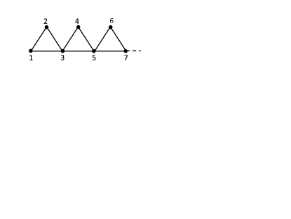
Figure 1: The $\triangle$-chain model.

The ground state of the isotropic Heisenberg model ($\Delta_{1}=$ $\Delta_{2}=1$) with both antiferromagnetic interactions ($J_{1}$, $J_{2}>0$) (AF-delta-chain) has been studied as a function of parameter $\frac{J_{2}}{J_{1}}$ Sen ; Nakamura ; Blundell . Remarkably, for a special choice of the interaction values $J_{1}=2J_{2}$ the lower one-magnon band is dispersionless and the excitations in this band are localized states. The localized nature of the one- magnon states is a base for the construction of multi-magnon states because a state consisting of $k$ independent (non-overlapping) localized magnons is an exact eigenstate. Such construction is possible up to $k\leq\frac{N}{4}$ and these states form the ground state manifold at the saturation magnetic field. The ground state and low-temperature properties of the AF delta-chain with $J_{1}=2J_{2}$ have been studied in detail in Refs.Zhit ; Schmidt ; Derzhko2004 ; Honecker . Typical features related to the localized magnon states are the zero-temperature magnetization plateau and the magnetization jump, residual entropy and extra low-temperature peak in the specific heat.

In contrast to the AF delta-chain the same model with $J_{1}<0$ and $J_{2}>0$ (F-AF delta-chain) is less studied though this model is used as a model of several compounds such as $[Cu(bpy)H_{2}O]\times[Cu(bpy)(mal)H_{2}O](ClO_{4})_{2}$ containing magnetic $Cu^{2+}$ ions Inagaki ; Tonegawa ; ruiz ; Kaburagi . Similarly to the AF delta-chain in this model the localized states exist if $\left|J_{1}\right|=2J_{2}$. It is known Tonegawa that the ground state of the F-AF isotropic delta chain is ferromagnetic for $\alpha=\frac{J_{2}}{\left|J_{1}\right|}<\frac{1}{2}$. In Ref.Tonegawa it was argued that the ground state for $\alpha>\frac{1}{2}$ is a special ferrimagnetic state. The critical point $\alpha=\frac{1}{2}$ is the transition point between these two ground state phases. The isotropic F-AF delta-chain at the transition point $\alpha=\frac{1}{2}$ has been studied in Ref.KDNDR . It was shown KDNDR that in addition to the multi-magnon configurations consisting of isolated magnons the special states with overlapping magnons (localized multi-magnon complex) exist and all of them are exact ground states at zero magnetic field. So, the ground state degeneracy in this model is even larger than for the AF delta-chain. Another difference between two isotropic models concerns the energy gaps between the ground state and the excited states. In the AF delta chain these gaps are finite while in the F-AF model the gaps for $k$-magnon states decrease rapidly with the increase of $k$. As a result the contribution of the excited states to the thermodynamics can not be neglected.

It is interesting to study the influence of the anisotropy of exchange interactions in the F-AF delta-chain on the ground state properties and on the low-temperature thermodynamics. As it will be shown there is a special line in ($\Delta_{1}$,$\Delta_{2}$) plane on which the localized magnons are exact ground states in zero magnetic field. The main aim of this paper is to study the F-AF delta-chain on this line. We will demonstrate that the behavior of the model on this line has non-trivial peculiarities

The paper is organized as follows. In Section II we derive the conditions on model parameters that provides localized magnon eigenstates and, therefore, macroscopic degeneracy of the ground state, which is calculated in Section III. In Section IV we study the low-temperature thermodynamic of the system both analytically and numerically. In Section V we give a summary of our results.

II One-magnon states

We begin the study of the anisotropic F-AF chain described by Eq.(1) with the one-magnon spectrum over ferromagnetic state. Two branches of states with $S^{z}=S_{\max}^{z}-1$ are given by

$$E_{\pm}(q)=\Delta_{1}-\frac{1}{2}\left[\alpha(\Delta_{2}-\cos q)\pm\sqrt{\alpha^{2}(\Delta_{2}-\cos q)^{2}+2(1+\cos q)}\right]$$ (2)

here and further we put $J_{1}=-1$.

At a definite value of $\alpha=\alpha_{0}$ with:

$$\alpha_{0}=\frac{1}{\sqrt{2(1+\Delta_{2})}}$$ (3)

the lower band becomes dispersionless with the energy

$$\varepsilon=\Delta_{1}-\frac{1}{2\alpha_{0}}$$ (4)

We note that the value of $\alpha_{0}$ does not depend on $\Delta_{1}$ but the energy $\varepsilon$ does. The dispersionless one-magnon states correspond to localized states which can be chosen as

$$\hat{\varphi}_{i}\left|F\right\rangle=(s_{2i}^{-}+\frac{1}{\alpha_{0}}s_{2i+1}^{-}+s_{2i+2}^{-})\left|F\right\rangle\quad i=1,\ldots n$$ (5)

where $\left|F\right\rangle$ is the ferromagnetic state with all spins up, $s_{i}^{-}$ is on-site spin lowering operator and $n=N/2$.

The wave function $\hat{\varphi}_{i}\left|F\right\rangle$ is localized in a valley between $i$-th and ($i+1$)-th triangles. The wave functions Eq.(5) are eigenfunctions of $\hat{H}$ at $\alpha=\alpha_{0}$. To prove it let us represent the Hamiltonian $\hat{H}$ as a sum of local Hamiltonians

$$\hat{H}=\sum_{i}\hat{H}_{i}$$ (6)

where $\hat{H}_{i}$ is the Hamiltonian of the $i$-th triangle which is

$$\hat{H}_{i} = -\sum_{\delta=\pm 1}\left(s_{2i+\delta}^{x}s_{2i}^{x}+s_{2i+\delta}^{y}s_{2i}^{y}+\Delta_{1}(s_{2i+\delta}^{z}s_{2i}^{z}-\frac{1}{4})\right)$$ (7)

$$+\alpha\left(s_{2i-1}^{x}s_{2i+1}^{x}+s_{2i-1}^{y}s_{2i+1}^{y}+\Delta_{2}(s_{2i-1}^{z}s_{2i+1}^{z}-\frac{1}{4})\right)$$

It is easy to check that at $\alpha=\alpha_{0}$

$$(\hat{H}_{i}+\hat{H}_{i+1})\hat{\varphi}_{i}\left|F\right\rangle=\varepsilon\hat{\varphi}_{i}\left|F\right\rangle$$ (8)

and $\hat{H}_{j}\hat{\varphi}_{i}\left|F\right\rangle=0$ for $j\neq i,i+1$.

Therefore,

$$\hat{H}\hat{\varphi}_{i}\left|F\right\rangle=\varepsilon\hat{\varphi}_{i}\left|F\right\rangle$$ (9)

Because the one-magnon wave function Eq.(5) is localized it is possible to construct the states with $k$ independent (non-overlapping) localized magnons for $k\leq\frac{N}{4}$ with the energy $E_{k}=\varepsilon k$.

Thus we found that model Eq.(1) for definite choice of parameter $\alpha=\alpha_{0}$ given by Eq.(3) has localized magnon eigenstates Eq.(5) with the energy $\varepsilon$ Eq.(4). If parameters $\Delta_{1}$ and $\Delta_{2}$ are chosen so that $\varepsilon<0$ ($\Delta_{2}>2\Delta_{1}^{2}-1$), all the states composed of $k\leq\frac{N}{4}$ independent localized magnons are the lowest ones in the corresponding spin sector $S^{z}=\frac{N}{2}-k$. It turns out that the lowest state in the case $\varepsilon<0$ lies in the sector $S^{z}=0$ Derzhko2008 . The magnetic properties of the F-AF delta-chain at $\alpha=\alpha_{0}$ and $\varepsilon<0$ are similar to those for the AF isotropic delta-chain with $J_{1}=2J_{2}$. In particular, the ground state magnetization curve has the plateau and the jump, and all the states composed of independent localized magnons form the macroscopically degenerated ground state at the saturation magnetic field.

If $\varepsilon>0$ ($\Delta_{2}<2\Delta_{1}^{2}-1$) the localized magnons are exact eigenstates as well, but they are not the lowest eigenstates. Moreover, if $\varepsilon>0$ the ground state is ferromagnetic with $S_{total}^{z}=\pm\frac{N}{2}$. To prove it let us consider eigenvalues of the triangle Hamiltonian with $\alpha=\alpha_{0}$. The spectrum of each local $\hat{H}_{i}$ consists of four levels, all of them are two-fold degenerated over $S_{z}$:

$$E_{1} = 0,\quad S_{z}=\pm\frac{3}{2}$$

$$E_{2} = \frac{\varepsilon}{2},\quad S_{z}=\pm\frac{1}{2}$$

$$E_{3,4} = \frac{1}{2}(\alpha_{0}+\frac{3\varepsilon}{2}+\frac{1}{2\alpha_{0}})\pm\frac{1}{2}\sqrt{(\alpha_{0}+\frac{\varepsilon}{2}+\frac{1}{2\alpha_{0}})^{2}-2\alpha_{0}\varepsilon},\quad S_{z}=\pm\frac{1}{2}$$ (10)

It follows from Eq.(10) that all eigenvalues for $S_{z}=\pm\frac{1}{2}$ in Eq.(10) are positive at $\varepsilon>0$. Since the local Hamiltonians of neighbor triangles do not commute with each other the ground state energy $E_{0}$ of $\hat{H}$ satisfies an inequality

$$E_{0}\geq\sum_{i}E_{0i}=0$$ (11)

where $E_{0i}=0$ is the ground state energy of $i$-th triangle with $S_{z}=\pm\frac{3}{2}$. The inequality (11) turns in an equality only if all triangles have $S_{z}=\frac{3}{2}$ or $S_{z}=-\frac{3}{2}$ simultaneously. Then, the states with $S_{total}^{z}=\pm\frac{N}{2}$ are two ground states only.

Thus, we conclude that the ground state with $S_{total}^{z}=0$ is realized if $\varepsilon<0$ while for $\varepsilon>0$ the ground state is ferromagnetic. However, if $\varepsilon=0$ the lowest eigenvalues with $S_{z}=\pm\frac{1}{2}$ of the local Hamiltonian becomes zero and it indicates the possibility of a significant increase of the ground state degeneracy.

The condition $\varepsilon=0$ means that model parameters $\Delta_{1}$ and $\Delta_{2}$ are coupled and we parameterize them by the anisotropy of the basal-apical interaction $\Delta_{1}$:

$$\Delta_{2}=2\Delta_{1}^{2}-1$$ (12)

Hamiltonian (1) of the anisotropic F-AF delta-chain with this choice and at $\alpha=\alpha_{0}$ has a form

$$H = -\sum\left(s_{i}^{x}s_{i+1}^{x}+s_{i}^{y}s_{i+1}^{y}+\Delta_{1}\left(s_{i}^{z}s_{i+1}^{z}-\frac{1}{4}\right)\right)$$ (13)

$$+\frac{1}{2\Delta_{1}}\sum\left(s_{2i-1}^{x}s_{2i+1}^{x}+s_{2i-1}^{y}s_{2i+1}^{y}+(2\Delta_{1}^{2}-1)\left(s_{2i-1}^{z}s_{2i+1}^{z}-\frac{1}{4}\right)\right)$$

Model (13) is the main object of the following study. It has macroscopic degeneracy of the ground state and nontrivial thermodynamic properties. When the parameter $\Delta_{1}$ is changed from $\Delta_{1}=0$ to $\Delta_{1}=\infty$ the model interpolates between the isotropic ferromagnetic chain on the basal sites and the Ising model with equal but opposite in sign basal-apical and basal-basal interactions. In the case $\Delta_{1}=1$ model (13) reduces to the isotropic F-AF delta-chain studied in Ref.KDNDR .

As noted in Ref.KDNDR ; Tonegawa , Hamiltonian (13) with $\Delta_{1}=1$ describes the model at the transition point between the ferromagnetic and the ferrimagnetic ground states. In this respect model (13) as a function of $\Delta_{1}$ describes the transition line of more general model, where the parameter $\alpha$ is not put as $\alpha=\frac{1}{2\Delta_{1}}$. This model reads:

$$H = -\sum\left(s_{i}^{x}s_{i+1}^{x}+s_{i}^{y}s_{i+1}^{y}+\Delta_{1}\left(s_{i}^{z}s_{i+1}^{z}-\frac{1}{4}\right)\right)$$ (14)

$$+\alpha\sum\left(s_{2i-1}^{x}s_{2i+1}^{x}+s_{2i-1}^{y}s_{2i+1}^{y}+(2\Delta_{1}^{2}-1)\left(s_{2i-1}^{z}s_{2i+1}^{z}-\frac{1}{4}\right)\right)$$

The ground state phase diagram of model (14) in ($\Delta_{1},\alpha$) plane obtained by numerical calculations is shown in Fig.2. The curve $\alpha=\frac{1}{2\Delta_{1}}$ corresponds to the transition line between different phases shown in Fig.2. We note that the study of the behavior of the model in these phases is out of scope of the present paper and will be given elsewhere. Here we focus on Hamiltonian (13).

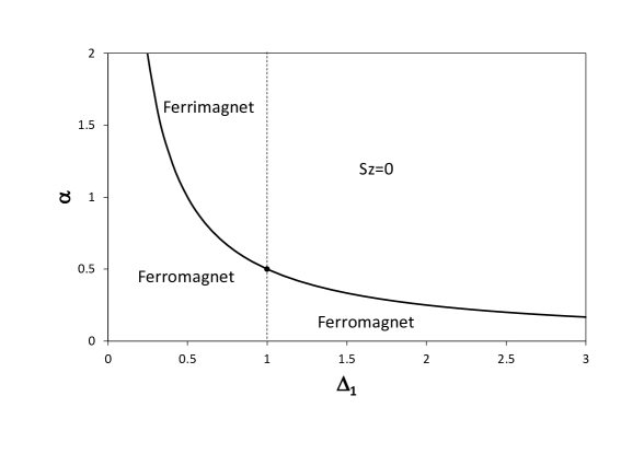
Figure 2: The ground state phase diagram of model (14).

III The ground state degeneracy

In this Section we study the ground state of Hamiltonian (13).

As follows from Eq.(11) the ground state energy of this Hamiltonian is zero. There are $n$ one-magnon states Eq.(5) in the spin sector $S_{total}^{z}=\frac{N}{2}-1$. These states form a complete nonorthogonal basis, have zero energy and, therefore, belong to the ground state manifold.

It is evident that the pairs of the isolated magnons $\varphi_{i}\varphi_{j}$ ($\left|i-j\right|>1$) are the eigenfunctions with zero energy of each local Hamiltonian (and, therefore, of total Hamiltonian) in the spin sector $S_{total}^{z}=\frac{N}{2}-2$. Similarly, eigenfunction composed of $k$ isolated magnons is the exact eigenfunction of the ground state in the sector $S_{total}^{z}=\frac{N}{2}-k$. However, such set of functions contains not all of the states with zero energy in $k$-magnon sector with $k>1$. As it was shown in Ref.KDNDR for the isotropic F-AF delta-chain ($\Delta_{1}=1$) there are also the ground state eigenfunctions of another type, and this type of functions holds in model (13) with $0<\Delta_{1}<\infty$ as well. As an example, we consider two-magnon eigenstates. For $k=2$ along with the pair of isolated magnons we can write the exact two-magnon state as

$$\hat{\varphi}_{i}(\hat{\varphi}_{i-1}+B\hat{\varphi}_{i}+\hat{\varphi}_{i+1})\left|F\right\rangle$$ (15)

where $B=$ $2\Delta_{1}^{2}-1$.

It is easy to check that function (15) is the exact eigenfunction with zero energy for the local Hamiltonians $\hat{H}_{i}$, $\hat{H}_{i+1}$ and $\hat{H}_{i-1}$ and for the others ones. For $\Delta_{1}=1$ this function reduces to that considered in Ref.KDNDR . We note that the function (15) contains overlapping magnons. The complete manifold of ground states in the sector $S_{total}^{z}=\frac{N}{2}-2$ consists of $\frac{n(n-3)}{2}$ pairs ($n=N/2$ is assumed to be even) of independent magnons and $n$ eigenfunctions (15). Thus, the ground state degeneracy in this spin sector is $C_{n}^{2}$.

The construction of the wave functions of type Eq.(15) can be extended for $k>2$. According to the results of Ref.KDNDR the total number of the ground states of the isotropic F-AF chain for fixed $S_{total}^{z}=(n-k)$ ($0\leq k\leq n$) is

$$G_{n}(k) = C_{n}^{k},\qquad 0\leq k\leq\frac{n}{2}$$

$$G_{n}(k) = C_{n}^{n/2}+\delta_{k,n},\qquad\frac{n}{2}\leq k\leq n$$ (16)

The total degeneracy of the ground state $W$ is

$$W = 2^{n}+nC_{n}^{n/2}+1$$ (17)

so that $W=2^{n}\sqrt{\frac{2n}{\pi}}$ in the limit $N\to\infty$.

The analysis similar to that for the isotropic model can be carried out for the anisotropic delta-chain Eq.(13). It turns out that the degeneracy of the ground state given by Eqs.(16)-(17) is valid for all $0<\Delta_{1}<\infty$ except two special cases $\Delta_{1}=1/\sqrt{2}$ and $\Delta_{1}=1/2$ which are considered below.

In the case $\Delta_{1}=1/\sqrt{2}$ the anisotropy $\Delta_{2}$ vanishes and the model reduces to

$$H=-\sum\left(s_{i}^{x}s_{i+1}^{x}+s_{i}^{y}s_{i+1}^{y}+\frac{1}{\sqrt{2}}s_{i}^{z}s_{i+1}^{z}\right)+\frac{1}{\sqrt{2}}\sum\left(s_{2i-1}^{x}s_{2i+1}^{x}+s_{2i-1}^{y}s_{2i+1}^{y}\right)$$ (18)

In this special case the states containing neighbor localized magnons like $\hat{\varphi}_{i}\hat{\varphi}_{i+1}$ are exact ground states ($B=0$ in Eq.(15)), which is not valid in general case. We note that similar type of exact eigenstates arises in the Hubbard model on the delta-chain in which neighboring valleys can be occupied by the localized electrons with identical spins hub1 ; hub2 . The presence of such exact states for model Eq.(18) leads to the increase of the ground state degeneracy, which is

$$W=2^{n}\left(\frac{n}{2}+1\right),\qquad\Delta_{1}=\frac{1}{\sqrt{2}}$$ (19)

In the case $\Delta_{1}=1/2$ after rotation in the XY plane $s_{m}^{x,y}\to(-1)^{m}s_{m}^{x,y}$ the Hamiltonian takes the form

$$H=\sum\left(s_{i}^{x}s_{i+1}^{x}+s_{i}^{y}s_{i+1}^{y}-\frac{1}{2}s_{i}^{z}s_{i+1}^{z}\right)+\sum\left(s_{2i-1}^{x}s_{2i+1}^{x}+s_{2i-1}^{y}s_{2i+1}^{y}-\frac{1}{2}s_{2i-1}^{z}s_{2i+1}^{z}\right)$$ (20)

That is basal-apical and basal-basal interactions are exactly equal in this case. This fact raises symmetry of the system: isosceles triangles in general case becomes equilateral triangles in this special case. The increased symmetry results in the additional degeneracy of the ground state, which is

$$W=2^{n}\left(\frac{n}{3}+1\right)+\frac{2n}{3}+1,\qquad\Delta_{1}=\frac{1}{2}$$ (21)

In the limit $\Delta_{1}=0$ the model reduces to the quantum ferromagnet on basal spins and independent $n$ apical spins. Therefore, the ground state degeneracy is

$$W=\left(n+1\right)2^{n},\qquad\Delta_{1}=0$$ (22)

where the factor $(n+1)$ comes from the degeneracy of the ferromagnetic state over total $S^{z}$.

The special case $\Delta_{1}\to\infty$ will be studied in detail in Sec.IV. Here we give only the results for the ground state degeneracy: $W=3^{n}+1$.

It is interesting to note that the ground state degeneracy of the anisotropic delta-chain with the open boundary conditions (OBC) is the same as for the isotropic model for all value of $0<\Delta_{1}<\infty$. According to the results of Ref.KDNDR the ground state degeneracy of the open chains with add $N$ sites is

$$W_{OBC}=2^{n-1}(n+1),\qquad n=\frac{N+1}{2}$$ (23)

All the above presented expressions for the ground state degeneracy have been confirmed by exact diagonalization (ED) calculations of finite chains.

The exponential degeneracy of the ground state results in the residual entropy $s_{0}=\ln(W)/N$. Though the numbers of degenerated states in the general case Eq.(17) and in special cases Eqs.(19),(21),(22),(23) are different, they yield the same result for the residual entropy in the thermodynamic limit $N\to\infty$:

$$s_{0}=\frac{1}{2}\ln 2$$ (24)

The difference in the numbers of degenerated ground states reveals itself in the corrections $\sim\ln(N)/N$, that vanishes in the thermodynamic limit.

IV Low-temperature thermodynamics

IV.1 Ising model

In this Section we study the low-temperature behavior of the anisotropic F-AF delta-chain on the transition line. We begin with a limit $\Delta_{1}\to\infty$ when model (13) reduces to the Ising model, the Hamiltonian of which has a form:

$$\hat{H}_{I}=-\sum_{i}(s_{i}^{z}s_{i+1}^{z}-\frac{1}{4})+\sum_{i}(s_{2i-1}^{z}s_{2i+1}^{z}-\frac{1}{4})-h\sum_{i}s_{i}^{z}$$ (25)

where we introduced the dimensionless magnetic field $h$.

The partition function of this model can be obtained using a transfer-matrix method and given by

$$Z=\lambda_{1}^{n}+\lambda_{2}^{n}$$ (26)

where eigenvalues of the transfer-matrix are

$$\lambda_{1} = 1+2\cosh\left(\frac{h}{T}\right)+\exp\left(-\frac{1}{T}\right)$$

$$\lambda_{2} = -1+\exp\left(-\frac{1}{T}\right)\quad$$ (27)

The ground state of model (25) at $h=0$ has zero energy and the ground state degeneracy $G_{n}(k)$ in the spin sector $S_{total}^{z}=(n-k)$ ($0\leq k\leq n$) can be found as coefficients in the expansion of $Z$ in powers of $\exp(-h/T)$. As a result $G_{n}(k)$ is given by

$$G_{n}(k)=\sum_{m=0}^{k}C_{n}^{m+n-k}C_{m+n-k}^{m/2}+\delta_{k,n}$$ (28)

The total ground state degeneracy is

$$W=2\sum_{k=0}^{n-1}G_{n}(k)+G_{n}(n)=3^{n}+1$$ (29)

The residual entropy per site $s_{0}$ of the Ising model (25) at $N\to\infty$ equals

$$s_{0}=\frac{1}{2}\ln 3$$ (30)

Using Eqs.(26) and (27) we can obtain all thermodynamic quantities (in the thermodynamic limit only largest eigenvalue $\lambda_{1}$ survives). In particular, the specific heat per site is given by

$$C=\frac{3}{2T^{2}\left[3\exp\left(\frac{1}{2T}\right)+\exp(-\frac{1}{2T})\right]^{2}}$$ (31)

The specific heat as a function of temperature has a typical broad maximum around $T\simeq 0.5$ and exponential decay for $T\to 0$. The zero-field susceptibility per site $\chi$ is given by

$$\chi=\frac{1}{T\left[3+\exp\left(-\frac{1}{T}\right)\right]}$$ (32)

and it behaves as $\chi\sim\frac{1}{3T}$ for $T\to 0$.

Now let us consider the generalization of the Ising model (25) where basal-apical and basal-basal interactions are different:

$$\hat{H}_{I}=-\sum_{i}(s_{i}^{z}s_{i+1}^{z}-\frac{1}{4})+(1+\gamma)\sum_{i}(s_{2i-1}^{z}s_{2i+1}^{z}-\frac{1}{4})-h\sum_{i}s_{i}^{z}$$ (33)

The ground state of model (33) is ferromagnetic for $\gamma<0$ and the ‘antiferromagnetic’ with $S^{z}=0$ on the basal subsystem for $\gamma>0$. The Ising model (25) ($\gamma=0$) describes the transition point between these phases. Generally speaking, the Ising model (33) with $\gamma\neq 0$ is not any limiting case of the initial model (13). Nevertheless, it is useful to study model (33) with $\gamma>0$ because on the one hand it has exact solution and on the other hand some properties of the thermodynamics in the AF phase, especially in the vicinity of the transition point, are inherent in model (13) as well.

The eigenvalues of the transfer-matrix are

$$\lambda_{1,2}=\cosh\left(\frac{h}{T}\right)+\exp\left(-\frac{1}{T}\right)\pm\sqrt{\left[1+\cosh\left(\frac{h}{T}\right)\right]\left[2\exp\left(\frac{\gamma}{T}\right)+\cosh\left(\frac{h}{T}\right)-1\right]}$$ (34)

The partition function at $N\gg 1$ is

$$Z=2^{n}\exp\left(\frac{\gamma n}{2T}\right)\left[1+\frac{1}{2}\exp\left(-\frac{\gamma}{2T}\right)+\frac{1}{2}\exp\left(-\frac{2+\gamma}{2T}\right)\right]^{n}$$ (35)

The ground state degeneracy $W=3^{n}$ for $\gamma=0$ is partially lifted up to $2^{n}$ for $\gamma>0$. The degeneracy $2^{n}$ is related to an independence of the ground state energy for $\gamma>0$ on the spin configuration of the apical subsystem.

The temperature dependence of the specific heat obtained from Eq.(35) has a form

$$C(T)=\frac{(2+\gamma)^{2}\exp\left(-\frac{2+\gamma}{2T}\right)+\gamma^{2}\exp\left(-\frac{\gamma}{2T}\right)+2\exp\left(-\frac{1+\gamma}{T}\right)}{4T^{2}\left[1+2\exp\left(-\frac{\gamma}{2T}\right)+\exp\left(-\frac{2+\gamma}{2T}\right)\right]^{2}}$$ (36)

The specific heat as a function of $T$ is shown in Fig.3 for $\gamma=0.001$. In comparison with the case $\gamma=0$ the dependence $C(T)$ has an additional low-temperature maximum at $T\simeq\frac{\gamma}{4}$. Such two-peak form of the temperature dependence of the specific heat can be explained as follows. The spectrum of the Ising model (33) with $0<\gamma\ll 1$ has two energy scales. One of them is set by ($4^{n}-3^{n}$) states with energies $E\sim 1$ and another one is set by ($3^{n}-2^{n}$) low-energy states that split-off from the ground state at small $\gamma$. According to Eq.(35) the density of the low-energy states having the energy $E=k\gamma/2$ is $\rho(k)=2^{n-k}C_{n}^{k}$ with a maximum at $k=\frac{n}{3}$. This part of the energy spectrum is responsible for the appearance of the low-temperature maximum in $C(T)$. The two-scale form of the low-energy spectrum causes the peculiarities of the other thermodynamic quantities. For example, the entropy per site $s(T)$ has stair-step-like temperature dependence (see Fig.3). In the regions $T\ll\gamma$, $\gamma\ll T\ll 1$, $1\ll T$ the entropy per site $s(T)$ behaves as $s\simeq\frac{1}{2}\ln 2$, $s\simeq\frac{1}{2}\ln 3$, $s\simeq\frac{1}{2}\ln 4$, correspondingly. The quantity $\chi T$ has similar stair-step-likes behavior.

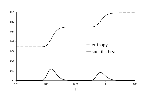
Figure 3: The specific heat and entropy as the function of $T$ of model (33) for $\gamma=0.001$.

IV.2 F-AF delta-chain with $\Delta_{1}\gg 1$

When the parameter $\Delta_{1}$ is large it is convenient to normalize Hamiltonian (13) as $\hat{H}/\Delta_{1}$ and to write it in the form

$$\frac{1}{\Delta_{1}}\hat{H}=\hat{H}_{I}+\hat{V}_{1}+\hat{V}_{2}$$ (37)

where $\hat{H}_{I}$ is the Ising Hamiltonian (25) at $h=0$ and $\hat{V}_{1}$ and $\hat{V}_{2}$ have the forms

$$\hat{V}_{1} = -2g\sum(s_{i}^{x}s_{i+1}^{x}+s_{i}^{y}s_{i+1}^{y})$$

$$\hat{V}_{2} = 2g^{2}\sum(s_{2i-1}^{x}s_{2i+1}^{x}+s_{2i+1}^{y}s_{2i-1}^{y}-s_{2i-1}^{z}s_{2i+1}^{z}+\frac{1}{4})$$ (38)

with small parameter $g=1/(2\Delta_{1})$.

At $g=0$ the ground state of Hamiltonian (37) is $3^{n}$-fold degenerated and there are ($4^{n}-3^{n}$) states with $E\geq 1$. The terms $\hat{V}_{1}$ and $\hat{V}_{2}$ lift the degeneracy for each spin sector, but partly only: the part of the ground state levels remains degenerated with zero energy (the number of them is given by Eq.(17)) and other ones move up. As a result the ground state degeneracy of model (37) is $W\simeq 2^{n}$ in comparison with $W_{I}=3^{n}$ at $g=0$. At $g\ll 1$ the levels of Hamiltonian (37) which split off from the ground state form a set of low-lying excitations determining the low-temperature thermodynamics.

The calculation of the spectrum of these states is very complicated problem and we begin with the one-magnon subspace $S_{total}^{z}=\frac{N}{2}-1$. In the one-magnon subspace the number of degenerate ground states of model (37) is $n$ for both cases $g=0$ and $g\neq 0$, i.e. the perturbation $\hat{V}=\hat{V}_{1}+\hat{V}_{2}$ does not lift the degeneracy. In the two-magnon sector the ground state degeneracies of $\hat{H}_{I}$ and of $\hat{H}$ are $C_{n+1}^{2}$ and $C_{n}^{2}$, correspondingly. It means that $n$ states split off from the ground state. In fact, these states are two-magnon bound complexes and their energy found in the second order in $g$ is $E=g^{2}$.

The calculation of the PT in $g$ for $k=3$ is rather cumbersome and we give the final result only. The set of $(C_{n}^{3}+n(n-1))$ three-magnon states which are degenerated at $g=0$ splits into three subsets. One of them contains $C_{n}^{3}$ ground states with $E=0$. There are $n(n-2)$ states with $E\sim g^{2}$. These states consist of the two-magnon bound complex and the isolated localized magnon. The third subset represents $n$ three-magnon bound complexes with the energy $E=3g^{4}$.

The analytical computation of the spectrum of low-lying excitations for $k>3$ is complicated problem and our further conclusions are based on numerics. According to numerical data the structure of the spectrum of low-lying $k$-magnon states is similar to that for the case $k=3$. The perturbation $\hat{V}=\hat{V}_{1}+\hat{V}_{2}$ splits the ground state manifold into $k$-subsets: the ground states with the energies $E=0$; $k$-magnon bound complexes with $E\sim g^{2(k-1)}$; the states consisting of $(k-1)$-magnon bound complex and one isolated magnon ($E\sim g^{2(k-2)}$); the states consisting of $(k-2)$-magnon bound complex and two isolated magnons ($E\sim g^{2(k-3)}$); and so on. The highest subset of excitations has the energies $E\sim g^{2}$. Thus, the low-lying excitations in the sector with $S_{total}^{z}=\frac{N}{2}-k$ is distinctly divided into the parts with the energies $E\sim g^{2},$ $E\sim g^{4},\ldots E\sim g^{2(k-1)}$.

Taking into account all states with all possible values of $S_{total}^{z}$, we found that the total spectrum of model (37) can be rank-ordered in powers of small parameter $g^{2}$ and it has a multi-scale structure. The ground state degeneracy is given by Eq.(17). The lowest excited states for finite chain composed of $n$ triangles has the energy $E\sim g^{2n-2}$ and it means that the gap is exponentially small.

The distribution of the energy levels for $N=16$ and $g=0.1$ is shown in Fig.4. As it is seen in Fig.4 the spectrum is distinctly divided into the parts. Each part of the spectrum behaves as $E\sim g^{2k}$ as written in Fig.4. This fact was confirmed numerically by comparison of the energies for $g=0.1$ and $g=0.125$. We note that for $N=16$ and $g=0.1$ the value of the smallest excitation $E\sim g^{14}$ becomes very small ($E\sim 10^{-13}-10^{-14}$) and it is indistinguishable from the ground state, so only the excitations with $E>10^{-12}$ are accessible by the ED calculations and represented in Fig.4.

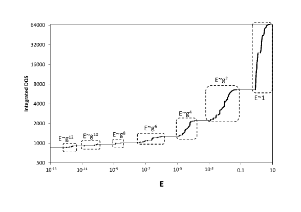
Figure 4: The integrated density of states of normalized Hamiltonian (37) for $g=0.1$ and $N=16$.

Such structure of the spectrum determines the characteristic features of the low-temperature thermodynamics. To study the thermodynamics of model (13) we use the exact diagonalization (ED) of finite delta-chains with PBC up to $N=20$. In Figs.5 and 7 we represent the data for the specific heat $C(T)$ and the entropy $s(T)$ (both per site) for $\Delta_{1}=5$ ($g=0.1$) obtained by the ED for $N=16$ and $N=20$. The temperature dependence of the specific heat shown in Fig.5 exhibits numerous maxima the presence of which can be explained as follows. As it was shown in Sec.IVa the dependence $C(T)$ of the Ising model has one low-temperature maximum which is related to the part of the spectrum with the energy $E\sim\gamma^{2}$. Similarly, multi-scale structure of the spectrum of Eq.(37) for small $g$ leads to the dependence $C(T)$ with many maxima related to the corresponding parts of the spectrum. This is confirmed by the following calculation. Let us select the part of the spectrum with $E\sim g^{2}$, remove the high-energy part with $E\sim 1$, put the energy of all remaining low-lying states to zero (as the ground state) and calculate the contribution of such deformed spectrum to the specific heat. It turns out that this contribution perfectly describes the first low-temperature peak in $C(T)$. Similar procedure for the parts of the spectrum with $E\sim g^{4}$, $E\sim g^{6}$ and so on reproduces very well corresponding peaks in $C(T)$.

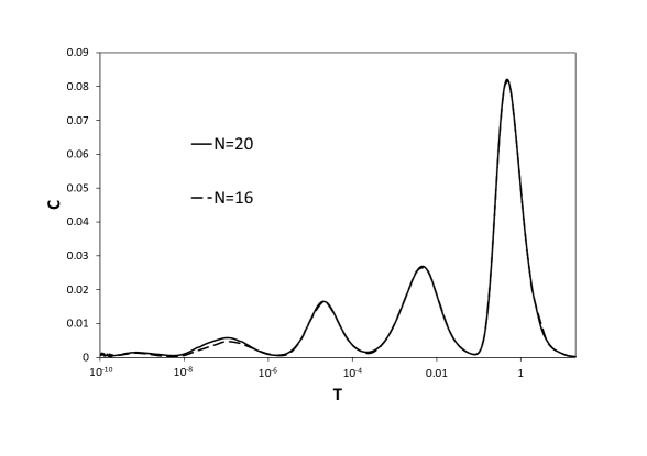
Figure 5: The dependence of specific heat on the temperature of normalized Hamiltonian (37) for $g=0.1$ and $N=16,20$.

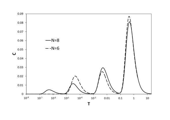
Figure 6: The dependence of specific heat on the temperature of normalized Hamiltonian (37) for $g=0.1$ and $N=6,8$.

The chain consisting of $n$ triangles has $n$ peaks in the dependence $C(T)$. Thus, the number of peaks grows linearly with the system size $N$. It is illustrated in Fig.6, where the specific heat $C(T)$ is shown for $N=6$ and $N=8$ with $g=0.1$. As it can be seen from Fig.6 the number of peaks is three (four) for $N=6(8)$.

Since the $m$-th peak arises from the part of the spectrum with $E\sim g^{2m}$, the maximum of the $m$-th peak takes place at

$$T_{m}\sim\left(cg\right)^{2m}$$ (39)

with some constant $c$.

If the value $g$ is small the corresponding temperature $T_{m}$ is very small as well. For this reason we could not represent in Fig.5 all feasible peaks for $N=16$ and $N=20$ because the temperatures $T_{6}$ and $T_{7}$ for $g=0.1$ are out of the accuracy of the ED calculations.

As it follows from the above the lowest peak should occur at $T_{n}\sim(cg)^{2n}$. This allows us to write the finite-size scaling parameter in the form

$$y=\frac{\ln T}{N\ln g}$$ (40)

The dependence of the entropy per site on temperature for small $g$ has stair-step behavior as shown in Fig.7. These stair steps lie in between the limiting values $s=\ln 2$ for $T\to\infty$ and $s=\frac{1}{2}\ln 2$ for $T\to 0$.

As it can be seen from Figs.5 and 7 the data of $C(T)$ and $s(T)$ for $N=16$ and $N=20$ deviate from each other for $T<T_{0}=10^{-6}$ but they are indistinguishable for $T>T_{0}$. This indicates that the obtained finite-size data correctly describe the thermodynamic limit for temperatures $T>T_{0}$. For example, at least three low-$T$ maxima for $C(T)$ and three stair-steps in the dependence $s(T)$ remain the shape at $N\to\infty$ as in Figs.5 and 7. The levels of the entropy $s(T)$ on these three steps testify that the number of states in sectors is: $4^{n}$ states with $E\sim 1$; $3^{n}$ states with $E\sim g^{2}$; $2.62^{n}$ states with $E\sim g^{4}$; $2.45^{n}$ states with $E\sim g^{6}$.

The deviation of the data for $N=16$ and $N=20$ in the region $T<T_{0}$ means that the finite-size effects become essential for $T<T_{0}$ and the correct description of the thermodynamics in this temperature region needs more large systems. Nevertheless, the multi-scale structure of the spectrum for $\Delta_{1}\gg 1$ will lead certainly to the existence of $n$ maxima in $C(T)$ and $n$ stair-steps in $s(T)$ for chains with $n$ triangles.

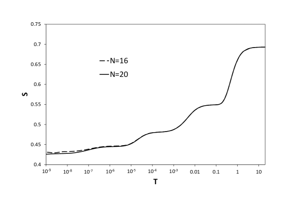
Figure 7: The dependence of entropy on the temperature of normalized Hamiltonian (37) for $g=0.1$ and $N=16,20$.

The temperature dependence of $\chi T$ ($\chi$ is the uniform magnetic susceptibility per spin) has a stair-like behavior similar to the dependence $s(T)$. The numerical data show that the quantity $\chi T$ tends to a finite value depending on $N$ at $T\to 0$ (see Fig.8). This finite value is related to an average of square of $S_{total}^{z}$ over the degenerated ground state as

$$\chi T=\left\langle(S^{z})^{2}\right\rangle_{0}$$ (41)

Evaluating this average with use of Eq.(16) we obtain KDNDR

$$(\chi T)_{n}=\frac{N}{48},\qquad N\to\infty$$ (42)

According to this equation $\chi T$ is proportional to $N$ for $N\gg 1$. It means that $\chi T$ diverges at $T\to 0$ in the thermodynamic limit. The behavior of $\chi T$ for large $N$ and small $T$ depends on the scale variable given by Eq.(40). We will determine the asymptotic behavior of $\chi T$ at $T\to 0$ using the following estimations. We assume that the stair-step-like behavior as in Fig.8 remains in the limit $T\to 0$, so that all steps becomes equal in this limit. Then, for the determination of the low-temperature limit of the susceptibility we need to find the height and width of the steps. According to Eq.(42) the total height is $(\chi T)_{n}=\frac{n}{24}$. This means that each additional triangle in the system leads to the additional stair-step of the height

$$h_{step}=(\chi T)_{n+1}-(\chi T)_{n}=\frac{1}{24}$$ (43)

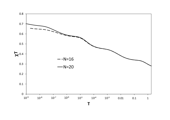
Figure 8: The dependence of magnetic susceptibility on the temperature of normalized Hamiltonian (37) for $g=0.1$ and $N=16,20$.

The width of each stair-step can be estimated as the distance between neighbor peaks in the specific heat, which is

$$w_{step}=\ln\frac{T_{m}}{T_{m+1}}=2\ln\left(cg\right)$$ (44)

The low-temperature limit of the susceptibility can be calculated as envelope of all stair-steps, so that for $\chi T$ we obtain

$$\chi T=\frac{h_{step}}{w_{step}}\ln T$$ (45)

Substituting Eqs.(43) and (44) into Eq.(45) we obtain the low-temperature asymptotic of the susceptibility

$$\chi=\frac{\ln T}{48T\ln\left(cg^{2}\right)}$$ (46)

Susceptibility Eq.(46) can be rewritten in the scaling form which takes into account the finite-size effects:

$$\chi=\frac{N}{48T}f(y)$$ (47)

Here the scaling function $f(y)$ of the scaling variable Eq.(40) has the limits $f(y)=y$ for $y\ll 1$ and $f(\infty)=1$. Thus, in the thermodynamic limit $\chi\sim\ln T/T$ at $T\to 0$.

IV.3 F-AF delta-chain with $\Delta_{1}\ll 1$

In the limit $\Delta_{1}=0$ model (13) reduces to quantum ferromagnet on basal sites and non-interacting apical spins. For $\Delta_{1}\ll 1$ it is convenient to normalize the Hamiltonian (13) in a form

$$\Delta_{1}\hat{H}=\hat{H}_{0}+\hat{V}$$ (48)

where $\hat{H}_{0}$ is the Hamiltonian of the isotropic ferromagnetic basal spin chain and $\hat{V}$ is the basal-apical interaction

$$\hat{H}_{0} = \frac{1}{2}\sum\left(s_{2i-1}^{x}s_{2i+1}^{x}+s_{2i-1}^{y}s_{2i+1}^{y}-s_{2i-1}^{z}s_{2i+1}^{z}+\frac{1}{4}\right)$$

$$\hat{V} = -\Delta_{1}\sum\left(s_{i}^{x}s_{i+1}^{x}+s_{i}^{y}s_{i+1}^{y}\right)+\Delta_{1}^{2}\hat{H}_{I}$$ (49)

The ground state with zero energy of $\hat{H}_{0}$ is $(n+1)$-fold degenerated and all eigenfunctions of $\hat{H}_{0}$ do not depend on the spin state of the apical subsystem. Therefore, the degeneracy of the ground state of model (48) at $\Delta_{1}=0$ in the spin sector $S_{total}^{z}=n-k$ is

$$G_{n}(k)=\sum_{m=0}^{k}C_{n}^{m}$$ (50)

and the total number of the ground states at $\Delta_{1}=0$ is

$$W=2^{n}(n+1)$$ (51)

The perturbation $\hat{V}$ lifts the degeneracy partly and the number of levels which split off from the ground states for fixed $S^{z}$ is $\sum_{m=0}^{k-1}C_{n}^{m}$. These levels form the spectrum of low-energy excitations of Hamiltonian (48) for $\Delta_{1}\ll 1$. In the second order in $\Delta_{1}$ the lowest energy (the gap) in the spin sector $S^{z}=n-k$ for $0\leq k\leq\frac{n}{2}$ is

$$E(k)=\Delta_{1}^{2}(1-\frac{2(k-1)}{n})$$ (52)

For example, the gap for the one-magnon excitations is $E(1)=\Delta_{1}^{2}$. This agrees with the energy of the upper branch of the one-magnon states Eq.(2) at $q=\pi$. As to the gaps in the spin sectors $\frac{n}{2}<k\leq n$, the numerical calculations of finite chains show that they are also proportional to $\Delta_{1}^{2}$. Therefore, the spectrum of model (48) at $\Delta_{1}\ll 1$ has two-scale structure with the energies $E\sim\Delta_{1}^{2}$ and $E\simeq 1$. It is illustrated in Fig.9 where the integrated density of states is shown for $N=16$ and $\Delta_{1}=0.05$. The two-scale spectrum for $\Delta_{1}\ll 1$ is in contrast with the multi-scale spectrum for $\Delta_{1}\geq 1$. Such two-scale structure of the spectrum leads to the temperature dependence of the specific heat with two peaks as shown in Fig.10 for $\Delta_{1}=0.05$. This behavior is in contrast with multi-peaks form of $C(T)$ for $\Delta_{1}\gg 1$.

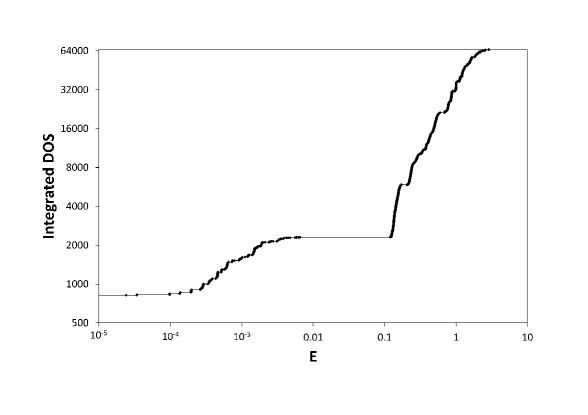
Figure 9: The integrated density of states of normalized Hamiltonian (48) for $\Delta_{1}=0.05$ and $N=16$.

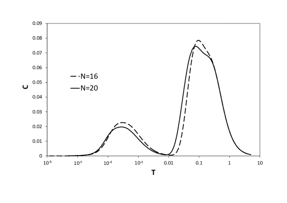
Figure 10: The dependence of specific heat on the temperature of normalized Hamiltonian (48) for $\Delta_{1}=0.05$ and $N=16,20$.

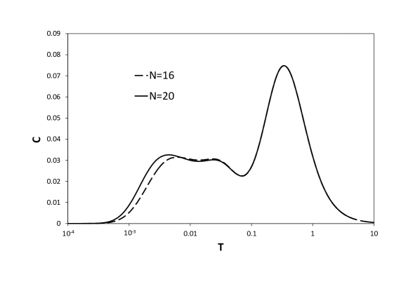
Figure 11: The dependence of specific heat on the temperature of normalized Hamiltonian (48) for $\Delta_{1}=0.5$ and $N=16,20$.

IV.4 F-AF delta-chain with intermediate value of $\Delta_{1}$.

As follows from the results obtained above, the structure of the spectrum of model (13) as well as the low-temperature thermodynamics is qualitatively different in the limiting cases $\Delta_{1}\gg 1$ and $\Delta_{1}\ll 1$. When the parameter $\Delta_{1}$ is neither large nor small the situation is less clear.

Let the parameter $\Delta_{1}$ moves down from the limiting case $\Delta_{1}\gg 1$. Then the ordered partition of the spectrum is smeared and the multi-scale structure of spectrum becomes less obvious. Nevertheless for $\Delta_{1}\geq 1$ the low-temperature behavior of the thermodynamic quantities remains qualitatively similar to that for $\Delta_{1}\gg 1$. For example, the temperature dependence of $C(T)$ for the F-AF delta-chain with $\Delta_{1}=2.5$ and $\Delta_{1}=1$ is shown in Fig.12 and Fig.13. The specific heat is characterized by the existence of the low-T maxima, though they are not so distinctive as in the case $\Delta_{1}=5$ (Fig.5). The reason of this fact is that the finite-size effects become more pronounced when $\Delta_{1}$ decreases. For example, the temperature $T_{0}$ below which the data for $N=16$ and $N=20$ start to deviate from each other is $T_{0}\sim 10^{-6}$, $10^{-4}$, $10^{-3}$ for $\Delta_{1}=5$, $\Delta_{1}=2.5$, $\Delta_{1}=1$, correspondingly. Nevertheless, we expect that the number of low-T peaks of $C(T)$ is proportional to $N$. The behavior of other thermodynamic quantities such as the entropy $s(T)$ and $\chi T(T)$ for $\Delta_{1}=2.5$ and $\Delta_{1}=1$ is qualitatively similar to those for $\Delta_{1}\gg 1$. This suggests that model (13) with $\Delta_{1}\gg 1$ is the generic one for all values of the anisotropy parameter in the range $\Delta_{1}\geq 1$.

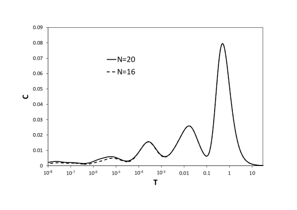
Figure 12: The dependence of specific heat on the temperature of normalized Hamiltonian (37) for $g=0.2$ ($\Delta_{1}=2.5$) and $N=16,20$.

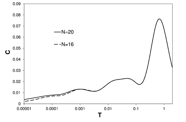
Figure 13: The dependence of specific heat on the temperature for $\Delta_{1}=1$ and $N=16,20$.

However, for $0<\Delta_{1}<1$ the low-T behavior of the thermodynamics changes qualitatively. As it can be seen from Fig.10 and Fig.11 the specific heat $C(T)$ has more complicated form. In addition to the broad maximum at $T\simeq 1$ there is only one (or two) low-T maximum. Unfortunately, the finite-size effects are rather large for $0<\Delta_{1}<1$ and the temperature $T_{0}$ is $T_{0}\simeq 0.01$ and $T_{0}\simeq 0.1$ for $\Delta_{1}=0.5$ and $\Delta_{1}=0.05$. This complicates considerably the determination of the behavior in the thermodynamic limit. All the same, we believe that multi-peak structure for $C(T)$ or many stair-steps one for $s(T)$ does not appear for $0<\Delta_{1}<1$ and the model with $\Delta_{1}\ll 1$ is a generic one in the range $0<\Delta_{1}<1$.

Thus, we suggest that the value $\Delta_{1}=1$ divides the regions of the parameter $\Delta_{1}$ with the qualitatively different behavior of the low-temperature thermodynamics. The possible argument in favor of this assumption is the fact that this model describes the transition line between the ground state phases of different types for $\Delta_{1}\geq 1$ and $\Delta_{1}<1$ (see Fig.2).

V Summary

We have studied the ground state and the low-temperature thermodynamics of the delta-chain with anisotropic F and AF interactions. At definite relations between values of these interactions the lowest branch of the one-magnon states is dispersionless which means the existence of exact localized eigenfunctions. If the energy of the localized states is zero (lowest energy) then they are the ground states. In this case the model depends on a single parameter which can be chosen as the anisotropy of basal-apical spin interaction $\Delta_{1}$. When $\Delta_{1}=\infty$ the model reduces to the Ising model with equal F and AF interactions while for $\Delta_{1}=0$ it is the isotropic ferromagnet on the basal chain and independent spins on the apical sites. Remarkably, the ground state degeneracy is the same for all $0<\Delta_{1}<\infty$ (excluding some special values of $\Delta_{1}$). The degeneracy is macroscopic and leads to finite residual entropy at $T=0$. In the limiting cases $\Delta_{1}=0$ and $\Delta_{1}=\infty$ the ground state degeneracy is even larger and for finite $\Delta_{1}$ it is partially lifted.

For $\Delta_{1}\gg 1$ the excitation spectrum has multi-scale structure and is rank-ordered in powers of small parameter $\Delta_{1}^{-2}$. The number of sections of the spectrum is equal to the number of triangles of the delta-chain and the energy of the levels in the $m$-th section $E\sim\Delta_{1}^{-2m+2}$ ($m=1\ldots N/2$). The origin of such exponentially low energy levels is the fact that the $m$-magnon bound complex in this system has the energy $E_{m}\sim\Delta_{1}^{-2m+2}$. Each $m$-th section of the spectrum is responsible for the appearance of $m$-th peak in the dependence $C(T)$. Thus, the number of the peaks in the specific heat grows with the length of the chain. Similarly, such multi-scale structure of the spectrum determines the characteristic features of the dependence of $s(T)$ and $\chi(T)$. Numerical calculations by the ED of finite delta-chains for smaller values of $\Delta_{1}$ (up to the isotropic point $\Delta_{1}=1)$ show that the behavior of the thermodynamic quantities is qualitatively similar to that for $\Delta_{1}\gg 1$.

For $\Delta_{1}\ll 1$ the spectrum has two-scale structure in contrast with the case $\Delta_{1}\gg 1$. It leads to only one low-temperature maximum in $C(T)$. According to the numerical calculations such feature in the behavior of $C(T)$ survives in the region $\Delta_{1}<1$. Thus, the isotropic point $\Delta_{1}=1$ separates the region of $\Delta_{1}$ on two parts with the qualitatively different behavior of low-temperature thermodynamics. We note that this conclusion is based on numerical calculations and needs more rigorous analysis.

The main points of our study can be extended to delta-chains with arbitrary spin values because the condition on exchange interactions for existence of localized magnons does not depend on the value of spin $s$.

- (1) O. Derzhko, J. Richter, M. Maksymenko, Int. J. Modern Phys. 29, 1530007 (2015).
- (2) C. Wu, D. Bergman, L. Balents, and S. Das Sarma, Phys.Rev.Lett. 99, 070401 (2007).
- (3) Y.-F. Wang, Z.-C. Gu, C.-D. Gong and D.N. Sheng, Phys.Rev.Lett. 107, 146803 (2011).
- (4) K. Sun, Z. Gu, H. Katsura and S. Das Sarma, Phys.Rev.Lett. 106, 236803 (2011).
- (5) J. Richter, O. Derzhko and J. Schulenburg, Phys.Rev.Lett. 93, 107206 (2004).
- (6) M. Maksymenko, A. Honecker, R. Moessner, J. Richter, and O. Derzhko, Phys. Rev. Lett. 109, 096404 (2012).
- (7) M. E. Zhitomirsky and H. Tsunetsugu, Phys.Rev.B 70, 100403 (2004).
- (8) J. Schnack, H.-J. Schmidt, J. Richter and J. Schulenberg, Eur. Phys. J. B 24, 475 (2001).
- (9) J. Richter, J. Schulenburg, A. Honecker, J. Schnack, and H.J. Schmidt, J. Phys.: Condens. Matter 16, S779 (2004).
- (10) O. Derzhko and J. Richter, Phys. Rev. B 70, 104415 (2004).
- (11) M.E. Zhitomirsky and H. Tsunetsugu, Progr. Theor. Phys. Suppl. 160, 361 (2005).
- (12) D. Sen, B.S. Shastry, R.E. Walsteadt and R. Cava, Phys. Rev. B 53 ,6401 (1996).
- (13) T. Nakamura and K. Kubo, Phys. Rev. B 53, 6393 (1996).
- (14) S.A. Blundell and M.D. Nuner-Reguerio, Eur. Phys. J. B 31, 453 (2003).
- (15) Y. Inagaki, Y. Narumi, K. Kindo, H. Kikuchi, T. Kamikawa, T. Kunimoto, S. Okubo, H. Ohta, T. Saito, H. Ohta, T. Saito, M. Azuma, H. Nojiri,, M. Kaburagi and T. Tonegawa, J. Phys. Soc. Jpn. 74, 2831 (2005).
- (16) M. Kaburagi, T. Tonegawa and M. Kang, J.Appl.Phys. 97, 10B306 (2005).
- (17) C. Ruiz-P rez, M. Hern ndez-Molina, P. Lorenzo-Luis, F. Lloret, J. Cano, and M. Julve, Inorg. Chem. 39 3845 (2000).
- (18) T. Tonegawa and M. Kaburagi, J. Magn. Magn. Materials, 272, 898 (2004).
- (19) V. Ya. Krivnov, D. V. Dmitriev, S. Nishimoto S.-L. Drechsler, and J. Richter, Phys. Rev. B 90, 014441 (2014).
- (20) J. Richter, O. Derzhko and A. Honecker, J.Modern Phys. B22, 4418 (2008).
- (21) O. Derzhko, A. Honecker, and J. Richter, Phys. Rev. B 76, 220402 (2007).
- (22) M. Maksymenko, A. Honecker, R. Moessner, J. Richter, and O.Derzhko, Phys. Rev. Lett. 109, 096404 (2012).
- (23) F. Alet et al., J.Phys.Soc.Jpn.Suppl. 74, 30 (2005).