Understanding the dependence on the pulling speed of the unfolding pathway of proteins

Abstract

The dependence of the unfolding pathway of proteins on the pulling speed is investigated. This is done by introducing a simple one-dimensional chain comprising $N$ units, with different characteristic bistable free energies. These units represent either each of the modules in a modular protein or each of the intermediate “unfoldons” in a protein domain, which can be either folded or unfolded. The system is pulled by applying a force to the last unit of the chain, and the units unravel following a preferred sequence. We show that the unfolding sequence strongly depends on the pulling velocity $v_{p}$. In the simplest situation, there appears a critical pulling speed $v_{c}$: for pulling speeds $v_{p}<v_{c}$, the weakest unit unfolds first, whereas for $v_{p}>v_{c}$ it is the pulled unit that unfolds first. By means of a perturbative expansion, we find quite an accurate expression for this critical velocity.

1 Introduction

Since the late twentieth century, research on the mechanical stability of macromolecules turned a prolific field due to the advances in manipulation techniques of individual biomolecules, usually termed single-molecule experiments. One of the most important techniques is atomic force microscopy (AFM), in which a biomolecule is stretched between a rigid platform and the tip of the cantilever [1, 2, 3, 4]. In these experiments, the controlled parameter is either the length of the macromolecule (length-control protocols) or the force exerted over it (force-control protocols), and its conjugated magnitude is measured. As a result, a force-extension curve (FEC) is obtained, which characterizes the elasto-mechanical behaviour of the macromolecule and provides fundamental information about its unfolding pathway [5, 6, 7, 8, 9, 10, 11, 12, 13, 14].

In a typical pulling experiment, the end-to-end distance of the molecule $L$ is increased with a pulling rate $v_{p}$, that is, $dL(t)/dt=v_{p}$. Remarkably, the FEC exhibits a sawtooth pattern [9, 10, 11, 12, 15, 14] showing how the macromolecule comprises several structural units or blocks, in general each one with different stability properties. Each block unfolds individually causing a drop in the measured force. The unfolding pathway is, basically, the order and the way in which the structural blocks of the macromolecule unravel.

Recent studies show that the pulling velocity plays a relevant role in determining the unfolding pathway [14, 16, 17, 18]. Different unfolding pathways are observed depending on (a) which of the ends (C-terminus or N-terminus) the domain is actually pulled from and (b) the pulling speed. It has been claimed that it is the inhomogeneity in the distribution of the force across the protein, for high pulling speeds, that causes the unfolding pathway to change [14, 16, 17, 18]. Nevertheless, to the best of our knowledge, a theory that explains this crossover is still lacking.

We focus on the unfolding pathway of protein domains composed of several stable structural units [16, 17, 19]. In this respect, a good candidate is represented by the Maltose Binding Protein (MBP), a stable and well characterized protein comprising two domains. MBP has been recently employed in studies on mechanical unfolding and translocation [17, 19, 20, 21, 22, 23, 24]. In particular, Bertz and Rief [19] identified four intermediate states in the FEC of mechanical denaturation experiments, each one associated to the unravelling of a specific unit. The authors termed such units “unfoldons” and determined their typical unfolding sequence. However, simulations [17] showed that this unfolding scenario holds only for low pulling speed as the pathway depends on the rate at which the molecule is pulled: at very low pulling rates, it is the weakest unfoldon that unfolds first, while at higher rates the first unfoldon to unravel is the pulled one.

The main purpose of this paper is to develop a physical theory that predicts the observed dependence of the unfolding pathway on the pulling velocity. Specifically, we do so in the adiabatic limit, that is, the regime of slow pulling speeds that allow the system to sweep the whole stationary branches of the FEC [25, 27]. Also, we would like to stress that, although our approach is applied to the unfolding of a single protein, it extends to the unfolding of polyproteins comprising several domains (modular proteins), which unfold sequentially [10].

The plan of the paper is as follows. In section 2, we put forward our model to investigate the unfolding pathway of proteins. In general, the free energy characterizing each unit (unfoldon or module) of the protein is different, that is, there is a certain degree of asymmetry (or disorder) in the free energies. Moreover, we discuss the role of thermal noise and the (ir)relevance of the details of the device controlling the length of the protein. Section 3 is devoted to the analysis of the pulling of the model, by means of a perturbative expansion in both the asymmetry of the free energies and the pulling speed. In sections 3.1 and 3.2 we obtain the corrections introduced by the asymmetry and the finite value of the pulling speed, respectively. In section 3.3 we show that, in the simplest situation, there naturally appears a critical pulling speed $v_{c}$, below (above) which it is the weakest (pulled) unit that unfolds first. In general, when more than one unit has a different free energy, we show that for low (high) enough pulling velocity, it is still the weakest (pulled) unit that unfolds first, but other pathways are present for intermediate velocities. Numerical results for some particular situations are shown in section 4. They are compared to the analytical results previously derived, and a quite good agreement is found. Finally, section 5 deals with the main conclusions of the paper. The appendices cover some technical details that we have omitted in the main text.

2 The model

Let us consider a certain protein domain comprising $N$ unfoldons (or a polyprotein composed of $N$, possibly different, modules). From now on, we will refer to these unfoldons or modules as units. When the molecule is submitted to an external force $F$, the simplest description is to portray it as a one-dimensional chain, where the end-to-end extension of the $i$-th unit in the direction of the force is denoted by $x_{i}$. In a real AFM experiment, the molecule is attached as a whole to the AFM device and stretched. Following Guardiani et al. [17], we model this system with a sequence of nonlinear bonds, as in figure 1: the endpoints of the $i$-th unit are denoted by $q_{i-1}$ and $q_{i}$, so that its extension $x_{i}$ is

$$x_{i}=q_{i}-q_{i-1},\quad i=1,\ldots,N.$$ (1)

The evolution of the system follows the coupled overdamped Langevin equations

$$\gamma\dot{q}_{i}=-\frac{\partial}{\partial q_{i}}G(q_{1},\ldots,q_{N})+\eta_{i},$$ (2)

in which the $\eta_{i}$ are the Gaussian white noise terms, such that $\langle\eta_{i}(t)\rangle=0$ and $\langle\eta_{i}(t)\eta_{j}(t^{\prime})\rangle=2\gamma k_{B}T\delta_{ij}\delta(t-t^{\prime})$, with $\gamma$ and $T$ being the friction coefficient of each unit (the same for all) and the temperature of the fluid in which the protein is immersed, respectively ($k_{B}$ is the Boltzmann constant). The global free energy function of the system is

$$G(q_{1},\ldots,q_{N})=\sum_{i=1}^{N}U_{i}(q_{i}-q_{i-1})+U_{p}(q_{N})\,.$$ (3)

In (3), $U_{p}(q_{N})$ is the contribution to the free energy introduced by the force-control or length-control device (see below), while $U_{i}(x_{i})$ is the single unit contribution to $G$.

The total length of the system is given by

$$\sum_{i=1}^{N}x_{i}=q_{N}.$$ (4)

In force-control experiments, the applied force $F$ is a given function of time, whereas in length-control experiments the device tries to keep the total length $q_{N}$ equal to the desired value $L$, also a certain function of time. The corresponding contributions to the free energy are

$$U_{p}(q_{N})=-Fq_{N},\qquad\text{force-control},$$ (5a)

$$U_{p}(q_{N})=\frac{1}{2}k_{p}(q_{N}-L)^{2},\qquad\text{length-control},$$ (5b)

in which $k_{p}$ stands for the stiffness of the length-control device. The length is perfectly controlled in the limit $k_{p}\to\infty$, when $q_{N}=L$ for all times. A sketch of the model is presented in figure 1.

An apparently similar system, in which each module of the chain follows the Langevin equation $\gamma\dot{x}_{i}=-\partial G/\partial x_{i}+\eta_{i}$ has been recently analyzed [35, 27]. In this approach, the modules are completely independent in force-controlled experiments because these Langevin equations completely neglect the spatial structure of the chain. While this simplifying assumption poses no problem for the characterization of the force-extension curves in [27], it is not suited for the investigation of the unfolding pathway, in which the spatial structure plays an essential role. The spatial structure of biomolecules can be described in quite a realistic way by using a model proposed by Hummer and Szabo several years ago to investigate their stretching [28], but the simplified picture which follows from figure 1 makes an analytical approach feasible.

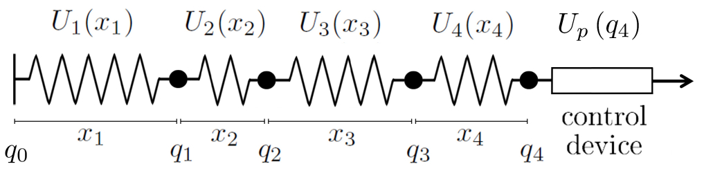
Figure 1: Sketch of the model for a protein with four units. Each unit is represented by a nonlinear spring with potential $U_{i}(x_{i})$, in which $x_{i}$ is the unit’s extension. The beads mark the coordinates $q_{i}$ of their endpoints, so that $x_{i}=q_{i}-q_{i-1}$ (by definition, $q_{0}=0$). Finally, the rectangle stands for the device attached to the pulled end $q_{4}$, which controls either the force applied to the molecule (force-control) or its end-to-end distance (length-control). The contribution of this device to the system’s free energy is $U_{p}(q_{4})$, as shown by (3) and (5).

Now, we turn to look into the unfolding pathway of this system. As the evolution equations are stochastic, this pathway may vary from one trajectory of the dynamics to another. Nevertheless, in many experiments [16, 17, 19] it is observed that there is a quite well-defined pathway, which suggests that thermal fluctuations do not play an important role in determining it. Physically, this means that the free energy barrier separating the unfolded and folded conformations at coexistence (that is, at the critical force, see below) is expected to be much larger than the typical energy $k_{B}T$ for thermal fluctuations. Therefore, we expect the thermal noise terms in our Langevin equations to be negligible and, consequently, they will be dropped in the remainder of the theoretical approach developed in the paper. Of course, if the unfolding barrier for a given biomolecule were only a few $k_{B}T$s, the thermal noise terms in the Langevin equations could not be neglected and our theoretical approach would have to be changed.

In order to undertake a theoretical analysis of the stretching dynamics, one further simplification of the problem will be introduced. We consider that the device controlling the length is perfectly stiff, and the total length $q_{N}=L$ does not fluctuate for all times. We expect this assumption to have little impact on the unfolding pathway: otherwise, the latter would be more a property of the length-control device than of the chain. In fact, we show in section 4 that the unfolding order is not affected by this simplification. For perfect length-control, the mathematical problem is identical to that of the force-control situation, but now the force $F$ is an unknown (Lagrange multiplier) that must be calculated at the end by imposing the constraint $q_{N}=\sum_{i}x_{i}=L$. Therefore, the extensions $x_{i}$’s obey the deterministic equations

$$\gamma\dot{x}_{1}=-U^{\prime}_{1}(x_{1})+U^{\prime}_{2}(x_{2}),$$ (6a)

$$\gamma\dot{x}_{i}=-2U^{\prime}_{i}(x_{i})+U^{\prime}_{i+1}(x_{i+1})+U^{\prime}_{i-1}(x_{i-1}),\quad 1<i<N,$$ (6b)

$$\gamma\dot{x}_{N}=-2U^{\prime}_{N}(x_{N})+U^{\prime}_{N-1}(x_{N-1})+F,$$ (6c)

$$F=\gamma v_{p}+U^{\prime}_{N}(x_{N}).$$ (6d)

We have introduced the pulling speed

$$v_{p}\equiv\dot{L},$$ (7)

which is usually time independent.

We assume that $U_{i}(x_{i})$ allows for bistability in a certain range of the external force $F$, in the sense that $U_{i}(x_{i})$ $-Fx_{i}$ is a double-well potential with two minima, see figure 2. Therefore, in that force range, each unit may be either folded, if $x_{i}$ is in the well corresponding to the minimum with the smallest extension, or unfolded, when $x_{i}$ belongs to the well with the largest extension. If the length is kept constant ($v_{p}=0$), there is an equilibrium solution of (6),

$$U^{\prime}_{1}(x_{1}^{\text{st}})=U^{\prime}_{2}(x_{2}^{\text{st}})=\cdots=U^{\prime}_{N}(x_{N}^{\text{st}})=F^{\text{st}},$$ (8)

and $F^{\text{st}}$ is calculated with the constraint $\sum_{i}x_{i}^{\text{st}}=L$. This solution is stable as long as $U^{\prime\prime}_{i}(x_{i}^{\text{st}})>0$ for all $i$.

If all the units are identical, $U_{i}(x)=U(x)$, the metastability regions of each module (the range of forces for which the equation $U^{\prime}_{i}(x)=F$ has several solutions) coincide. Therefore, we obtain stationary branches corresponding to $J$ unfolded units and $N-J$ folded units that have been analyzed in detail in [25, 27]. If all the modules are not identical, the metastability regions do not perfectly overlap since the units are not equally strong: the weakest one is that for which the equation $U^{\prime}_{i}(x)=F$ ceases to have multiple solutions for a smaller force value.

It is important to note that we can change all the forces $U^{\prime}_{i}(x_{i})$ to $V^{\prime}_{i}(x_{i})=U^{\prime}_{i}(x_{i})-F_{0}$ and $F$ to $\varphi=F-F_{0}$, we have the same system (6) but with $V^{\prime}_{i}$ and $\varphi$ instead of $U^{\prime}_{i}$ and $F$, respectively. Then, we may use the free energies for any common value of the force $F_{0}$ and interpret the Lagrange multiplier as the excess force from this value to be applied to the system.

3 The pulled chain

Let us consider the pulling of our system. We write the $i$-th-unit free energy as

$$U_{i}(x)=U(x)+\xi\,\delta U_{i}(x),$$ (9)

in which $U(x)$ is the “main” part, common to all the units, and $\xi\delta U_{i}(x)$ represents the separation from this main contribution. If all the units are perfectly identical, $U_{i}(x)=U(x)$ for all $i$ or, equivalently, $\delta U_{i}(x)=0$. In principle, in an actual experiment, the splitting of the free energy in (9) can be done if the free energy $U_{i}$ of each unit is known: we may define the common part as the “average” free energy over all the units, $U(x)\equiv\overline{U}(x)\equiv N^{-1}\sum_{i=1}^{N}U_{i}(x)$, and $\xi\delta U_{i}(x)\equiv U_{i}(x)-\overline{U}(x)$. From a physical point of view, the dimensionless parameter $\xi>0$ measures the importance of the heterogeneity in the free energies. Our theory could be applied to a situation in which the free energy deviations $\delta U_{i}$ were stochastic and followed a certain probability distribution, for instance to represent the slight differences among very similar units, as done in [27] to analyze the force-extension curves. In particular, the forces $U^{\prime}_{i}(x)$ in the evolution equations can also be split as

$$U^{\prime}_{i}(x)=U^{\prime}(x)+\xi\,\delta\!f_{i}(x),\quad\delta\!f_{i}(x)\equiv\delta U^{\prime}_{i}(x).$$ (10)

As already noted above, we can use the free energies for any common value of the force $F_{0}$, and interpret $F$ as the extra applied force from this value. In what follows, we consider $U(x)$ with two, equally deep, minima corresponding to the folded (F) and unfolded (U) configurations. Figure 2 presents a qualitative picture of the free energy and its derivative. The two minima correspond to lengths $\ell_{F}$ and $\ell_{U}$, with $\ell_{F}<\ell_{U}$. Also the point $\ell_{b}$ at which $U^{\prime\prime}(\ell_{b})=0$ is marked.

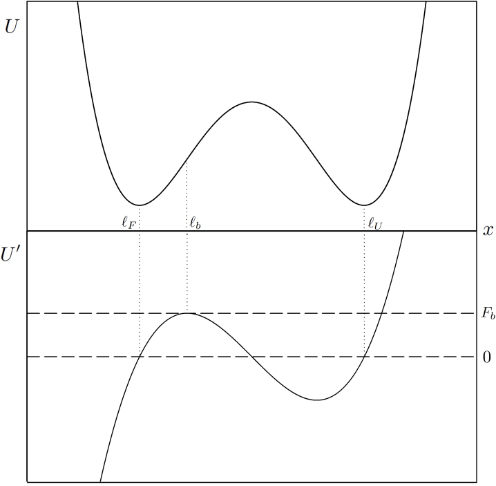
Figure 2: Qualitative behaviour of the main contribution to the free energy $U(x)$ at the critical force (top panel) and associated force $U^{\prime}(x)$ (bottom panel) as a function of the extension. The values of the lengths at the folded and unfolded minima are $\ell_{F}$ and $\ell_{U}$, respectively, whereas the threshold length $\ell_{b}$ stands for the length corresponding to the limit of stability and $F_{b}$ is the corresponding force.

It is the condition $U^{\prime\prime}(\ell_{b})=0$ that essentially determines the stability threshold, as it provides the limit force $F_{b}=U^{\prime}(\ell_{b})>0$ at which the folded basin ceases to exist for the “main” potential. In the deterministic approximation considered here, thermal fluctuations are neglected and, for $F<F_{b}$, the folded unit cannot jump over the free energy barrier hindering its unfolding: it has to wait until, at $F=F_{b}$, the only possible extension is that of the unfolded basin. Of course, neglecting thermal noise restricts in some way the range of applicability of our results, see section 3.3 for a more detailed discussion and also the numerical section 4.

Keeping the above discussion in mind, now we analyze the limit of stability of the different units. The asymmetry correction $\delta f_{i}$ shifts the threshold force for the different units. The extension $x_{i,b}$ at which the $i$-th unit loses its stability is obtained by solving the equation $U^{\prime\prime}_{i}(x_{i,b})=U^{\prime\prime}(x_{i,b})+\xi\delta f^{\prime}_{i}(x_{i,b})=0$, which linearized in both the displacement $x_{i,b}-\ell_{b}$ and $\xi$ reads

$$U^{\prime\prime}(\ell_{b})+U^{\prime\prime\prime}(\ell_{b})(x_{i,b}-\ell_{b})+\xi\delta f^{\prime}_{i}(\ell_{b})=0.$$ (11)

Noting that $U^{\prime\prime}(\ell_{b})=0$, we get that

$$x_{i,b}=\ell_{b}-\xi\,\frac{\delta f^{\prime}_{i}(\ell_{b})}{U^{\prime\prime\prime}(\ell_{b})}.$$ (12)

See A for details. The corresponding force is

$$F_{i,b}=F_{b}+\xi\,\delta\!f_{i}(\ell_{b}),$$ (13)

in which we have also dropped terms of the order of $\xi^{2}$. Then, units with $\delta\!f_{i}(\ell_{b})<0$ ($\delta\!f_{i}(\ell_{b})>0$) are weaker (stronger) than average.

When the system is continuously pulled, the total length of the system $L$ has been shown to be a good reaction coordinate [30]. Therefore, on physical grounds it is reasonable to use $L$ to measure time and write the evolution equations (6) as

$$\gamma v_{p}\frac{dx_{1}}{dL}=-U^{\prime}(x_{1})+U^{\prime}(x_{2})+\xi[-\delta f_{1}(x_{1})+\delta\!f_{2}(x_{2})],$$ (14a)

$$\gamma v_{p}\frac{dx_{i}}{dL}=-2U^{\prime}(x_{i})+U^{\prime}(x_{i+1})+U^{\prime}(x_{i-1})+\xi[-2\delta\!f_{i}(x_{i})+\delta\!f_{i+1}(x_{i+1})+\delta f_{i-1}(x_{i-1})],$$

$$\qquad\qquad\qquad\qquad\qquad\qquad\qquad\qquad\qquad\qquad\qquad 1<i<N,$$ (14b)

$$\gamma v_{p}\frac{dx_{N}}{dL}=-2U^{\prime}(x_{N})+U^{\prime}(x_{N-1})+F+\xi[-2\delta f_{N}(x_{N})+\delta\!f_{N-1}(x_{N-1})],$$ (14c)

$$F=\gamma v_{p}+U^{\prime}(x_{N})+\xi\,\delta\!f_{N}(x_{N}).$$ (14d)

Moreover, this change of variable makes the pulling speed $v_{p}$ appear explicitly in the equations, allowing us to consider $v_{p}$ as a perturbation parameter for slow enough pulling processes.

Now, we consider a system in which the asymmetry in the free energies is small and which is slowly pulled. Thus, (14) is solved by means of a perturbative expansion in powers of the pulling velocity $v_{p}$ and the disorder parameter $\xi$, that is,

$$x_{i}(L)=x_{i}^{(0)}(L)+\xi\delta x_{i}(L)+v_{p}\Delta x_{i}(L),$$ (15a)

$$F(L)=F^{(0)}(L)+\xi\delta F(L)+v_{p}\Delta F(L),$$ (15b)

up to the linear order in both $v_{p}$ and $\xi$.

The zero-th (lowest) order corresponds to the chain of identical units ($\xi=0$) with a given constant length $L$ ($v_{p}=0$). Namely, $x_{i}^{(0)}$ and $F^{(0)}$ obey the equations

$$0=-U^{\prime}(x_{1}^{(0)})+U^{\prime}(x_{2}^{(0)}),$$ (16a)

$$0=-2U^{\prime}(x_{i}^{(0)})+U^{\prime}(x_{i+1}^{(0)})+U^{\prime}(x_{i-1}^{(0)}),\quad 1<i<N,$$ (16b)

$$0=-2U^{\prime}(x_{N}^{(0)})+U^{\prime}(x_{N-1}^{(0)})+F^{(0)},$$ (16c)

$$F^{(0)}=U^{\prime}(x_{N}^{(0)}).$$ (16d)

The solution of this system is straightforward,

$$U^{\prime}(x_{i}^{(0)})=F^{(0)},$$ (17)

the force is equally distributed among all the units of the chain in equilibrium, as expected. If we start the pulling process from a configuration in which all the units are folded and the force is outside the metastability region (the usual situation), the units extensions and the applied force are

$$x_{i}^{(0)}=\ell\equiv\frac{L}{N},\quad\forall i,\qquad F^{(0)}=U^{\prime}(\ell),$$ (18)

to the lowest order. To calculate the linear corrections in $\xi$ and $v_{p}$, we have to substitute (15) and (18) into (14), and equate terms proportional to $\xi$ and $v_{p}$, respectively. This is done below in two separate sections: firstly, for the asymmetry contribution $\delta x_{i}$ and, secondly, for the “kinetic” contribution $\Delta x_{i}$.

3.1 Asymmetry correction

All the modules are not characterized by the same free energy, and here we calculate the first order correction introduced thereby. The asymmetry corrections $\delta x_{i}$ obey the system of equations

$$\delta x_{2}-\delta x_{1}=\frac{\delta\!f_{1}(\ell)-\delta\!f_{2}(\ell)}{U^{\prime\prime}(\ell)},$$ (19a)

$$\delta x_{i+1}+\delta x_{i-1}-2\delta x_{i}=\frac{2\delta\!f_{i}(\ell)-\delta\!f_{i+1}(\ell)-\delta\!f_{i-1}(\ell)}{U^{\prime\prime}(\ell)},\quad 1<i<N$$ (19b)

$$\delta x_{N-1}-2\delta x_{N}=\frac{2\delta\!f_{N}(\ell)-\delta\!f_{N-1}(\ell)-\delta F}{U^{\prime\prime}(\ell)},$$ (19c)

$$\delta F=U^{\prime\prime}(\ell)\delta x_{N}+\delta\!f_{N}(\ell),$$ (19d)

which is linear in the $\delta x_{i}$’s, and thus can be analytically solved. It is clear that our expansion breaks down when $U^{\prime\prime}(\ell)=0$. This was to be expected, since we know that the stationary branch with all the modules folded is unstable when $U^{\prime\prime}_{i}$ becomes negative for some unit $i$, and to the lowest order this takes place when $U^{\prime\prime}(\ell)=0$.

The solution of the above system of difference equations is obtained by standard methods [31], with the result

$$\delta x_{i}=\frac{\overline{\delta\!f}(\ell)-\delta\!f_{i}(\ell)}{U^{\prime\prime}(\ell)},\;\forall i,\quad\delta F=\overline{\delta\!f}(\ell)=\frac{1}{N}\sum_{i=1}^{N}\delta f_{i}(\ell).$$ (20)

See B for more details. Interestingly, the force is homogeneous across the chain, since to first order in $\xi$ we have that

$$U^{\prime}_{i}(x_{i})=U^{\prime}(x_{i}^{(0)})+\xi[U^{\prime\prime}(x_{i}^{(0)})\delta x_{i}+\delta\!f_{i}(x_{i}^{(0)})]=U^{\prime}(\ell)+\xi\overline{\delta\!f}(\ell)=F^{(0)}+\xi\delta F.$$ (21)

This is nothing but the stationary solution (8), up to first order in the disorder. Moreover, (20) implies that there are units with $\delta x_{i}>0$ and others with $\delta x_{i}<0$, depending on the sign of $\overline{\delta\!f}(\ell)-\delta\!f_{i}(\ell)$. This is a consequence of our perturbation expansion, since $\sum_{i}x_{i}^{(0)}=L$ for all times, as given by (18), and thus $\sum_{i}\delta x_{i}=0$.

Let us remember that we denote by $\ell_{b}$ the value of the extension at which the common main free energy reaches its limit of stability, see figure 2. Taking into account only the asymmetry correction, it is the weakest unit that unfolds first, since the most negative $\delta\!f_{i}(\ell)$ leads to the largest positive $\delta x_{i}$ and then it is the one that first verifies the condition $x_{i}=\ell+\xi\delta x_{i}=\ell_{b}$ (for a more detailed discussion, see A). An alternative way of looking at this is to recall that the force corresponding to the limit of stability is smallest for the weakest unit: since the force is homogeneously distributed along the chain, it is the weakest module that first reaches its stability threshold.

3.2 Correction due to the finite pulling speed

Now we look into the “kinetic” correction due to the finite pulling speed $v_{p}$. The zero-th order solution is given by (18), so that $dx_{i}^{(0)}/dL=N^{-1}$ for all $i$, and we have

$$\Delta x_{2}-\Delta x_{1}=\frac{\gamma}{NU^{\prime\prime}(\ell)},$$ (22a)

$$\Delta x_{i+1}+\Delta x_{i-1}-2\Delta x_{i}=\frac{\gamma}{NU^{\prime\prime}(\ell)},\quad 1<i<N,$$ (22b)

$$\Delta x_{N-1}-2\Delta x_{N}=\frac{1}{U^{\prime\prime}(\ell)}\left[\frac{\gamma}{N}-\Delta F\right],$$ (22c)

$$\Delta F=\gamma+U^{\prime\prime}(\ell)\Delta x_{N}.$$ (22d)

The solution to this system of linear difference equations [31] is

$$\Delta x_{i}=\frac{\gamma}{2NU^{\prime\prime}(\ell)}\left[i(i-1)-\frac{(N+1)(N-1)}{3}\right],$$ (23a)

$$\Delta F=\frac{(N+1)(2N+1)\gamma}{6N}.$$ (23b)

See B for more details. Again, $\sum_{i}\Delta x_{i}=0$ because the zero-th order solution (18) gives the total length, $\sum_{i}x_{i}^{(0)}=L$ for all times. (23a) is reasonable on intuitive grounds: the kinetic correction $\Delta x_{i}$ increases with $i$ because the last module is the one that is actually pulled. Therefore, on the basis of only the kinetic correction, it is the last module that would unfold first because $\Delta x_{N}$ is the largest. Thus, the condition $x_{i}=\ell+v_{p}\Delta x_{i}=\ell_{b}$ is first verified for $i=N$.

It is interesting to note that the force was equally distributed for the asymmetry correction, as expressed by (21), but this is no longer true if we incorporate the kinetic correction. Up to the the first order, $U^{\prime}_{i}(x_{i})=U^{\prime}(x_{i}^{(0)}+\xi\delta x_{i}+v_{p}\Delta x_{i})+\xi\delta\!f_{i}(x_{i})\simeq U^{\prime}(\ell)+\xi\overline{\delta\!f}(\ell)+v_{p}U^{\prime\prime}(\ell)\Delta x_{i}$. Therefore, the force $U^{\prime}_{i}(x_{i})$ depends on the unit $i$: for all times, it is smaller the further from the pulled unit we are. Again, there is an alternative way of understanding why the last unit would unfold first if we were considering perfectly identical units ($\xi=0$): for any time, it would be the last unit that suffered the largest force and thus the first that reached their common limit of stability $F_{b}$.

3.3 The critical velocities

If the last unit is not the weakest, there is a competition between the asymmetry and the kinetic corrections. For very low pulling speeds, in the sense that $v_{p}/\xi\to 0$, the term proportional to $v_{p}$ can be neglected and it is the weakest unit (the one with the largest $\delta x_{i}$) that unfolds first, as discussed in section 3.1. On the other hand, for very small disorder, in the sense that $\xi/v_{p}\to 0$, the term proportional to $\xi$ is the one to be neglected and it is the last unit (the one with the largest $\Delta x_{i}$) that unfolds first, as also discussed in section 3.2. Therefore, different unfolding pathways are expected as the pulling speed changes.

Collecting all the contributions to the extensions, we have that

$$x_{i}=\ell+\frac{\xi\overline{\delta\!f}(\ell)-v_{p}\gamma\dfrac{N^{2}-1}{6N}}{U^{\prime\prime}(\ell)}+\frac{v_{p}\gamma\dfrac{i(i-1)}{2N}-\xi\delta\!f_{i}(\ell)}{U^{\prime\prime}(\ell)}.$$ (24)

We have rearranged the terms in $x_{i}$ in such a way that the first two terms on the rhs are independent of the unit $i$, all the dependence of the length of the module on its position across the chain has been included in the last term. Note that we are expanding the solution in powers of $v_{p}$ around the “static” solution, which is obtained by putting $v_{p}=0$ in (24). Thus, the “static” solution corresponds to the stationary one the system would reach if we kept the total length constant and equal to its instantaneous value at the considered time. It is essential to realise that (24) is only valid for very slow pulling, as long as the corrections to the “static” solution are small, and this is the reason why the limit of stability is basically unchanged as compared to the static case. In order to be more precise, we refer to this kind of very slow pulling as adiabatic pulling. A main result of our paper is that, even for the case of adiabatic pulling, there appear different unfolding pathways depending on the value of the pulling speed.

In the adiabatic limit we are considering here, the pulling process has to be slow enough to make the system move very close to the stationary force-length branches, but not so slow that the system has enough time to escape from the folded basin. As discussed in [27], there is an interplay between the pulling velocity and thermal fluctuations. For very slow pulling velocities, the system has enough time to surpass the energy barrier separating the two minima, which leads to the typical logarithmic dependence of the “unfolding force” $F_{U}$ on the pulling speed, specifically $F_{U}\propto(\ln v_{p})^{a}$ [44, 29]. On the other hand, as already argued at the beginning of section 3, for adiabatic pulling, the units unfold not because they are able to surpass the free energy barrier but because the folded state ceases to exist at the force $F_{b}$ corresponding to the upper limit of the metastability region.

The unit that unfolds first is the one for which $x_{i}=\ell_{b}$ for the shortest time. In light of the above, it is natural to investigate whether it is possible to determine which module is the first to unfold for a given pulling speed. To put it another way, we would like to calculate the “critical” velocities which separate the velocity intervals in which a specific module unfolds first. Let us assume that, for a given pulling speed $v_{p}$, it is the $i$-th module that unfolds first. All the modules $j$ to its left, that is, with $j<i$, will not open first if the pulling velocity is further increased because the difference between the kinetic corrections $\Delta x_{i}-\Delta x_{j}$ increases with $v_{p}$. Therefore, the first module $j$ to unfold when the velocity is sufficiently increased it is always to its right. The velocity $v^{i}(j)$ for which each couple of modules $(i,j)$, $j>i$, reach simultaneously the stability threshold is determined by the condition

$$x_{i}(\ell_{c})=x_{j}(\ell_{c})=\ell_{b}$$ (25)

(25) determines both the value of $\ell_{c}$ (or time $t_{c}$) at which the stability threshold is reached and the relationship between $v_{p}$ and $\xi$. (24) implies that

$$-\xi\delta f_{i}(\ell_{c})+\gamma v^{i}(j)\frac{i(i-i)}{2N}=-\xi\delta\!f_{j}(\ell_{c})+\gamma v^{i}(j)\frac{j(j-1)}{2N}.$$ (26)

We already know that the length corresponding to the limit of stability is very close to the threshold length $\ell_{b}$, its distance thereto being of the order of $\sqrt{\xi}$, as shown in A. Therefore, to the lowest order, $\ell_{c}$ can be approximated by $\ell_{b}$, and we get

$$\frac{\gamma v^{i}(j)}{\xi}=\frac{2N[\delta\!f_{j}(\ell_{b})-\delta\!f_{i}(\ell_{b})]}{j(j-1)-i(i-1)},\quad j>i.$$ (27)

Clearly, the minimum of these velocities is the one that matters: Let us denote by $j^{(i)}_{\text{min}}$ the position of the module for which $v^{i}(j)$ reaches its minimum value $v_{\text{min}}^{i}$,

$$v_{\text{min}}^{i}=v^{i}(j^{(i)}_{\text{min}})=\min_{j}v^{i}(j)$$ (28)

for $v_{p}$ just below $v_{\text{min}}^{i}$, it is the $i$-th module that unfolds first, but for $v_{p}$ just above $v_{\text{min}}^{i}$, it is the $j$-th module that unfolds first. Let us denote the weakest module by $\alpha_{1}$, that is, $\delta\!f_{i}(\ell_{b})$ is smallest for $i=\alpha_{1}$. If $v_{p}$ is smaller than $v_{\text{min}}^{\alpha_{1}}$, the first unit to reach the stability limit is the weakest one. Then, we rename the latter velocity $v_{c}^{(1)}$, that is,

$$v_{c}^{(1)}=v_{\text{min}}^{\alpha_{1}},\quad\delta\!f_{\alpha_{1}}(\ell_{b})=\min_{i}\delta\!f_{i}(\ell_{b}),$$ (29)

because it is the first one of a (possible) series of critical velocities separating different unfolding pathways, see below.

Let us denote by $\alpha_{2}$ the module which unfolds first in the “second” velocity region, $v_{p}$ just above $v_{c}^{(1)}$, that is, $\alpha_{2}=j_{\text{min}}^{(\alpha_{1})}$. This unit ceases to be the first to unfold for the velocity

$$v_{c}^{(2)}=v_{\text{min}}^{\alpha_{2}}$$ (30)

The successive changes on the unfolding pathway take place at the critical velocities

$$v_{c}^{(k)}=v_{\min}^{\alpha_{k}},$$ (31)

in which $\alpha_{k+1}=j_{\text{min}}^{(\alpha_{k})}$. This succession ends when $\alpha_{k+1}=N$: in that case, for $v_{p}>v^{(k)}_{c}$, the first unit to unfold is always the pulled one. This upper critical velocity $v_{c}^{\text{end}}$ can be computed in a more direct way,

$$v_{c}^{\text{end}}=\max_{j}v_{\text{min}}^{j}(N).$$ (32)

Consistency of the theory requires that $v_{c}^{(k+1)}>v_{c}^{(k)}$; a short proof is presented in C.

We have a trivial case for $\alpha_{1}=N$, when the pulled unit is precisely the weakest and it is always the first to unfold for any pulling speed. The simplest nontrivial case appears when all the modules has the same free-energy with the exception of the weakest, and $\alpha_{1}\neq N$, (27), (29) and (32) reduce to

$$\frac{\gamma v^{(1)}_{c}}{\xi}=\frac{\gamma v^{\text{end}}_{c}}{\xi}=\frac{2N[\delta\!f_{N}(\ell_{b})-\delta\!f_{\alpha_{1}}(\ell_{b})]}{N(N-1)-\alpha_{1}(\alpha_{1}-1)}.$$ (33)

Note that the situation is quite simple, since there exist a single critical velocity $v_{c}=v_{c}^{(1)}=v_{c}^{\text{end}}$. For $v_{p}<v_{c}$ the weakest module unfolds first whereas for $v_{p}>v_{c}$ the last one unfolds first. In general, when the units have different free energies the situation may be more complex, as shown in the previous paragraph. There appear intermediate critical velocities, which define pulling speed windows where neither the weakest unit nor the last one is the first to unfold. In order to obtain these regions, we need to recursively evaluate (31).

4 Numerical results

Throughout this numerical section, we check the agreement between our theory and the numerical integration of the evolution equations. Firstly, we discuss the validity of the simplifications introduced in the development of the theory, namely (i) negligible thermal noise and (ii) perfect length-control. Secondly, we look into the critical pulling speed, showing that there appears such a critical speed in the simulations and comparing this numerical value to the theory developed before.

We consider a system composed of $N=4$ unfoldons, such as the maltose binding protein [17], each one characterized by a quartic bistable free energy. In reduced variables, the free energies have the form $U_{i}(x)=\epsilon_{i}U(x)$, where

$$U(x)=\frac{1}{4}\left[(x-\sigma)^{2}-a^{2}\right]^{2},$$ (34)

with $\epsilon_{i}=1$ for $i\neq 1$, $\epsilon_{1}<1$, $\sigma=0$ and $a=3$. The value of the friction coefficient is, also in reduced variables, $\gamma=1$. We use these dimensionless reduced variables in order to make it easier to compare our results to those in [17]. The function (34) is one of the simplest, but reasonable, choice to describe the free energy of different unfoldons of the same protein domain. Using our notation, we have

$$\delta\!f_{i}(x)=0,\;i\neq 1,\qquad\delta\!f_{1}(x)=-\xi U^{\prime}(x),$$ (35)

with $\xi=1-\epsilon_{1}$. (12) and (13) give us the limits of stability up to first order in the asymmetry $\xi$,

$$x_{i,b}=\ell_{b},\;\forall i,\quad F_{i,b}=F_{b},\;i\neq 1,\qquad F_{1,b}=(1-\xi_{1})F_{b}.$$ (36)

For this simple example, (36) is exact. The weakest unit is the first one, because $F_{1,b}$ is the minimum value of the force at the limit of stability. For the values of the parameters we are using, $\ell_{b}=a/\sqrt{3}=1.73$ and $F_{b}=U^{\prime}(\ell_{b})=2\sqrt{3}a^{3}/9=10.4$. Since we are writing the free energies for a common given value of the force, we are assuming that all the units have their two minima equally deep at the same force. This assumption is made to keep things simple: the main ingredient for having an unfolding pathway that depends on the pulling speed is to have different values of the forces $F_{i,b}$ at the stability threshold for the different units.

In the case we are considering, the weakest unit is the first one, while the others share the same free energy. This means that we have the simplest scenario for the critical velocity in our theoretical approach: it is always the weakest (for $v_{p}<v_{c}$) or the last (for $v_{p}>v_{c}$) unit that opens first, as discussed at the end of the previous Section. Here, (33) for $\alpha_{1}=1$ and $N=4$ reduces to

$$\frac{\gamma v_{c}}{\xi}=\frac{2}{3}F_{b}.$$ (37)

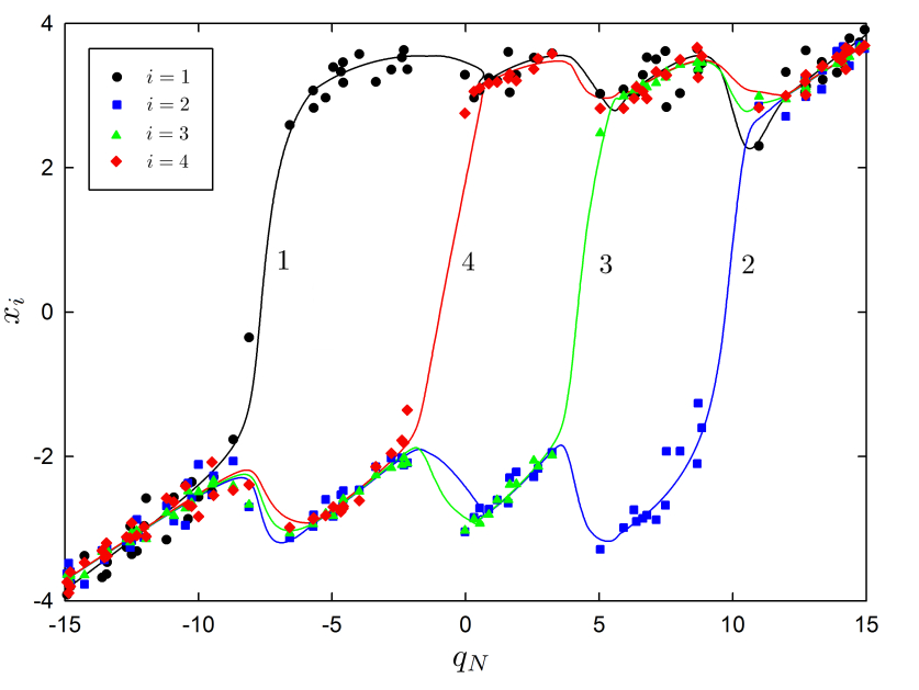
Figure 3: Evolution of the extensions of the different units in a pulling experiment as a function of the length of the system $q_{N}$. The pulling speed is $v_{p}=0.38$ and the length-control device has a stiffness $k_{p}=5$. The symbols correspond to a typical realization of the Langevin process (2) with $T=1$, whereas the lines correspond to the deterministic (zero noise) approximation.

To start with, we consider the relevance of the noise terms in (2). In figure 3, we plot the integration of the Langevin equations together with the deterministic approximation [32] for a concrete case: the free energy of the first unit corresponds to $\epsilon_{1}=0.8$ ($\xi=0.2$), the stiffness of the device controlling the length is $k_{p}=5$, the temperature is $T=1$ and the pulling speed is $v_{p}=0.38$. For these values of the parameters, taken from [17], the critical velocity in (37) is $v_{c}=1.4$, so we are considering a subcritical velocity, $v_{p}<v_{c}$. Thermal fluctuations are small, and thus the same unfolding pathway is observed in the deterministic and the majority of the stochastic trajectories.

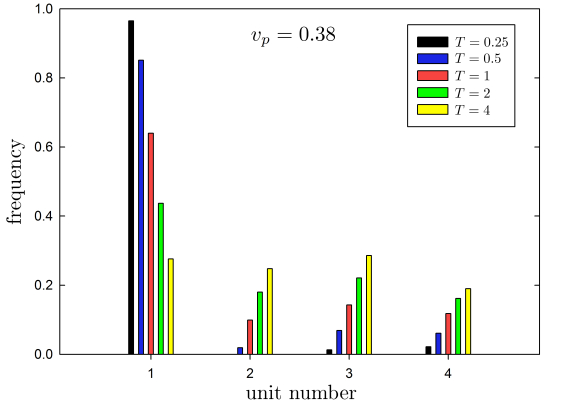
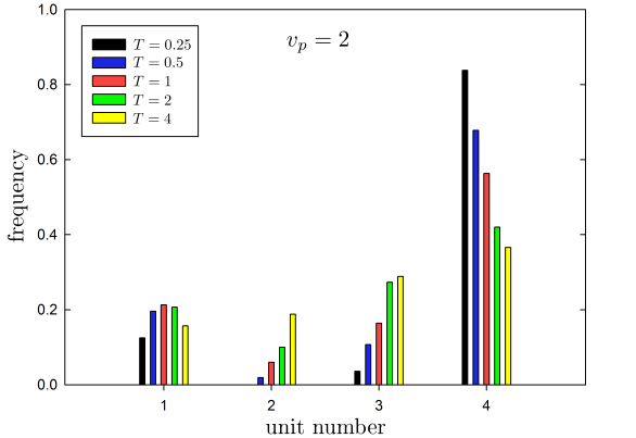
Figure 4: Frequency with which each of the units unfolds first when the Langevin equations with perfect length-control are integrated for different values of the temperature. (Left) Numerical frequencies obtained in $1000$ trajectories, for a subcritical pulling speed $v_{p}=0.38<v_{c}$. (Right) The same as in the left panel, but for a supercritical pulling speed $v_{p}=2>v_{c}$. As the temperature decreases, the frequency of the deterministic unfolding pathway approaches unity in both cases.

Let us consider in more detail the relevance of thermal noise: from a physical point of view, it may be inferred by looking at the height of the free energy barrier at the critical force in terms of the thermal energy $k_{B}T$. For the values of the parameters we are using, this barrier is around $20$ in reduced units. This explains why thermal noise is basically negligible in figure 3, in which $T=1$. If the temperature is decreased to $T=0.25$, the barrier is so high, around $80$ times the thermal energy, that essentially all the stochastic trajectories coincide with the deterministic one. On the other hand, if the temperature is increased to $T=4$, the barrier in only a few, around $5$, times the thermal energy, and we expect that the deterministic approximation ceases to be valid. In order to further clarify this point, we present figure 4. Both panels display bar graphs with the frequencies with which each unit unfolds first in the stochastic trajectories obtained over $1000$ trajectories of the Langevin equations (2) with perfect length control and different values of the temperature. In the left panel, a subcritical velocity $v_{p}=0.38<v_{c}$ is considered, so that the weakest (first) unit is expected to unfold first. In the right panel, the numerical data for a supercritical velocity $v_{p}=2>v_{c}$ are shown, for which the pulled (fourth) unit would unfold first. The effect of thermal noise is quite similar in both cases. For the low temperature $T=0.25$, the frequency of the deterministic pathway is close to unity and, for the temperature in figure 3, $T=1$, its frequency is still very large, clearly larger than any of the others. On the other hand, for the higher value of the temperature, $T=4$, thermal noise can no longer be neglected.

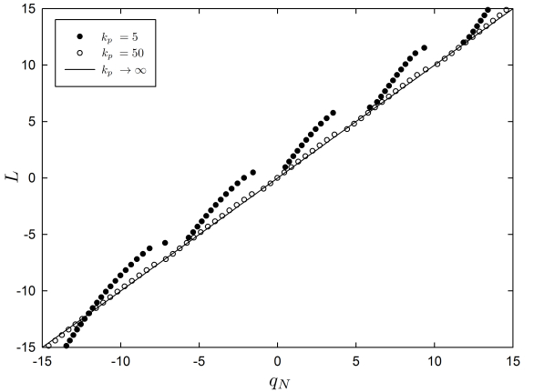
Figure 5: (Left) Evolution of the extensions of the different units in a pulling experiment as a function of the length of the system $q_{N}$. The symbols correspond to the integration of the deterministic equations, for $k_{p}=5$ (filled symbols) and $k_{p}=50$ (empty symbols), whereas the line correspond to the limit $k_{p}\to\infty$. The pulling speed is the same as in figure 3, that is, $v_{p}=0.38$. (Right) Comparison between the desired and actual lengths, $L$ and $q_{N}$, for the different values of the stiffness considered in the top panel. It is observed that the length control improves as $k_{p}$ increases.

In the following, we restrict the analysis to the physically relevant case in which the deterministic approximation gives a good description of the first unfolding event. In figure 5 (left panel), we look into the same pulling experiment as before, but now we compare the deterministic evolution of the extensions for two finite values of the stiffness to the $k_{p}\to\infty$ limit. Consistently with our expectations, the unfolding pathway is not affected by this simplification. Nevertheless, the control of the length of course improves as $k_{p}$ increases (see right panel). Although for the smaller values of $k_{p}$ the length is not perfectly controlled, the curves in the left panel, which correspond to different values of $k_{p}$, are almost perfectly superimposed when plotted as a function of the real length of the system $q_{N}$ (but not of the desired length $L$). This means that the real length $q_{N}$ is a good reaction coordinate, as already said in section 3.

We have integrated the deterministic approximation (6) (zero noise) of the Langevin equations for different values of the pulling speed, and extracted from them the numerical value of the critical velocity as a function of the asymmetry $\xi=1-\epsilon_{1}$. In order to obtain this numerical prediction, we initially set $v_{p}$ equal to the theoretical critical velocity given by (37). Then, we recursively shift it by a small amount $\delta v_{p}$, such that $\delta v_{p}/v_{c}=0.0001$, until the pathway changes. We compare the values so obtained to the theoretical expression (37), in figure 6. We find an excellent agreement for $\xi\lesssim 0.1$, for $\xi>0.1$ there appears some quantitative discrepancies. These discrepancies stem from two points: (i) the perturbative expansion used for obtaining (33) from (25) and (ii) the intrinsically approximate character of (25), since $\ell_{b}$ gives rigorously the limit of stability only for the static case $v_{p}=0$. Therefore, we have looked for the solution of (25) in the numerical integration of the deterministic equations. This is the dashed line in figure 6, which substantially improves the agreement between theory and numerics because we have eliminated the deviations arising from point (i) above. In fact, for the case we have studied in the previous figures, which corresponds to a not so small asymmetry $\xi=0.2$, the improved theory gives an almost perfect prediction for the critical velocity.

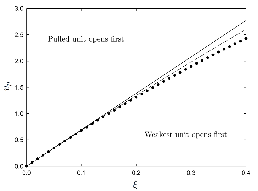
Figure 6: Phase diagram for the unfolding pathway in the pulling velocity-asymmetry plane. Two well-defined zones are separated by the curve giving the critical velocity $v_{c}$ as a function of the asymmetry $\xi$ in the free energy of the first unit. The numerical values for $v_{c}$ (circles) are compared to the theoretical expression (solid line), (37). The dashed line corresponds to the alternative approach discussed in the text, which improves the agreement between the numerical results and the theory for $\xi>0.1$. Error bars have been omitted because they are smaller than point size.

Now we consider a more realistic potential for the units, which has been introduced by Berkovich et al. for modelling the unfolding of single-unit I27 and ubiquitin proteins in AFM experiments [33, 34]. Moreover, it has also been used to investigate the stepwise unfolding of polyproteins in force-clamp conditions [35] and their force-extension curves in [27]. At zero force, it reads

$$U(x)=U_{0}\left[\left(1-e^{-2b(x-R_{c})/R_{c}}\right)^{2}-1\right]+\frac{k_{B}TL_{c}}{4P}\left(\frac{1}{1-\frac{x}{L_{c}}}-1-\frac{x}{L_{c}}+\frac{2x^{2}}{L_{c}^{2}}\right),$$ (38)

that is, it is the sum of a Morse and a worm-like-chain potentials, representing the enthalpic and the entropic contributions to the free energy, respectively [33, 34]. We take the values of the parameters from [27, 33], $P=0.4$nm (persistence length), $L_{c}=30$nm (contour length), $T=300$K, $U_{0}=100$pN nm($\sim\!\!24k_{B}T$), $R_{c}=4$nm, $b=2$. We measure force and extensions in the units $[F]=100$ pN, $L_{c}=30$ nm, respectively. Accordingly, dimensionless variables are introduced with the definitions $\mu=U_{0}/(L_{c}[F])$, $\beta=2bL_{c}/R_{c}$, $\rho=R_{c}/L_{c}$, $A=k_{B}TL_{c}/(4PU_{0})$. Thus, a dimensionless potential is obtained, which reads

$$U(x)=\mu\!\left\{\left[1-e^{-\beta(x-\rho)}\right]^{2}-1+A\!\left(\frac{1}{1-x}-1-x+2x^{2}\right)\right\},$$ (39)

Note that, in order not to clutter our formulae, we have not introduced a different notation for the dimensionless potential. The values of the parameters therein are $\mu=0.0333$, $\beta=30$, $\rho=0.133$ and $A=0.776$. In dimensionless variables, $F_{b}=0.527$ ($52.7$pN) and $\ell_{b}=0.157$ ($4.70$nm). The relevant time scale is set by the friction coefficient $\gamma$, $[t]=\gamma L_{c}/[F]$. In turn, $\gamma$ is given by the Einstein relation $D=k_{B}T/\gamma$, where $D$ is the diffusion coefficient for tethered proteins in solution. We consider a typical value of $D$, also taken from [33], $D=1500$ nm²/s, so that $\gamma=0.0028$pN nm^-1 s.

We consider a system of $4$ units, again with all the units but the first being identical. Then, $U_{i}(x)=U(x)$, $i\neq 1$, and the first unit is the weakest because $U_{1}(x)=(1-\xi)U(x)$. The situation is then similar to the one we have already analyzed with the quartic potential (34), but there is a difference that should be noted: here, $U(x)$ is the free energy at zero force, whereas for the quartic potential $U(x)$ was the free energy at a force $F_{0}$ for which the folded and unfolded minima were equally deep. Then, the force here must not be interpreted as the extra force from $F_{0}$, but as the whole force that is applied to the polyprotein. On the basis of our theory, we expect the simplest situation with only one critical velocity $v_{c}$, below (above) which the weakest unit (the pulled unit) unfolds first. This is also indeed the case in the numerical simulations, and we compare the theoretical and numerical critical velocities in figure 7. A very good agreement is found again, up to values of the asymmetry $\xi$ of the order $0.1-0.2$.

The above discussion shows that the validity of the theory presented here is not restricted to simple potentials like the quartic one; on the contrary, it can be confidently applied to experiments in which the units are described by realistic potentials. Moreover, for the typical parameters we are using, the theoretical critical velocity $v_{c}$ for the Berkovich potential equals $1270$nm/s for an asymmetry $\xi=0.1$, which can be regarded as quite a conservative estimate of the largest asymmetries for which our theory gives an almost perfect description of the unfolding pathway. Interestingly, this pulling speed corresponds to the upper range of velocities usually employed in AFM experiments, for instance see Table I of [4]. Therefore, testing our theory in real AFM experiments with modular proteins should be achievable.

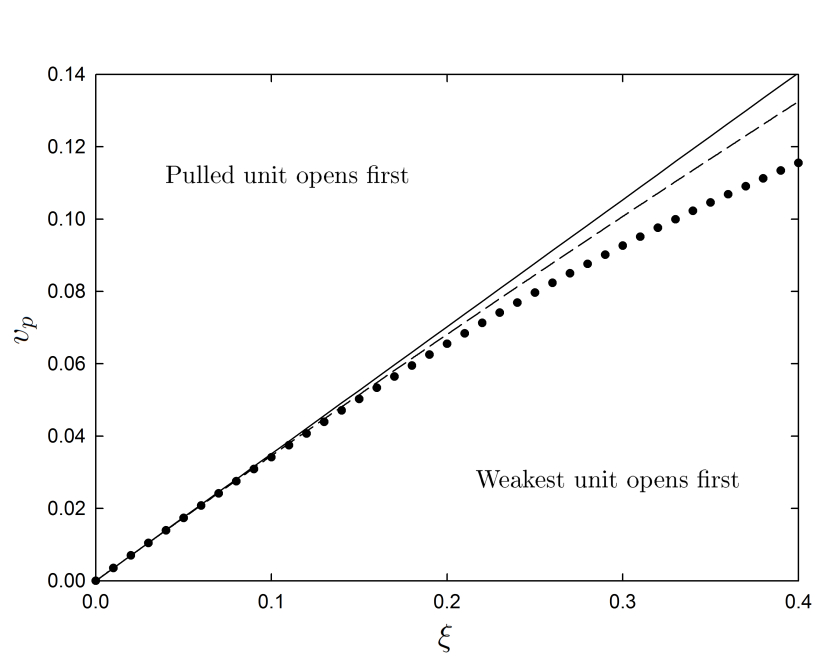
Figure 7: Phase diagram for the unfolding pathway in the pulling velocity-asymmetry plane for the Berkovich potential, (39). Again, as in figure 6, there appear two well-defined pulling regimes, separated by the curve giving the critical velocity $v_{c}$ as a function of the asymmetry $\xi$. The numerical values for $v_{c}$ (circles) compare very well with the theoretical expression (solid line), (33). Again, the dashed line corresponds to the alternative approach discussed in the text for the quartic potential, which once more significantly improves the agreement theory-simulation for the larger values of $\xi$.

Finally, we consider a more complex situation, in which more than one unit is different from the rest and there may exist more than one critical velocity. To be concrete, we have considered a system with $4$ units in which $U_{2}(x)=U_{3}(x)=U(x)$, $U_{1}(x)=(1-\xi)U(x)$ as before but $U_{4}(x)=(1+3\xi/2)U(x)$, with $U(x)$ being the quartic potential in (34). In this situation, we have two different critical velocities: for very low pulling speeds, the weakest unit is the first to unfold, but there appears a velocity window inside which neither the weakest nor the pulled unit is the first to unfold. This stems from the fact that the first and the third unit reach simultaneously the limit of stability for a velocity $v^{1}(3)=4\xi\gamma^{-1}F_{b}/3$ that is smaller than the velocity $v^{1}(4)=5\xi\gamma^{-1}F_{b}/3$ for which the first and the last would do so. The physical reason behind this is the threshold force of the pulled unit being larger enough than that of the third one. We recall that $v^{i}(j)$ is the velocity for which the $i$-th and the $j$-th unit reach simultaneously their limits of stability. Afterwards, the third unit and the fourth attain the limit of stability in unison for a velocity $v^{3}(4)=2\xi\gamma^{-1}F_{b}$, and the following picture emerges from our theory. Using the notation introduced in section 3.3, we define two critical velocities,

$$\frac{\gamma v_{c}^{(1)}}{\xi}=\frac{4F_{b}}{3},\qquad\frac{\gamma v_{c}^{(2)}}{\xi}=2F_{b},$$ (40)

such that for $v_{p}<v_{c}^{(1)}$, it is the weakest unit that unfolds first, for $v_{c}^{(1)}<v_{p}<v_{c}^{(2)}$, it is the third unit that unfolds first, and, finally, for $v_{p}>v_{c}^{(2)}$, the first unit to unfold is the pulled one.

We check the more complex scenario described in the previous paragraph in figure 8. Therein, we observe that (i) our theory correctly predicts the existence of the three pulling regimes described above but (ii) even for very small asymmetries, there appear some noticeable discrepancy between theory and simulation. Since the validity of the perturbative expansion for obtaining the critical velocities from the condition (25) is strongly supported by the accurateness of the theoretical prediction for the simplest case, see figures 6 and 7, this discrepancy should stem from the intrinsically approximate character of the condition $U^{\prime\prime}_{i}=0$ for determining the stability threshold when $v_{p}\neq 0$. Therefore, an improvement of the present theory should involve the derivation of a more accurate condition for obtaining the stability threshold in the case of finite pulling velocity. This point, which probably makes a multiple scale analysis necessary for lengths close to the condition $U^{\prime\prime}=0$, certainly deserves further investigation.

Figure 8: Phase diagram for the unfolding pathway in the pulling velocity-asymmetry plane for the more complex case discussed in the text. Now, we have three well-defined pulling regimes, separated by two curves giving the critical velocities $v_{c}^{(1)}$ and $v_{c}^{(2)}$ as a function of the asymmetry $\xi$. In this case, our theoretical approach is able to reproduce the existence of the three different pulling regimes, but the discrepancies between the theoretical and the numerical values for the critical velocities are larger than in the simpler cases considered in the previous figures.

5 Conclusions

We have investigated the general properties of the unfolding pathway in pulled proteins by means of a simple model portraying the chain as a sequence of nonlinear modules. The deterministic approximation of the Langevin equations controlling the time evolution of the units extensions is used therein. This is a sensible approach in our model system: note that the free energies characterising the different units are considered to be very similar, and therefore their Kramers rates for thermal activated unfolding would also be very close. Then, were thermal effects important, our unfolding trajectories would be essentially stochastic and we would not observe a specific unfolding pathway.

Nevertheless, in some recent optical tweezers experiments in which thermal fluctuations are relevant, definite pathways have also been observed. Although trajectories are indeed stochastic, the pathway is well-characterised [45, 46]. Therefore, the analysis of these experiments needs a more sophisticated theory, which takes into account thermal noise effects. Moreover, it seems that there are other elements that should be incorporated, such as (i) the possible coupling between the different units and (ii) their dissimilar free energies. For example, the former may explain the existence of dead ends observed in [46], that is, intermediate states that do not allow the system to completely relax, whereas the latter may lead to Kramers rates leading to the separation of the timescales for the different unfolding events.

The equilibrium extensions of the units are governed by different free energies, which we have called asymmetry or disorder in the free energies. Our theory, based on stability considerations, is able to explain the experimental observations: (i) for low pulling speeds, it is the weakest unit that unfolds first, (ii) for large enough pulling speed, it is the pulled unit that opens first. This has been done by introducing a perturbative expansion both in the asymmetry of the free energies and in the pulling speed. Moreover, our approach makes it possible to identify a critical rate that separates two well-defined regimes. To the lowest order, this critical velocity has a linear dependence on the asymmetry of the potential. In spite of the crude approximations, our theory compares quite well with the numerical data even beyond the applicability regime. Moreover, our results provide a guide to interpret some inversions observed in the sequence of unfolding of the stable regions of the maltose-binding protein during its mechanical denaturation [17, 23].

It must be stressed that to the lowest order in our theory, the system is sweeping the stationary branches of the force-extension curve. In this sense, the pulling process is very slow or adiabatic. Despite this adiabatic nature of the pulling process, it is not always the weakest unit to unfold first. As long as the pulling speed $v_{p}\neq 0$, the closer to the pulled terminal one unit is, the larger the force acting on it. This gradient in the distribution of the force across the protein, which increases with the pulling speed, makes it possible that the last unit reaches first its limit of stability.

We have limited ourselves to the investigation of the first unfolding event. However, our argument can be easily generalized to the next unfolding event: the difference is that the zero-th order approximation is no longer given by all the units sweeping the all-units-folded branch but by the sweeping of the branch with one module unfolded and the remainder folded. Then, a similar perturbative expansion around this zero-th order solution in powers of the asymmetry and the pulling speed would give the next unit that opens.

If the biomolecule comprises several perfectly identical units, the asymmetry correction vanishes, because $\delta U_{i}=0$ (and thus $\delta f_{i}=0$) for all the units. In that case, our theory predicts that it is always the pulled unit that unfolds first. However, even in engineered modular proteins, slight differences from module to module may be present. In fact, this has lead to the analysis of the impact of quenched disorder in the force-extension curves of biomolecules [27]. In the present context, we may also introduce stochastic free energy deviations, following a certain probability distribution. Next, our theoretical approach can be applied to this system with quenched disorder in the free energies. Interestingly, evidence of dynamical disorder, that is, a fluctuating environment, has been recently brought to bear in stretching experiments [47]. The analysis of this situation needs a more complex theory, in which the free energy landscape fluctuates in time, and is outside of the scope of the present paper.

There are methods that extract the free energy landscape from experimental data of pulling experiments, even when there are intermediates [36, 37, 38, 39, 40]. The resulting free energy is usually calculated as a function of the end-to-end distance of the molecule. Nevertheless, in order to apply our theory, we do not need this global energy landscape as a function of the end-to-distance of the molecule but each unit’s contribution thereto as a function of its own extension. In this regard, it is relevant to note that a similar velocity dependent unfolding pathway should also be found in modular proteins, although it has not been experimentally investigated to the best of our knowledge. In fact, we have analyzed a simple polyprotein model with a realistic potential, and observed a completely analogous behaviour. When all the modules are not identical, the weakest one will always open first for small enough pulling velocities. On the other hand, if the pulled unit is not the weakest, this will no longer be the case as the pulling speed is increased. Since the free energy of each module is experimentally accessible and the critical velocity lies on the experimental range, a reliable test of our theory could be done in modular proteins. Another possibility that deserves attention is to test our theory in ankyrin repeat proteins. In [48], the unfolding of a consensus ankyrin repeat protein, NI6C, has been investigated. This protein is composed of eight repeats: the two capping repeats are different from the six identical central ones, that at the C-terminus (N-terminus) is weaker (stronger) than the rest. Pulling from the C-terminus (weakest unit), Lee et al. observe that the unfolding always starts from this end. This is what is expected from our theory, since when the pulled and the weakest units coincide, there is no competition between the asymmetry and kinetic terms. Therefore, it seems relevant to carry out the same experiment but pulling from the N-terminus (strongest unit), in which a much richer phenomenology is to be expected.

Very recently, sequential unfolding has been reported in a simple model [35], which makes it possible to understand the stepwise unfolding observed in force-clamp experiments with modular proteins [41, 42, 43]. This sequential unfolding appeared as a consequence of a depinning transition near the stability threshold introduced by the coupling between nearest neighbour units. Interestingly, the unfolding of the ankyrin repeat protein in [48] does not only start from a well-defined end but it is also sequential, which may hint at the significance of this kind of short-ranged couplings in the experiment. Then, it seems also relevant to analyze whether a similar sequential unfolding is present in the model developed here, when a similar short ranged interaction between neighbouring units is considered.

Appendix A Stability threshold

To first order in $\xi$, the extension $x_{i,b}$ such that $U^{\prime\prime}_{i}(x_{i,b})=0$ verifies

$$U^{\prime\prime\prime}(\ell_{b})(x_{i,b}-\ell_{b})+\xi\delta\!f^{\prime}_{i}(\ell_{b})=0,$$ (41)

that is,

$$x_{i,b}=\ell_{b}-\xi\frac{\delta\!f^{\prime}_{i}(\ell_{b})}{U^{\prime\prime\prime}(\ell_{b})}.$$ (42)

The corresponding force at the stability threshold is obtained from (10). To the lowest order in the deviations,

$$F_{i,b}\equiv U^{\prime}_{i}(x_{i,b})\sim U^{\prime}_{i}(\ell_{b})=F_{b}+\xi\,\delta\!f_{i}(\ell_{b}),$$ (43)

because the next term, $U^{\prime\prime\prime}(\ell_{b})(x_{i,b}-\ell_{b})^{2}/2$, is of the order of $\xi^{2}$. Therefore, the $i$-th module reaches its limit of stability at the time for which $x_{i}=x_{i}^{(0)}+\xi\delta x_{i}=x_{i,b}$, that is, when the length per unit $\ell$ has the value $\ell_{i}$ verifying

$$\ell_{i}+\xi\frac{\overline{\delta\!f}(\ell_{i})-\delta\!f_{i}(\ell_{i})}{U^{\prime\prime}(\ell_{i})}=\ell_{b}-\xi\frac{\delta\!f^{\prime}_{i}(\ell_{b})}{U^{\prime\prime\prime}(\ell_{b})},$$ (44)

or, equivalently,

$$\ell_{i}-\ell_{b}=\xi\frac{\delta\!f_{i}(\ell_{i})-\overline{\delta\!f}(\ell_{i})}{U^{\prime\prime}(\ell_{i})}-\xi\frac{\delta\!f^{\prime}_{i}(\ell_{b})}{U^{\prime\prime\prime}(\ell_{b})}.$$ (45)

We know that $\ell\to\ell_{b}$ when $\xi\to 0$. But $U^{\prime\prime}(\ell_{b})=0$ and thus we cannot substitute $\ell_{b}$ on the rhs of (45). On the other hand, this means that the dominant balance for $\xi\to 0$ involves the lhs and the first term on the rhs of (45). Therefore, making use of $U^{\prime\prime}(\ell)\sim U^{\prime\prime\prime}(\ell_{b})(\ell-\ell_{b})$, we get

$$(\ell_{i}-\ell_{b})^{2}\sim\xi\frac{\delta\!f_{i}(\ell_{b})-\overline{\delta\!f}(\ell_{b})}{U^{\prime\prime\prime}(\ell_{b})}.$$ (46)

Since $U^{\prime\prime\prime}(\ell_{b})<0$ (see figure 2), this means that only the units with $\delta\!f_{i}(\ell_{b})$ smaller than the average (that is, weaker than average) reach the limit of stability in the limit as $v_{p}\to 0$. In fact, it is the weakest unit, that is, the unit with smallest $\delta\!f_{i}(\ell_{b})$, that unfolds first.

It is interesting to note that, in order to obtain (46), we have completely neglected the last term on the rhs of (45). Since, in turn, this term stems from the last term on the rhs of (42), to the lowest order we are solving the equation $x_{i}=\ell_{b}$. In other words, to the lowest order the stability threshold can be considered to be given by the non-disordered, zero-asymmetry case, free energy $U(x)$. For the sake of concreteness and simplicity, we have stuck to the asymmetry contribution $\delta x_{i}$ in this appendix, but the same condition $x_{i}=\ell_{b}$ would still be valid, had we taken into account the kinetic contribution $\Delta x_{i}$ derived in section 3.2. The reason is that there is also a factor $U^{\prime\prime}(\ell)$ in the denominator of $\Delta x_{i}$, see (23a), and thus both the terms coming from $\delta x_{i}$ and $\Delta x_{i}$ are dominant against the last term on the rhs of (42).

Appendix B Discrete inhomogeneous diffusion equation

In this appendix, we briefly discuss a general procedure which is useful to solve linear difference equations similar to those in (19) and (22). The methods for solving difference equations often resemble those used for solving analogous differential equations; the latter may be thought of as the continuous limit of the former. Both (19) and (22) belong to the following general class of second-order linear difference equations for $y_{i}$,

$$y {}_{1}=g(y_{2},\ldots,y_{N-1}),$$ (47a)

$$y {}_{i+1}+y_{i-1}-2y_{i}=K,\quad 1<i<N,$$ (47b)

$$y {}_{N}=h(y_{2},\ldots,y_{N-1}),$$ (47c)

in which $g$, $h$ are arbitrary functions and $K$ is a given constant. (47b) is a second-order linear difference equation, and (47a) and (47c) are its boundary conditions. It may be thought of as a discrete inhomogeneous diffusion equation: $y_{i+1}-y_{i}$ is the first discrete derivative, so that $y_{i+1}+y_{i-1}-2y_{i}$ is the second discrete derivative [31]. In complete analogy with the corresponding differential equation $y^{\prime\prime}=K$, the general solution of (47b) is

$$y_{i}=c_{0}+c_{1}i+\frac{K}{2}i^{2},$$ (48)

in which $c_{0}$ and $c_{1}$ are two arbitrary constants. The solution of (47) is, as usual, univocally determined by the boundary conditions, from which specific values for $c_{0}$ and $c_{1}$ are obtained.

Let us show that both (19) and (22) can be cast in the above form. Firstly, in (19b), it is easily seen that if we define $y_{i}=\delta x_{i}+\delta f_{i}/U^{\prime\prime}(\ell)$, (47b) is obtained with $K=0$. Secondly, in (22b), it is straightforward to identify $y_{i}=\Delta x_{i}$ and $K=\gamma[NU^{\prime\prime}(\ell)]^{-1}$. A simple calculation gives the constants $c_{0}$ and $c_{1}$ in (48) for each case, and thus the expressions for $\delta x_{i}$ and $\Delta x_{i}$ in the main text.

Appendix C Order of the critical velocities

Here, we prove that $v_{c}^{(k+1)}>v_{c}^{(k)}$. It is easy to show that this inequality follows if we have that

$$\delta\!f_{\alpha_{k+2}}(\ell_{b})>\frac{\delta\!f_{\alpha_{k+1}}(\ell_{b})(\nu_{k+2}-\nu_{k})-\delta\!f_{\alpha_{k}}(\ell_{b})(\nu_{k+2}-\nu_{k+1})}{\nu_{k+1}-\nu_{k}},$$ (49)

in which $\nu_{k}=\alpha_{k}(\alpha_{k}-1)$. Due to (31), $\alpha_{k+1}$ minimize $v^{\alpha_{k}}(j)$. Therefore, in particular, $v^{\alpha_{k}}(\alpha_{k+1})<v^{\alpha_{k}}(\alpha_{k+2})$, which is readily shown to be equivalent to (49).

References

- [1] Ritort F, 2006 J. Phys: Condens. Matter 18, R531
- [2] Kumar D and Li M S, 2010 Phys. Rep. 486 1
- [3] Marszalek P E and Dufrˆene Y F, 2012 Chem. Soc. Rev. 41, 3523
- [4] Hoffmann T and Dougan L, 2012 Chem. Soc. Rev. 41, 4781
- [5] Smith S B, Cui Y and Bustamante C, 1996 Science 271, 795
- [6] Lu H and Schulten K, 1999 Proteins Struct. Funct. Genet. 35, 453
- [7] Manosas M and Ritort F, 2005 Biophys. J. 88, 3224-3242
- [8] Cao Y, Kuske R and Li H, 2008 Biophys. J. 95, 782
- [9] Carrion-Vazquez M, Oberhauser A F, Fowler S B, Marszalek P E, Broedel S E, Clarke J and Fernandez J M, 1999 Proc. Natl. Acad. Sci. USA 96, 3694
- [10] Fisher T E, Marszalek P E and Fernandez J M, 2000 Nat. Struct. Biol. 7, 719
- [11] Liphardt J, Onoa B, Smith S B, Tinoco I and Bustamante C, 2001 Science 292, 733
- [12] Bustamante C, Bryant Z and Smith S B, 2003 Nature 421, 423
- [13] Klimov D K and Thirumalai D, 2000 Proc. Natl. Acad. Sci. USA 97, 7254
- [14] Hyeon C, Dima R I, and Thirumalai D, 2006 Structure 14, 1633
- [15] Liphardt J, Dumont S, Smith S B, Tinoco I and Bustamante C, 2002 Science 296, 1832
- [16] Li M S and Kouza S, 2009 J. Chem. Phys. 130, 145102
- [17] Guardiani C, Di Marino D, Tramontano A, Chinappi M and Cecconi F, 2014 J. Chem. Theory Comput. 10, 3589
- [18] Kouza M, Hu C K, Li M S and Kolinski A, 2013 J. Chem. Phys. 139, 065103
- [19] Bertz M and Rief M, 2008 J. Mol. Biol. 378, 447
- [20] Bacci M, Chinappi M, Casciola C M and Cecconi F, 2012 J. Phys. Chem. B 116, 4255
- [21] Bacci M, Chinappi M, Casciola C M and Cecconi F, 2013 Phys. Rev. E 88, 022712
- [22] Merstorf C, Cressiot B, Pastoriza-Gallego M, Oukhaled A, Betton J M, Auvray L and Pelta J, 2012 ACS Chem. Biol. 7, 652
- [23] Aggarwal V, Kulothungan S R, Balamurali M M, Saranya S R, Varadarajan R and Ainavarapu S R K, 2011 J. Biol. Chem. 286 28056
- [24] Kotamarthi H C, Narayan S and Ainavarapu S R K, 2014 J. Phys. Chem. B 118, 11449
- [25] Prados A, Carpio A and Bonilla L L, 2013 Phys. Rev. E 88, 012704
- [26] Bonilla L L, Carpio A and Prados A, 2015 EPL 108 28002
- [27] Bonilla L L, Carpio A and Prados A, 2015 Phys. Rev. E 91, 052712
- [28] Hummer G and Szabo A, 2003 Biophys. J. 85, 5
- [29] Dudko O K, Hummer S and Szabo A, 2006 Phys. Rev. Lett. 96, 108101
- [30] Arad-Haase G, Chuartzman S G, Dagan S, Nevo R, Kouza M, Mai B K, Nguyen H T, Li M S and Reich Z, 2010 Biophys. J. 99, 238
- [31] Bender C M and Orszag S A 1999 Advanced Mathematical Methods for Scientists and Engineers, (Springer, New York), chapter 2
- [32] van Kampen N G 1997 Stochastic Processes in Physics and Chemistry (North-Holland, Amsterdam)
- [33] Berkovich R, Garcia-Manyes S, Urbakh M, Klafter J and Fernandez J M, 2010 Biophys. J. 98, 2692
- [34] Berkovich R, Hermans R I, Popa I, Stirnemann G, Garcia-Manyes S, Bernes B J and Fernandez J M, 2012 Proc. Nat. Acad. Sci. 109, 14416
- [35] Bonilla L L, Carpio A and Prados A, 2014 EPL 108, 28002
- [36] Bustamante C, Chemla Y R, Forde N R and Izhaky D, 2004 Annu. Rev. Biochem. 73, 705
- [37] Li M S, Gabovich A M and Voitenko A I, 2008 J. Chem. Phys. 129, 105102
- [38] Alemany A, Mossa A, Junier I and Ritort F, 2012 Nature Physics 8, 688
- [39] Hinczewskia M, Gebhardtb J C M, Rief M, and Thirumalai D, 2013 Proc. Nat. Acad. Sci. 110, 4500
- [40] Manuela A P, Lamberta J, and Woodside M T, 2015 Proc. Nat. Acad. Sci. 112, 7183
- [41] Fernandez J M and Li H, 2004 Science 303, 1674
- [42] Walther K A, Gräter F, Dougan L, Badilla C L, Berne B J and Fernandez J M, 2007 Proc. Natl. Acad. Sci. 104, 7916
- [43] Lannon H, Haghpanah J S, Montclare J K, Vanden-Eijnden E and Brujic J, 2013 Phys. Rev. Lett. 110, 128301
- [44] Rico F, Gonzalez L, Casuso I, Puig-Vidal M and Scheuring S, 2013 Science 342, 8
- [45] Neupane K, Yu H, Foster D A N, Wang F and Woodside M T, 2011 Nucleic Acids Research 39, 7677.
- [46] Stigler J, Ziegler F, Gieseke A, Christof J, Gebhardt M and Rief M, 2011 Science 334, 512
- [47] Hyeon C, Hinczewski M and Thirumalai D, 2014 Phys. Rev. Lett.112, 138101
- [48] Lee W, Zeng X, Zhou H X, Bennett V, Yang W and Marszalek P E, 2010 J. Biol. Chem. 285, 38167