Interacting quantum walkers: Two-body bosonic and fermionic bound states

Abstract

We investigate the dynamics of bound states of two interacting particles, either bosons or fermions, performing a continuous-time quantum walk on a one-dimensional lattice. We consider the situation where the distance between both particles has a hard bound, and the richer situation where the particles are bound by a smooth confining potential. The main emphasis is on the velocity characterizing the ballistic spreading of these bound states, and on the structure of the asymptotic distribution profile of their center-of-mass coordinate. The latter profile generically exhibits many internal fronts.

,,

1 Introduction

Quantum walks have witnessed an upsurge of interest in parallel with the developments of quantum algorithms and quantum information (see [1, 2, 3] for reviews). Two different types of quantum-mechanical analogues of classical random walks have been investigated. Discrete-time quantum walkers [4, 5, 6, 7] possess, besides their spatial position, a finite-dimensional internal degree of freedom, referred to as a quantum coin. Both spatial and internal degrees of freedom jointly undergo a unitary dynamics. Continuous-time quantum walkers [8, 9, 10] have no internal degree of freedom. Their dynamics is governed by some hopping operator on the underlying structure. Despite these differences, continuous-time quantum walks can be viewed as a limit of discrete-time quantum walks [11]. Both types of quantum walks exhibit many similar properties. Their main characteristic feature is a fast ballistic spreading. The typical distance traveled by a quantum walker grows linearly in time, as opposed to the diffusive spreading of a classical random walker.

If two or more quantum walkers are simultaneously present, the combined effects of interactions, quantum statistics and entanglement give rise to novel features which have no classical counterpart. The Anderson localization of two interacting quantum particles in a random potential has attracted much attention [12, 13, 14]. More recently, dynamical features of the quantum walks performed by two or more entangled or interacting particles have been the subject of numerous theoretical studies (see e.g. [15, 16, 17, 18, 19, 20, 21, 22, 23, 24, 25]). Several experimental groups have also studied the quantum walk of entangled pairs of magnons [26] and of photons in various integrated photonics devices [27, 28, 29, 30].

Here we investigate the continuous-time quantum walk of bound states of two identical bosonic or fermionic particles. The main emphasis is on the distribution profile in the center-of-mass coordinate of the bound states, including the dependence of the ballistic spreading velocity on model parameters, and the generic presence of many internal ballistic fronts. The setup of this paper is as follows. In section 2 we revisit in a pedagogical way the continuous-time quantum walk of a single particle. We analyze the distribution of the position of the particle, emphasizing its dependence on the initial quantum state. We also show that allowing the particle to hop to second neighbors may yield a novel effect, namely the appearance of internal ballistic fronts in the position distribution, besides the usual extremal fronts. We then address similar questions in the more challenging situation of the quantum walk performed by bound states of two identical particles. The same formalism allows one to deal with bosonic and fermionic bound states, as they are respectively described by even and odd functions of the relative coordinate between both particles. We consider bound states generated either by imposing a hard bound on the distance between both particles (section 3) or by a smooth confining potential (section 4). In both situations the emphasis is on the distribution of the center-of-mass coordinate and on the presence of internal ballistic fronts. Section 5 contains a discussion of our findings.

2 Quantum walk of a single particle

This section serves as a self-contained pedagogical introduction to the main concepts emphasized in the rest of the paper. We consider the continuous-time quantum walk performed by a single particle on a one-dimensional lattice. Most of the features underlined in this section have been studied, or at least mentioned, in several earlier works in the context of discrete-time quantum walks [20, 31, 32, 33, 34, 35, 36, 37]. One of the purposes of this section is to demonstrate that the analysis of the continuous-time quantum walk problem is much simpler, and can therefore be worked out in a more systematic fashion.

More specifically, we first revisit the simple quantum walk where the particle hops to nearest neighbors only, focusing our attention onto the asymptotic distribution of the walker, including its dependence on the initial state. We then turn to a generalized quantum walk, where the particle hops to further neighbors as well. We show that allowing hopping to second neighbors gives rise to internal fronts in the distribution profile. Hopping to second neighbors is known to have drastic physical consequences in many other situations. One celebrated example is graphene (see [38, 39]), where hopping to second neighbors breaks the chiral symmetry between both sublattices.

2.1 Simple quantum walk

The framework of the simple quantum walk is the usual one of the tight-binding approximation, where the particle hops to nearest neighbors only. Throughout this paper, we use dimensionless units. The wavefunction $\psi_{n}(t)=\langle n|\psi(t)\rangle$ of the particle at site $n$ at time $t$ obeys

$${\rm i}\,{\frac{{\rm d}\psi_{n}(t)}{{\rm d}t}}=\psi_{n+1}(t)+\psi_{n-1}(t).$$ (2.1)

The dispersion law between wavevector (momentum) $q$ and frequency (energy) $\omega$ and the corresponding group velocity $v$ therefore read

$$\omega(q)=2\cos q,\qquad v(q)=\omega^{\prime}(q)=-2\sin q,$$ (2.2)

where the prime denotes a derivative.

Initial state localized at the origin

Suppose that at time $t=0$ the particle is localized on a single site, taken as the origin of the lattice: $\psi_{n}(0)=\delta_{n,0}$. In Fourier space, $\widehat{\psi}(q,0)=1$, hence $\widehat{\psi}(q,t)=\rme^{-{\rm i}\omega(q)t}$, and so

$$\psi_{n}(t)=\int_{0}^{2\pi}\frac{{\rm d}q}{2\pi}\,\rme^{{\rm i}(nq-2t\cos q)}={\rm i}^{-n}\,J_{n}(2t),$$ (2.3)

where the $J_{n}$ are the Bessel functions.

Figure 1 shows the probabilities $|\psi_{n}(t)|^{2}=(J_{n}(2t))^{2}$ against position $n$ at time $t=50$. These probabilities exhibit various regimes of behavior at large $n$ and $t$. They take appreciable values in the allowed region which spreads ballistically with the maximal velocity

$$V=\mathrel{\mathop{{\rm max}}\limits_{q}}|\omega^{\prime}(q)|=2.$$ (2.4)

Furthermore, they exhibit sharp fronts near $n=\pm 2t$, and they decay exponentially in the forbidden region beyond these fronts. These asymptotic results are classics of the theory of Bessel functions [40, 41], whose physical meaning has been underlined in [9]. These results can be readily obtained the saddle-point method, which will be used later in other situations.

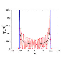
Figure 1: Probability profile $|\psi_{n}(t)|^{2}$ at time $t=50$ for the simple quantum walk with a particle initially located at the origin. Vertical blue lines: theoretical positions of the ballistic fronts. Black curve: asymptotic distribution (2.7) set to scale.

• Allowed region ($|n|<2t$). In this region, the oscillatory behavior of the wavefunction at long times can be derived as follows. Setting

  $$n=-2t\sin{q_{\star}}\qquad\left(|{q_{\star}}|<\pi/2\right),$$ (2.5)

  the integral in (2.3) is dominated by two equivalent saddle points at $q={q_{\star}}$ and $q=\pi-{q_{\star}}$ (modulo $2\pi$). We thus recover the well-known asymptotic form of Bessel functions:

  $$J_{n}(2t)={\rm i}^{n}\psi_{n}(t)\approx\frac{\cos(2t\cos{q_{\star}}-n(\pi/2+{q_{\star}})+\pi/4)}{\sqrt{\pi t\cos{q_{\star}}}}.$$ (2.6)

  By averaging out the oscillations in the probabilities $|\psi_{n}(t)|^{2}$, one arrives [9] at a smooth distribution $f(v)$ for the ratio $v=n/t$ in the long-time limit, i.e.,

  $$f(v)=\frac{1}{\pi\sqrt{4-v^{2}}}\qquad(|v|<2).$$ (2.7)

  The above result can be alternatively obtained by folding the uniform distribution on the Brillouin zone $[-\pi,\pi]$ by the dispersion curve of the group velocity: $v=-2\sin q$.

• Transition region ($|n|\approx 2t$). The distribution (2.7) becomes singular as the endpoints of the allowed region are approached ($n\to\pm 2t$). The vicinity of these endpoints corresponds to the transition region in the theory of Bessel functions. Setting $|n|=2t+zt^{1/3}$, we have

  $$J_{n}(2t)={\rm i}^{n}\psi_{n}(t)\approx t^{-1/3}{\rm Ai}(z),$$ (2.8)

  where ${\rm Ai}(z)$ is the Airy function. The probabilities $|\psi_{n}(t)|^{2}$ therefore exhibit sharp ballistic fronts [9], whose height and width respectively scale as $t^{-2/3}$ and $t^{1/3}$.

• Forbidden region ($|n|>2t$). In this region, the exponential fall-off of the wavefunction at long times can be derived by evaluating again the integral in (2.3) by the saddle-point method. Setting $|n|=2t\cosh\theta$ with $\theta>0$, we obtain

  $$J_{n}(2t)={\rm i}^{n}\psi_{n}(t)\approx\frac{\rme^{-2t(\theta\cosh\theta-\sinh\theta)}}{\sqrt{4\pi t\sinh\theta}}.$$ (2.9)

Arbitrary initial state

For an arbitrary initial state $\psi_{n}(0)$, we have

$$\psi_{n}(t) = \int_{0}^{2\pi}\frac{{\rm d}q}{2\pi}\,\rme^{{\rm i}(nq-2t\cos q)}\widehat{\psi}(q,0)$$ (2.10)

$$= \sum_{m}{\rm i}^{m-n}\,\psi_{m}(0)J_{n-m}(2t).$$

Whenever the initial state is reasonably localized, in the sense that $\psi_{n}(0)$ decays fast enough with distance $|n|$, the time-dependent wavefunction exhibits qualitatively the regimes of behavior described above in the allowed region, ballistic fronts, and forbidden region.

Let us analyze more carefully the allowed region ($|n|<2t$). With the definition (2.5), the integral in (2.10) is now dominated by two inequivalent saddle points at $q={q_{\star}}$ and $q=\pi-{q_{\star}}$ (modulo $2\pi$). We thus arrive at

$$\psi_{n}(t)\approx\frac{1}{\sqrt{4\pi\cos{q_{\star}}}}\Bigl{(} \widehat{\psi}({q_{\star}},0)\,\rme^{{\rm i}(n{q_{\star}}-2t\cos{q_{\star}}+\pi/4)}$$ (2.11)

$$+\widehat{\psi}(\pi-{q_{\star}},0)\,\rme^{{\rm i}(n(\pi-{q_{\star}})+2t\cos{q_{\star}}-\pi/4)}\Bigr{)}.$$

Averaging out the oscillations in the above expression yields the following formula for the locally coarse-grained probabilities:

$$|\psi_{n}(t)|^{2}\approx\frac{|\widehat{\psi}({q_{\star}},0)|^{2}+|\widehat{\psi}(\pi-{q_{\star}},0)|^{2}}{4\pi t\cos{q_{\star}}}.$$ (2.12)

The limit distribution $f(v)$ of the ratio $v=n/t$ is obtained by folding the distribution on the Brillouin zone with density $|\widehat{\psi}(q)|^{2}/(2\pi)$ by the dispersion curve $v=-2\sin q$. This line of thought has been used in [35, 36], and more thoroughly in [37], for discrete-time walks.

For definiteness, let us consider the case where the initial wavefunction is spread over three consecutive sites, i.e.,

$$\psi_{n}(0)=a\delta_{n,1}+b\delta_{n,0}+c\delta_{n,-1}\qquad(|a|^{2}+|b|^{2}+|c|^{2}=1).$$ (2.13)

We have

$$\widehat{\psi}(q,0)=a\,\rme^{-{\rm i}q}+b+c\,\rme^{{\rm i}q}$$ (2.14)

and

$$\psi_{n}(t)={\rm i}^{-n}\bigl{(}bJ_{n}(2t)+{\rm i}(aJ_{n-1}(2t)-cJ_{n+1}(2t))\bigr{)}.$$ (2.15)

The asymptotic result (2.12) reads explicitly

$$|\psi_{n}(t)|^{2}\approx\frac{1+4A\cos^{2}{q_{\star}}-2B\sin{q_{\star}}}{2\pi t\cos{q_{\star}}},$$ (2.16)

with the definition (2.5), and where

$$A=\mathop{\rm Re}\nolimits(a{\overline{c}}),\qquad B=\mathop{\rm Im}\nolimits(b({\overline{a}}-{\overline{c}})).$$ (2.17)

The limit distribution $f(v)$ of the ratio $v=n/t$ reads therefore

$$f(v)=\frac{1+A(2-v^{2})+Bv}{\pi\sqrt{4-v^{2}}}\qquad(|v|<2).$$ (2.18)

Analogous expressions have been derived in [5, 6, 35, 36, 37] for various models of discrete-time quantum walks. The distribution (2.18) generically has inverse-square-root singularities at the endpoints of the allowed region ($v=\pm 2$), corresponding to the ballistic fronts. The initial state only affects the numerator (see (2.7)). This lack of universality, namely the ever-lasting memory of the initial state, is a genuine quantum feature (it is absent for the classical walker with sufficiently localized initial state).

The first moments of the distribution (2.18),

$$\langle v\rangle=2B,\qquad\langle v^{2}\rangle=2(1-A),$$ (2.19)

match the asymptotic growth at long times of the exact expressions

$$\langle n^{k}(t)\rangle = \langle\psi(t)|n^{k}|\psi(t)\rangle$$ (2.20)

$$= \int_{0}^{2\pi}\frac{{\rm d}q}{2\pi}\,{\overline{\widehat{\psi}(q,0)}}\,\rme^{2{\rm i}t\cos q}\left({\rm i}\frac{{\rm d}}{{\rm d}q}\right)^{k}\rme^{-2{\rm i}t\cos q}\widehat{\psi}(q,0)$$

of the position moments [9], namely

$$\langle n(t)\rangle = |a|^{2}-|c|^{2}+2Bt,$$

$$\langle n^{2}(t)\rangle = |a|^{2}+|c|^{2}+2\mathop{\rm Im}\nolimits(b({\overline{a}}+{\overline{c}}))t+2(1-A)t^{2}.$$ (2.21)

The inverse-square-root singularities at the endpoints of the allowed region ($v=\pm 2$) are generic but not entirely universal. There are indeed special initial states such that either one or both endpoint singularities are absent from the limit distribution (2.18). Figure 2 shows the probability profiles $|\psi_{n}(t)|^{2}$ at time $t=50$ in the following two special cases of initial states.

• For $a=1/\sqrt{2}$, $b={\rm i}/\sqrt{2}$ and $c=0$, hence $A=0$ and $B=1/2$, we have

  $$\psi_{n}(t)=\frac{{\rm i}^{1-n}}{\sqrt{2}}\bigl{(}J_{n-1}(2t)+J_{n}(2t)\bigr{)},$$ (2.22)

  $$f(v)=\frac{1}{2\pi}\sqrt{\frac{2+v}{2-v}}\qquad(|v|<2),$$ (2.23)

  and so the left front is absent (see figure 2, left).

• For $a=c=1/\sqrt{2}$ and $b=0$, hence $A=1/2$ and $B=0$, we have

  $$\psi_{n}(t)=\frac{{\rm i}^{1-n}}{\sqrt{2}}\bigl{(}J_{n-1}(2t)-J_{n+1}(2t)\bigr{)},$$ (2.24)

  $$f(v)=\frac{\sqrt{4-v^{2}}}{2\pi}\qquad(|v|<2),$$ (2.25)

  and so both fronts are absent (see figure 2, right).

This kind of non-generic behavior of the distribution profile has also been observed for discrete-time quantum walks, both with the usual two-dimensional internal state [32, 20] and with a more exotic three-dimensional quantum coin which may lead to a localization phenomenon, in the sense that part of the probability stays forever at a finite distance from the particle’s starting point [33, 37]. Reference [37] also contains analytical predictions for $f(v)$, somehow similar to (2.23) and (2.25), in many special situations.

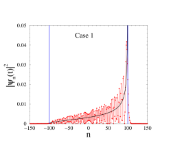
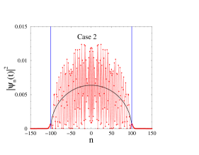
Figure 2: Probability profiles $|\psi_{n}(t)|^{2}$ at time $t=50$ for the simple quantum walk with the two exceptional initial states described in the text. Vertical blue lines: theoretical positions of the ballistic fronts. Black curves: asymptotic distributions (2.23), (2.25) set to scale.

2.2 Generalized quantum walk

Novel phenomena occur in generalized quantum walks, where the particle may hop to further neighbors. Let us consider the minimal generalization where hops are limited to first (nearest) and second (next-nearest) neighbors, with respective amplitudes 1 and $g$. The wavefunction of the particle at site $n$ at time $t$ now obeys

$${\rm i}\,{\frac{{\rm d}\psi_{n}(t)}{{\rm d}t}}=\psi_{n+1}(t)+\psi_{n-1}(t)+g\left(\psi_{n+2}(t)+\psi_{n-2}(t)\right).$$ (2.26)

We have therefore

$$\omega(q) = 2(\cos q+g\cos 2q),$$

$$\omega^{\prime}(q) = v(q)=-2(\sin q+2g\sin 2q),$$

$$\omega^{\prime\prime}(q) = -2(\cos q+4g\cos 2q).$$ (2.27)

The above dispersion law $\omega(q)$ is invariant under the transformation $g\to-g$, $q\to q+\pi$, $\omega\to-\omega$. We may therefore restrict the analysis to the domain $g\geq 0$, without any loss of generality.

Suppose the particle is launched from the origin: $\psi_{n}(0)=\delta_{n,0}$. Thus $\widehat{\psi}(q,0)=1$, and so

$$\psi_{n}(t)=\int_{0}^{2\pi}\frac{{\rm d}q}{2\pi}\,\rme^{{\rm i}(nq-\omega(q)t)}.$$ (2.28)

Some observables have a smooth dependence on the amplitude $g$. This is especially the case for the position moments (see (2.20)), which read

$$\langle n^{2}(t)\rangle = 2(1+4g^{2})t^{2},$$

$$\langle n^{4}(t)\rangle = 2(1+16g^{2})t^{2}+6(1+16g^{2}+16g^{4})t^{4},$$ (2.29)

and so on (odd moments vanish identically by symmetry).

The presence of hopping to second neighbors however introduces a novel qualitative feature. Let us for the time being adopt a general standpoint, and consider the wavefunction (2.28) in the regime of long times. Evaluating the integral by the saddle-point method, as we did in section 2.1, we obtain

$$\psi_{n}(t)\approx\sum_{q}\frac{\rme^{{\rm i}(nq-\omega(q)t)}}{\sqrt{2\pi{\rm i}\omega^{\prime\prime}(q)t}},$$ (2.30)

where the sum runs over the solutions $q$ of the saddle-point equation

$$\frac{n}{t}=v=\omega^{\prime}(q).$$ (2.31)

By averaging out the oscillations in the probabilities $|\psi_{n}(t)|^{2}$, we again predict that $v$ has a smooth distribution

$$f(v)=\frac{1}{2\pi}\sum_{q}\frac{1}{|\omega^{\prime\prime}(q)|}$$ (2.32)

in the long-time limit. In full generality, the above distribution is again obtained by folding the uniform distribution on the Brillouin zone by the dispersion map of the group velocity $v=\omega^{\prime}(q)$, in the sense that ${\rm d}q/(2\pi)=f(v){\rm d}v$ holds formally.

The distribution (2.32) has generically inverse-square-root singularities at all extremal values of $v$, in correspondence with wavevectors $q$ so that ${\rm d}v/{\rm d}q=\omega^{\prime\prime}(q)$ vanishes. It is always singular at the endpoints of the allowed region ($v=\pm V$), as the maximal velocity $V$ is necessarily an extremal value. The distribution (2.32) may however also have internal singularities within the allowed region, which were absent in the simple quantum walk considered in section 2.1.

Internal ballistic fronts of that kind have been observed in two generalizations of the usual discrete-time quantum walk [31, 34]. Reference [31] investigates a quantum walk subjected to $M$ independent quantum coins acting cyclically. If $M$ is large, the dynamics exhibits a crossover between classical random walk at short times ($t\ll M$) and quantum walk at long times ($t\gg M$). In the latter regime the distribution of the quantum particle exhibits an array of equally spaced ballistic peaks, whose number grows as $M/2$, the distance between any two consecutive peaks being $\Delta v=\sqrt{2}/M$. The model studied in [34] is closer to ours in its spirit. It consists of a discrete-time quantum walk where hops up to distance $j$ are allowed, whose dynamics is rigidly dictated by $(2j+1)$-dimensional Wigner rotation matrices. Here too, the distribution profile exhibits $2j+1$ equally spaced ballistic peaks.

In order to pursue the analysis, let us specialize to the continuous-time quantum walk with hops to first and second neighbors only (see (2.26), (2.27)). This minimal example is already too complex to allow one to turn (2.32) to an explicit expression. The location of the ballistic peaks can nevertheless be predicted as follows. The second derivative $\omega^{\prime\prime}(q)$ vanishes for

$$\cos q_{\pm}=\frac{-1\pm(1+128g^{2})^{1/2}}{16g}.$$ (2.33)

The corresponding values $V_{\pm}$ of $v$ are given by

$$V_{\pm}^{2}=\frac{-1+320g^{2}+2048g^{4}\pm(1+128g^{2})^{3/2}}{128g^{2}}.$$ (2.34)

The allowed region always spreads ballistically with the maximal velocity $V_{+}$. The smaller velocity $V_{-}$ may also play a role, depending on the strength of $g$:

• If the amplitude $g$ is small enough ($g<g_{c}=1/4$), the situation is qualitatively similar to that of the simple quantum walk, studied in section 2.1. We have indeed $\cos q_{-}<-1$ and $0<\cos q_{+}<1$, so that only $q_{+}$ matters, and so $f(v)$ is only singular at the endpoints $\pm V_{+}$ of the allowed region.

• If the amplitude $g$ is large enough ($g>g_{c}=1/4$), both $q_{+}$ and $q_{-}$ matter. As a consequence, the distribution $f(v)$ has two singularities at the endpoints $\pm V_{+}$ and two internal singularities at the smaller values $\pm V_{-}$. The wavefunction exhibits four ballistic fronts: two extremal ones, propagating at the maximal velocity ($\pm V_{+}$), and two internal ones, propagating at a smaller velocity ($\pm V_{-}$).

• In the borderline case ($g=g_{c}=1/4$), we have $\cos q_{-}=-1$, i.e., $q_{-}=\pi$ and $V_{-}=0$. The dispersion curve exhibits an unusual quartic behavior near $q=\pi$:

  $$\omega(q)\approx-\frac{3}{2}+\frac{\varepsilon^{4}}{4}\qquad(\varepsilon=q-\pi\to 0).$$ (2.35)

  This anomalous dispersion right at $g=g_{c}$ has two consequences. First, the distribution $f(v)$ has a singularity at $v=0$, of the form

  $$f(v)\approx\frac{1}{6\pi|v|^{2/3}}.$$ (2.36)

  This central singularity with exponent $-2/3$ is stronger than the generic ones, whose exponent is $-1/2$. Second, the wavefunction at the origin exhibits an unusually slow fall-off:

  $$\psi_{0}(t)\approx\frac{\sqrt{2}\,\Gamma(5/4)\,\rme^{{\rm i}(3t/2-\pi/8)}}{\pi t^{1/4}}.$$ (2.37)

  This $t^{-1/4}$ decay is slower than the generic $t^{-1/2}$ decay exhibited e.g. by the Bessel function $J_{0}(2t)$ (see (2.3)).

Figure 3 shows the dependence of the front velocities against $g$ for $g\geq 0$. The larger velocities $\pm V_{+}$ of the extremal fronts (blue curves) describe the endpoints of the allowed region for all $g$. The smaller velocities $\pm V_{-}$ of the internal fronts (red curves) exist for $g>g_{c}=1/4$ only. At $g=g_{c}$ we have $V_{+}=3\sqrt{3}/2$, while $V_{-}$ takes off as $(32\sqrt{6}/9)(g-g_{c})^{3/2}$. At large $g$, both velocities grow linearly in $g$ with the same slope, as $V_{\pm}\approx 4g\pm\sqrt{2}$. This non-trivial pattern of front velocities is richer than the periodic arrays of equally spaced peaks observed in [31, 34].

Figure 4 shows the probabilities $|\psi_{n}(t)|^{2}$ at time $t=50$ for a particle launched at the origin and two values of $g$. For $g=1/2$ (left), the probability profile exhibits four fronts. For $g=g_{c}=1/4$ (right), the probability profile exhibits three fronts. The central one at the origin corresponds to the anomalous singularity (2.36).

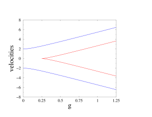
Figure 3: Front velocities of the quantum walk with hopping to first and second neighbors (see (2.26)), against the amplitude $g$. External (blue) curves: velocities $\pm V_{+}$ of the extremal fronts (endpoints of allowed region). Internal (red) curves: velocities $\pm V_{-}$ of the internal fronts for $g>g_{c}=1/4$.

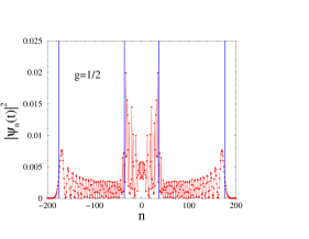
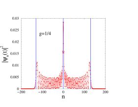
Figure 4: Probabilities $|\psi_{n}(t)|^{2}$ for the quantum walk (2.26) at time $t=50$. Vertical blue lines: theoretical positions of the ballistic fronts. Left ($g=1/2$): four fronts at $\pm V_{+}$ and $\pm V_{-}$. Right ($g=g_{c}=1/4$): two fronts at $\pm V_{+}$ and a central one at the origin, corresponding to the anomalous power-law singularity (2.36).

3 Two-body bound states: hard bound on distance

We now turn to our main subject: the quantum walk performed by a bound state of two identical particles propagating coherently along a one-dimensional lattice. The main emphasis will be on the asymptotic distribution of the center-of-mass coordinate of the bound state, on the velocity characterizing its ballistic spreading and on the structure of the distribution profile, which generically exhibits many internal fronts. To the best of our knowledge, these matters have only been addressed so far in two papers [21, 25]. In order not to interrupt the lengthy developments of sections 3 and 4, we postpone the discussion of those earlier works to section 5.

Here again, considering continuous-time walks will allow for a more thorough and systematic investigation of the problem. Bound states obtained by imposing a hard bound $\ell$ on the distance between both particles are dealt with in this section, whereas those generated by a smooth confining potential will be considered in section 4. The same formalism will allow one to deal with bosonic and fermionic bound states, as they are respectively described by even and odd functions of the relative coordinate $m$ between both particles.

3.1 Generalities

We denote by $n_{1}=n+m$ and $n_{2}=n$ the abscissas of two identical particles on the lattice, where $m=n_{1}-n_{2}$ is the relative coordinate. We impose a hard bound $\ell$ on the distance $|m|$ between both particles, and so $m$ is restricted to the $2\ell+1$ values $m=-\ell,\dots,\ell$. Figure 5 shows the positions of the particles in the $(n_{1},n_{2})$ plane for $\ell=2$. Full symbols denote the allowed configurations of the particles. Links between symbols show the allowed hops of any of the particles to a neighboring site.

Figure 5: Plot of the positions of the particles in the $(n_{1},n_{2})$ plane for $\ell=2$. Full symbols denote the allowed configurations of the particles. Links between symbols show the allowed hops of any of the particles to a neighboring site.

The time-dependent wavefunction

$$\psi_{n,m}(t)=\langle(n_{1},n_{2})|\psi(t)\rangle=\langle(n+m,n)|\psi(t)\rangle$$ (3.1)

obeys the equation

$${\rm i}\,{\frac{{\rm d}\psi_{n,m}(t)}{{\rm d}t}} = \psi_{n,m-1}(t)+\psi_{n+1,m-1}(t)$$ (3.2)

$$+ \psi_{n-1,m+1}(t)+\psi_{n,m+1}(t),$$

with boundary conditions $\psi_{n,\pm(\ell+1)}=0$.

3.2 Bosonic and fermionic spectra

A basis of plane-wave solutions to (3.2) reads

$$\psi_{n,m}(t)=\rme^{{\rm i}(n_{\rm cm}q+mp-\omega(p,q)t)},$$ (3.3)

where the momenta $p$ and $q$ are respectively conjugate to the relative coordinate $m=n_{1}-n_{2}$ and to the center-of-mass coordinate

$$n_{\rm cm}=\frac{n_{1}+n_{2}}{2}=n+\frac{m}{2}.$$ (3.4)

The resulting dispersion relation has a product form [25]:

$$\omega(p,q)=4\cos p\cos\frac{q}{2}.$$ (3.5)

• Bosonic states are described by even functions under the exchange of $n_{1}$ and $n_{2}$; they are obtained by adding the plane waves (3.3) for $p$ and $-p$:

  $$\psi_{n,m}^{(\rm B)}(t)=\rme^{{\rm i}(n_{\rm cm}q-\omega(p,q)t)}\cos mp.$$ (3.6)

  The relative momentum $p$ is quantized by the condition $\cos(\ell+1)p=0$. It therefore takes the $\ell+1$ values

  $$p_{k}^{(\rm B)}=\frac{(k+\frac{1}{2})\pi}{\ell+1}\qquad(k=0,\dots,\ell),$$ (3.7)

  and so

  $$\omega_{k}^{(\rm B)}(q)=4\cos\frac{(k+\frac{1}{2})\pi}{\ell+1}\,\cos\frac{q}{2}.$$ (3.8)

  The bosonic dispersion curve thus consists of $\ell+1$ branches, with group velocities

  $$v_{k}^{(\rm B)}(q)=-2\cos\frac{(k+\frac{1}{2})\pi}{\ell+1}\,\sin\frac{q}{2}.$$ (3.9)

• Fermionic states are described by odd functions of $m$, obtained by subtracting the plane waves (3.3) for $p$ and $-p$:

  $$\psi_{n,m}^{(\rm F)}(t)=\rme^{{\rm i}(n_{\rm cm}q-\omega(p,q)t)}\sin mp.$$ (3.10)

  As fermionic particles cannot cross each other in one dimension, the range of the fermionic wavefunctions (3.10) can be restricted to the sector $n_{1}>n_{2}$, i.e., $m=1,\dots,\ell$. The relative momentum $p$ is quantized by the condition $\sin(\ell+1)p=0$. It therefore takes the $\ell$ values

  $$p_{k}^{(\rm F)}=\frac{k\pi}{\ell+1}\qquad(k=1,\dots,\ell),$$ (3.11)

  and so

  $$\omega_{k}^{(\rm F)}(q)=4\cos\frac{k\pi}{\ell+1}\,\cos\frac{q}{2}.$$ (3.12)

  The fermionic dispersion curve thus consists of $\ell$ branches, with group velocities

  $$v_{k}^{(\rm F)}(q)=-2\cos\frac{k\pi}{\ell+1}\,\sin\frac{q}{2}.$$ (3.13)

Figure 6 shows the bosonic and fermionic spectra for a maximal distance $\ell=6$. The 7 bosonic frequencies $\omega_{k}^{(\rm B)}(q)$ (black) and the 6 fermionic frequencies $\omega_{k}^{(\rm F)}(q)$ (red) are plotted against $q/\pi$.

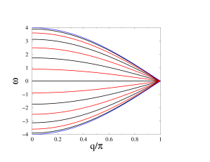
Figure 6: Plot of the bosonic and fermionic spectra for a maximal distance $\ell=6$, against $q/\pi$. Black: bosonic frequencies $\omega_{k}^{(\rm B)}(q)$. Red: fermionic frequencies $\omega_{k}^{(\rm F)}(q)$. Blue: band boundaries ($\omega=\pm 4\cos(q/2)$) (see (3.5)).

3.3 Ballistic spreading

Let us now investigate the asymptotic behavior of the wavefunction $\psi_{n,m}(t)$, starting from an arbitrary initial state, where both particles are located in the vicinity of the origin. The detailed analysis of the one-body problem performed in section 2 allows one to draw the following picture.

The various components $\psi_{n,m}(t)$ of the wavefunction spread ballistically, i.e., their extension in the center-of-mass coordinate $n_{\rm cm}\approx n$ grows asymptotically linearly in time $t$ and symmetrically with respect to the origin. The $\psi_{n,m}(t)$ generically exhibit sharp fronts near $n=V_{k}t$, where the front velocities $V_{k}$ are the stationary values of the group velocity, corresponding to the boundaries of the Brillouin zone. Setting $q=\pm\pi$ in (3.9), (3.13), we get

$$V_{k}^{(\rm B)} = 2\cos\frac{(k+\frac{1}{2})\pi}{\ell+1}\qquad(k=0,\dots,\ell),$$

$$V_{k}^{(\rm F)} = 2\cos\frac{k\pi}{\ell+1}\qquad(k=1,\dots,\ell).$$ (3.14)

In particular, all the components of the wavefunction take appreciable values only in the allowed zone defined by $|n|<Vt$, where the maximal velocities

$$V^{(\rm B)}=2\cos\frac{\pi}{2(\ell+1)},\qquad V^{(\rm F)}=2\cos\frac{\pi}{\ell+1},$$ (3.15)

respectively correspond to setting $k=0$ and $k=1$ in (3.14). Both maximal velocities approach the free value $V=2$ in the limit of a large confining size ($\ell\gg 1$), with two different correction amplitudes, i.e.,

$$V^{(\rm B)}\approx 2-\frac{C^{(\rm B)}}{\ell^{2}},\qquad V^{(\rm F)}\approx 2-\frac{C^{(\rm F)}}{\ell^{2}},$$ (3.16)

$$C^{(\rm B)}=\frac{\pi^{2}}{4},\qquad C^{(\rm F)}=\pi^{2}.$$ (3.17)

For a generic initial state localized in the vicinity of the origin, the various components $\psi_{n,m}(t)$ of the wavefunction will exhibit, besides two extremal ballistic fronts at $n=\pm V^{(\rm B)}t$ or $n=\pm V^{(\rm F)}t$, $\ell-1$ internal fronts in the bosonic case (for $\ell\geq 2$) and $\ell-2$ internal fronts in the fermionic case (for $\ell\geq 3$).

3.4 Continuum limit and corrections

Our bound-state problem owes its non-triviality and its richness to the fact that particles live on a lattice. In the continuum limit, the dynamics of the center-of-mass coordinate and of the relative coordinate are exactly decoupled, as a consequence of Galilean invariance. As soon as the line is discretized into a lattice, this Galilean invariance is broken. This phenomenon has already been underlined for discrete-time interacting quantum walkers [21]. Its consequences in the context of diluted Fermi gases and of the BCS–BEC crossover have also been discussed recently [42].

In the present situation, too, the dynamics of the center-of-mass coordinate $n_{\rm cm}$ and of the relative coordinate $m$ are expected to decouple as the continuum limit is approached, where Galilean invariance should be restored. It is worth investigating in a quantitative way how this decoupling takes place, starting from the lattice dispersion curves (3.8) and (3.12). For that purpose, we introduce the lattice spacing $a$, and define the following dimensionful quantities, denoted by capital letters. The half-width of the potential well is conveniently defined as $L=(\ell+1)a$, while the conjugate momentum to the center-of-mass coordinate is $Q=q/a$, and finally the continuum energy reads $E=(4-\omega)/(2a^{2})$.

To leading order as $a\to 0$ (i.e., in the vicinity of the center of the Brillouin zone), both dispersion relations (3.8) and (3.12) yield

$$E_{k}\approx\frac{Q^{2}}{4}+\varepsilon_{k},$$ (3.18)

where the $\varepsilon_{k}$ are the energy levels of a free particle in a potential well of width $2L$ in the appropriate sectors, i.e.,

$$\varepsilon_{k}^{(\rm B)}=\left(\frac{(k+\frac{1}{2})\pi}{L}\right)^{2},\qquad\varepsilon_{k}^{(\rm F)}=\left(\frac{k\pi}{L}\right)^{2}.$$ (3.19)

The expression (3.18) conforms to what we expect from the continuum theory: the total energy $E_{k}$ of the compound system is the sum of the kinetic energy $Q^{2}/4$ of the center-of-mass motion and of the energy $\varepsilon_{k}$ of a bound state in the relative coordinate.

The corrections to the leading-order result (3.18) can be derived by recasting (3.8) and (3.12) in terms of the dimensionful quantities introduced above, and expanding in powers of $a$. The first correction thus obtained,

$$E_{k}=\frac{Q^{2}}{4}+\varepsilon_{k}-\left(Q^{4}+24Q^{2}\varepsilon_{k}+16\varepsilon_{k}^{2}\right)\frac{a^{2}}{192}+\cdots,$$ (3.20)

already demonstrates that the coupling of both degrees of freedom by the lattice structure affects the energy spectrum in a non-trivial way.

3.5 A case study: fermionic state with maximal distance $\ell=4$

To close this section, let us investigate in detail the dynamics of a fermionic bound state with maximal distance $\ell=4$. This is the smallest $\ell$ for which generic dynamical behavior is observed. The front velocities (3.14) read

$$V_{1}^{(\rm F)} = -V_{4}^{(\rm F)}=2\cos\frac{\pi}{5}=\tau=\frac{\sqrt{5}+1}{2},$$

$$V_{2}^{(\rm F)} = -V_{3}^{(\rm F)}=2\cos\frac{2\pi}{5}={\widetilde{\tau}}=\frac{\sqrt{5}-1}{2},$$ (3.21)

where $\tau$ is the golden mean and ${\widetilde{\tau}}$ its reciprocal.

Suppose the two fermions are launched from sites 0 and 1 at time $t=0$. Then $\psi_{n,m}(0)=\delta_{n,0}\delta_{m,1}$ and the initial mean value of the center-of-mass coordinate is $\langle n_{\rm cm}(0)\rangle=\langle\psi(0)|n_{\rm cm}|\psi(0)\rangle=1/2$. We expect there will be two extremal ballistic fronts near $n=\pm\tau t$, and two internal ones near $n=\pm{\widetilde{\tau}}t$.

The most efficient way of solving the differential equations (3.1) with prescribed initial values consists in performing a spatial Fourier transform (with $q$ being conjugate to $n$) and a temporal Laplace transform (with $s$ being conjugate to $t$). The Fourier-Laplace transforms thus defined obey the equations

$${\rm i}s\widehat{\psi}_{1}(q,s)=(\rme^{-{\rm i}q}+1)\widehat{\psi}_{2}(q,s)+{\rm i},$$

$${\rm i}s\widehat{\psi}_{2}(q,s)=(\rme^{{\rm i}q}+1)\widehat{\psi}_{1}(q,s)+(\rme^{-{\rm i}q}+1)\widehat{\psi}_{3}(q,s),$$

$${\rm i}s\widehat{\psi}_{3}(q,s)=(\rme^{{\rm i}q}+1)\widehat{\psi}_{2}(q,s)+(\rme^{-{\rm i}q}+1)\widehat{\psi}_{4}(q,s),$$

$${\rm i}s\widehat{\psi}_{4}(q,s)=(\rme^{{\rm i}q}+1)\widehat{\psi}_{3}(q,s).$$ (3.22)

This linear system can be readily solved. Introducing the notation

$$\gamma=2\cos\frac{q}{2},$$ (3.23)

we obtain

$$\widehat{\psi}_{1}(q,s)=\frac{s(s^{2}+2\gamma^{2})}{\Delta(q,s)},\qquad\widehat{\psi}_{2}(q,s)=-{\rm i}\frac{(\rme^{{\rm i}q}+1)(s^{2}+\gamma^{2})}{\Delta(q,s)},$$

$$\widehat{\psi}_{3}(q,s)=-\frac{(\rme^{{\rm i}q}+1)^{2}s}{\Delta(q,s)},\qquad\widehat{\psi}_{4}(q,s)={\rm i}\frac{(\rme^{{\rm i}q}+1)^{3}}{\Delta(q,s)},$$ (3.24)

with

$$\Delta(q,s)=(s-{\rm i}\gamma\tau)(s-{\rm i}\gamma{\widetilde{\tau}})(s+{\rm i}\gamma\tau)(s+{\rm i}\gamma{\widetilde{\tau}}).$$ (3.25)

The inverse Laplace transform of (3.24) can be taken first. We have e.g.

$$\widehat{\psi}_{1}(q,s)=\frac{1}{2\sqrt{5}}\left(\frac{{\widetilde{\tau}}}{s-{\rm i}\gamma\tau}+\frac{{\widetilde{\tau}}}{s+{\rm i}\gamma\tau}+\frac{\tau}{s-{\rm i}\gamma{\widetilde{\tau}}}+\frac{\tau}{s+{\rm i}\gamma{\widetilde{\tau}}}\right),$$ (3.26)

and so

$$\widehat{\psi}_{1}(q,t)=\frac{1}{2\sqrt{5}}\left({\widetilde{\tau}}\rme^{{\rm i}\gamma\tau t}+{\widetilde{\tau}}\rme^{-{\rm i}\gamma\tau t}+\tau\rme^{{\rm i}\gamma{\widetilde{\tau}}t}+\tau\rme^{-{\rm i}\gamma{\widetilde{\tau}}t}\right).$$ (3.27)

The inverse Fourier transform can then be taken using (see (2.3))

$$\int_{0}^{2\pi}\frac{{\rm d}q}{2\pi}\,\rme^{{\rm i}(nq+x\cos(q/2))}=(-1)^{n}J_{2n}(x),$$

$$\int_{0}^{2\pi}\frac{{\rm d}q}{2\pi}\,\rme^{{\rm i}((n+1/2)q+x\cos(q/2))}={\rm i}(-1)^{n}J_{2n+1}(x).$$ (3.28)

We thus obtain

$$\psi_{n,1}(t) = \frac{(-1)^{n}}{\sqrt{5}}\bigl{(}{\widetilde{\tau}}J_{2n}(2\tau t)+\tau J_{2n}(2{\widetilde{\tau}}t)\bigr{)},$$

$$\psi_{n,2}(t) = {\rm i}\frac{(-1)^{n+1}}{\sqrt{5}}\bigl{(}J_{2n+1}(2\tau t)+J_{2n+1}(2{\widetilde{\tau}}t)\bigr{)},$$

$$\psi_{n,3}(t) = \frac{(-1)^{n+1}}{\sqrt{5}}\bigl{(}J_{2n+2}(2\tau t)-J_{2n+2}(2{\widetilde{\tau}}t)\bigr{)},$$

$$\psi_{n,4}(t) = {\rm i}\frac{(-1)^{n}}{\sqrt{5}}\bigl{(}{\widetilde{\tau}}J_{2n+3}(2\tau t)-\tau J_{2n+3}(2{\widetilde{\tau}}t)\bigr{)}.$$ (3.29)

Figure 7 shows the four probability profiles $|\psi_{n,m}(t)|^{2}$ thus obtained at time $t=50$. Abscissas are shifted from $n$ to $n+(m-1)/2=n_{\rm cm}-\langle n_{\rm cm}(0)\rangle$, in such a way that the plotted profiles are exactly symmetric. The four profiles exhibit the same global features, although they differ in their detailed structure. As predicted, they exhibit the same ballistic fronts, two external ones at $n\approx\pm\tau t$ and two internal ones at $n\approx\pm{\widetilde{\tau}}t$ (see (3.21)). The probabilities are larger within the internal fronts, and considerably smaller in the wings of the allowed zone, i.e., between the internal and the external fronts. This phenomenon is quite generic; it could already be observed in the left panel of figure 4.

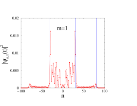
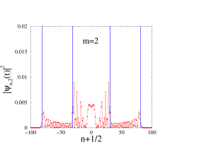
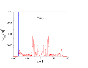
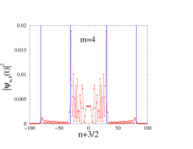
Figure 7: Probability profiles $|\psi_{n,m}(t)|^{2}$ ($m=1$ to 4) of the fermionic bound state with maximal distance $\ell=4$ at time $t=50$, with initial state $\psi_{n,m}(0)=\delta_{n,0}\delta_{m,1}$, against $n+(m-1)/2=n_{\rm cm}-\langle n_{\rm cm}(0)\rangle$. Vertical blue lines: theoretical positions of the ballistic fronts.

Let us now turn to the internal structure of the fermionic bound state. The distance between both particles takes the value $m=1,\dots,4$ with probability

$$P_{m}(t)=\sum_{n}|\psi_{n,m}(t)|^{2}.$$ (3.30)

These probabilities can be evaluated from (3.29) using identities

$$\sum_{n}J_{2n}(x)J_{2n}(y)=\frac{J_{0}(x-y)+J_{0}(x+y)}{2},$$

$$\sum_{n}J_{2n+1}(x)J_{2n+1}(y)=\frac{J_{0}(x-y)-J_{0}(x+y)}{2},$$ (3.31)

which can be derived from the integral representations (3.28). Quadratic identities of this kind have their roots in the connection between special functions and representation theory [43]. We thus obtain

$$P_{1}(t)=\frac{1}{10}\bigl{(}3+{\widetilde{\tau}}^{2}J_{0}(4\tau t)+\tau^{2}J_{0}(4{\widetilde{\tau}}t)+2J_{0}(2t)+2J_{0}(2\sqrt{5}t)\bigr{)},$$

$$P_{2}(t)=\frac{1}{10}\bigl{(}2-J_{0}(4\tau t)-J_{0}(4{\widetilde{\tau}}t)+2J_{0}(2t)-2J_{0}(2\sqrt{5}t)\bigr{)},$$

$$P_{3}(t)=\frac{1}{10}\bigl{(}2+J_{0}(4\tau t)+J_{0}(4{\widetilde{\tau}}t)-2J_{0}(2t)-2J_{0}(2\sqrt{5}t)\bigr{)},$$

$$P_{4}(t)=\frac{1}{10}\bigl{(}3-{\widetilde{\tau}}^{2}J_{0}(4\tau t)-\tau^{2}J_{0}(4{\widetilde{\tau}}t)-2J_{0}(2t)+2J_{0}(2\sqrt{5}t)\bigr{)}.$$ (3.32)

These probabilities sum up to unity, as should be. They are even functions of $t$ whose power series have rational coefficients. At short times we have

$$P_{1}(t)=1-2t^{2}+\frac{5t^{4}}{2}-\frac{35t^{6}}{18}\cdots,$$

$$P_{2}(t)=2t^{2}-4t^{4}+\frac{35t^{6}}{9}+\cdots,$$

$$P_{3}(t)=\frac{3t^{4}}{2}-\frac{5t^{6}}{2}+\cdots,$$

$$P_{4}(t)=\frac{5t^{6}}{9}+\cdots$$ (3.33)

In the long-time regime, these probabilities reach the stationary values

$$P_{1}=P_{4}=\frac{3}{10},\qquad P_{2}=P_{3}=\frac{1}{5}.$$ (3.34)

These numbers agree with the result (1.14) derived in A. In the present situation, it is indeed legitimate to study the stationary properties of the internal state per se, without referring to the ballistic dynamics of the center-of-mass coordinate, because the compound system has a basis of factorized eigenstates (3.3). This feature is by no means general.

Figure 8 shows a plot of the probabilities $P_{m}(t)$ against time $t$. The maximal time $t=50$ corresponds to the profiles shown in figure 7. The stationary values (3.34) (arrows) are reached after a complex pattern of damped oscillations. The envelope of this transient oscillatory behavior falls off very slowly as $t^{-1/2}$, while the oscillations themselves follow a quasiperiodic pattern, characterized by the two incommensurate frequencies $2\tau$ and $2{\widetilde{\tau}}$. All the frequencies entering (3.32) are indeed integer linear combinations of the latter frequencies. In a generic situation, there will be as many incommensurate frequencies as there are positive ballistic velocities $V_{k}^{(\rm B)}$ or $V_{k}^{(\rm F)}$ (see (3.14)).

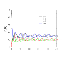
Figure 8: Probabilities $P_{m}(t)$ describing the internal structure of the fermionic bound state (see text) against time $t$. Arrows: stationary values (3.34).

The mean internal size of the bound state,

$$D(t)=\sum_{m=1}^{4}mP_{m}(t),$$ (3.35)

can be evaluated from (3.32) to read

$$D(t)=\frac{1}{10}\bigl{(}25-(2-3{\widetilde{\tau}})J_{0}(4\tau t)-(2+3\tau)J_{0}(4{\widetilde{\tau}}t)-8J_{0}(2t)\bigr{)}.$$ (3.36)

This quantity is plotted in figure 9. It starts from $D(0)=1$ and reaches the stationary value $D=5/2$, again after a complex pattern of quasiperiodic oscillations dying off as $t^{-1/2}$.

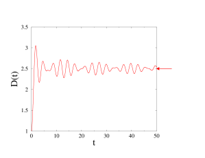
Figure 9: Plot of the mean internal size $D(t)$ of the fermionic bound state against time $t$. Arrow: stationary value ($D=5/2$).

4 Two-body bound states: smooth confining potential

4.1 Generalities

We now turn to the quantum walk performed by a bosonic or fermionic bound state of two identical particles generated by a smooth confining potential $W_{m}$. The latter is assumed to be an even function of the relative coordinate $m$ between both particles, such that $W_{m}\to+\infty$ at large distances ($|m|\to\infty$). With the notations of section 3, the time-dependent wavefunction $\psi_{n,m}(t)$ obeys the equation

$${\rm i}\,{\frac{{\rm d}\psi_{n,m}(t)}{{\rm d}t}}=W_{m}\psi_{n,m}(t) + \psi_{n,m-1}(t)+\psi_{n+1,m-1}(t)$$ (4.1)

$$+ \psi_{n-1,m+1}(t)+\psi_{n,m+1}(t).$$

Let us look for a basis of solutions to (4.1) of the form (see (3.3))

$$\psi_{n,m}(t)=\rme^{{\rm i}(n_{\rm cm}q-\omega t)}\phi_{m},$$ (4.2)

where the momentum $q$ is conjugate to the center-of-mass coordinate (3.4). The internal wavefunction $\phi_{m}$ obeys

$$\omega\phi_{m}=\gamma(\phi_{m-1}+\phi_{m+1})+W_{m}\phi_{m},$$ (4.3)

with the same dispersive (i.e., $q$-dependent) hopping amplitude

$$\gamma=2\cos\frac{q}{2}$$ (4.4)

as before (see (3.23)). We shall also use the shorthand notation

$$\chi_{m}=(-1)^{m}\phi_{m},$$ (4.5)

for the staggered wavefunction, which obeys

$$\omega\chi_{m}=-\gamma(\chi_{m-1}+\chi_{m+1})+W_{m}\chi_{m},$$ (4.6)

i.e., (4.3) with the sign of $\gamma$ reversed.

The above formalism applies to an arbitrary confining potential. Bosonic and fermionic bound states are described by wavefunctions $\phi_{m}$ which are respectively even and odd functions of $m$, such that $\phi_{m}\to 0$ at large distances. Such bound-state wavefunctions only exist for discrete sequences of dispersive frequencies $\omega_{k}^{(\rm B)}(q)$ and $\omega_{k}^{(\rm F)}(q)$. Hereafter we investigate in detail the case of potentials growing as a power of distance, either linearly (section 4.2), quadratically (section 4.3), or as an arbitrary power (section 4.4).

4.2 Linear confining potential

Our first example is the linear confining potential

$$W_{m}=g|m|,$$ (4.7)

where the amplitude $g$ is a positive constant. The regime of most physical interest corresponds to small $g$, so that bound states have a large size and potentially a rich internal structure.

Figure 10 shows the bosonic and fermionic spectra for $g=0.4$. These spectra exhibit two very distinct regions. Within the band delimited by the blue curves ($\omega=\pm 2\gamma=\pm 4\cos(q/2)$), bosonic and fermionic branches are well separated from each other. They alternate and are strongly dispersive. Above the band, the spectrum consists of an infinite array of approximately equally spaced and non-dispersive branches. These branches appear as red, as bosonic and fermionic branches are superimposed to a very high accuracy.

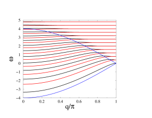
Figure 10: Plot of the bosonic and fermionic spectra for the linear confining potential with $g=0.4$, against $q/\pi$. Black: bosonic frequencies $\omega_{k}^{(\rm B)}(q)$. Red: fermionic frequencies $\omega_{k}^{(\rm F)}(q)$. Blue: band boundaries ($\omega=\pm 2\gamma=\pm 4\cos(q/2)$).

In order to analyze the above observations, we use (4.6) for positive values of the relative coordinate $m$, i.e.,

$$\omega\chi_{m}=-\gamma(\chi_{m-1}+\chi_{m+1})+gm\chi_{m}\qquad(m\geq 0).$$ (4.8)

Let us first forget about the constraint $m\geq 0$ and extend (4.8) to all values of $m$. We are thus facing a tight-binding equation for a charged particle in a uniform electric field, the amplitude $g$ giving the strength of the field in reduced units. The corresponding spectrum is a Wannier-Stark ladder [44, 45]: it consists of the infinite sequence of equally spaced frequencies,

$$\omega_{k}=gk,$$ (4.9)

where $k$ runs over the integers. The Wannier-Stark levels are non-dispersive, as (4.9) holds irrespective of the hopping amplitude $\gamma$. The normalized eigenfunction corresponding to $\omega_{k}$ reads

$$\chi_{m}=J_{m-k}(2\gamma/g),$$ (4.10)

where the $J_{m}$ are the Bessel functions. This eigenfunction is strongly localized around $m=k$. We have in particular, for large positive $k$,

$$|\chi_{0}|\approx\frac{(\gamma/g)^{k}}{k!}\sim\left(\frac{\rme\gamma}{gk}\right)^{k}.$$ (4.11)

This estimate shows that the Wannier-Stark eigenfunctions hardly feel the boundary condition on (4.8) at $m=0$, and therefore remain essentially unperturbed, as soon as the frequency $\omega_{k}=gk$ exceeds a few times the bandwidth $\gamma$. In other words, only finitely many lowest Wannier-Stark states, in a number of the order of $\gamma/g$, are affected by the boundary condition which distinguishes between fermions and bosons. This explains the main observations made on figure 10.

A more quantitative analysis of the problem goes as follows. The general solution to (4.8) falling off as $m\to+\infty$ reads

$$\chi_{m}=J_{m-\omega/g}(2\gamma/g)\qquad(m\geq-1),$$ (4.12)

where the $J_{\nu}(z)$ are the Bessel functions with index $\nu$, which obey the identities

$$J_{\nu-1}(z)+J_{\nu+1}(z) = \frac{2\nu}{z}\,J_{\nu}(z),$$

$$J_{\nu-1}(z)-J_{\nu+1}(z) = 2J^{\prime}_{\nu}(z),$$ (4.13)

where the prime denotes a derivative with respect to $z$. The bosonic spectrum is given by $\chi_{1}=\chi_{-1}$, while for the fermionic spectrum $\chi_{0}=0$. We thus arrive at the exact quantization formulas

$$J^{\prime}_{-\omega^{(\rm B)}/g}(2\gamma/g)=0,\qquad J_{-\omega^{(\rm F)}/g}(2\gamma/g)=0.$$ (4.14)

The leading correction to the Wannier-Stark spectrum (4.9) at large positive $k$ can be readily derived from (4.14). Skipping details, we obtain a symmetric splitting of the form

$$\omega_{k}^{(\rm B)}\approx g(k+\varepsilon_{k}),\qquad\omega_{k}^{(\rm F)}\approx g(k-\varepsilon_{k}),$$ (4.15)

with

$$\varepsilon_{k}\approx\frac{(\gamma/g)^{2k}}{k!(k-1)!}\approx k\chi_{0}^{2},$$ (4.16)

where $\chi_{0}$ is the Wannier-Stark wavefunction at the origin (see (4.11)).

Our next goal is to investigate the velocities characterizing the ballistic spreading of a bosonic or fermionic wavefunction in the center-of-mass coordinate $n_{\rm cm}$, for a generic initial state. These velocities are given by

$$V^{(\rm B)}=\mathrel{\mathop{{\rm max}}\limits_{k,q}}|\omega_{k}^{\prime{(\rm B)}}(q)|,\qquad V^{(\rm F)}=\mathrel{\mathop{{\rm max}}\limits_{k,q}}|\omega_{k}^{\prime{(\rm F)}}(q)|,$$ (4.17)

where primes denote derivatives, and maxima are taken over all branches of the spectrum and over all $q$. It is clear from figure 10 that these maxima are reached for the lowest branch of each spectrum. Furthermore, if the amplitude $g$ is small, so that the bound states have a large internal size, we anticipate that the maximal velocities will be close to the free value 2 and correspond to momenta close to the zone boundary ($q\to\pi$).

To substantiate these expectations we note that whenever $g$ is small, typical wavefunctions vary slowly with $m$, so one can employ a continuum description. Setting

$$\omega=-2\gamma+\delta=-4\cos\frac{q}{2}+\delta,$$ (4.18)

and expanding in (4.8) differences in terms of derivatives, we obtain

$$\gamma\frac{{\rm d}^{2}\chi}{{\rm d}m^{2}}\approx(gm-\delta)\chi.$$ (4.19)

Then, setting

$$x=\lambda(gm-\delta),\qquad\lambda=(g^{2}\gamma)^{-1/3},$$ (4.20)

Equation (4.19) becomes the Airy equation

$$\frac{{\rm d}^{2}\chi}{{\rm d}x^{2}}=x\chi,$$ (4.21)

whose solution decaying as $x\to+\infty$ is $\chi(x)={\rm Ai}(x)$, the Airy function.

• Bosonic states obey $\chi_{1}=\chi_{-1}$, hence ${\rm d}\chi/{\rm d}m=0$ for $m=0$, and so $x_{0}=-\lambda\delta$ obeys ${\rm Ai}^{\prime}(x_{0})=0$. The lowest branch of the bosonic spectrum therefore reads

  $$\delta^{(\rm B)}\approx\eta_{1}(g^{2}\gamma)^{1/3},$$ (4.22)

  where $\eta_{1}=1.018792\dots$ is the opposite of the first zero of ${\rm Ai}^{\prime}(x)$.

  Setting $q=\pi-\varepsilon$, the lowest branch can be expanded as

  $$\omega=-4\sin\frac{\varepsilon}{2}+\delta=-2\varepsilon+\frac{\varepsilon^{3}}{12}+\cdots+\delta.$$ (4.23)

  Using the expression (4.22) of $\delta$, we can show that the maximal group velocity reads

  $$V^{(\rm B)}\approx 2-C^{(\rm B)}\,g^{1/2},$$ (4.24)

  $$C^{(\rm B)}=\left(\frac{4\eta_{1}}{9}\right)^{3/4}=0.551985\dots,$$ (4.25)

  and is reached for

  $$\varepsilon\approx(C^{(\rm B)})^{1/2}\,g^{1/4}.$$ (4.26)

• Fermionic states obey $\chi_{0}=0$, and so $x_{0}=-\lambda\delta$ obeys ${\rm Ai}(x_{0})=0$. The lowest branch of the fermionic spectrum therefore reads

  $$\delta^{(\rm F)}\approx\xi_{1}(g^{2}\gamma)^{1/3},$$ (4.27)

  where $\xi_{1}=2.338107\dots$ is the opposite of the first zero of ${\rm Ai}(x)$. The maximal group velocity now reads

  $$V^{(\rm F)}\approx 2-C^{(\rm F)}\,g^{1/2},$$ (4.28)

  $$C^{(\rm F)}=\left(\frac{4\xi_{1}}{9}\right)^{3/4}=1.029227\dots,$$ (4.29)

  and it is reached for

  $$\varepsilon\approx(C^{(\rm F)})^{1/2}\,g^{1/4}.$$ (4.30)

The above scaling results valid in the $g\ll 1$ regime can be alternatively derived by analyzing the exact quantization formulas (4.14) in the transition region (see (2.8)). We have in particular

$$\frac{C^{(\rm F)}}{C^{(\rm B)}}=\left(\frac{\xi_{1}}{\eta_{1}}\right)^{3/4}=1.864592\dots$$ (4.31)

Figure 11 shows plots of the maximal velocities $V^{(\rm B)}$ and $V^{(\rm F)}$ against $g^{1/2}$. The scaling results (4.24) and (4.28) at small $g$ (straight lines) provide a good description of the velocities for moderate values of $g$.

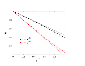
Figure 11: Plot of the bosonic and fermionic maximal velocities $V^{(\rm B)}$ (black) and $V^{(\rm F)}$ (red), characterizing ballistic spreading in a linear confining potential, against $g^{1/2}$. Straight lines: scaling results (4.24) and (4.28) at small $g$.

4.3 Quadratic confining potential

Our second example is the quadratic confining potential

$$W_{m}=gm^{2},$$ (4.32)

where $g$ is again a positive constant. Equation (4.6) reads

$$\omega\chi_{m}=-\gamma(\chi_{m-1}+\chi_{m+1})+gm^{2}\chi_{m}.$$ (4.33)

The Fourier transform $\widehat{\chi}(p)$ therefore obeys

$$g\frac{{\rm d}^{2}\widehat{\chi}}{{\rm d}p^{2}}=-(\omega+2\gamma\cos p)\widehat{\chi}.$$ (4.34)

The latter differential equation is known as the Mathieu equation [46]. The body of knowledge on the latter equation is however of little use for the present purpose. Hereafter we therefore use general techniques which could be applied to any confining potential.

Figure 12 shows the bosonic and fermionic spectra for $g=0.1$. These spectra are qualitatively similar to those shown in figure 10. The existence of two very distinct regions, with strongly dispersive modes within the band and weakly dispersive branches above the band, is indeed a common feature of all confining potentials.

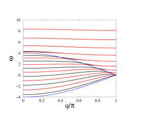
Figure 12: Plot of the bosonic and fermionic spectra for the quadratic confining potential with $g=0.1$, against $q/\pi$. Black: bosonic frequencies $\omega_{k}^{(\rm B)}(q)$. Red: fermionic frequencies $\omega_{k}^{(\rm F)}(q)$. Blue: band boundaries ($\omega=\pm 2\gamma=\pm 4\cos(q/2)$).

Let us first consider the weakly dispersive branches above the band. Right at $\gamma=0$ (this corresponds to $q=\pi$, i.e., to the right end of figure 12), the eigenstates are strictly localized at specific sites: we have $\chi_{m}=\delta_{m,k}$ and $\omega_{k}=W_{k}=gk^{2}$. If $\gamma$ is small and/or $k$ is large, the wavefunction $\chi_{k\pm 1}$ at neighboring sites is proportional to the ratio $\gamma/k$. We thus obtain the more refined estimate

$$\omega_{k}\approx gk^{2}+\frac{2\gamma^{2}}{(4k^{2}-1)g}.$$ (4.35)

High branches are therefore weakly dispersive, as their bandwidth scales as $1/(gk^{2})$. With a linear confining potential, the Wannier-Stark states were not dispersive at all.

In the whole region above the band, the splitting between even (bosonic) and odd (fermionic) frequencies can hardly be observed. This splitting can be estimated as follows. First, it is expected on general grounds to scale as $\chi_{0}^{2}$ (see (4.16)). Furthermore, $\chi_{0}$ is exponentially small whenever $\gamma$ is small and/or $k$ is large. In this regime, (4.33) indeed simplifies to $g(k^{2}-m^{2})\chi_{m}\approx-\gamma\chi_{m+1}$ for $0<m<k$. We thus obtain the estimate

$$|\chi_{0}|\approx\frac{2(\gamma/g)^{k}}{(2k)!}\sim\left(\frac{\rme^{2}\gamma}{4gk^{2}}\right)^{k}.$$ (4.36)

The velocities $V^{(\rm B)}$ and $V^{(\rm F)}$ characterizing the ballistic spreading of an initially localized wavefunction again correspond to the lowest branches of the spectra. In the regime of most interest where $g$ is small, these velocities can be calculated by means of a continuum description. With the notation (4.18), we obtain

$$\gamma\frac{{\rm d}^{2}\chi}{{\rm d}m^{2}}\approx(gm^{2}-\delta)\chi.$$ (4.37)

Setting

$$m=(g/\gamma)^{1/4}x,\qquad\delta=(g\gamma)^{1/2}{\cal E},$$ (4.38)

Equation (4.37) becomes the usual Schrödinger equation for a harmonic oscillator,

$$-\frac{{\rm d}^{2}\chi}{{\rm d}x^{2}}+x^{2}\chi={\cal E}\chi,$$ (4.39)

whose eigenvalues are ${\cal E}_{\nu}=2\nu+1$ ($\nu=0,1,\dots$).

For the bosonic spectrum, the lowest branch corresponds to ${\cal E}_{0}=1$, and so

$$\delta^{(\rm B)}\approx(g\gamma)^{1/2}.$$ (4.40)

Using (4.23), we obtain

$$V^{(\rm B)}\approx 2-C^{(\rm B)}\,g^{2/5},$$ (4.41)

$$C^{(\rm B)}=\frac{5}{2^{14/5}}=0.717936\dots$$ (4.42)

For the fermionic spectrum, the lowest branch corresponds to ${\cal E}_{1}=3$, and so

$$\delta^{(\rm F)}\approx 3(g\gamma)^{1/2},$$ (4.43)

$$V^{(\rm F)}\approx 2-C^{(\rm F)}\,g^{2/5},$$ (4.44)

$$C^{(\rm F)}=\frac{3^{4/5}\,5}{2^{14/5}}=1.728952\dots$$ (4.45)

The ratio of the amplitudes is

$$\frac{C^{(\rm F)}}{C^{(\rm B)}}=3^{4/5}=2.408224\dots$$ (4.46)

Figure 13 shows plots of the maximal velocities $V^{(\rm B)}$ and $V^{(\rm F)}$ against $g^{2/5}$. Here again, the scaling results (4.41) and (4.44) at small $g$ (straight lines) provide a good description of the velocities for moderate values of $g$.

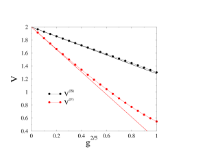
Figure 13: Plot of the bosonic and fermionic maximal velocities $V^{(\rm B)}$ (black) and $V^{(\rm F)}$ (red), characterizing ballistic spreading in a quadratic confining potential, against $g^{2/5}$. Straight lines: scaling results (4.41) and (4.44) at small $g$.

4.4 Confining potential with an arbitrary exponent

We now consider the case of a confining potential of the form

$$W_{m}=g|m|^{\alpha},$$ (4.47)

with an arbitrary exponent $\alpha>0$.

Let us focus on the maximal velocities $V^{(\rm B)}$ and $V^{(\rm F)}$ characterizing the ballistic spreading of a localized initial state. In the most interesting regime when $g$ is small, these velocities can be calculated by means of a continuum description. With the notation (4.18), we obtain

$$\gamma\frac{{\rm d}^{2}\chi}{{\rm d}m^{2}}\approx(g|m|^{\alpha}-\delta)\chi.$$ (4.48)

Setting

$$m=(g/\gamma)^{1/(\alpha+2)}x,\qquad\delta=(g^{2}\gamma^{\alpha})^{1/(\alpha+2)}{\cal E},$$ (4.49)

Equation (4.48) becomes the continuous Schrödinger equation

$$-\frac{{\rm d}^{2}\chi}{{\rm d}x^{2}}+|x|^{\alpha}\chi={\cal E}\chi,$$ (4.50)

whose eigenvalues ${\cal E}_{\nu}$ ($\nu=0,1,\dots$) are not known analytically in general.

For the bosonic spectrum, the lowest branch corresponds to ${\cal E}_{0}$, and so

$$\delta^{(\rm B)}\approx(g^{2}\gamma^{\alpha})^{1/(\alpha+2)}{\cal E}_{0}.$$ (4.51)

Using again (4.23), we obtain

$$V^{(\rm B)}\approx 2-C^{(\rm B)}\,g^{2/(\alpha+3)},$$ (4.52)

$$C^{(\rm B)}=\frac{\alpha+3}{2^{2/(\alpha+3)}}\left(\frac{\alpha{\cal E}_{0}}{(\alpha+2)^{2}}\right)^{(\alpha+2)/(\alpha+3)}.$$ (4.53)

For the fermionic spectrum, the lowest branch corresponds to ${\cal E}_{1}$, and so

$$\delta^{(\rm F)}\approx(g^{2}\gamma^{\alpha})^{1/(\alpha+2)}{\cal E}_{1},$$ (4.54)

$$V^{(\rm F)}\approx 2-C^{(\rm F)}\,g^{2/(\alpha+3)},$$ (4.55)

$$C^{(\rm F)}=\frac{\alpha+3}{2^{2/(\alpha+3)}}\left(\frac{\alpha{\cal E}_{1}}{(\alpha+2)^{2}}\right)^{(\alpha+2)/(\alpha+3)}.$$ (4.56)

The ratio of the amplitudes is

$$\frac{C^{(\rm F)}}{C^{(\rm B)}}=\left(\frac{{\cal E}_{1}}{{\cal E}_{0}}\right)^{(\alpha+2)/(\alpha+3)}.$$ (4.57)

The scaling laws (4.52) and (4.55) generalize (4.24), (4.28), (4.41), (4.44). They can also be put in perspective with (3.16), which holds in the situation where a hard bound $\ell$ is imposed on the distance $|m|$ between both particles. Let us introduce the length $\ell$ as the distance where the potential (4.47) equals unity, i.e.,

$$\ell=g^{-1/\alpha}.$$ (4.58)

In terms of this length parameter, (4.52) and (4.55) take the form

$$V^{(\rm B)}\approx 2-\frac{C^{(\rm B)}}{\ell^{2\alpha/(\alpha+3)}},\qquad V^{(\rm F)}\approx 2-\frac{C^{(\rm F)}}{\ell^{2\alpha/(\alpha+3)}}.$$ (4.59)

These expressions smoothly match their counterparts (3.16) in the $\alpha\to\infty$ limit, where the potential gets infinitely steep. The exponent slowly converges to the limit value 2, while the amplitudes (4.53), (4.56) also converge to the limits (3.17).

The ratio $C^{(\rm F)}/C^{(\rm B)}$ can be viewed as a universal amplitude ratio. This dimensionless quantity depends only on the growth exponent $\alpha$ of the confining potential (see (4.57)), increasing monotonically from 1 in the singular $\alpha\to 0$ limit to 4 in the $\alpha\to\infty$ (i.e., hard-bound) limit. Its values for $\alpha=1$ and $\alpha=2$ have been given in (4.31) and (4.46). Figure 14 shows a plot of this ratio against $\alpha/(\alpha+1)$.

Finally, the amplitude ratio $C^{(\rm F)}/C^{(\rm B)}$ is always larger than unity. More generally, bosonic bound states always have a larger maximal spreading velocity than fermionic bound states in the same confining potential. We shall come back to this very common property in section 5.

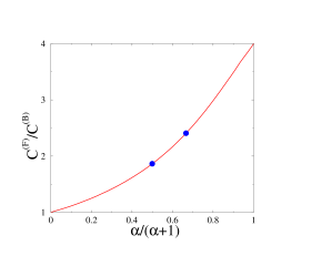
Figure 14: Plot of the universal amplitude ratio $C^{(\rm F)}/C^{(\rm B)}$ against $\alpha/(\alpha+1)$, where $\alpha$ is the growth exponent of the confining potential. Symbols: results (4.31) and (4.46) for $\alpha=1$ and $\alpha=2$. Curve: data points obtained by means of a numerical calculation of the eigenvalues ${\cal E}_{0}$ and ${\cal E}_{1}$ of (4.50).

5 Discussion

In this work we have investigated the continuous-time quantum walk performed along a one-dimensional lattice by bound states of two interacting particles. The main focus has been on the profile of the wavefunctions describing these bound states in the center-of-mass coordinate, and especially on the velocity characterizing their ballistic spreading and on the structure of the whole profile, which generically exhibits many internal fronts.

We have first revisited the problem of a single quantum walker in a self-contained pedagogical fashion. For the simple quantum walk where the particle hops to nearest neighbors only, we have concentrated onto the dependence of the distribution of the particle position on the initial state. This distribution profile has generically two ballistic fronts. Either one or even both fronts may be absent for carefully chosen special initial states, as this was already the case for some examples of discrete-time walks [20, 32, 33, 37]. For the generalized quantum walk, where the particle hops to first and second neighbors with respective amplitudes 1 and $g$, we have emphasized the possible occurrence of two internal fronts in the distribution profile, propagating at velocities $\pm V_{-}$, besides the two usual external ones, propagating at velocities $\pm V_{+}$, which mark the endpoints of the allowed region beyond which the wavefunction falls off exponentially. The non-trivial dependence of the velocities $V_{\pm}$ on the amplitude $g$ is in contrast with the equally spaced internal peaks arising for the discrete-time quantum walks considered in earlier works [31, 34].

The quantum walk of bound states of two bosonic or fermionic particles has then been investigated in two situations: either by imposing a hard bound $\ell$ on the distance between both particles, or by generating the bound states by a smooth confining potential growing as a power of the distance. In both situations, we have focused on the structure of the distribution of the center-of-mass coordinate. We have investigated in detail the maximal velocities $V^{(\rm B)}$ and $V^{(\rm F)}$ characterizing the ballistic spreading of bosonic and fermionic bound states, as well as the many internal fronts of their distribution profiles. In the case of a hard distance bound (section 3), the maximal velocities have the simple expressions (3.15). The distribution profile generically exhibits $\ell-1$ (resp. $\ell-2$) internal fronts in the bosonic (resp. fermionic) case, besides the two extremal ballistic fronts. In the situation of a smooth confining potential (section 4), we have investigated in detail the cases of a linear and of a quadratic (i.e., discrete harmonic) potential. For all potentials of the form $W_{m}=g|m|^{\alpha}$, growing as a power of the distance between both particles, the maximal velocities exhibit scaling laws of the form (4.52), (4.55) in the regime of a weak potential ($g\ll 1$). The associated amplitude ratio $C^{(\rm F)}/C^{(\rm B)}$ is universal, in the sense that it depends only on the growth exponent $\alpha$ of the confining potential. This ratio is larger than unity, in accord with the more general property that bosonic bound states have a larger maximal spreading velocity than their fermionic counterparts in the same binding potential.

Let us now compare our findings with those of two recent papers [21, 25] which are also devoted to the quantum walk of bound states. The latter works deal with full two-body Hamiltonians, along the lines of earlier investigations of the Anderson localization of two interacting particles [12, 13, 14]. In such models bound states therefore coexist with a full two-particle continuum. The situations studied in the present work (hard distance bound or confining potential) only possess bound states, so that the investigation of the latter is made easier. As internal ballistic fronts are not discussed in [21, 25], we shall henceforth concentrate on the maximal spreading velocity $V$. Reference [21] deals with the antisymmetric (i.e., fermionic) sector of a discrete-time model, with a local interaction described by the action of a special coin operator whenever both particles sit at the same site. The associated coupling constant $g$ is an angle. The analysis of the bound-state spectrum allows one to derive the maximal velocity $V$. This quantity (whose expression is not explicitly given in [21]) decreases continuously from $1/\sqrt{2}$ to $1/3$ as $g$ is increased from 0 to its maximal value of $\pi$. Reference [25] describes the continuous-time dynamics of two identical particles (either bosons or fermions) generated by a Hubbard-like Hamiltonian with nearest-neighbor interactions. The maximal velocities are derived by means of a perturbative approach in the regime of very strongly attractive interactions. Both spreading velocities are found to fall off to zero as the inverse of the interaction strength, and to obey the simple relation $V^{(\rm B)}=3V^{(\rm F)}$.

Even though very different models and regimes have been considered, all the findings recalled above are consistent with the following universal characteristics of the ballistic spreading of two-body bound states. For a given interaction strength, bosonic bound states always have a larger velocity of spreading than their fermionic counterparts. When the interaction strength is increased, the spreading velocity decreases continuously from its free one-body value down to zero or to a much smaller limiting value.

A natural extension of the present work consists in considering the quantum walk performed by bound states of more than two identical particles. A classical analogue consists of multi-pedal molecular devices whose legs perform random walks, known as molecular spiders [47]. Their behavior has been investigated theoretically, both on a one-dimensional [48] and a two-dimensional [49] substrate. The quantum version of the problem yields a special kind of $N$-fermion bound state, which can be analyzed by techniques from integrable systems. This will be the subject of future work [50].

Appendix A Stationary properties of a quantum system

In this appendix we investigate the stationary properties of a finite quantum system from a very general standpoint. Consider a quantum system whose Hilbert space has finite dimension $N$, working in a preferred basis $|a\rangle$ $(a=1,\dots,N)$. In this basis, the Hamiltonian is given by an $N\times N$ Hermitian matrix $H$. Assume that the energy eigenvalues $E_{n}$ $(n=1,\dots,N)$ are non-degenerate. Let $|n\rangle$ be normalized eigenvectors, so that $H|n\rangle=E_{n}|n\rangle$. Assuming the system is initially in state $|a\rangle$, we have

$$|\psi(t)\rangle=\sum_{n}\rme^{-{\rm i}E_{n}t}|n\rangle\langle n|a\rangle.$$ (1.1)

The probability of observing the system is state $|b\rangle$ at time $t$ reads therefore in full generality

$$P_{ab}(t)=|\langle b|\psi(t)\rangle|^{2}=\sum_{m,n}\rme^{{\rm i}(E_{n}-E_{m})t}\langle b|m\rangle\langle m|a\rangle\langle a|n\rangle\langle n|b\rangle.$$ (1.2)

We are interested in the stationary transition probabilities

$$Q_{ab}=\lim_{t\to\infty}\frac{1}{t}\int_{0}^{t}P_{ab}(t^{\prime})\,{\rm d}t^{\prime}.$$ (1.3)

In the absence of spectral degeneracies, only diagonal terms $(m=n)$ in the double sum in (1.2) contribute. We thus obtain

$$Q_{ab}=\sum_{n}|\langle a|n\rangle|^{2}|\langle b|n\rangle|^{2}.$$ (1.4)

The matrix $Q$ is real symmetric and positive definite. It reads indeed

$$Q=RR^{T},$$ (1.5)

with

$$R_{an}=|\langle a|n\rangle|^{2}.$$ (1.6)

The matrix $Q$ is non-trivial in general. This is a manifestation of the well-known fact that a finite isolated quantum system does not equilibrate, in the sense that its stationary properties remember its initial state forever.

We now turn to the explicit example of a confined quantum walker, i.e., a tight-binding particle on a finite segment of $N$ sites labelled $a=1,\dots,N$. The preferred basis is chosen to be local in space. The Hamiltonian reads

$$\langle a|H|\psi\rangle=\psi_{a+1}+\psi_{a-1},$$ (1.7)

where $\langle a|\psi\rangle=\psi_{a}$ and with Dirichlet boundary conditions $\psi_{0}=\psi_{N+1}=0$. We have

$$E_{n}=2\cos\frac{n\pi}{N+1},\qquad\langle a|n\rangle=\sqrt{\frac{2}{N+1}}\sin\frac{an\pi}{N+1},$$ (1.8)

($n=1,\dots,N$), and so

$$Q_{ab}=\left(\frac{2}{N+1}\right)^{2}\sum_{n}\sin^{2}\frac{an\pi}{N+1}\sin^{2}\frac{bn\pi}{N+1}.$$ (1.9)

This sum can be worked out explicitly. We thus obtain

$$Q_{ab}=\frac{1}{N+1}\left(1+\frac{1}{2}\delta_{a,b}+\frac{1}{2}\delta_{a+b,N+1}\right).$$ (1.10)

With respect to its uniform background value $1/(N+1)$, the stationary probability $Q_{ab}$ is thus enhanced by a factor 3/2 both at the starting point ($b=a$) and at the symmetric position ($b=N+1-a$). In the particular situation where the starting point is the middle of an odd segment ($N$ odd and $a=(N+1)/2$), the enhancement factor of the return probability reaches 2.

The stationary mean value of the position $X$ of a walker launched at site $a$, i.e.,

$$\langle X\rangle=\sum_{b}bQ_{ab}=\frac{N+1}{2},$$ (1.11)

is dictated by symmetry, and therefore independent of the initial state. The corresponding variance,

$$\langle X^{2}\rangle-\langle X\rangle^{2} = \sum_{b}b^{2}Q_{ab}-\biggl{(}\sum_{b}bQ_{ab}\biggr{)}^{2}$$ (1.12)

$$= \frac{N(N-1)}{12}+\frac{(N+1-2a)^{2}}{4(N+1)},$$

however shows a dependence on the initial position $a$ of the walker.

For $N=4$ we obtain

$$Q=\frac{1}{10}\pmatrix{3&2&2&3\cr 2&3&3&2\cr 2&3&3&2\cr 3&2&2&3}.$$ (1.13)

The first row, i.e.,

$$Q_{11}=Q_{14}=\frac{3}{10},\qquad Q_{12}=Q_{13}=\frac{1}{5},$$ (1.14)

agrees with the result (3.34) of a full dynamical analysis of the two-fermion bound state with $N=\ell=4$.

References

References

- [1] Kempe J 2003 Contemp. Phys. 44 307–327
- [2] Ambainis A 2003 Int. J. Quant. Inf. 1 507–518
- [3] Venegas-Andraca S E 2012 Quant. Inf. Processing 11 1015–1106
- [4] Aharonov Y, Davidovich L and Zagury N 1993 Phys. Rev. A 48 1687–1690
- [5] Konno N 2002 Quant. Inf. Processing 1 345–354
- [6] Konno N 2005 J. Math. Soc. Japan 57 1179–1195
- [7] Mackay T D, Bartlett S D, Stephenson L T and Sanders B C 2002 J. Phys. A 35 2745–2753
- [8] Farhi E and Gutmann S 1998 Phys. Rev. A 58 915–928
- [9] de Toro Arias S and Luck J M 1998 J. Phys. A 31 7699–7717
- [10] ben Avraham D, Bollt E M and Tamon C 2004 Quant. Inf. Processing 3 295–308
- [11] Strauch F W 2006 Phys. Rev. A 74 030301
- [12] Shepelyansky D L 1994 Phys. Rev. Lett. 73 2607–2610
- [13] Imry Y 1995 Europhys. Lett. 30 405–408
- [14] Krimer D O and Flach S 2015 Phys. Rev. B 91 100201(R)
- [15] Omar Y, Paunkovic N, Sheridan L and Bose S 2006 Phys. Rev. A 74 042304
- [16] Gamble J K, Friesen M, Zhou D, Joynt R and Coppersmith S N 2010 Phys. Rev. A 81 052313
- [17] Berry S D and Wang J B 2011 Phys. Rev. A 83 042317
- [18] Mayer K, Tichy M C, Mintert F, Konrad T and Buchleitner A 2011 Phys. Rev. A 83 062307
- [19] Rohde P P, Schreiber A, Stefanak M, Jex I and Silberhorn C 2011 New J. Phys. 13 013001
- [20] Stefanak M, Barnett S M, Kollar B, Kiss T and Jex I 2011 New J. Phys. 13 033029
- [21] Ahlbrecht A, Alberti A, Meschede D, Scholz V B, Werner A H and Werner R F 2012 New J. Phys. 14 073050
- [22] Lahini Y, Verbin M, Huber S D, Bromberg Y, Pugatch R and Silberberg Y 2012 Phys. Rev. A 86 011603(R)
- [23] Benedetti C, Buscemi F and Bordone P 2012 Phys. Rev. A 85 042314
- [24] Chandrashekar C M and Busch T 2012 Quant. Inf. Processing 11 1287–1299
- [25] Qin X, Ke Y, Guan X, Li Z, Andrei N and Lee C 2014 Phys. Rev. A 90 062301
- [26] Fukuhara T, Schauss P, Endres M, Hild S, Cheneau M, Bloch I and Gross C 2013 Nature 502 76–79
- [27] Peruzzo A, Lobino M, Matthews J C F, Matsuda N, Politi A, Poulios K, Zhou X Q, Lahini Y, Ismail N, Wörhoff K, Bromberg Y, Silberberg Y, Thompson M G and OBrien J L 2010 Science 329 1500–1503
- [28] Sansoni L, Sciarrino F, Vallone G, Mataloni P, Crespi A, Ramponi R and Osellame R 2012 Phys. Rev. Lett. 108 010502
- [29] Crespi A, Osellame R, Ramponi R, Giovannetti V, Fazio R, Sansoni L, Nicola F D, Sciarrino F and Mataloni P 2013 Nature Photonics 7 322–328
- [30] Preiss P M, Ma R, Tai M E, Lukin A, Rispoli M, Zupancic P, Lahini Y, Islam R and Greiner M 2015 Science 347 1229–1233
- [31] Brun T A, Carteret H A and Ambainis A 2003 Phys. Rev. A 67 052317
- [32] Tregenna B, Flanagan W, Maile R and Kendon V 2003 New J. Phys. 5 83
- [33] Inui N, Konno N and Segawa E 2005 Phys. Rev. E 72 056112
- [34] Miyazaki T, Katori M and Konno N 2007 Phys. Rev. A 76 012332
- [35] Falkner S and Boettcher S 2014 Phys. Rev. A 90 012307
- [36] Machida T 2015 Quant. Inf. and Comput. 15 406–418
- [37] Stefanak M, Bezdekova I and Jex I 2014 Phys. Rev. A 90 012342
- [38] Geim A K and Novoselov K S 2007 Nature Materials 6 183–191
- [39] Castro-Neto A H, Guinea F, Peres N M R, Novoselov K S and Geim A K 2009 Rev. Mod. Phys. 81 109–162
- [40] Watson G N 1958 A Treatise on the Theory of Bessel Functions (Cambridge: Cambridge University Press)
- [41] Erdélyi A 1953 Higher Transcendental Functions (The Bateman Manuscript Project) (New York: McGraw-Hill)
- [42] Privitera A and Capone M 2012 Phys. Rev. A 85 013640
- [43] Vilenkin N A 1988 Special Functions and the Theory of Group Representations (Providence, RI: American Mathematical Society)
- [44] Wannier G H 1959 Elements of Solid State Theory (Cambridge: Cambridge University Press)
- [45] Wannier G H 1962 Rev. Mod. Phys. 34 645–655
- [46] Abramowitz M and Stegun I A 1974 Handbook of Mathematical Functions (New York: Dover)
- [47] Pei R, Taylor S K, Stefanovic D, Rudchenko S, Mitchell T E and Stojanovic M N 2006 J. Amer. Chem. Soc. 128 12693–12699
- [48] Antal T, Krapivsky P L and Mallick K 2007 J. Stat. Mech. 2007 P08027
- [49] Antal T and Krapivsky P L 2012 Phys. Rev. E 85 061927
- [50] Krapivsky P L, Luck J M and Mallick K (in preparation)