The southern molecular environment of SNR G18.8+0.3

Abstract

Aims. In a previous paper we have investigated the molecular environment towards the eastern border of the SNR G18.8+0.3. Continuing with the study of the surroundings of this SNR, in this work we focus on its southern border, which in the radio continuum emission shows a very peculiar morphology with a corrugated corner and a very flattened southern flank.

Methods. We observed two regions towards the south of SNR G18.8+0.3 using the Atacama Submillimeter Telescope Experiment (ASTE) in the ¹²CO J=3–2. One of these regions was also surveyed in ¹³CO and C¹⁸O J=3–2. The angular and spectral resolution of these observations were 22^′′, and 0.11 km s^-1. We compared the CO emission to 20 cm radio continuum maps obtain as part of the Multi-Array Galactic Plane Imaging Survey (MAGPIS) and 870 $\mu$m dust emission extracted from the APEX Telescope Large Area Survey of the Galaxy.

Results. We discovered a molecular feature with a good morphological correspondence with the SNR’s southernmost corner. In particular, there are indentations in the radio continuum map that are complemented by protrusions in the molecular CO image, strongly suggesting that the SNR shock is interacting with a molecular cloud. Towards this region we found that the ¹²CO peak is not correlated with the observed ¹³CO peaks, which are likely related to a nearby Hii region. Regarding the most flattened border of SNR G18.8+0.3, where an interaction of the SNR with dense material was previously suggested, our ¹²CO J=3–2 map show no obvious indication that this is occurring.

1 Introduction

The investigation of the surroundings of supernova remnants (SNRs) can provide useful information for a wide range of research fields, as the physical and chemical changes induced by the passage of a shock wave, dust production and destruction, the possibility of triggering stellar formation, production of high-energy gamma rays, etc. Multiwavelength studies are required to explore these effects.

The SNR G18.8+0.3, with a peculiar shape with flattened borders along the east and south, has been suggested to be interacting with dense molecular gas towards such directions (Dubner et al. 1999, 2004; Tian et al. 2007). Paron et al. (2012), hereafter Paper I, investigated the molecular gas towards the eastern border of the SNR G18.8+0.3. They found a dense molecular clump, close to the shock front of the SNR but not in contact with it, containing a complex of Hii regions and massive young stellar objects (YSOs) deeply embedded. This region is indicated in Fig. 1 as ‘Eastern Clump’. Figure 1 shows the SNR G18.8+0.3 in radio continuum at 20 cm as extracted from the MAGPIS (Helfand et al. 2006) (in blue) and its surroundings as seen at the 870 $\mu$m emission extracted from the ATLASGAL (Beuther et al. 2012) (in green). Southwards of the SNR, where the molecular cloud appears to be in contact with SNR shock front (see Figure 1 in Paper I), there are a few Hii regions and submillimeter dust compact sources, making this region an interesting target to study the interplay between the SNR shock front, surrounding molecular gas, and Hii regions.

Using molecular lines we investigate two regions towards the south of SNR G18.8+0.3; Reg.1 and the subregion Reg.1b, were selected to investigate the possible causes for the peculiar morphology of the SNR southernmost ‘corner’, and the molecular gas towards the Hii region G018.630+0.309 (Anderson et al. 2011) and the ATLASGAL source 018.626+00.297 (Urquhart et al. 2014), while Reg.2 was chosen to investigate the molecular environment towards the most flattened border of the SNR where originally it was suggested an interaction with a dense cloud (Dubner et al. 1999). As in Paper I, here we assume a distance of $14\pm 1$ kpc for SNR G18.8+0.3. Concerning to the Hii region G018.630+0.309, Anderson et al. (2012) could not resolve the distance ambiguity between 1.5 and 14.7 kpc.

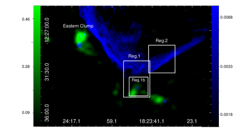
Figure 1: Two-color image of the SNR G18.8+0.3 and its surroundings. The radio continuum emission at 20 cm (from MAGPIS) is displayed in blue (right color bar), and the ATLASGAL emission at 870 $\mu$m in green (left color bar). Both color ranges are in Jy beam^-1. The surveyed regions in the molecular lines using ASTE are indicated.

2 Observations

The observations of the molecular lines were carried out between September 7 and 13, 2013 with the 10 m Atacama Submillimeter Telescope Experiment (ASTE; Ezawa et al. 2004). We used the CATS345 receiver, which is a two-single band SIS receiver remotely tunable in the LO frequency range of 324-372 GHz. The surveyed regions are shown in Fig. 1 and summarized in Table 1. The observations were performed in position switching mode and the mapping grid spacing was 20^′′ in all cases. The ¹²CO J=3–2 line (345.796 GHz) was observed towards Regs. 1, 2. In Reg.1b we also observed C¹⁸O J=3–2 (329.330 GHz), and ¹³CO J=3–2 (330.587 GHz). The integration time was 20 sec for the ¹²CO and 50 sec for the other molecular lines in each pointing.

Table 1: Surveyed regions using ASTE.

Region	Center (R.A., dec.)	Size
Reg.1	18:23:48.0, $-$12:32:14.5	3′$\times$4′
Reg.1b	18:23:47.1, $-$12:33:12.1	2′$\times$2′
Reg.2	18:23:38.0, $-$12:30:04.6	3′$\times$3′

We used the XF digital spectrometer with bandwidth and spectral resolution set to 128 MHz and 125 kHz, respectively. The velocity resolution was 0.11 km s^-1, the half-power beamwidth (HPBW) 22^′′, and the main beam efficiency was $\eta_{\rm mb}\sim 0.65$. The spectra were Hanning smoothed to improve the signal-to-noise ratio and only linear or some second order polynomia were used for baseline fitting. The data were reduced with NEWSTAR and the spectra processed using the XSpec software package.

3 Results and discussion

3.1 Regions 1 and 1b

In Reg.1, ¹²CO J=3–2 emission is detected at velocities between 5 and 30 km s^-1, very much like what was observed in the eastern region (Paper I). The emission integrated over the mentioned velocity range is displayed as contours over a two-color image showing the 20 cm and 870 $\mu$m continuum images in Fig. 2. Importantly, the boundaries of the radio continuum emission from the SNR and the ¹²CO emission from the molecular cloud show a number of common features, strongly suggesting that the shock front is interacting with the cloud. In particular, the most noticeable indentations in the border of the SNR are complemented by protrusions in the molecular cloud. In addition, towards the south the contour at 56 K km s^-1 of the ¹²CO emission has a peculiar curvature apparently in coincidence with the Hii region G018.630+0.309, suggesting that this object is also associated with the molecular structure.

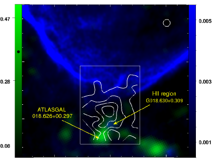
Figure 2: Two-color image towards Reg.1 with the radio continuum emission at 20 cm (from MAGPIS) displayed in blue (right color bar), and the ATLASGAL emission at 870 $\mu$m in green (left color bar). Both color ranges are in Jy beam^-1. The ¹²CO J=3–2 emission integrated between 5 and 30 km s^-1 is presented in contours, with levels of 32, 42, 56, and 68 K km s^-1. The beam of the molecular observations is shown at the top right corner. The positions of the Hii region G018.630+0.309 and the compact dust source ATLASGAL 018.626+00.297 are indicated.

Figure 3 displays the ¹³CO J=3–2 emission integrated between 15 and 26 km s^-1 towards Reg.1b in white contours. For context, the 56, and 68 K km s^-1 contours of the ¹²CO emission shown in Fig. 2 are also shown in Fig. 3 (yellow dashed contours). The ¹³CO emission reveals a molecular feature, composed by two clumps, that partially surrounds the Hii region G018.630+0.309. One of these clumps, the southernmost, exactly overlaps the source ATLASGAL 018.626+00.297. Curiously the most intense emission of the ¹²CO is not correlated with the ¹³CO peaks. Concerning the C¹⁸O J=3–2 line, we only detect emission (a single spectrum) over the maximum of the ATLASGAL source, implying that this is the region with highest density.

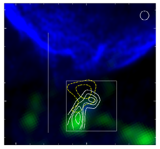
Figure 3: Two-color image towards Reg.1b with the radio continuum emission at 20 cm (from MAGPIS) displayed in blue, and the ATLASGAL emission at 870 $\mu$m in green. The color ranges are the same as in Fig. 2. For context, the box of Reg.1 and the 56, and 68 K km s^-1 contours (in dashed yellow line) of the ¹²CO emission presented in Fig. 2 are also shown. Contours of the ¹³CO J=3–2 emission integrated between 15 and 26 km s^-1 are shown in white, with levels of 12.0, 15.0, 16.5, and 20.0 K km s^-1. The beam of the molecular observations is shown at the top right corner.

In order to discuss the molecular gas in Reg.1 and Reg.1b we denote the structure delimited by the 56 K km s^-1 contour (the dashed yellow contour in Fig. 3) as the “¹²CO-clump”, the feature delimited by a circle of 25^′′ in radius centered at the northern maximum in the ¹³CO emission is designated as the “¹³CO-clumpN”, and the southern ¹³CO clump delimited by the 16.5 K km s^-1 contour as the “¹³CO-clumpS” (see Fig 3). We estimated the mass of these features applying a variety of methods, namely: by assuming local thermodynamic equilibrium (LTE), from the CO luminosity (in the case of the ¹²CO-clump), from the thermal dust emission at 870 $\mu$m (in the case of the ¹³CO-clumpS), and based on the virial theorem. To obtain the LTE mass, we follow the procedures described in Paper I to estimate the column densities of N(¹²CO) and N(¹³CO). Table 2 presents the derived and used parameters to perform that. The column density values represent the total column density as obtained from summation over all beam positions belonging to each molecular structure described above. To obtain the mass from the CO luminosity we use (e.g. Bertsch et al. 1993): ${\rm N(H_{2})}=2\times 10^{20}\leavevmode\nobreak\ {\rm W(^{12}CO)}$ to estimate N(H₂), where W(¹²CO) is the velocity integrated ¹²CO emission along the whole ¹²CO-clump structure. Finally, once obtained the total N(H₂), either from the LTE approximation or from the CO luminosity, the mass is derived using ${\rm M}=\mu\leavevmode\nobreak\ m_{{\rm H}}\leavevmode\nobreak\ d^{2}\leavevmode\nobreak\ \Omega\leavevmode\nobreak\ {\rm N(H_{2}})$, where $\Omega$ is the solid angle subtended by the beam size, $m_{\rm H}$ is the hydrogen mass, $\mu$, the mean molecular weight, assumed to be 2.8 by taking into account a relative helium abundance of 25 %, and $d$ is the distance.

Assuming that the ¹³CO-clumpS is related to the ATLASGAL source 018.626+00.297, we estimate its mass from the thermal dust emission at 870 $\mu$m following the procedure presented in Csengeri et al. (2014). We use an integrated flux of S${}_{\rm int}=3.31$ Jy (Urquhart et al. 2014), and assume a typical dust temperature of T${}_{\rm d}=15$ K.

Finally, the virial mass of the three molecular structures is derived from the relation:

$${\rm M_{vir}}=\frac{5\leavevmode\nobreak\ {\rm R_{clump}}(\Delta{\rm v})^{2}}{8\leavevmode\nobreak\ {\rm G}\leavevmode\nobreak\ {\rm ln(2)}}$$ (1)

where G, R_clump and $\Delta$v are the gravitational constant, the clump radius (assuming a spherical geometry), and the line width, respectively. Following Saito et al. (2007) we define the clump radius as the deconvolved radius calculated from ${\rm R_{clump}}=\sqrt{\frac{S-{\rm beam\leavevmode\nobreak\ area}}{\pi}}$, where $S$ is the area inside the clump. The velocity width $\Delta$v was derived through a Gaussian fitting to the averaged spectrum obtained for the molecular features. The deconvolved radius (${\rm R_{clump}}$) are 2.95, 1.52, and 1.05 pc, and the $\Delta$v $=$ 7.05, 3.80, and 5.10 km s^-1 for the ¹²CO-clump, ¹³CO-clumpN, and ¹³CO-clumpS, respectively. All mass results are presented in Table 3.

Table 2: Used and derived parameters for the LTE mass.

Parameter	12CO-clump	13CO-clumpN	13CO-clumpS
Tex (K)	16.6	12.5	11.0
$\tau^{12}$	15	–	–
$\tau^{13}$	–	1.3	3.5
N(12CO) (cm-2)	7.1 $\times 10^{18}$	–	–
N(13CO) (cm-2)	–	1.5 $\times 10^{17}$	3.5 $\times 10^{17}$
N(H2) (cm-2)	7.1 $\times 10^{22}$	7.5 $\times 10^{22}$	1.7 $\times 10^{23}$

Table 3: Mass values.

Clump	MLTE	M${}_{\rm CO\leavevmode\nobreak\ lum.}$	Mdust	Mvir
	(M⊙)	(M⊙)	(M⊙)	(M⊙)
12CO-clump	$2.7\times 10^{3}$	$6.0\times 10^{3}$	–	$3.1\times 10^{4}$
13CO-clumpN	$3.0\times 10^{3}$	–	–	$4.5\times 10^{3}$
13CO-clumpS	$7.0\times 10^{3}$	–	$5.5\times 10^{3}$	$5.7\times 10^{3}$

The only case in which the virial mass differs considerably from the mass obtained by other methods is for the ¹²CO-clump. For this feature, the virial mass is almost an order of magnitude larger than the LTE and CO luminosity based-estimates of the mass. This suggests that this feature is not gravitationally bound.

We assume as a working hypothesis that the ¹²CO-clump is a small molecular feature supported by external pressure. The external pressure ($P_{ext}$) required for the ¹²CO-clump to remain bound, can be roughly evaluated from the following expression of the virial theorem (e.g. Kawamura et al. 1998):

$${2U+\Omega-4\pi{\rm R_{clump}}^{3}P_{ext}=0}$$ (2)

where

$$U=3/2\leavevmode\nobreak\ {\rm M}\leavevmode\nobreak\ \frac{\Delta{\rm v}^{2}}{8{\rm ln}(2)},\leavevmode\nobreak\ \leavevmode\nobreak\ {\rm and}\leavevmode\nobreak\ \leavevmode\nobreak\ \Omega=-\frac{3{\rm G}{\rm M}^{2}}{5{\rm R_{clump}}}$$ (3)

Using a mean value between M_LTE and M${}_{\rm CO\leavevmode\nobreak\ lum.}$ for the mass, we obtain that it is required a $P_{ext}/k_{B}\sim 1.4\times 10^{6}$ cm^-3 K, with $k_{B}$ the Boltzmann constant, to keep the ¹²CO-clump bound. This value is at least one order of magnitude larger than the external pressures calculated in Kawamura et al. (1998) for a sample of clouds, where it is considered that the pressure is produced by the surrounding diffuse ambient gas. Thus, if this clump is supported by external pressure it is required a pressure source, which in the present context it is likely to be the SNR shocks running into the outer layers of the molecular gas. The derived $P_{ext}/k_{B}$ is very similar to the pressure obtained towards a region associated with the face-on shock in the Vela SNR using FUSE observations (Sankrit et al. 2001), providing further support to our hypothesis that a SNR shock front contributes to maintain bound the observed ¹²CO-clump.

Finally we perform a SED analysis to the IR counterpart of Hii region G018.630+0.30, the WISE source J182348.08-123316.1 (Cutri & et al. 2013; Wright et al. 2010). The fitting of the SED was done using the tool developed by Robitaille et al. (2007) considering the fluxes at the WISE 3.4, 4.6, 12, and 22 $\mu$m bands, an $A_{v}$ between 14 and 50 mag. (see Paper I) and a distance range of 13–15 kpc. The SED results show that the source is indeed a young massive star (age $\sim$10⁵ yrs and mass $\sim 12$ M_⊙), suggesting that its formation should be approximately coeval with the SN explosion. If the SED is performed using the near distance (a range 1–3 kpc), we find that the source should have a lower mass (about 3 M_⊙), which would be unable to ionize the gas and generate an Hii region. This is an indirect confirmation that the Hii region are located at the farther distance, suggesting that it should be embedded in the molecular cloud southwards the SNR.

3.2 Region 2

The ¹²CO emission from this region is significantly weaker than that detected towards Reg.1. By integrating the ¹²CO J=3–2 emission between 15 and 30 km s^-1 (see Fig. 4-up), the whole velocity range where there is emission, we do not find any conspicuous morphological correspondence between the molecular gas and the most flattened border of the SNR which might suggests some kind of interaction. To appreciate in more detail the behavior of the molecular gas in this region, we present in Fig. 4-bottom the ¹²CO emission in a series of channel maps integrated in steps of 2 km s^-1. It can be seen that the molecular gas has a very clumpy distribution not only in the plane of the sky but also along the line of sight. The ¹²CO emission shown in the three first panels in Fig. 4-bottom may correspond to gas located in front (along the line of sight) of the SNR G18.9+0.3, while the emission displayed in the remaining panels would suggest a correspondence between the SNR and the molecular gas (see mainly the small clump towards the west at panel 24.5 and 26.5km s^-1). We note that the molecular emission towards the bottom left corner of the surveyed region, mainly at 22.5 km s^-1, should belong to the upper right border of the structure analysed in Reg.1. Thus, even though the gas distribution in the last panels of Fig. 4-bottom may suggest a correspondence between the SNR and the molecular gas, these results allow us to conclude that the unusual flattened border of SNR G18.8+0.3 must have some physical origin other than interaction with dense environmental gas.

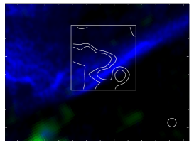
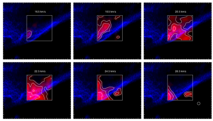
Figure 4: Left: ¹²CO J=3–2 emission integrated between 15 and 30 km s^-1, with levels of 14, 18, and 28 K km s^-1 (white contours) towards Reg.2. The color ranges are the same as in Fig. 2. Right: channel maps of the ¹²CO J=3–2 emission (red with white contours) integrated in steps of 2 km s^-1. The contours levels are 2.5, 4.0, and 6.0 K km s^-1.

4 Summary and concluding remarks

We report the analysis of the molecular gas towards the southern environment of the SNR G18.8+0.3 using ASTE observations. We have surveyed two regions, one towards the SNR southernmost ‘corner’ which in addition harbors the Hii region G018.630+0.309, and a second one towards the most flattened border of the SNR. The main results can be summarized as follows:

(a) In the first region, named Reg.1/Reg.1b, we discovered a molecular feature with a good morphological correspondence with the SNR southernmost corner, where the indentations in the morphology of the SNR radio continuum emission are complemented by protrusions in the molecular cloud, strongly suggesting a SNR-molecular cloud interaction. Additionally, analysing this molecular cloud with the ¹³CO J=3–2 line we found a molecular feature composed by two clumps, not correlated with the ¹²CO peak, that partially surrounds the Hii region G018.630+0.309 and correlates with the thermal dust emission at 870 $\mu$m. We found that the virial mass of the ¹²CO-clump considerably differ from the mass value obtained through other methods, suggesting that it is not gravitationally bound. Finally, from a SED fitting to the IR counterpart of the Hii region, we confirm that it is located at the far distance, suggesting that it should be embedded in the molecular cloud southwards the SNR.

(b) The second region, named Reg.2, covers a portion of the most flattened border of SNR G18.8+0.3, where originally it was suggested an interaction with a dense cloud (Dubner et al. 1999). Strikingly, our ¹²CO J=3–2 observations show a clumpy molecular structure without any morphological correspondence with the flat border of the SNR that could suggest a causal relationship. The better angular resolution attained in these new data served to reveal that the flat southern border of the SNR must originate in a different process other than the compression of a dense molecular cloud.

References

- Anderson et al. (2011) Anderson, L. D., Bania, T. M., Balser, D. S., & Rood, R. T. 2011, ApJS, 194, 32
- Anderson et al. (2012) Anderson, L. D., Bania, T. M., Balser, D. S., & Rood, R. T. 2012, ApJ, 754, 62
- Bertsch et al. (1993) Bertsch, D. L., Dame, T. M., Fichtel, C. E., et al. 1993, ApJ, 416, 587
- Beuther et al. (2012) Beuther, H., Tackenberg, J., Linz, H., et al. 2012, ApJ, 747, 43
- Csengeri et al. (2014) Csengeri, T., Urquhart, J. S., Schuller, F., et al. 2014, A&A, 565, A75
- Cutri & et al. (2013) Cutri, R. M. & et al. 2013, VizieR Online Data Catalog: AllWISE Data Release, 2328, 0
- Dubner et al. (1999) Dubner, G., Giacani, E., Reynoso, E., et al. 1999, AJ, 118, 930
- Dubner et al. (2004) Dubner, G., Giacani, E., Reynoso, E., & Parón, S. 2004, A&A, 426, 201
- Ezawa et al. (2004) Ezawa, H., Kawabe, R., Kohno, K., & Yamamoto, S. 2004, in Society of Photo-Optical Instrumentation Engineers (SPIE) Conference Series, ed. J. M. Oschmann, Jr., Vol. 5489, 763–772
- Helfand et al. (2006) Helfand, D. J., Becker, R. H., White, R. L., Fallon, A., & Tuttle, S. 2006, AJ, 131, 2525
- Kawamura et al. (1998) Kawamura, A., Onishi, T., Yonekura, Y., et al. 1998, ApJS, 117, 387
- Paron et al. (2012) Paron, S., Ortega, M. E., Petriella, A., et al. 2012, A&A, 547, A60
- Robitaille et al. (2007) Robitaille, T. P., Whitney, B. A., Indebetouw, R., & Wood, K. 2007, ApJS, 169, 328
- Saito et al. (2007) Saito, H., Saito, M., Sunada, K., & Yonekura, Y. 2007, ApJ, 659, 459
- Sankrit et al. (2001) Sankrit, R., Shelton, R. L., Blair, W. P., Sembach, K. R., & Jenkins, E. B. 2001, ApJ, 549, 416
- Simon et al. (2001) Simon, R., Jackson, J. M., Clemens, D. P., Bania, T. M., & Heyer, M. H. 2001, ApJ, 551, 747
- Tian et al. (2007) Tian, W. W., Leahy, D. A., & Wang, Q. D. 2007, A&A, 474, 541
- Urquhart et al. (2014) Urquhart, J. S., Csengeri, T., Wyrowski, F., et al. 2014, A&A, 568, A41
- Wright et al. (2010) Wright, E. L., Eisenhardt, P. R. M., Mainzer, A. K., et al. 2010, AJ, 140, 1868