Consequences of Disorder on the Stability of Amorphous Solids

Abstract

Highly acurate numerical simulations are employed to highlight the subtle but important differences in the mechanical stability of perfect crystalline solids versus amorphous solids. We stress the difference between strain values at which the shear modulus vanishes and strain values at which a plastic instability insues. The temperature dependence of the yield strain is computed for the two types of solids, showing different scaling laws: $\gamma_{{}_{Y}}\simeq\gamma_{{}_{Y}}^{0}-C_{1}T^{1/3}$ for crystals versus $\gamma_{{}_{Y}}\simeq\gamma_{{}_{Y}}^{0}-C_{2}T^{2/3}$ for amorphous solids.

I Introduction

It is well known that the mechanical stability of bulk crystalline solids at finite temperatures is dominated by the motion of topological defects like dislocations. In perfectly ordered crystalline solids there are no dislocations, and also in amorphous solids the notion of a dislocation does not exist since there is no long range order with respect to which a dislocation can be defined. Both crystalline and amorphous solids resist a small external stress (or strain) and return to their original shape when the stress is removed. On the other hand, when higher stresses are applied some brittle solids break while other ductile solids exhibit plasticity; they deform and do not return to their original shape when the stress is removed.

Characterizing the mechanical strength of a given solid requires an understanding of the values of external stress or strain at which the solid becomes mechanically unstable. We will refer to the values of stress where instabilities occur as “critical streses”. For practical purposes one is interested in the so-called yield stress $\sigma_{{}_{Y}}$ which is defined as the highest value of the stress which a solid can sustain before undergoing unbounded plastic flow. In a generic crystalline solid the yield stress depends on the existence of defects, on temperature, on the time of the observation, etc. Therefore, in order to define a sharp characteristic yield-stress one defines the ideal strength - the maximum achievable stress of a defect-free crystal at zero temperature. The first attempt to estimate this value for an ideal crystal which is elastically unstable was made by Frenkel F26 , Cf. Eqs. (12)-(13) below. Recently it was shown 07SES that a crystal can loose stability before the critical point predicted by Frenkel, i.e. when one vibrational mode reaches zero frequency. In fact, this loss of stability occurs before the shear modulus of the crystal vanishes. In this paper we will argue that one major consequence of the randomness in amorphous solids is that the instability associated with the appearance of a soft vibrational mode (zero frequency) is generically after the vanishing of the shear modulus. The reasons for this important difference will be elucidated and explained in Sections III and IV.

The critical stresses are calculated at zero temperature under quasistatic conditions as is explained in Sect. II. In contrast, experiments are usually carried out at finite temperatures. Therefore it is important to extend the calculation of the critical stresses to finite temperatures. In both perfect crystals and amorphous solids the values of the critical stresses reduce when the temperature is increased, simply because it becomes easier to overcome the energy barrier involved in the mechanical instabilities. Nevertheless we will show below, cf. Sect. IV, that the difference between perfect crystals and amorphous solids translates to different temperature dependence in the reduction of the critical stresses.

Sect. V presents a summary and conclusions of the present paper.

II Models and simulation methods

II.1 Potentials

In this section we introduce the numerical procedures that are common to our analysis of perfect crystals and amorphous solids. The different implementations will be explained in subsequent sections.

In all our simulations we employ binary potentials between pairs of particles. In perfect crystals we have only one type of particles, say $A$, and in the model amorphous solids we employ here two types of particles, say $A$ and $B$. The interatomic interactions between particle $i$ (being A or B) and particle $j$ (being A or B) are defined by shifted and smoothed Lennard-Jones potentials

$$\phi_{ij}(r)=\left\{\begin{array}[]{ll}\phi_{ij}^{LJ}(r)+A_{ij}+B_{ij}r+C_{ij}r^{2}&\textrm{if $r\leq R^{cut}_{ij}$,}\\ 0&\textrm{if $r>R^{cut}_{ij}$,}\end{array}\right.$$ (1)

where

$$\phi_{ij}^{LJ}(r)=4\epsilon_{ij}\bigg{[}\bigg{(}\frac{\sigma_{ij}}{r}\bigg{)}^{12}-\bigg{(}\frac{\sigma_{ij}}{r}\bigg{)}^{6}\bigg{]}.$$ (2)

The parameters are taken from Ref. KA94 . All the potentials given by Eq. (1) vanish with two zero derivatives at distances $R^{cut}_{ij}=2.5\sigma_{ij}$. The parameters of the smoothing part and details of the interparticle interactions can be found in Ref. DIMP14 . It is convenient to introduce reduced units, with $\sigma_{AA}$ being the unit of length and $\epsilon_{AA}$ the unit of energy.

II.2 The preparation of the initial configuration

The first step in all simulations is the construction of a model solid (crystalline or amorphous) of $N$ particles in a two dimensional box of size $L_{x}\times L_{y}$ with periodic boundary conditions. In the case of crystalline solid we place the $N$ particles on the vertices of a hexagonal lattice, see for example Fig. 1.

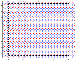
Figure 1: Configuration of the one-component system with perfect hexagonal structure. The dotted lines represent the simulation box which is continued periodically in both directions.

Since the crystal is obviously free of defects it is also stress free. Thus the configuration is ready for subsequent straining.

The preparation of the amorphous solid is more involved. Firstly we equilibrate a system with 65% particles A and 35% particles B at a temperature $T=1$ in Lennard-Jones units. This ratio is chosen to avoid crystallization upon cooling. Next we cool the system to $T=10^{-6}$ in steps of $\Delta T=10^{-3}$ until $T=10^{-3}$ and then in one step to the final temperature. The obtained configuration is not necessarily stress free, with particle position denoted by ${\bm{s}}_{i}$ from the set $\{{\bm{s}}_{i})\}_{i=1}^{N}$. Therefore we apply simple shear which for a general strain $\gamma$ is defined by

$${\bm{r}}_{i}={\bm{h}}(\gamma)\cdot{\bm{s}}_{i}\ ,$$ (3)

with the transformation matrix

$${\bf h(\gamma)}=\left(\begin{array}[]{c c}1&\gamma\\ 0&1\end{array}\right).$$ (4)

Note that this transformation is volume preserving.

The configuration with (almost) zero stress is obtained at a strain $\gamma_{0}$; the particle positions at this configuration are denoted by $\{{\bm{r}}_{i}^{0})\}_{i=1}^{N}$,

$${\bm{r}}^{0}_{i}={\bm{h}}(\gamma_{0})\cdot{\bm{s}}_{i}.$$ (5)

Subsequently we strain the initial configuration, either crystalline or amorphous, with additional external affine simple shear. The procedure is as follows: the particle positions change under shear strain from the reference state $\{{\bm{r}}^{0}_{i}\}$ to a new one, denoted $\{{\bm{r}}_{i}\}$, by an affine transformation that is defined by a matrix ${\bf J}$ :

$${\bm{r}}_{i}={\bm{J}}\cdot{\bm{r}}_{i}^{0}.$$ (6)

Here the matrix ${\bf J}$ in Eq. (6) is given by ${\bf J}={\bf h}(\gamma)\cdot{\bf h}^{-1}(\gamma_{0})$. It follows from Eq. (4) that the matrix ${\bm{J}}$ is defined by

$${\bf J(\gamma)}=\left(\begin{array}[]{c c}1&\gamma-\gamma_{0}\\ 0&1\end{array}\right),$$ (7)

where the strain $\gamma_{0}$ corresponds to the deformation from the rectangular simulation box to the reference system.

In the case of amorphous solid the affine transformation Eq. (6) always destroys the mechanical equilibrium. To regain mechanical equilibrium one should allow a non-affine atomic-scale relaxation of the particle positions $\{{\bm{r}}_{i}\}$ (see, e.g., LM06 ). Also for a crystalline solid at finite temperature one should allow this step of non-affine relaxation. At finite temperature this relaxation can be performed by Molecular Dynamics or Monte Carlo methods. In the Monte Carlo protocol one moves the particles randomly and the move is accepted with probability

$$P_{tr}=\min\bigg{[}1,\exp\bigg{(}-\frac{\Delta G}{T}\bigg{)}\bigg{]},$$ (8)

where $G$ is the generalized enthalpy. Under strain control the matrix ${\bm{h}}$ is fixed and the difference of the generalized enthalpy is defined by the difference of the potential energy of the system $U({\bm{h}},\{{\bm{s}}\})$

$$\Delta G = U({\bm{h}}(\gamma),{\bm{s}}_{1},\cdots,{\bm{s}}_{i}^{new},\cdots{\bm{s}}_{N})-$$ (9)

$$U({\bm{h}}(\gamma),{\bm{s}}_{1},\cdots,{\bm{s}}_{i}^{old},\cdots{\bm{s}}_{N}),\hskip 11.38109pt1\leq i\leq N,$$

where the displacement of the particle positions is defined by

$${\bm{s}}^{new}_{i}={\bm{s}}^{old}_{i}+\delta{\bm{s}},\hskip 11.38109pt1\leq i\leq N$$ (10)

with the periodic boundary conditions taken into account. In this equation the $\alpha$ component of the displacement vector of a particle is given by

$$\delta s^{\alpha}=\Delta s_{max}(2\xi^{\alpha}-1),$$ (11)

where $\Delta s_{max}$ is the maximum displacement and $\xi^{\alpha}$ is an independent random number uniformly distributed between 0 and 1.

It follows from Eq. (8) and Eq. (9) that in the limit $T\to 0$ only the configurations with decreasing energy are accepted, i.e., the Monte Carlo process should converge to one configuration with minimal energy. In practice the direct minimization of the energy of a system at zero temperature after every small increase in strain (the athermal quasistatic (AQS) strain control protocol ML04 ; KLLP10 ) is more effective than the stochastic Monte Carlo method.

III Hexagonal lattice

III.1 Thermodynamic instability

The perfect hexagonal structure is shown in Fig. 1. The energy of the system is minimal, $U/N=-2.5388472$, when the distance between neighboring particles is $R_{0}=1.12152$ (at this point the pressure and the internal shear stress are equal to zero) and the dimensionless particle number density is $\rho=0.918$. The dependence of the energy and the shear stress on the shear strain $\gamma$ under the simple shear defined by Eq. (4) is shown in Fig. 2. The elastic shear modulus of the system estimated at small strains is equal $\mu=24.12$. Note that the shear modulus vanishes at the maximal and minimal points of the stress vs. strain curve in the middle panel of Fig. 2.

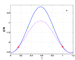
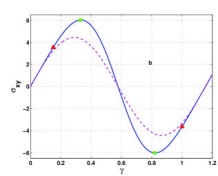
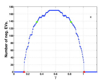
Figure 2: The energy (a) and the shear stress (b) under simple shear. In blue continuous line we represent the exact, numerically computed data. The dashed red line is the Frenkel approximation Eqs. (12) and (13). The red triangle and the green square represent the vibrational and the thermodynamic instabilities respectively. In panel (c) we show the number of negative eigenvalues of the Hessian for the system with $N=400$ as a function of the strain when nonaffine responses are suppressed by hand.

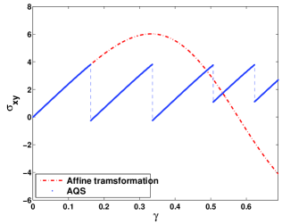
Figure 3: Stress-strain relation for the perfect hexagonal lattice. The solid line shows results of AQS simulatins, dotted line correspond to the affine transformation (see also Fig. 2).

The energy is a periodic function of the strain and reaches its maximum when the hexagonal lattice is transformed into a square one (which is unstable, see, e.g., FHP66 ) at the strain $\gamma=1/\sqrt{(}3)$. It follows from the stress-strain curve (middle panel) that the region between the points indicated by square symbols is thermodynamically unstable. Frenkel proposed an analytical guess for the periodic functions shown in Fig. 2 in the form

$$U=\frac{\mu(1-cos(\sqrt{3}\pi\gamma))}{3\pi^{2}}$$ (12)

and

$$\sigma_{xy}^{int}=\frac{\mu}{\sqrt{3}\pi}sin(\sqrt{3}\pi\gamma)\ .$$ (13)

The Frenkel approximation is shown in Fig. 2 by the dashed lines. Both the approximation and the numerical results indicate that the stress can not exceed some value $\sigma^{int}_{xy}\leq\sigma_{xy}^{Y}$. The quantitative details differ. Eq. (13) yields the estimation $\sigma_{xy}^{Y}=\mu/(\sqrt{3}\pi)\approx\mu/5$, underestimating the result of direct numerical calculation $\sigma_{xy}^{Y}\approx\mu/4$. In fact, Eq. (12) and Eq. (13) should be considered as first terms in a Fourier expansion L55 . The maximum value of the stress in the approximation given by Eq. (13) corresponds to the inflection point of the strain-energy curve at $\gamma_{Y}=1/(2\sqrt{3})$ which is associated with theoretical (ideal) strength which is achieved by a homogeneous deformation.

III.2 Vibrational instability

III.2.1 Pure affine straining

In fact, it is possible to lose stability during purely affine straining due to inhomogeneous deformations by vibrational modes before becoming thermodynamically unstable. The signifiers of such an instability are the eigenvalue of the Hessian matrix. At low temperatures the energy of a system in the solid state can be written in the harmonic approximation

$$U=U_{0}+\Delta r_{i}^{\alpha}H_{ij}^{\alpha\beta}\Delta r_{j}^{\beta}\ ,$$ (14)

with repeated indices summed upon and $\alpha$,$\beta$ denoting the cartesian components. Here $U_{0}$ is the energy of a system in equilibrium and the Hessian ${{\bm{H}}}$ is the matrix

$$H^{\alpha\beta}_{ij}=\frac{\partial^{2}U}{\partial r^{\alpha}_{i}\partial r^{\beta}_{j}}.$$ (15)

In a canonical form Eq. (14) reads

$$U=U_{0}+\sum\limits_{i}\lambda_{i}S_{i}^{2},$$ (16)

where $\lambda_{i}$ are eigenvalues of the Hessian and $S_{i}$ are normal coordinates. It follows from Eq. (16) that in the harmonic approximation a solid can be expressed as a number of uncoupled oscillators. The structure is stable for arbitrary $S_{i}$ if all eigenvalues are positive. The unstable deformation begins when the smallest eigenvalue approaches zero L98 ; ML99 ; MK00 ; GPL01 ; CKCM03 ; KUT04 .

The first eigenvalue $\lambda_{P}$ crosses zero before the shear modulus vanishes, at the value of strain $\gamma_{P}$ denoted with the red triangle in Fig. 2. Note that when the strain increases this eigenvalue becomes negative, and other eigenvalues cross zero and add up to a group of negative eigenvalues. The dependence of the number of the negative eigenvalues on the strain under affine transformation is shown in Fig. 2 lower panel. The hexagonal lattice loses its stability as a harmonic system much before the loss of thermodynamic stability. The reader should note that in practice one would never observe this increase in the number of negative eigenvalues since the system will respond to the instability with non-affine responses that are studied next. Here such non-affine effects were suppressed by hand.

For the perfect crystal without defects we expect the Hessian to be an analytic function of $\gamma$ at least until the point of instability. In other words, we can write

$$<{\bm{\Psi}}_{p}|{\bm{H}}|{\bm{\Psi}}_{p}>\equiv\lambda_{P}=A(\gamma_{P}-\gamma)+B(\gamma_{P}-\gamma)^{2}+\cdots\ ,$$ (17)

where ${\bm{\Psi}}_{P}$ is the eigenfunction of the Hessian associated with the eigenvalue $\lambda_{P}$ that vanishes when $\gamma\to\gamma_{P}$. The consequences of this analyticity assumption are explored below.

III.2.2 Relaxational effects

The picture obtained with purely affine straining is incomplete. For more precise and detailed information it is necessary to take into account relaxational effects in which the system responds to the vanishing of an eigenvalue with non-affine motion. To this aim we apply to the same crystalline hexagonal solid an athermal quasi-static protocol in which after every increase $\Delta\gamma$ in the affine strain we follow up with gradient energy minimization to regain mechanical equilibrium ML04b .

The strain-stress relation obtained in the frame of the AQS protocol is shown in Fig. 3. One sees that the system loses stability before the point of the homogeneous instability. It is useful to follow the trajectory of the lowest eigenvalue of the Hessian matrix as the strain is increased. This is shown in Fig. 4 for two system sizes with $N=400$ and $N=1600$.

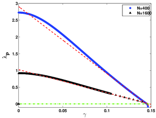
Figure 4: Lowest eigenvalues of the Hessian for a perfect hexagonal lattice with particle number $N=400$ and $N=1600$ in the simulation box. The dashed red lines are an aid to the eye to observe the linearity of the dependence of the eigenvalue on the strain.

The point at which the eigenvalue vanishes is the same for two system sizes. Near this instability point the dependence of $\lambda$ on $\gamma$ is well represented by a linear law. This linearity is a direct consequence of the analyticity assumption (17). This will be shown to be in marked difference from the amorphous solid case.

When the harmonic approximation is being lost it is necessary to take into account effects of anharmonicity in modelling the energy. The simplest model of an anharmonic well is given by

$$U(s)=\frac{1}{2}\lambda_{P}(\gamma)S^{2}+\frac{1}{6}KS^{3},$$ (18)

where $\lambda_{P}(\gamma)$ is the lowest eigenvalue of the Hessian and $K$ is the constant of the anharmonicity. The dependence of the energy given by Eq. (18) on the variable $S$ for different $\lambda_{P}(\gamma)$ is shown in Fig. 5.

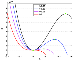
Figure 5: Unharmonic model as given by Eq. (18). The green triangles denote the extrema of the potential.

It follows from Eq. (18) (see also Fig. 5) that the potential barrier is related to the eigenvalue by

$$\Delta U(\gamma)=\frac{2}{3}\frac{\lambda_{P}(\gamma)^{3}}{K^{2}}$$ (19)

One should note that Eq. (18) is only approximate, taking into account only the most unstable mode. In reality, especially in the thermodynamic limit, we expect other modes to intervene and dress the predictions discussed above. This can be seen for example from the fact that the first instability shown in Fig. 3 occurs at $\gamma\approx 0.15$. On the other hand the eigenvalue $\lambda_{P}$ goes to zero at $\gamma\approx 0.14$. Due to the intervention of other modes the eigenvalue should become “slightly negative” before stability is actually lost. To understand this further consider Eq. (16). Upon the energy minimization after the affine step all eigenvalues are effected, some of them increase and some decrease. The positive ones add to Eq. (16) positively and defer the actual instability. If the energy minimization were performed precisely along the critical eigenfunction of the Hessian this slight discrepancy would disappear.

III.3 Monte Carlo studies at finite temperature

Monte Carlo simulations are done at finite temperature, be it as small as it may. This blurs to some extent the definition of the critical strains associated with the instabilities, since temperature fluctuation assist in crossing potential barrier. Thus all the critical values discussed in this section should be understood as upper bounds. It is always possible that longer Monte Carlo runs can result in lower value of the critical strains.

Instantaneous values of the internal shear stress under strain control Monte Carlo simulations are shown in Fig. 6. For values of the strain less than some critical value the stress fluctuates near a given average value. For some critical value of the strain the system dwells for some time in a metastable state and then loses stability, transforming to a new stable state. We chose the critical value of the strain corresponding to the appearance of metastable states.

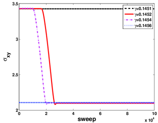
Figure 6: Instantaneous values of the internal shear stress under strain control for different values of the applied strain.

Results of the Monte Carlo protocol for the mean values of the energy and shear stress are shown for the crystal in Fig. 7. Under strain control the system undergoes a series of transitions associated with a loss of stability. Along each elastic branch the system follows the affine transformation (with the strain increased by some value $\gamma-\gamma_{P}$), see Fig. 2). Each elastic branch is ending by a drop at different values of the strain but with the same value of the energy and stress. This values indicate the limit of the stability of the hexagonal lattice. With increasing temperature the critical strains decrease.

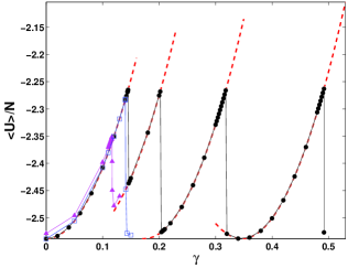
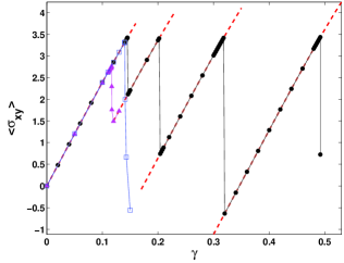
Figure 7: The Monte Carlo results for the energy (upper panel) and the shear stress (lower panel) dependence on the strain for different temperatures. Circles correspond to simulations at $T=10^{-6}$, squares to $T=10^{-4}$ and triangles to $T=10^{-2}$.

At finite temperatures the barrier can be overcome if $T\sim\Delta U$, therefore, the critical value of the eigenvalue is given by

$$\lambda_{P}(\gamma_{P})\sim\bigg{(}\frac{3K^{2}T}{2}\bigg{)}^{1/3}.$$ (20)

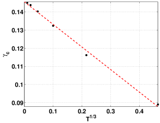
Figure 8: Temperature dependence of the critical value of the strain for the perfect crystal.

The dependence of the lowest eigenvalue of the Hessian (for two system sizes) on the strain estimated in the frame of AQS is shown in Fig. 4. The consequence of the analyticity assumption Eq. (17) is that in the vicinity of the point $\gamma_{P}$ defined by $\lambda_{P}(\gamma_{P})=0$ this dependence can be approximated by the linear function $\lambda_{P}(\gamma)=A(\gamma_{P}-\gamma)$. Substitution of this expression to Eq. (20) yields

$$\gamma_{{}_{Y}}\simeq\gamma_{{}_{Y}}^{0}-C_{1}T^{1/3}.$$ (21)

Results of Monte Carlo indicate the correctness of this assessment (see Fig. 8).

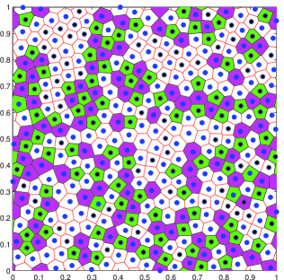
Figure 9: Voronoi diagram for a glass configuration. The color code is green for pentagons, white for hexagons and majenta for heptagons. Sometime an edge in the Voronoi cell can hard to visualize at the scale of this image.

IV Model glass

A composition of $A$ and $B$ particles that is stable in two-dimensions against crystallization is chosen to be $65\%$ of particles $A$ and $35\%$ of particles $B$ BOPK09 . The structure of the configuration of the binary mixture which produces our model glass is shown in Fig. 9.

The typical stress-strain relation of the model glass calculated in the frame of the AQS method is shown in Fig. 10. In contrast to the hexagonal lattice (see Fig. 3) instabilities are now appearing at different values of the stress. This results from the fact that the hexagonal lattice has only one reference state, in the glass there are many reference states and the transition between them is caused by a saddle-node bifurcation that is accompanied by a sudden drop in stress.

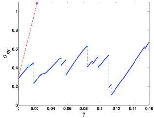
Figure 10: AQS stress-strain relation for a glass. The serrated line corresponds to AQS simulations with non-affine corrections, the dotted line shows stress-strain relation for a purely affine transformation (without non-affine corrections; the first points of instability is indicated by triangles.

The fine structure of the stress-strain relation in the vicinity of the end of an elastic branch is shown in Fig. 11. One can see that there are two special points. One of them corresponds to the vanishing of the elastic modulus followed by the instability point where the lowest eigenvalue of the Hessian goes to zero. It was shown in ML04 that the lowest eigenvalue of the Hessian tends to zero as $\lambda_{P}\sim\sqrt{\gamma_{P}-\gamma}$, where $\gamma_{P}$ denotes the value of the strain at the instability point. When the system is not too large and the lowest eigenvalue is well separated from the larger eigenvalues of the Hessian matrix it follows from this result (which is supported by the simulations) that the elastic modulus in the critical region is approximated by

$$\mu\approx\mu_{B}-\frac{A}{\sqrt{\gamma_{P}-\gamma}},$$ (22)

where $\mu_{B}$ is the Born term. It follows from Eq. (22) that a theory for the glassy state in the spirit of the Frenkel approach would employ for the stress an analytic function in the variable $x=\sqrt{\gamma_{P}-\gamma}$. If applicable, the dependence of the stress on strain could be expanded in Taylor expansion around the point $\gamma_{P}$ KLLP10

$$\sigma_{xy}(\gamma)=\sigma_{P}+\sum\limits_{i=1}c_{i}(\gamma_{P}-\gamma)^{i/2},$$ (23)

where $c_{2}=\mu_{B}$. In fact this expansion may not exist and higher order term may diverge in the thermodynamic limit due to the accumulation of small eigenvalues of the Hessian (prevalence of many low lying barriers), as demonstrated in Ref. 11HKLP

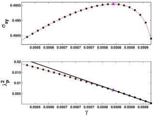
Figure 11: The shear stress (upper panel) and lowest eigenvalue of the Hessian (bottom panel) dependence on the applied strain for a glass configuration. Note that in this case the point A (denoted by the triangle) where the shear modulus vanishes precedes point B where the Hessian lowest eigenvalue $\lambda_{P}$ goes to zero.

IV.1 The difference between crystal and glass

Both for the hexagonal lattice and the glass there is a point of instability defined by a vanishing shear elastic modulus (point A). Another instability point (point B), related to vanishing the lowest eigenvalue of the Hessian appears before point A in the stress-strain dependence of the hexagonal lattice but after point A in the case of glass. This difference has the following consequence: in the case of the hexagonal lattice when the strain is lower than point A the system is thermodynamically stable, and there will be no important difference between stress-controlled and strain-controlled protocols. In both cases the stress can be equilibrated in the system such that in stress-controlled protocols the internal and the external stress are equal. Accordingly one can expect a similar temperature dependencies for $\gamma_{{}_{Y}}(T)$ under stress or strain control.

In contrast, in a glass under stress-control protocols the vanishing of the shear modulus is defined by point A with the lowest eigenvalue of the Hessian being still finite. Therefore, imagine that we apply to the glass a stress-controlled protocol with the external stress being smaller than the critical stress at point A. At this situation the systems is still experiencing a barrier that needs to be overcome since $\lambda_{P}\neq 0$. At $T=0$ therefore we will not experience an instability.

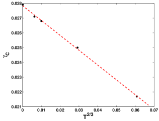
Figure 12: Dependence of the critical strain value on the temperature for a glass.

The temperature dependence of the strain critical value obtained in the frame of the Monte Carlo protocol is shown in Fig. 12. The temperature dependence of the yield strain is in agreement with $\sim T^{2/3}$ behavior JS05 ; DJHP13 .

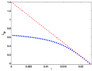
Figure 13: The dependence of the lowest eigenvalue of the Hessian on the applied strain for a glass configuration under affine transformation.

V Conclusion

We have presented highly accurate numerical simulations to underline some fundamental difference between the instabilities of glassy materials and perfect crystals, even when the atomistic interaction are the same. The results indicate the importance of examining small systems where the precise profiles of the stress vs. strain curves can be visualized. Increasing the system size results in reducing the strain or stress differences between points of instability, and eventually obliterating the details of the precise form of the stress vs strain characteristics.

Fundamentally, the difference is in the analytical dependence of the eigenvalues of the Hessian matrix on the strain (or the stress). We note for example Fig. 10, where we highlight the distinction between straining the system allowing non affine response and not allowing it. In the first case the eigenvalue has a square-root singularity as a function of the strain, as discussed in Sect. IV. In the second case, cf. the dotted linear in Fig. 10, the lowest eigenvalue of the Hessian matrix vanishes in an analytic fashion, liner in the strain, much in the same way as in the crystalline case, cf. Fig 13. The avoidance (by hand) of the saddle-node instability of the non affine response results in a fundamental change in the analytics of the dependence of the stress on the strain.

References

- (1) J. Frenkel, Zur Theorie der Elastizitätsgrenze und der Festigkeit kristallinischer Körper. Z. Phys. 37, 572-609 (1926).
- (2) P. Steinman, A. Elizondo and R. Sunyk, Modelling Simul. Mater. Sci. Eng. 15, S271 (2007).
- (3) W. Kob, H. C. Andersen, Scaling behavior in the -relaxation regime of a supercooled Lennard-Jones mixture. Phys. Rev. Lett. 73 1376-1379 (1994).
- (4) V. Dailidonis, V. Ilyin, P. Mishra, I. Procaccia, Mechanical properties and plastisity of a model glass loaded under stress control. Phys. Rev. E90, 052402 (2014).
- (5) A. Lemaître, C. Maloney, Sum rules for the quasistatic and visco-elastic respones of disordered solids at zero temperature. J. Stat. Phys. 123, 415-453 (2006).
- (6) C. Maloney, A. Lemaître, Universal breakdown of elasticity at the onset of material failure. Phys. Rev. Lett. 93, 195501 (2004).
- (7) S. Karmakar, A. Lemaître, E. Lerner, I. Procaccia, Predicting plastic flow events in athermal shear-strained amorphous solids. Phys. Rev. Lett. 104, 215502 (2010).
- (8) A. L. Fetter, P. C. Hohenberg, P. Pincus, Stability of a lattice of superfluid vortices. Phys. Rev. 147, 140-152 (1966).
- (9) G. Leibfried, Gittertheorie der mechanischen und thermischen eigenschaften der kristalle, Handbuch der physik. aspringer-Verlag (1955).
- (10) D. J. Lacks, Localized Mechanical Instabilities and Structural Transformations in Silica Glass under High Pressure. Phys. Rev. Lett. 80, 5385-5388 (1998).
- (11) D. L. Malandro, D. J. Lacks, Relationships of shear-induced changes in the potential energy landscape to the mechanical properties of ductile glasses. J. Chem. Phys. 110, 4593-4601 (1999).
- (12) J. W. Morris Jr., C. R. Krenn, The internal stability of an elastic solid. Phil. Magazine 80, 2827-2840 (2000).A
- (13) G. Gagnon, J. Patton, D. J. Lacks, Energy landscape view of fracture and avalanches in disordered materials. Phys. Rev. E 64, 051508 (2001).
- (14) D. M. Clatterbuck, C. R. Krenn, M. L. Cohen, J. W. Morris, Jr., Phonon Instabilities and the Ideal Strength of Aluminum. Phys. Rev. Lett. 91, 135501 (2003).
- (15) T. Kitamura, Y. Umeno, N. Tsuji, Analytical evaluation of unstable deformation criterion of atomic structure and its application to nanostracture. Comp. Mat. Sci. 29, 499-510 (2004).
- (16) C. Maloney, A. Lemaître, Subextensive scaling in the athermal, quasistatic limit of amorphous matter in plastic shear flow. Phys. Rev. Lett. 93, 016001 (2004).
- (17) R. Brüning, D. A. St-Onge1, S. Patterson, W. Kob, Glass transitions in one-, two-, three-, and four-dimensional binary Lennard-Jones systems. J. Phys.: Condens. Matter 21, 035117 (2009).
- (18) W. L. Johnson, K. Samwer, “A universal criterion for plastic yielding of metallic glasses with a temperature dependence.” Phys. Rev. Lett. 95, 195501 (2005).
- (19) R. Dasgupta, A. Joy, H. G. E. Hentschel, I. Procaccia, “Derivation of the Johnson-Samwer temperature dependence of the yield strain in metallic glasses.” Phys. Rev. B 87, 020101(R) (2013).
- (20) H.G.E. Hentschel, S. Karmakar, E. Lerner and I. Procaccia, “Do Athermal Amorphous Solids Exist?”, Phys. Rev. E 83, 061101 (2011).