A latent variable model with mixed binary and continuous response variables

Abstract

We propose a method for obtaining maximum likelihood estimates in a model with continuous and binary outcomes. Combinations of left and right censored observations are also naturally modeled in this framework. The model and estimation procedure has been implemented in the R package lava.tobit.

The method is demonstrated on brain imaging and personality data where measurement error on predictor variables is handled in a latent variable framework. A simulation study is conducted comparing the small sample properties of the MLE with a limited information estimator.

1 Introduction

Correlated binary data appears in a wide range of applications in psychometrics and epidemiology, including questionnaire studies, longitudinal studies, and cross-sectional studies with multivariate measurements. Depending on the application, different methods have been introduced to model such data. Sometimes marginal effects are of primary interest in epidemiology, in which case inference based on generalized estimating equations (GEE) (Liang and Zeger, 1986) is preferable, and consistent estimates and standard errors are obtained without the need for explicit modeling of the variance structure of the outcomes. In scale validation studies (based on Item Response Theory), and for certain types of matched analyses such as matched case-control studies, inference based on the conditional maximum likelihood (CML) (Andersen, 1971) offers several advantages due to its computational simplicity and the minimal required assumptions on the distribution of the random effects. However, when the assumptions for the CML are not fulfilled, or when interest lies in conditional (subject specific) effects or quantification of the actual variance components, other methods are needed.

A vast amount of literature and software has been written to deal with this situation. The main challenge here is that the likelihood function is given as an integral with respect to the random effects and a numerical approximation to this intractable integral is generally required. Approximate integrated likelihood methods have been proposed via Adaptive Gaussian Quadrature (AGQ) (Pinheiro and Chao, 2006), and various variants of the Expectation-Maximization-algorithm such as Monte Carlo EM (MCEM) (Wei and Tanner, 1990; McCulloch, 1997; Song and Lee, 2005) and Stochastic Approximation EM (SAEM) (Meza and Foulley, 2009). Also Bayesian methods have been popularized with the implementation of general Gibbs-samplers (Gilks et al., 1994; Plummer, 2003).

The dominating framework in applied statistics, however, seems to be the AGQ framework, which is implemented in most widely used software packages such as stata GLLAMM (Rabe-Hesketh et al., 2004), lme4 in R (Bates et al., 2014), and SAS PROC NLMIXED (SAS Institute Inc., 2002-2005). In contrast most Monte Carlo methods are based on more experimental implementations, where ad hoc decisions on e.g. convergence has to be made. An attractive alternative is available via the limited information estimator proposed by Muthén (Muthén, 1984) which generalizes classical structural equation models to allow for inclusion of binary outcomes modeled via a Probit link.

Our model is based on the same principles as (Muthén, 1984). An equivalent model formulation is a threshold model where the responses are generated by underlying normal latent variables. This leads to a generalization of tetrachoric correlations, where we allow conditioning on both covariates and random effects. Numerical approximations is here limited to evaluations of orthant probabilities of the multivariate normal distribution and with computational complexity that is independent of the number of random effects in the model. This is in contrast to the AGQ, where the complexity grows exponentially in the number of latent variables (the curse of dimensionality).

2 The model

Let $Y_{ij}$ be a binary observation. The Probit model can be formulated as a threshold model (see Figure 1), where we assume the existence of an underlying conditionally normally distributed variable $Y_{ij}^{*}$ such that

$$Y_{ij}=\begin{cases}1,&Y_{ij}^{*}>0\\ 0,&Y_{ij}^{*}\leq 0.\end{cases}$$ (1)

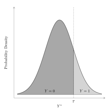
Figure 1: Univariate threshold model with probability of event for the observed binary variable $Y$ given by $\mathbb{P}(Y=1)=\mathbb{P}(Y^{*}>\tau)$. For the bivariate case $\mathbb{P}(Y_{1}=1,Y_{2}=1)=\mathbb{P}(Y_{1}^{*}>\tau_{1},Y_{2}^{*}>\tau_{2})$.

We will let the underlying latent structure be described by a general Linear Latent Variable Model (LLVM), which can be translated into a measurement part describing the latent responses, $Y_{ij}^{*}$:

$$\begin{split}Y_{ij}^{*}&=\nu_{j}+\sum_{k=1}^{l}\lambda_{jk}\eta_{ik}+\sum_{r=1}^{q}\kappa_{jr}X_{ir}+\sum_{k=1}^{l}\delta_{jk}V_{ijk}\eta_{ik}\\ &\qquad\qquad+\varphi^{(j)}_{\bm{\theta}}(X_{i1},\ldots,X_{iq})+\epsilon_{ij},\end{split}$$ (2)

given covariates $X_{ir},V_{ijk}$, and a structural part describing the random effects

$$\begin{split}\eta_{is}&=\alpha_{s}+\sum_{k}^{l}\beta_{sk}\eta_{ik}+\sum_{r=1}^{q}\gamma_{ir}X_{ir}+\sum_{k}^{l}\tau_{sk}W_{isk}\eta_{ik}\\ &\qquad\qquad+\psi^{(s)}_{\bm{\theta}}(X_{i1},\ldots,X_{iq})+\zeta_{ik},\end{split}$$ (3)

with individuals $i=1,\ldots,n$ (between clusters observations), measurements $j=1,\ldots,p$ (within cluster observations) and covariates $W_{isk}$ and random effects $\eta_{ik},k=1,\ldots,l$. For continuous observations we simply let $Y_{ij}=Y_{ij}^{*}$. Notice the interaction term $\delta_{jr}V_{ijr}\eta_{ir}$ defines random slope components and differentiate the LLVM from the a classic Structural Equation Model formulation where the conditional variance of the responses given covariates is assumed to be constant between individuals. Also the functions $\smash{\varphi_{\bm{\theta}}^{(j)}}$ and $\smash{\psi_{\bm{\theta}}^{(s)}}$ allows for non-linear effects of the covariates parameterized by $\bm{\theta}$. The random effects and residual terms $\epsilon$ and $\zeta$ are assumed to follow normal distributions, thus making the likelihood of the observed variables available in explicit form. We will in details describe how to evaluate the likelihood and score function of this model, and we will compare the performance of our method to the limited information estimator (Muthén, 1984). The method is implemented in the open-source R package lava.tobit (Holst, 2012).

3 Estimation method

In the following subsections we will derive the likelihood and the score function for a Gaussian latent variable model under censoring. The Probit model for dichotomous outcomes follows immediately as a special case.

3.1 Right censored data

We first derive a multivariate extension of the Tobit regression model for right censored normal distributed variables (Tobin, 1958), and we later show that this model immediately extends to the more general latent variable framework.

Let $\bm{Y}\in\mathbb{R}^{p}$ be a multivariate censored response, i.e. there exists an underlying variable $\bm{Y}^{*}$ and random censoring times $\bm{C}=(C_{1},\ldots,C_{p})^{\prime}$, such that

$$Y_{j}=\begin{cases}Y_{j}^{*},&Y_{j}^{*}<C_{j}\\ C_{j},&Y_{j}^{*}\geq C_{j}.\end{cases}$$ (4)

For a realization of $\bm{Y}$, we will partition the vector into $\bm{y}=(\bm{y}_{1}^{\prime},\bm{y}_{0}^{\prime})^{\prime}$ where $\bm{y_{1}}\in\mathbb{R}^{m}$ are fully observed and $\bm{y_{0}}\in\mathbb{R}^{k}$ are actually censored components of $\bm{Y_{0}}^{*}$. We will assume that $\bm{Y}^{*}$ follows a normal distribution $\mathcal{N}(\bm{\xi}_{\theta},\bm{\Omega}_{\theta})$. In a common setup, we will also wish to condition on a set of covariates, $(\bm{X},\bm{V},\bm{W})$, but we will omit these here without loss of generality to avoid unnecessarily complex notation.

Let $\bm{\rho}=(\rho_{1},\ldots,\rho_{k})^{\prime}$, and define the set

$$\smash{{}^{\ominus}{\bm{\rho}}=\bigotimes_{i=1}^{k}]-\infty,\rho_{i}]}\quad\text{and}\quad\smash{{}^{\oplus}{\bm{\rho}}=\bigotimes_{i=1}^{k}[\rho_{i},\infty[}.$$ (5)

Now the likelihood contribution (with a somewhat sloppy notation w.r.t joint and conditional probability densities) of a single observation is given by:

$$f_{\bm{\theta}}(\bm{y}_{1},\bm{y}_{0})=\int_{{}^{\oplus}{\bm{y_{0}}}}\varphi_{\bm{\theta}}(\bm{y}_{1},\bm{u})\,d\bm{u}=\varphi_{\bm{\theta}}(\bm{y}_{1})\int_{{}^{\oplus}{\bm{y_{0}}}}\varphi_{\bm{\theta}}(\bm{u}\mid\bm{y}_{1})\,d\bm{u}.$$ (6)

Obviously different individuals will typically have different patterns of censoring, i.e. the partitioning of $\bm{Y}$ will be different, and hence to calculate the log-likelihood of a complete data-set, summing over the log-likelihood contributions of the different patterns of censoring is necessary.

In the following let $\varphi_{\bm{\mu},\bm{\Sigma}}$ and $\Phi_{\bm{\mu},\bm{\Sigma}}$ denote the density and CDF, respectively, of the multivariate normal distribution with mean $\bm{\mu}$ and variance $\bm{\Sigma}$ (with $\varphi_{\bm{0},\bm{\Sigma}}=\varphi_{\bm{\Sigma}}$ and $\Phi_{\bm{0},\bm{\Sigma}}=\Phi_{\bm{\Sigma}}$.).

In the case of no censoring the score is given by

$$\begin{split}\mathcal{S}(\theta;\bm{y})&=-\frac{1}{2}\Big{\{}\left(\frac{\partial\operatorname{vec}\bm{\Omega}_{\theta}}{\partial\bm{\theta}^{\prime}}\right)^{\prime}\Big{(}\operatorname{vec}(\bm{\Omega}_{\theta}^{-1})\\ &\qquad-\operatorname{vec}\left[\bm{\Omega}_{\theta}^{-1}(\bm{y}-\bm{\xi}_{\theta})^{\otimes 2}\bm{\Omega}_{\theta}^{-1}\right]\Big{)}\\ &\qquad+2\left(\frac{\partial\operatorname{vec}{\bm{\xi}_{\theta}}}{\partial\bm{\theta}^{\prime}}\right)^{\prime}\bm{\Omega}_{\theta}^{-1}(\bm{y}-\bm{\xi}_{\theta})\Big{\}}.\end{split}$$ (7)

In the censored case, the derivative of the first term in the log-likelihood corresponding to $\bm{Y}_{1}$

$$S_{1}(\bm{\theta};\bm{y})=\frac{\partial}{\partial\bm{\theta}}\log\varphi_{\bm{\theta}}(\bm{y}_{1})$$ (8)

is easily obtained from (7) by extracting the relevant sub-matrices of $\bm{\xi}_{\theta}$ and $\bm{\Omega}_{\theta}$ and their derivatives, and it follows that

$$\mathcal{S}(\bm{\theta};\bm{y}) =S_{1}(\bm{\theta};\bm{y}_{1})+\frac{\partial}{\partial\bm{\theta}^{\prime}}\log\Phi_{\bm{-\bm{\mu}_{\theta}},\bm{\bm{\Sigma}_{\theta}}}(-\bm{y}_{0})$$ (9)

$$=S_{1}(\bm{\theta};\bm{y}_{1})+\frac{1}{\Phi_{\bm{-\bm{\mu}_{\theta}},\bm{\bm{\Sigma}_{\theta}}}(-\bm{y}_{0})}\frac{\partial}{\partial\bm{\theta}^{\prime}}\Phi_{\bm{-\bm{\mu}_{\theta}},\bm{\bm{\Sigma}_{\theta}}}(-\bm{y}_{0}),$$ (10)

where $\bm{\mu}_{\theta}$ and $\bm{\Sigma}_{\theta}$ are the mean and variance of the conditional distribution of $\bm{Y}_{0}^{*}$ given $\bm{Y}_{1}=\bm{y}_{1}$.

We partition the mean and variance according to the $(\bm{Y}_{1},\bm{Y}_{0}^{*})$:

$$\bm{\xi}_{\theta}=\begin{pmatrix}\bm{\xi}_{\theta}^{(1)}\\ \bm{\xi}_{\theta}^{(0)}\end{pmatrix}\quad\text{ and }\quad\bm{\Omega}_{\theta}=\begin{pmatrix}\bm{\Omega}_{\theta}^{(1)}&\bm{\Omega}_{\theta}^{(01)}\\ \bm{\Omega}_{\theta}^{(10)}&\bm{\Omega}_{\theta}^{(0)}\end{pmatrix},$$ (11)

hence

$$\bm{\mu}_{\theta}=\bm{\mu}_{\theta}(\bm{y}_{1})=\bm{\xi}_{\theta}^{(0)}+\bm{\Omega}_{\theta}^{(01)}{\bm{\Omega}_{\theta}^{(1)}}{}^{-1}(\bm{y}_{1}-\bm{\xi}_{\theta}^{(1)}),$$ (12)

$$\bm{\Sigma}_{\theta}=\bm{\Omega}_{\theta}^{(0)}-\bm{\Omega}_{\theta}^{(01)}{\bm{\Omega}_{\theta}^{(1)}}{}^{-1}\bm{\Omega}_{\theta}^{(10)},$$ (13)

and it follows that

$$\begin{split}\frac{\partial\operatorname{vec}\bm{\mu}_{\theta}}{\partial\bm{\theta}^{\prime}}&=\frac{\partial\operatorname{vec}\bm{\xi}_{\theta}^{(0)}}{\partial\bm{\theta}^{\prime}}+\left\{(\bm{y}_{1}-\bm{\xi}_{\theta}^{(1)})^{\prime}\bm{\Omega}_{\theta}^{(1)}{}^{-1}\otimes\bm{1}_{k}\right\}\frac{\partial\operatorname{vec}\bm{\Omega}_{\theta}^{(01)}}{\partial\bm{\theta}^{\prime}}\\ &\quad-\left\{(\bm{y}_{1}-\bm{\xi}_{\theta}^{(1)})^{\prime}\bm{\Omega}_{\theta}^{(1)}{}^{-1}\otimes\bm{\Omega}_{\theta}^{(10)}\bm{\Omega}_{\theta}^{(1)}{}^{-1}\right\}\frac{\partial\operatorname{vec}\bm{\Omega}_{\theta}^{(1)}}{\partial\bm{\theta}^{\prime}}\\ &\quad-\bm{\Omega}_{\theta}^{(10)}\bm{\Omega}_{\theta}^{(1)}{}^{-1}\frac{\partial\operatorname{vec}\bm{\xi}_{\theta}^{(1)}}{\partial\bm{\theta}^{\prime}}.\end{split}$$ (14)

$$\begin{split}\frac{\partial\operatorname{vec}\bm{\Sigma}_{\theta}}{\partial\bm{\theta}^{\prime}}&=\frac{\partial\operatorname{vec}\bm{\Omega}_{\theta}^{(0)}}{\partial\bm{\theta}^{\prime}}-(\bm{\Omega}_{\theta}^{(01)}{\bm{\Omega}_{\theta}^{(1)}}{}^{-1}\otimes\bm{1}_{k})\frac{\partial\operatorname{vec}\bm{\Omega}_{\theta}^{(01)}}{\partial\bm{\theta}^{\prime}}\\ &\quad+(\bm{\Omega}_{\theta}^{(01)}{\bm{\Omega}_{\theta}^{(1)}}{}^{-1}\otimes\bm{\Omega}_{\theta}^{(01)}{\bm{\Omega}_{\theta}^{(1)}}{}^{-1})\frac{\partial\operatorname{vec}\bm{\Omega}_{\theta}^{(1)}}{\partial\bm{\theta}^{\prime}}\\ &\quad-(\bm{1}_{m}\otimes\bm{\Omega}_{\theta}^{(01)}{\bm{\Omega}_{\theta}^{(1)}}{}^{-1})\frac{\partial\operatorname{vec}\bm{\Omega}_{\theta}^{(10)}}{\partial\bm{\theta}^{\prime}},\end{split}$$ (15)

To calculate the score, (9), the derivative of the CDF with respect to $\bm{\theta}$ is needed, and the result is given in Lemma 2 below. We will need to define the operators $\bm{\mathcal{V}}_{\bm{\mu},\bm{\Sigma}}\colon\mathbb{R}^{k}\to\mathbb{R}^{k\times k}$ and $\bm{\mathcal{M}}_{\bm{\mu},\bm{\Sigma}}\colon\mathbb{R}^{k}\to\mathbb{R}^{k}$ as

$$[\bm{\mathcal{M}}_{\bm{\mu},\bm{\Sigma}}(\bm{y})]_{i}=\int_{{}^{\ominus}{\bm{y}}}\varphi_{\bm{\mu},\bm{\Sigma}}(\bm{x})(x_{i}-\mu_{i})\,d\bm{x},$$ (16)

$$[\bm{\mathcal{V}}_{\bm{\mu},\bm{\Sigma}}(\bm{y})]_{ij}=\int_{{}^{\ominus}{\bm{y}}}\varphi_{\bm{\mu},\bm{\Sigma}}(\bm{x})(x_{i}-\mu_{i})(x_{j}-\mu_{j})\,d\bm{x}.$$ (17)

Evaluating these quantities are obviously closely related to calculating the moments of a truncated normal distribution. We assume without loss of generality that $\bm{\Sigma}$ is a correlation matrix, and look at a standardized normal distribution $\bm{W}\sim\mathcal{N}(\bm{0},\bm{\Sigma})$, and let $\bm{T}$ be the right-truncated version of $\bm{W}$, such that $\bm{T}$ is equal to $\bm{W}$ on the region ${}^{\ominus}{\bm{y}}$. From (Tallis, 1961) the moment generating function of $\bm{T}$ is

$$m(\bm{t})=\mathbb{E}(\exp^{\bm{t}^{\prime}\bm{T}})=\alpha^{-1}\exp(\tfrac{1}{2}\bm{t}^{\prime}\bm{\Sigma t})\Phi_{\bm{\Sigma}}(\bm{y}-\bm{\Sigma t}),$$ (18)

with normalizing constant $\alpha=\Phi_{\bm{\Sigma}}(\bm{y})$, and hence the first and second moments of $\bm{T}$ are

$$\mathbb{E}(\bm{T})=-\alpha^{-1}\bm{\Sigma}D\Phi_{\bm{\Sigma}}(\bm{y})$$ (19)

$$\mathbb{E}(\bm{T}\bm{T}^{\prime})=\bm{\Sigma}+\alpha^{-1}\bm{\Sigma}H\Phi_{\bm{\Sigma}}(\bm{y})\bm{\Sigma},$$ (20)

with $D$ and $H$ denoting the gradient and hessian operator. To calculate these quantities, we can exploit that for the stochastic variables $(U,V)$ partial derivatives with respect to the first components of the corresponding CDF, $F$, is simply the product of the marginal probability density function of $U$ times the CDF of the conditional distribution of $V$ given $U$, $\partial_{u}F(u,v)=f(u)F(v|u)$. As the conditional distributions of a normal distribution is available in analytical form, the gradient and hessian of $\Phi_{\bm{\Sigma}}$ can explicitly be calculated as functions of the CDF and pdf only. Details can be found in (Tallis, 1961) and (Vaida and Liu, 2009, supplementary). Further, as fast and precise approximations are available for the evaluation of the multivariate normal CDF (Genz, 1992; Genz et al., 2014), the evaluation of the integrals (16) is an achievable task.

Lemma 1.

Assume $\bm{\Sigma}_{\theta}$ has full rank and let $\bm{R}_{\bm{\theta}}=\bm{\Lambda}_{\bm{\theta}}^{-1}\bm{\Sigma}_{\theta}\bm{\Lambda}_{\bm{\theta}}^{-1}$ be the corresponding correlation matrix where $\bm{\Lambda}_{\bm{\theta}}$ is the diagonal-matrix with $\operatorname{diag}(\bm{\Lambda}_{\bm{\theta}})=\operatorname{diag}(\bm{\Sigma}_{\theta})^{1/2}$. Then

$$\bm{\mathcal{M}}_{\bm{\mu}_{\theta},\bm{\Sigma}_{\theta}}(\bm{y}) =-\bm{\Lambda}_{\bm{\theta}}\bm{R}_{\bm{\theta}}D\Phi_{\bm{R}}\left(\bm{\Lambda}_{\bm{\theta}}^{-1}(\bm{y}-\bm{\mu}_{\theta})\right)$$

$$\bm{\mathcal{V}}_{\bm{\mu}_{\theta},\bm{\Sigma}_{\theta}}(\bm{y}) =\Phi_{\bm{\mu},\bm{\Sigma}}(\bm{y})\bm{\Sigma}_{\theta}$$

$$\qquad+\bm{\Lambda}_{\bm{\theta}}\bm{R}_{\bm{\theta}}H\Phi_{\bm{R}}\left(\bm{\Lambda}_{\bm{\theta}}^{-1}(\bm{y}-\bm{\mu}_{\theta})\right)\bm{R}_{\bm{\theta}}\bm{\Lambda}_{\bm{\theta}}.$$

Proof.

Follows immediately by substitution $\smash{\bm{v}=\psi(\bm{u})=\bm{\Lambda}_{\bm{\theta}}^{-1}(\bm{u}-\bm{\mu}_{\theta})}$, noting that $\varphi({}^{\ominus}{\bm{y}})$ is scaled and translated but not rotated. ∎

Lemma 2.

$$\frac{\partial}{\partial\bm{\theta}}\Phi_{\bm{\mu_{\theta}},\bm{\Sigma_{\theta}}}(\bm{y}) =\frac{1}{2}\left(\frac{\partial\operatorname{vec}\bm{\Sigma}_{\theta}}{\partial\bm{\theta}^{\prime}}\right)^{\prime}\Big{[}-\operatorname{vec}(\bm{\Sigma}_{\theta}^{-1})\Phi_{\bm{\mu_{\theta}},\bm{\Sigma_{\theta}}}(\bm{y})+$$

$$\qquad(\bm{\Sigma}_{\theta}^{-1}\otimes\bm{\Sigma}_{\theta}^{-1})\operatorname{vec}\{\bm{\mathcal{V}}_{\bm{\mu}_{\theta},\bm{\Sigma}_{\theta}}(\bm{y})\}\Big{]}+$$

$$\qquad\left(\frac{\partial\operatorname{vec}\bm{\mu}_{\theta}}{\partial\bm{\theta}^{\prime}}\right)^{\prime}\bm{\Sigma}_{\theta}^{-1}\operatorname{vec}\{\bm{\mathcal{M}}_{\bm{\mu}_{\theta},\bm{\Sigma}_{\theta}}(\bm{y})\}$$

Proof.

By the fundamental theorem of calculus

$$\begin{split}\frac{\partial}{\partial\bm{\theta}}\Phi_{\bm{\mu_{\theta}},\bm{\Sigma_{\theta}}}(\bm{y})&=\int_{{}^{\ominus}{\bm{y}}}\frac{\partial}{\partial\bm{\theta}}\varphi_{\bm{\mu_{\theta}},\bm{\Sigma_{\theta}}}(\bm{u})\,d\bm{u}\\ &=\int_{{}^{\ominus}{\bm{y}}}\frac{1}{(2\pi)^{k/2}}\frac{1}{\left|\bm{\Sigma}_{\theta}\right|^{1/2}}\frac{-1}{2}\left(\frac{\partial\operatorname{vec}\bm{\Sigma}_{\theta}}{\partial\bm{\theta}^{\prime}}\right)^{\prime}\\ &\qquad\times\operatorname{vec}(\bm{\Sigma}_{\theta}^{-1})\\ &\qquad\times\exp\left(-\tfrac{1}{2}(\bm{u}-\bm{\mu}_{\theta})^{\prime}\bm{\Sigma}_{\theta}^{-1}(\bm{u}-\bm{\mu}_{\theta})\right)\,d\bm{u}\\ &+\int_{{}^{\ominus}{\bm{y}}}\frac{1}{(2\pi)^{k/2}}\frac{1}{\left|\bm{\Sigma}_{\theta}\right|^{1/2}}\\ &\qquad\times\exp\left(-\tfrac{1}{2}(\bm{u}-\bm{\mu}_{\theta})^{\prime}\bm{\Sigma}_{\theta}^{-1}(\bm{u}-\bm{\mu}_{\theta})\right)\\ &\qquad\times\Big{\{}\frac{1}{2}\left(\frac{\partial\operatorname{vec}\bm{\Sigma}_{\theta}}{\partial\bm{\theta}^{\prime}}\right)^{\prime}\\ &\qquad\times\operatorname{vec}(\bm{\Sigma}_{\theta}^{-1}(\bm{u}-\bm{\mu}_{\theta})^{\otimes 2}\bm{\Sigma}_{\theta}^{-1})\\ &\qquad+\left(\frac{\partial\operatorname{vec}\bm{\mu}_{\theta}}{\partial\bm{\theta}^{\prime}}\right)^{\prime}\bm{\Sigma}_{\theta}^{-1}(\bm{u}-\bm{\mu}_{\theta})\Big{\}}\,d\bm{u},\end{split}$$ (21)

where we have used that

$$\frac{\partial}{\partial\bm{\theta}}\left|\bm{\Sigma}_{\theta}\right|^{-\tfrac{1}{2}}=-\frac{1}{2}\left|\bm{\Sigma}_{\theta}\right|^{-\tfrac{1}{2}}\left(\frac{\partial\operatorname{vec}\bm{\Sigma}_{\theta}}{\partial\bm{\theta}^{\prime}}\right)^{\prime}\operatorname{vec}\left(\bm{\Sigma}_{\theta}^{-1}\right)$$ (22)

and

$$\begin{split}&-\frac{\partial}{\partial\bm{\theta}}\left((\bm{u}-\bm{\mu}_{\theta})^{\prime}\bm{\Sigma}_{\theta}^{-1}(\bm{u}-\bm{\mu}_{\theta})\right)=\\ &\qquad\left(\frac{\partial\operatorname{vec}\bm{\Sigma}_{\theta}}{\partial\bm{\theta}^{\prime}}\right)^{\prime}\operatorname{vec}(\bm{\Sigma}_{\theta}^{-1}(\bm{u}-\bm{\mu}_{\theta})^{\otimes 2}\bm{\Sigma}_{\theta}^{-1})\\ &\qquad+2\left(\frac{\partial\operatorname{vec}\bm{\mu}_{\theta}}{\partial\bm{\theta}^{\prime}}\right)^{\prime}\bm{\Sigma}_{\theta}^{-1}(\bm{u}-\bm{\mu}_{\theta})\end{split}$$ (23)

derived by using standard matrix derivative results (Magnus and Neudecker, 1988).

∎

3.2 Combinations of left and right censored data

The extension to include left censored variables follows almost immediately from the right censored case. As before we let $\bm{Y}\in\mathbb{R}^{p}$ be a multivariate censored response, with underlying normal response $\bm{Y}^{*}\sim\mathcal{N}(\bm{\xi}_{\theta},\bm{\Omega}_{\theta})$, defined from right censoring time points $\bm{C}=(C_{1},\ldots,C_{p})^{\prime}$ and left censoring time points $\widetilde{\bm{C}}=(\widetilde{C}_{1},\ldots,\widetilde{C}_{p})^{\prime}$, such that

$$Y_{j}=\begin{cases}Y_{j}^{*},&\widetilde{C}_{j}<Y_{j}^{*}<C_{j}\\ C_{j},&Y_{i}^{*}\geq C_{j}\\ \widetilde{C}_{j},&Y_{j}^{*}\leq\widetilde{C}_{j}.\end{cases}$$ (24)

Again we will partition an observation into $\bm{y}=(\bm{y}_{1}^{\prime},\bm{y}_{0}^{\prime},\widetilde{\bm{y}}_{0}^{\prime})^{\prime}$, where $\bm{y}_{0}\in\mathbb{R}^{k}$ are actual right censored and $\widetilde{\bm{y}}_{0}\in\mathbb{R}^{l}$ are actual left censored, and we exploit that the conditional distribution of the censored indices in $\bm{Y}$ given the fully observed indices is $\mathcal{N}(\bm{\mu}_{\theta},\bm{\Sigma}_{\theta})$.

We define the diagonal matrix

$$\bm{L}=\bm{1}_{k}\oplus(-\bm{1}_{l})$$ (25)

such that

$$\begin{split}&\int_{{}^{\ominus}{\bm{\bm{y}_{0}}}\times{}^{\oplus}{\bm{\widetilde{\bm{y}}_{0}}}}\varphi_{\bm{\bm{\mu}_{\theta}},\bm{\bm{\Sigma}_{\theta}}}(\bm{u}_{1},\bm{u}_{2})\,d\bm{u}_{1}d\bm{u}_{2}=\\ &\qquad\int_{{}^{\ominus}{\bm{\bm{y}_{0}}}\times{}^{\ominus}{\bm{-\widetilde{\bm{y}}_{0}}}}\varphi_{\bm{\bm{L}\bm{\mu}_{\theta}},\bm{\bm{L}\bm{\Sigma}_{\theta}\bm{L}}}(\bm{u}_{1},\bm{u}_{2})\,d\bm{u}_{1}d\bm{u}_{2},\end{split}$$ (26)

hence the log-likelihood is given by

$$\log\varphi_{\bm{\bm{\theta}}}(\bm{y}_{1})+\log\Phi_{\bm{\bm{L}\bm{\mu}_{\theta}},\bm{\bm{L}\bm{\Sigma}_{\theta}\bm{L}}}\begin{pmatrix}\bm{y}_{0}\\ -\widetilde{\bm{y}}_{0}\end{pmatrix}$$ (27)

which is identified as the likelihood of right-censored data, and the expression for the score function follows from the previous section, noting that when applying Lemma 2, we use that

$$\frac{\partial\operatorname{vec}\bm{L}\bm{\Sigma}_{\theta}\bm{L}}{\partial\bm{\theta}^{\prime}}=\bm{L}^{\otimes 2}\frac{\partial\operatorname{vec}\bm{\Sigma}_{\theta}}{\partial\bm{\theta}^{\prime}},$$ (28)

$$\frac{\partial\operatorname{vec}\bm{L}\bm{\mu}_{\theta}}{\partial\bm{\theta}^{\prime}}=\bm{L}\frac{\partial\operatorname{vec}\bm{\mu}_{\theta}}{\partial\bm{\theta}^{\prime}}.$$ (29)

We have not explicitly covered the situation with random effects in the model (as in (2)) but the observed data likelihood follows immediately from the marginalization property of the normal distribution. Assume that $\bm{y}=(\bm{y}_{1},\bm{y}_{0})$ are fully observed resp. right censored observation from an underlying normal model $f_{\bm{\theta}}(\bm{Y},\bm{\eta})$, with random effects $\bm{\eta}$, then by Fubini’s theorem

$$\begin{split}\mathcal{L}({\bm{\theta}};\bm{y})&=\int_{\mathbb{R}^{k}}\int_{{}^{\oplus}{\bm{y_{0}}}}f_{\bm{\theta}}(\bm{y_{1}},\bm{u},\bm{\eta})\,d{\bm{u}}\,d\bm{\eta}\\ &=\int_{{}^{\oplus}{\bm{y_{0}}}}\int_{\mathbb{R}^{k}}f_{\bm{\theta}}(\bm{y_{1}},\bm{u},\bm{\eta})\,d{\eta}\,d\bm{u}\\ &=\int_{{}^{\oplus}{\bm{y_{0}}}}f_{\bm{\theta}}(\bm{y_{1}},\bm{u})\,d{\bm{u}}\\ &=f_{\bm{\theta}}(\bm{y_{1}})\int_{{}^{\oplus}{\bm{y_{0}}}}f_{\bm{\theta}}(\bm{u}\mid\bm{y_{1}})\,d\bm{u}.\end{split}$$ (30)

The last expression is identical to (6) for which we have derived the score.

3.3 Binary responses - the Probit model

The multivariate Probit is trivially handled by noting that all observations are either left censored at $0$ (failure) or right censored at $0$ (event). The probability of observing $\bm{y}=(y_{1},\ldots,y_{p})\in\{0,1\}^{p}$ can therefore be expressed as the orthant probability defined by the model-specific mean and variance

$$\mathbb{P}(\bm{Y}=\bm{y})=\int_{\otimes_{i=1}^{p}(\bm{1}_{\{y_{i}=1\}}-\bm{1}_{\{y_{i}=0\}})]0;\infty[}\varphi_{\bm{\mu},\bm{\Sigma}}(\bm{x})\,d\bm{x}.$$ (31)

In terms of (2) this leads to the model

$$\begin{split}&\mathbb{P}(Y_{ij}=0\mid\bm{X}_{i},\bm{V}_{i},\bm{\eta}_{i})=\Phi\Big{(}\nu_{j}+\sum_{k=1}^{l}\lambda_{jk}\eta_{ik}+\sum_{r=1}^{q}\kappa_{jr}X_{ir}\\ &\qquad\qquad+\sum_{k=1}^{l}\delta_{jk}V_{ijk}\eta_{ik}+\varphi^{(j)}_{\bm{\theta}}(X_{i1},\ldots,X_{ir})\Big{)},\end{split}$$ (32)

where $\Phi$ is the CDF of the standard normal distribution. Hence, in this parameterization we are assuming that the residual terms of $Y_{ij}^{*}$, $\epsilon_{ij}$, $j=1,\ldots,p$ follow a standard normal distribution (not necessarily independent), and the thresholds are fixed at zero as in (1). Other parameterizations are possible, e.g. by constraining $\mathbb{V}\text{ar}(Y_{ij}^{*})=1$, and letting the intercepts of the model be zero.

3.4 Implementation

The maximum likelihood estimates can be obtained via a $BH^{3}$-algorithm (Berndt et al., 1974) or one of several generic optimization routines available in R (R Development Core Team, 2015) (e.g the function nlminb). Letting $\mathcal{S}_{i}(\bm{\theta})$ denote the score contribution of the $i$th individual, we can obtain estimates of the standard errors of the estimates, $\widehat{\bm{\theta}}$, via the information matrix calculated as the outer product of the score

$$\mathcal{I}_{n}(\bm{\theta})=\sum_{i=1}^{n}\mathcal{S}_{i}(\bm{\theta})^{\otimes 2},$$ (33)

also used in the $BH^{3}$-algorithm.

Below we summarize the steps involved in calculating the score function

• For a single observation of responses $\bm{y}_{i}=(y_{i1},\ldots y_{im})^{\prime}$ and covariates $(\bm{x}_{i}^{\prime},\bm{v}_{i}^{\prime})^{\prime}$, and given a set of parameter values, $\bm{\theta}$:

  1. a

  2. b

  3. c

  1. Identify dichotomous responses and redefine failures as left censored at zero, and successes as right censored at zero.

  2. Identify index of observed variables, $\mathcal{I}_{i}$ and censored variables $\mathcal{I}_{i}^{C}$, and let $\bm{y}_{1}=(y_{ij})_{\{j\in\mathcal{I}_{i}\}}$ and $\bm{y}_{0}=(y_{ij})_{\{j\in\mathcal{I}_{i}^{C}\}}$.

  3. Define matrix $\bm{L}$ as in (25), i.e. the diagonal matrix with -1 at entry $i$, if the $i$th coordinate of $\bm{y_{0}}$ is right-censored, and ones on all other diagonal positions.

  4. Calculate model-specific conditional mean $\bm{\xi}_{\theta}$ and variance $\bm{\Omega}_{\theta}$ given covariates, and corresponding partial derivatives, and let $\bm{V}^{\prime}=\frac{\partial\operatorname{vec}\bm{\Omega}_{\theta}}{\partial\bm{\theta}^{\prime}}$ and $\bm{m}^{\prime}=\frac{\partial\operatorname{vec}\bm{\xi}_{\theta}}{\partial\bm{\theta}^{\prime}}$.

  5. For $(\bm{y}_{1},\bm{y}_{0})$ the underlying normal distribution of the fully observed process is partitioned as

     $$\mathcal{N}\left(\begin{pmatrix}\bm{m}_{1}\\ \bm{m}_{0}\end{pmatrix},\begin{pmatrix}\bm{V}_{1}&\bm{V}_{01}\\ \bm{V}_{10}&\bm{V}_{1}\end{pmatrix}\right)$$ (34)

     Calculate the marginal means, $\bm{m}_{1}$, $\bm{m}_{0}$, and variance, $\bm{V}_{1}$, $\bm{V}_{0}$, of $\bm{y}_{1}$, by extracting elements $\mathcal{I}_{i}$. Similarly obtain matrix derivatives $\bm{V}^{\prime}_{1},\bm{V}^{\prime}_{0}$ and $\bm{m}^{\prime}_{1},\bm{m}^{\prime}_{0}$ by extracting the relevant rows from $\bm{V}^{\prime}$ and $\bm{m}^{\prime}$.

  6. Calculate $S_{1}(\bm{\theta})$, the score for $\bm{y}_{1}$, as in equation (7) based on $\bm{V}_{1}$ and $\bm{m}_{1}$

  7. Calculate the conditional mean and variance of the underlying normal distribution of $\bm{y}_{0}$ given $\bm{y}_{1}$

     $$\widetilde{\bm{m}}_{0}=\bm{m}_{0}+\bm{V}_{01}\bm{V}_{0}^{-1}(\bm{y}_{1}-\bm{m}_{1}),$$ (35)

     $$\widetilde{\bm{V}}_{0}=\bm{V}_{0}-\bm{V}_{01}\bm{V}_{0}^{-1}\bm{V}_{10},$$ (36)

     and obtain the derivatives $\widetilde{\bm{m}}_{0}^{\prime}$ and $\widetilde{\bm{V}}_{0}^{\prime}$ as in (15)-(14).

  8. Calculate

     $$S_{2}(\bm{\theta})=\frac{1}{\Phi_{\bm{L}\widetilde{\bm{m}}_{0},\bm{L}\widetilde{\bm{V}}_{0}\bm{L}}(\bm{L}\bm{y}_{0})}\frac{\partial}{\partial\bm{\theta}^{\prime}}\Phi_{\bm{\bm{L}\widetilde{\bm{m}}_{0}},\bm{\bm{L}\widetilde{\bm{V}}_{0}\bm{L}}}(\bm{L}\bm{y}_{0})$$ (37)

     using the results of Lemma (1) and (2) with derivatives

     $$\frac{\partial}{\partial\bm{\theta}^{\prime}}\bm{L}\widetilde{\bm{m}}_{0}=\bm{L}\widetilde{\bm{m}}_{0}^{\prime}\qquad\text{and}\qquad\frac{\partial}{\partial\bm{\theta}^{\prime}}\bm{L}\widetilde{\bm{V}}_{0}\bm{L}=(\bm{L}\otimes\bm{L})\widetilde{\bm{V}}_{0}^{\prime}.$$

  9. Finally calculate the score contribution for the $i$th individual as

     $$\mathcal{S}(\bm{\theta};\bm{y}_{i},\bm{x}_{i},\bm{v}_{i})=S_{1}(\bm{\theta})+S_{2}(\bm{\theta}).$$

   

4 Estimation via composite marginal likelihood

The computational bottleneck of the MLE method is the calculation of the derivatives of the normal CDF based on decomposing the distribution function into all possible combinations of conditional distributions. For the hessian this leads to a computational complexity of order $\mathcal{O}(k^{2})$. To remedy this problem in models with large $k$, we propose to estimate model parameters via composite marginal likelihoods (Lindsay, 1998). We will compound over marginals defined by the index $\mathcal{K}$, and define the composite marginal likelihood as

$$c\ell(\bm{\theta};\bm{y})=\sum_{k\in\mathcal{K}}\ell_{k}(\bm{\theta};\bm{y}^{(k)})$$ (38)

and the corresponding composite score

$$\mathcal{U}(\bm{\theta};\bm{y})=\sum_{k\in\mathcal{K}}\mathcal{U}_{k}(\bm{\theta};\bm{y}^{(k)}),$$ (39)

where $\mathcal{U}_{k}$ is the score corresponding to the marginal log-likelihood $\ell_{k}$. We define

$$\mathcal{I}(\bm{\theta})=\mathbb{E}(-\nabla\mathcal{U}(\bm{\theta};\bm{y}))\quad\text{and}\quad\mathcal{J}(\bm{\theta})=\mathbb{V}\text{ar}(\mathcal{U}(\bm{\theta};\bm{y})).$$ (40)

As we essentially have a mis-specified model, Bartlett’s identity no longer holds ($\mathcal{I}\neq\mathcal{J}$). Instead we can use the Godambe information

$$\mathcal{G}(\bm{\theta})=\mathcal{I}(\bm{\theta})\mathcal{J}(\bm{\theta})^{-1}\mathcal{I}(\bm{\theta}),$$ (41)

and under general regularity conditions the composite likelihood maximizer is asymptotically normally distributed $\sqrt{n}(\widehat{\bm{\theta}}_{cl}-\bm{\theta}^{*})\overset{P}{\rightarrow}\mathcal{N}(\bm{\theta}^{*},G^{-1}(\bm{\theta}^{*}))$, with $\bm{\theta}^{*}$ minimizing the Kullback-Leibler divergence to the marginals of the true model distribution.

In principle the second derivative in $\mathcal{I}$ can be calculated from the results of the previous sections, or it can be approximated numerically. Also Bartlett’s identity holds for each marginal likelihood term, i.e. $\mathcal{I}$ can be calculated as

$$\widehat{\mathcal{I}}=-\frac{1}{n}\sum_{i=1}^{n}\sum_{k\in\mathcal{K}}\mathcal{U}_{k}(\widehat{\bm{\theta}}_{cl};\bm{y}^{(k)}_{i})^{\otimes 2}.$$ (42)

Similarly from the i.i.d. decomposition it follows that the empirical estimator of $\mathcal{J}$ is

$$\widehat{\mathcal{J}}=\frac{1}{n}\sum_{i=1}^{n}\mathcal{U}(\widehat{\bm{\theta}}_{cl};\bm{y}_{i})^{\otimes 2}.$$ (43)

In the composite likelihood approach we can perform the calculations of the derivatives of the CDF for a fixed value $k_{0}$ corresponding to the size of the composite blocks. Using all pairs the growth in the data will be $k(k-1)/2$, and the asymptotic complexity is unchanged. Selecting only neighboring pairs, e.g. $\{(1,2),(2,3),...\}$ will lead to a $\mathcal{O}(n)$-algorithm. For consistency of the composite likelihood estimator, all composite blocks must be correctly specified and the composition must embrace enough of the parameter space in order to identify the parameters of the full joint density.

Generally the loss in efficiency might be compensated by a gain in computational robustness and efficiency. The proposed method of compounding the likelihood of adjacent variables, has been analyzed in a longitudinal setting (Joe and Lee, 2009) showing reasonable power for an auto-regressive correlation structure. In essence this is a limited information estimator but in contrast to (Muthén, 1984), we can in a natural way include incomplete observations in the analysis and make use of the increasing amount of inferential tools invented for composite likelihoods (see (Varin et al., 2011) for a recent overview).

5 Usage

The proposed method for estimation has been implemented in the R package lava.tobit (Holst, 2012) which acts as a plug-in to the package lava (Holst and Budtz-Jørgensen, 2013; Holst, 2015) (an implementation of the LLVM).

As an example we will define a simple structural equation model

$$Y_{ij} =\mu_{j}+\lambda_{j}\eta_{i}+\epsilon_{ij},$$ (44)

$$\eta_{i} =\gamma_{1}X_{1}+\gamma_{2}X_{2}+\zeta_{i}.$$ (45)

with $i=1,\ldots,n;j=1,\ldots,3$, and $\epsilon_{ij}\sim\mathcal{N}(0,\sigma_{j}^{2})$, $\zeta_{i}\sim\mathcal{N}(0,\xi^{2})$. The model is visualized in the path diagram in Figure 2.

Figure 2: Path diagram of structural equation model defined by (44) and (45).

Using the lava-model syntax, this model can be defined in R as

> library(lava.tobit)> m <- lvm()                        # Initialize ’lvm’ model> regression(m) <- c(Y1,Y2,Y3)~eta  # Measurement model> latent(m) <- ~eta                 # Define ’eta’ as random> regression(m) <- eta~X1+X2        # Structural model Various methods for adding (non-linear) parameter constraints and covariance between residual terms of the model exists. We refer to the man-pages of lava for further details.

To simulate 500 observations from the above model, where we dichotomize $Y_{2}$ and introduce fixed right censoring time at 1.5 for $Y_{3}$, we write

> set.seed(1)> d <- transform(sim(m,500),+          Y2=factor(Y2>0),+          Y3=Surv(ifelse(Y3<1.5,Y3,1.5),Y3<1.5)) with intercepts set to 0 and all other parameters 1 (the default parameter values of sim). To find the MLE, the estimate function is used, and since Y2 and Y3 were defined as a factor (with two levels) and as a Surv-object, respectively, the estimate method automatically calculates the likelihood and score function for these parts (Probit and Tobit, respectively) using the described method of Section 3.

> estimate(m,d)

                      Estimate Std. Error    Z value   Pr(>|z|)Measurements:   Y2<-eta           0.8695611  0.0913887  9.5149756     <1e-16   Y3<-eta           1.0169726  0.0472970 21.5018283     <1e-16Regressions:   eta<-X1           1.0039318  0.0588643 17.0550265     <1e-16   eta<-X2           1.0184532  0.0605893 16.8091257     <1e-16Intercepts:   Y2               -0.1033761  0.0869258 -1.1892456  0.2343430   Y3               -0.0480167  0.0688087 -0.6978291  0.4852841   eta              -0.0073254  0.0662993 -0.1104893  0.9120214Residual Variances:   Y1                1.1241819  0.1155639  9.7277922   Y3                0.9106202  0.0987181  9.2244543   eta               1.1072682  0.1221184  9.0671677 To demonstrate the composite likelihood method, we dichotomize Y1, and estimate the parameters of the model using the clprobit function:

> d2 <- transform(d, Y1=factor(Y1>0))> clprobit(m,k=2,data=d2)

                       Estimate  Std. Error     Z value    Pr(>|z|)Measurements:   Y2<-eta           9.5979e-01  1.8883e-01  5.0828e+00  3.7186e-07   Y3<-eta           9.2257e-01  1.4058e-01  6.5627e+00  5.2835e-11Regressions:   eta<-X1           9.9233e-01  1.4059e-01  7.0583e+00  1.6860e-12   eta<-X2           9.1147e-01  3.1514e-01  2.8922e+00  3.8250e-03Intercepts:   Y2               -1.6560e-01  1.0419e-01 -1.5893e+00  1.1199e-01   Y3                7.0581e-02  9.0536e-02  7.7959e-01  4.3563e-01   eta              -1.2235e-01  9.5063e-02 -1.2870e+00  1.9808e-01Residual Variances:   Y3                1.0816e+00  1.5267e-01  7.0847e+00   eta               1.0223e+00  1.6114e-01  6.3442e+00 In this example the block size was 2 and only adjacent variables were compounded, e.g. $(Y_{1},Y_{2})$ and $(Y_{2},Y_{3})$. We refer to the help-page of clprobit on how to customize the blocks used in the composite likelihood estimation (as default continuous non-censored variables will not be split up).

6 Simulation study

In this section we will conduct a comparison between the limited information estimator (LIE) proposed in (Muthén, 1984) and MLE as obtained by our method. We will examine a model (see Figure 3) with a single binary outcome, $Y$, which follows a Probit model given a latent variable $\eta$ and a covariate $X$:

$$\Phi^{-1}\Big{(}\mathbb{P}(Y=0\mid\eta,X)\Big{)}=\mu+\beta_{1}\eta+\beta_{2}X$$ (46)

The latent variable, $\eta$, is measured by 4 continuous variables

$$Z_{j}=\alpha_{j}+\lambda_{j}\eta+\epsilon_{j},\qquad j=1,\ldots,4$$ (47)

and $\eta\sim\mathcal{N}(0,\xi^{2})$, $\epsilon_{j}\sim\mathcal{N}(0,\sigma_{j}^{2})$ are pairwise independent.

Figure 3: Path diagram of structural equation model defined by (46) and (47).

We wish to estimate the effect of two covariates $\eta$ and $X$ on the binary outcome $Y$, which normally would be realizable within the Generalized Linear Model. However, we only have access to indirect measurements of $\eta$, $Z_{1}-Z_{4}$, and using one of these variables as predictor instead of $\eta$ will yield a biased estimate of the effect of $\eta$, due to regression attenuation. The introduction of a measurement model remedies this.

We simulated $n=500$ samples from the model with $X\sim\mathcal{N}(0,1)$, $\lambda_{j}=\sigma_{j}^{2}=\xi^{2}=1$, $\mu=\alpha_{j}=0$, $j=1,\ldots,4$, and the two parameters of primary interest $\beta_{1}=1$ and $\beta_{2}=-0.5$.

Table 1: Simulation study comparing MLE and LIE (Muthén, 1984) based on 10,000 replications of sample-size 500 from the model (3) with $\Phi^{-1}(\mathbb{P}(Y=0\mid\eta,X))=\mu+\beta_{1}\eta+\beta_{2}X$.

		Variance	Rel. Eff.	Bias	MSE	$\frac{\text{Ave(SD}(\widehat{\beta}))}{SD(\widehat{\beta}_{sim})}$
$\mu:$
	MLE	0.0094	1	0.001	0.0094	1.00
	LIE A)	0.0098	0.96	0.001	0.0098	1.03
	LIE B)	0.0099	0.95	0.001	0.0099	1.02
	LIE C)	0.0100	0.94	0.001	0.0100	1.03
	LIE D)	0.0098	0.96	0.001	0.0098	1.03
$\beta_{1}:$
	MLE	0.0128	1	0.020	0.0132	1.00
	LIE A)	0.0139	0.93	0.023	0.0144	1.03
	LIE B)	0.0146	0.88	0.025	0.0152	1.02
	LIE C)	0.0188	0.68	0.030	0.0197	1.03
	LIE D)	0.0139	0.93	0.023	0.0144	1.03
$\beta_{2}:$
	MLE	0.0077	1	-0.009	0.0078	0.99
	LIE A)	0.0123	0.63	-0.009	0.0123	1.02
	LIE B)	0.0087	0.89	-0.011	0.0088	1.01
	LIE C)	0.0163	0.47	-0.015	0.0165	1.03
	LIE D)	0.0083	0.93	-0.010	0.0084	1.01

The MLE and LIE were compared for model (46)-(47) (model A). We also calculated the LIE for the model (model D) where a direct effect of $X$ on $\eta$ was included (the parameter $\beta_{0}$ in Figure 3, a model where a covariance parameter between $\eta$ and $x$ was included (model B), and a model where covariance between the $\eta$ and $x$ was included but fixed to zero (model C). The results of the simulation study based on 10,000 replications are shown in Table 1.

As the MLE asymptotically defines the Cramer-Rao lower-bound, we calculated the relative efficiency as the ratio between the variance of the Monte Carlo parameter estimates of the MLE and the variance of the LIE estimates. For the intercept parameter, $\mu$, all estimators performed well with practically no bias and a relative efficiency of the LIE around 0.95. The LIE of model A and D had a comparable performance with a relative efficiency of 0.93 for the parameter $\beta_{1}$. Remarkably the LIE of model C performed significantly worse, even though it should be equivalent with model A. This might be an implementation artifact. With a sample-size of $n=500$ we still saw a little bias for the parameter $\beta_{1}$ (smallest for the MLE). For $\beta_{2}$ the bias of all estimators was acceptable, but to our surprise the LIE for the true model (A) performed much worse than model D (relative efficiency 0.93) and B (relative efficiency 0.89).

The performance of the estimates of the standard errors of the parameters was quantified by calculating the ratio between the average standard error estimate and the standard deviation of the Monte Carlo parameter estimates. The standard error estimates generally performed acceptable for both the LIE and MLE (calculated via the outer product of the score). Perhaps there is a tendency towards the standard errors from the LIE being a little too conservative.

Overall we can conclude that model D, where the structural model was modeled as $\eta=\beta_{0}X+\zeta$, yielded the best results for the LIE even under the model $\beta_{0}=0$. While clearly outperformed by the MLE, the loss in efficiency might for some applications be out-weighted by a gain in computational efficiency of the LIE. On the other hand, the lack of access to likelihood ratio testing, profile likelihood confidence intervals, the ability to handle incomplete observations, etc., might render this option less attractive.

All simulations were conducted in Mplus version 5.1 (Muthén and Muthén, 2007) and lava.tobit version 0.4-7 (Holst, 2012).

7 Application

In this section we will demonstrate the modeling framework on brain imaging and personality data. Understanding the relationship between personality and biological processes in the brain is recognized as being an important step towards understanding the etiology of mental disorders such as schizophrenia and depression. Dysfunction of the serotonin (5-hydroxytryptamine (5-HT)) $\text{5-HT}_{\text{2A}}$ receptors is considered involved in the development of such disorders (Williams et al., 1996; Choi et al., 2004), thus motivating the search for personality traits associated with the serotonergic system.

Cloninger (Cloninger, 1987) developed the Temperament and Character Inventory (TCI) personality model with a biological interpretation derived from animal studies. The TCI scale is based on dichotomous questionnaires which are summarized into personality traits describing different patterns of behavior such as Harm Avoidance, Reward Dependence and Novelty seeking. It was originally hypothesized that the neurotransmitter systems were related uniquely to specific traits, for instance Harm avoidance and the serotonergic system. However, it has later been proposed that the serotonergic system could be related to regulation of other personality traits (Paris, 2005) as suggested by both genetic and imaging studies (Ebstein et al., 1997; Goethals et al., 2007). The trait Reward Dependence ($RD$) characterizes how a person reacts to reward or punishment. It also seems that serotonin plays an active role for how people reacts towards reward. For example, animal studies have shown that decreased serotonin levels cause more frequent impulsive choices (Bizot et al., 1999; Mobini et al., 2000).

In this study we therefore wanted to examine the relationship between measurements of the serotonergic system in the human brain and the trait Reward Dependence. A Danish translation of the self-administered TCI-R questionnaire (Cloninger, 1994) was answered by 170 subjects. Reward Dependence is traditionally quantified as the sum of three sub-dimensions Sentimentality ($RD_{1}$, 10 questions), Attachment ($RD_{3}$, 8 questions), and Dependence ($RD_{4}$, 6 questions). Each of the sub-dimensions are calculated as the sum of the related dichotomous questions. As a preliminary exercise, we examined the underlying factor structure that justifies the use of these summary statistics. The requirements of criterion related construct validity (Rosenbaum, 1989) are uni-dimensionality, monotonicity and local independence (conditional independence given the latent variable) as illustrated in (56)

(56)

with

$$\Phi^{-1}\Big{(}\mathbb{P}(Y_{i}=0|\eta)\Big{)}=\mu_{i}+\lambda_{i}\eta.$$ (57)

Evidence against this model structure was tested with a likelihood ratio test against the saturated model with a free mean and correlation structure. The factor analysis of $RD_{1}$ and $RD_{3}$ indicated some problems with these scales and we therefore focused on $RD_{4}$. One question (number 71) had to be removed from the analysis due to too little variation causing numerical instability. Three individuals had incomplete observations, which was handled in the MLE approach by ignoring the missing data mechanism under a missing at random assumption (Little and Rubin, 2002). The $\chi^{2}$ omnibus-test yielded a p-value of $0.58$ thus not showing any evidence against the suggested factor structure. For a reliable scale, we would further expect all factor loadings to be equal (after appropriate coding of the questions). A likelihood ratio test against this model yielded a p-value of $0.61$. This suggests that $RD_{4}$ is a valid scale. The dimension Dependence has also previously been shown to be a valid and reliable scale in a sample of hospitalized and ambulant Danish psychiatric patients (Thorleifsson et al., 2010). In the subsequent analyses, we therefore used the suggested factor structure for $RD_{4}$ with equal factor loadings.

Our aim was to quantify the association between central 5-HT function and the trait Dependence. Unfortunately it is not possible to measure brain 5-HT levels directly in vivo. However, several studies have demonstrated a (negative) linear relationship between brain 5-HT levels and 5-HT2A receptor binding (Günther et al., 2008; Cahir et al., 2007), suggesting that low 5-HT leads to compensatory up-regulation of 5-HT2A receptor binding. We therefore proposed a measurement model where $\text{5-HT}_{\text{2A}}$ receptor binding potential measurements were perceived as indirect measurements of underlying global 5-HT level:

$$-{\text{5-HT}_{\text{2A}}}_{,j}=\mu_{j}+\lambda_{j}\cdot\text{5-HT}+\epsilon_{j}.$$ (58)

$\text{5-HT}_{\text{2A}}$ receptor binding potential potential (${\text{BP}_{p}}$) was quantified by Positron Emission Tomography (PET) techniques and segmented into summary statistics of anatomically defined regions (Svarer et al., 2005). For our analysis we chose three regions of interest which previously have been shown to yield reliable quantification of $\text{5-HT}_{\text{2A}}$ receptor binding: Superior frontal cortex (sfc), Anterior cingulate gyrus (acg), and Posterior cingulate gyrus (pcg) (see Figure 4). Effects of age and BMI have previously been demonstrated and was therefore added to the structural model (with BMI dichotomized as overweight (BMI>25) vs non-overweight):

$$\text{5-HT}\propto\text{5-HT}_{\text{2A}}=\gamma_{1}\cdot\text{Age}+\gamma_{2}\cdot\text{BMI}+\zeta.$$ (59)

We conducted an analysis of 56 subjects who completed the TCI questionnaire and also underwent PET examination of the $\text{5-HT}_{\text{2A}}$ receptor binding potential. We refer to the paper (Erritzoe et al., 2010) for a description of this PET sample and details on the methodology. The measurement model for the $\text{5-HT}_{\text{2A}}$ receptor measurements was combined with the measurement model of Dependence (see (56)). The two measurement models were linked with a regression between the two latent variables

$$\mathbb{E}(RD_{4}\mid\text{5-HT}_{\text{2A}})=\beta\cdot\text{5-HT}_{\text{2A}},$$ (60)

leading to the model described in the path-diagram of Figure 4.

Figure 4: Structural equation model describing the association between $\text{5-HT}_{\text{2A}}$ receptor binding potential and Reward Dependence.

The parameters of the model were estimated with MLE as described in Section 3. In the analysis we had to remove one additional item from the measurement model of $RD_{4}$ (question number 131) to avoid numerical instability.

The regression coefficient $\beta$ is interpreted as the linear effect of the underlying $\text{5-HT}_{\text{2A}}$ receptor binding potential level on the latent personality trait Dependence. This interpretation becomes clearer using the standardized coefficient, which we estimated to a increase of 0.791 standard deviation in Dependence caused by increasing the $\text{5-HT}_{\text{2A}}$ receptor binding potential levels one standard deviation (p-value 0.04). Hence high $\text{5-HT}_{\text{2A}}$ receptor binding levels (low 5-HT levels) are associated with higher values of Dependence (more sensitive and socially dependent individuals).

Figure 5: Probabilities of answering yes to different questions of the Dependence personality trait, with varying levels of latent 5-HT levels as measured by $\text{5-HT}_{\text{2A}}$ receptor binding potential. The x-axis is measured in standard deviations away from the mean (reference: non-overweight, age 36).

The model also allows us estimate the conditional probabilities of the answers to the different questions given the 5-HT levels. For instance, for the first question in the $RD_{4}$, we have

$$\mathbb{P}(Y_{1}=1\mid\text{5-HT}_{\text{2A}})=\Phi(0.42+1\cdot 0.42\text{5-HT}_{\text{2A}}).$$

See Figure 5. Similarly the joint probability of different combinations of questions could be evaluated. Also, to obtain a better understanding of the 5-HT/$\text{5-HT}_{\text{2A}}$ receptor effect, we can calculate the probability ratio of answering positively to the first question, for a subject with average $\text{5-HT}_{\text{2A}}$ receptor levels and a subject with $\text{5-HT}_{\text{2A}}$ receptor levels two standard deviations away from the average, $2\cdot\text{SD}(\text{5-HT}_{\text{2A}}\mid Age,BMI)=0.96$,

$$\frac{\mathbb{P}(Y_{1}=0\mid\text{5-HT}=0.96)}{\mathbb{P}(Y_{1}=0\mid\text{5-HT}=0)}=1.20$$

indicating a 20% higher probability of answering positively to question 1 for the subject with high levels of $\text{5-HT}_{\text{2A}}$ receptor binding potential (95% confidence limits by the Delta method: $[1.05;1.34]$).

8 Conclusion

Various methods for estimating parameters in models with correlated multivariate binary data has been proposed. Monte Carlo based methods such as the MCEM algorithm and Bayesian methods are possible, but convergence can be slow and monitoring of the convergence of the Markov chains to the stationary distribution and assessment of the influence of prior distributions in the Bayesian context remains controversial topics. Deterministic integration such as AGQ also suffers from ad hoc decisions which must be made regarding the number of quadrature points to achieve a reasonable approximation. For complex models with many latent variables, it is well-known that this approach may break down in practice.

Our method restricts itself to models with a Probit link, and we have demonstrated how this leads to an algorithm, which allows us to perform fast and precise evaluations of the score and likelihood function of the model. Implementation of generalizations to estimators based on score equations such as Inverse Probability Weighting should therefore follow immediately. In contrast for methods based on applying the Laplace approximation or AGQ where numerical derivatives of the integrated log-likelihood typically is used to approximate the score function, such generalizations could prove much more difficult. Our proposal is most well-suited for models with a moderate number of observed items and possible very complex latent structure. However, the composite likelihood approach scales well with dimension in both number of items and latent variables, and may serve as an important framework for the estimation of complex structural equation models with non-normal response variables.

A strong feature of our model is the possibility of combining continuous, dichotomous and censored observations in a simultaneous model. This may serve as an important framework for the examination of causality (Ditlevsen et al., 2005).

The model has been implemented in full generality in the lava and lava.tobit packages (Holst, 2012) available freely on http://r-forge.r-project.org.

9 Acknowledgments

This work was supported by The Danish Agency for Science, Technology and Innovation.

References

- Andersen (1971) Andersen, E. B., 1971. The asymptotic distribution of conditional likelihood ratio tests. Journal of the American Statistical Association 66 (335), pp. 630–633.
-
Bates et al. (2014)
Bates, D., Maechler, M., Bolker, B., Walker, S., 2014. lme4: Linear
mixed-effects models using eigen and s4 classes.
URL http://arxiv.org/abs/1406.5823 - Berndt et al. (1974) Berndt, E., Hall, B., Hall, R., Hausman, J., 1974. Estimation and inference in nonlinear structural models. Annals of Economic and Social Measurement 3, 653–665.
- Bizot et al. (1999) Bizot, J., Le Bihan, C., Puech, A. J., Hamon, M., Thiebot, M., Oct 1999. Serotonin and tolerance to delay of reward in rats. Psychopharmacology (Berl.) 146, 400–412.
- Cahir et al. (2007) Cahir, M., Ardis, T., Reynolds, G. P., Cooper, S. J., Mar 2007. Acute and chronic tryptophan depletion differentially regulate central 5-HT1A and 5-HT2A receptor binding in the rat. Psychopharmacology (Berl.) 190, 497–506.
- Choi et al. (2004) Choi, M., Lee, H., Lee, H., Ham, B., Cha, J., Ryu, S., Lee, M., 2004. Association between major depressive disorder and the -1438A/G polymorphism of the serotonin 2A receptor gene. Neuropsychobiology 49 (1), 38–41.
- Cloninger (1987) Cloninger, C. R., 1987. A systematic method for clinical description and classification of personality variants. a proposal. Archives of General Psychiatry 44 (6), 573–588.
- Cloninger (1994) Cloninger, R., 1994. The temperament and character inventory (TCI): A guide to its development and use. St. Louis, MO: Center for Psychobiology of Personality, Washington University.
- Ditlevsen et al. (2005) Ditlevsen, S., Christensen, U., Lynch, J., Damsgaard, M. T., Keiding, N., 2005. The mediation proportion: A structural equation approach for estimating the proportion of exposure effect on outcome explained by an intermediate variable. Epidemiology 16 (1), 114–120.
- Ebstein et al. (1997) Ebstein, R., Segman, R., Benjamin, J., Osher, Y., Nemanov, L., Belmaker, R., 1997. 5-HT2C (HTR2C) serotonin receptor gene polymorphism associated with the human personality trait of reward dependence: interaction with dopamine D4 receptor (D4DR) and dopamine D3 receptor (D3DR) polymorphisms. American journal of medical genetics 74, 65–72.
- Erritzoe et al. (2010) Erritzoe, D., Holst, K. K., Frokjaer, V. G., Licht, C. L., Kalbitzer, J., Nielsen, F. A., Svarer, C., Madsen, J., Knudsen, G. M., 2010. A nonlinear relationship between cerebral serotonin transporter and 5-HT2A receptor binding: An in vivo molecular imaging study in humans. Journal of Neuroscience 30 (9), 3391–3397.
-
Genz (1992)
Genz, A., 1992. Numerical computation of multivariate normal probabilities.
Journal of Computational and Graphical Statistics 1 (2), 141–149.
URL http://dx.doi.org/10.1080/10618600.1992.10477010 -
Genz et al. (2014)
Genz, A., Bretz, F., Miwa, T., Mi, X., Leisch, F., Scheipl, F., Hothorn, T.,
2014. mvtnorm: Multivariate Normal and t Distributions. R package version
1.0-2.
URL http://CRAN.R-project.org/package=mvtnorm - Gilks et al. (1994) Gilks, W., Thomas, A., Spiegelhalter, D., 1994. A language and program for complex bayesian modelling. The Statistician, 169–178.
- Goethals et al. (2007) Goethals, I., Vervaet, M., Audenaert, K., Jacobs, F., Ham, H., de Wiele, C. V., Vandecapelle, M., Slegers, G., Dierckx, R., van Heeringen, C., 2007. Differences of cortical 5-HT2A receptor binding index with SPECT in subtypes of anorexia nervosa: Relationship with personality traits? Journal of Psychiatric Research 41 (5), 455 – 458.
- Günther et al. (2008) Günther, L., Liebscher, S., Jahkel, M., Oehler, J., Sep 2008. Effects of chronic citalopram treatment on 5-HT1A and 5-HT2A receptors in group- and isolation-housed mice. Eur. J. Pharmacol. 593, 49–61.
-
Holst (2012)
Holst, K. K., 2012. lava.tobit: Latent variable models with censored and binary
outcomes. R package version 0.4-7.
URL http://lava.r-forge.r-project.org/ -
Holst (2015)
Holst, K. K., 2015. lava: Linear Latent Variable Models. R package version
1.4.
URL http://lava.r-forge.r-project.org/ - Holst and Budtz-Jørgensen (2013) Holst, K. K., Budtz-Jørgensen, E., 2013. Linear latent variable models: the lava-package. Computational Statistics 28 (4), 1385–1452.
- Joe and Lee (2009) Joe, H., Lee, Y., 2009. On weighting of bivariate margins in pairwise likelihood. Journal of Multivariate Analysis 100 (4), 686–698.
- Liang and Zeger (1986) Liang, K.-Y., Zeger, S., 1986. Longitudinal data analysis using generalized linear models. Biometrika 73 (1), 13–22.
- Lindsay (1998) Lindsay, B., 1998. Composite likelihood methods. Contemporary Mathematics 80, 221–240.
- Little and Rubin (2002) Little, R. J. A., Rubin, D. B., 2002. Statistical analysis with missing data, 2nd Edition. Wiley Series in Probability and Statistics. Wiley-Interscience [John Wiley & Sons], Hoboken, NJ.
- Magnus and Neudecker (1988) Magnus, J. R., Neudecker, H., 1988. Matrix differential calculus with applications in statistics and econometrics. Wiley Series in Probability and Mathematical Statistics: Applied Probability and Statistics. John Wiley & Sons Ltd., Chichester.
- McCulloch (1997) McCulloch, C. E., 1997. Maximum likelihood algorithms for generalized linear mixed models. Journal of the American Statistical Association 92 (437), 162–170.
- Meza and Foulley (2009) Meza, Cristian Jaffrézic, F., Foulley, J.-L., 2009. Estimation in the probit normal model for binary outcomes using the saem algorithm. Computational Statistics & Data Analysis 53 (4), 1350 – 1360.
- Mobini et al. (2000) Mobini, S., Chiang, T. J., Al-Ruwaitea, A. S., Ho, M. Y., Bradshaw, C. M., Szabadi, E., Apr 2000. Effect of central 5-hydroxytryptamine depletion on inter-temporal choice: a quantitative analysis. Psychopharmacology (Berl.) 149, 313–318.
- Muthén (1984) Muthén, B. O., 1984. A general structural equation model with dichotomous, ordered categorical and continuous latent indicators. Psychometrika 49, 115–132.
- Muthén and Muthén (2007) Muthén, L. K., Muthén, B. O., 2007. Mplus User’s Guide (Version 5), 5th Edition. Los Angeles, CA: Muthén & Muthén.
- Paris (2005) Paris, J., 2005. Neurobiological dimensional models of personality: a review of the models of cloninger, depue, and siever. Journal of personality disorders 19 (2), 156–170.
- Pinheiro and Chao (2006) Pinheiro, J. C., Chao, E. C., 2006. Efficient laplacian and adaptive gaussian quadrature algorithms for multilevel generalized linear mixed models. Journal of Computational and Graphical Statistics 15 (1), 58–81.
- Plummer (2003) Plummer, M., 2003. JAGS: A program for analysis of bayesian graphical models using gibbs sampling. In: Hornik, K., Leisch, F., Zeileis, A. (Eds.), Proceedings of the 3rd International Workshop on Distributed Statistical Computing, Vienna, Austria.
-
R Development Core Team (2015)
R Development Core Team, 2015. R: A Language and Environment for Statistical
Computing. R Foundation for Statistical Computing, Vienna, Austria, ISBN
3-900051-07-0.
URL http://www.R-project.org/ - Rabe-Hesketh et al. (2004) Rabe-Hesketh, S., Skrondal, A., Pickles, A., 2004. Generalized multilevel structural equation modeling. Psychometrika 69, 167–190.
- Rosenbaum (1989) Rosenbaum, P., 09 1989. Criterion-related construct validity. Psychometrika 54 (4), 625–633.
- SAS Institute Inc. (2002-2005) SAS Institute Inc., 2002-2005. SAS OnlineDoc 9.1.3. Cary, NC: SAS Institute Inc.
- Song and Lee (2005) Song, X.-Y., Lee, S.-Y., 2005. A multivariate probit latent variable model for analyzing dichotomous responses. Statistica Sinica 15, 645–664.
- Svarer et al. (2005) Svarer, C., Madsen, K., Hasselbalch, S. G., Pinborg, L. H., Haugbol, S., Frokjaer, V. G., Holm, S., Paulson, O. B., Knudsen, G. M., 2005. MR-based automatic delineation of volumes of interest in human brain PET images using probability maps. Neuroimage 24, 969–979.
- Tallis (1961) Tallis, G. M., 1961. The moment generating function of the truncated multi-normal distribution. Journal of the Royal Statistical Society. Series B (Methodological) 23 (1), 223–229.
- Thorleifsson et al. (2010) Thorleifsson, A., Holst, K. K., Diaz, M., Folker, H., Feb 2010. Personality test and prediction of antidepressive treatment effect in mental illness. Ugeskr Laeger 172 (7), 539–544, article in Danish.
- Tobin (1958) Tobin, J., 1958. Estimation of relationships for limited dependent variables. Econometrica 26, 24–36.
- Vaida and Liu (2009) Vaida, F., Liu, L., 2009. Fast implementation for normal mixed effects models with censored response. Journal of Computational and Graphical Statistics 18 (4), 797–817.
- Varin et al. (2011) Varin, C., Reid, N., Firth, D., 2011. An overview of composite likelihood methods. Statistica Sinica 21, 5–42.
- Wei and Tanner (1990) Wei, G. C. G., Tanner, M. A., 1990. A monte carlo implementation of the em algorithm and the poor man’s data augmentation algorithms. Journal of the American Statistical Association 85 (411), 699–704.
- Williams et al. (1996) Williams, J., Spurlock, G., McGuffin, P., Mallet, J., Nöthen, M., Gill, M., Aschauer, H., Nylander, P., Macciardi, F., Owen, M., 1996. Association between schizophrenia and T102C polymorphism of the 5-hydroxytryptamine type 2A-receptor gene. european multicentre association study of schizophrenia (EMASS) group. Lancet 347 (9011), 1294–1296.