Optimal Decomposition and Recombination of Isostatic Geometric Constraint Systems for Designing Layered Materials
Abstract
Optimal recursive decomposition (or DR-planning) is crucial for analyzing, designing, solving or finding realizations of geometric constraint sytems. While the optimal DR-planning problem is NP-hard even for general 2D bar-joint constraint systems, we describe an algorithm for a broad class of constraint systems that are isostatic or underconstrained. The algorithm achieves optimality by using the new notion of a canonical DR-plan that also meets various desirable, previously studied criteria. In addition, we leverage recent results on Cayley configuration spaces to show that the indecomposable systems—that are solved at the nodes of the optimal DR-plan by recombining solutions to child systems—can be minimally modified to become decomposable and have a small DR-plan, leading to efficient realization algorithms. We show formal connections to well-known problems such as completion of underconstrained systems. Well suited to these methods are classes of constraint systems that can be used to efficiently model, design and analyze quasi-uniform (aperiodic) and self-similar, layered material structures. We formally illustrate by modeling silica bilayers as body-hyperpin systems and cross-linking microfibrils as pinned line-incidence systems. A software implementation of our algorithms and videos demonstrating the software are publicly available online111Visit http://cise.ufl.edu/~tbaker/drp/index.html..
keywords:
rigidity , geometric constraint solving , configuration spaces , self-similar structures , layered materials1 Introduction
Geometric constraint systems have well-established, mature applications in mechanical engineering and robotics, and they continue to find emerging applications in diverse fields from machine learning to molecular modeling. Solving or realizing geometric constraint systems requires finding real solutions to a large multivariate polynomial system (of equalities and inequalities representing the constraints); this requires double exponential time in the number of variables, even if the type or orientation of the solution is specified. Thus, to realize a geometric constraint system, it is crucial to perform recursive decomposition into locally rigid subsystems (which have finitely many solutions), and then apply the reverse process of recombining the subsystem solutions. With the use of decomposition-recombination (DR-) planning, the complexity is dominated by the size of the largest subsystem that is solved, or recombined, from the solutions of its child subsystems, i.e. the maximum fan-in occurring in a DR-plan. In addition, navigating and analyzing the solution spaces, as well as designing constraint systems with desired solution spaces, leads to the optimal decomposition-recombination (DR-) planning problem [1, 2, 3].
For a broad class of geometric constraint systems, local rigidity is characterized generically as a sparsity and tightness condition of the underlying constraint (hyper)graph [4, 5, 6, 7]. This allows the generic DR-planning problem to be stated and treated as a combinatorial or (hyper)graph problem as we do in this paper.
We additionally conjecture that versions of Frontier, a previously given, bottom-up, polynomial time method for obtaining DR-plans with various desired properties [2, 3, 8, 1], in fact generate an optimal DR-plan for non-overconstrained systems.
Naïvely, the optimal DR-plan is used as follows. Each decomposed subsystem—a node of the DR-plan—is treated and solved as a polynomial system of constraints between its child subsystems. However, even in an optimal DR-plan, there can be arbitrarily many children at a node. In other words, even in the recursive decomposition given by an optimal DR-plan, the size of the maximal indecomposable subsystem could be arbitrarily large. It represents a bottleneck that dictates the complexity of solving or realizing the constraint system [9, 10, 11]. We address this problem using the recently developed concept of convex Cayley configuration spaces [12, 13, 14, 15, 16, 17]. This allows for even greater reduction of the complexity by realizing large, indecomposable systems in a manner that avoids working with large systems of equations. Specifically, we give an efficient technique for optimally modifying large indecomposable subsystems in a manner that reduces their complexity while preserving desired solutions; the modification ensures a convex Cayley configuration space, and the space can be efficiently searched to find a realization that satisfies the additional constraints of the original system. This optimal modification problem is a generalization of the previously studied problem of optimal completion of underconstrained systems [1, 18].
DR-plans are especially useful for constraint systems that exhibit some level of self-similarity and quasi-uniformity, in addition to isostaticity. These properties can be leveraged to further reduce the complexity of both optimal DR-plan construction and recombination. We consider 3 different types of constraint systems—which we collectively call qusecs—that are used to model, design, and analyze quasi-uniform or self-similar materials. In the remainder of this section, we motivate the materials application and give the contributions and organization of the paper.
1.1 Introducing Qusecs
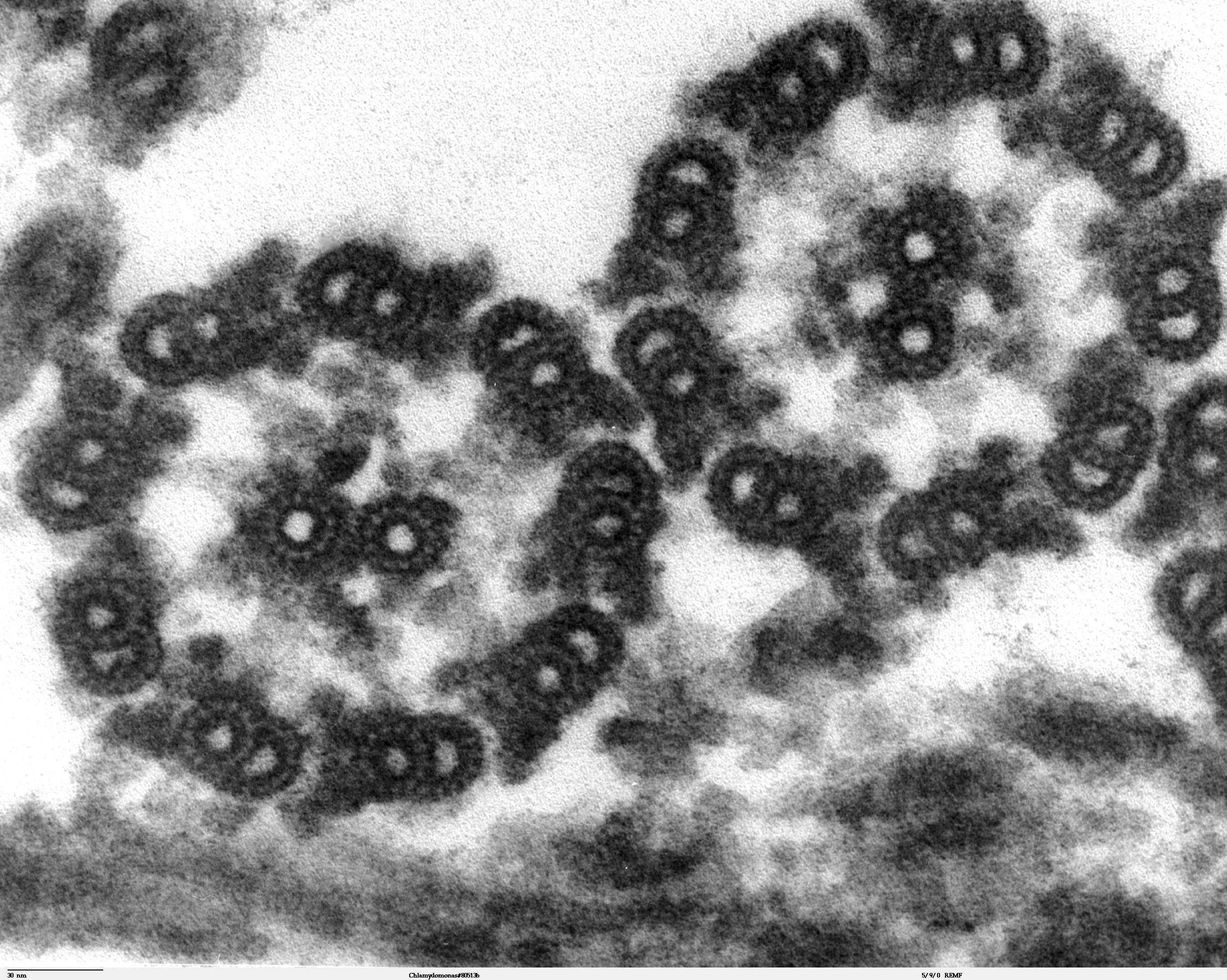
A large class of constraint systems that we call qusecs, a contraction of “quasi-uniform or self-similar constraint system”, (a) can be treated combinatorially as described above and (b) occur as independent (isostatic or underconstrained) systems in materials applications. We discuss these next. Some natural and engineered materials can be analyzed by treating them as two dimensional (2D) layers. As illustrated by the examples below, the structure within each layer is often: self-similar222In this manuscript we only study finite 2D structures. Self-similarity refers to the result of finitely many levels of hierarchy or subdivision in an iterated scheme to generate self-similar structures. [19], spanning multiple scales; generally aperiodic and quasi-uniform within any one scale; and composed of a few repeated motifs appearing in disordered arrangements. Note that a 2D layer is not necessarily planar (genus 0), it can consist of multiple, inter-constraining planar monolayers. Furthermore, a layer is often either isostatic or underconstrained (not self-stressed/overconstrained, see 2.1 for definitions). These properties, as well as quasi-uniformity, aperiodicity, self-similarity, and layered structure, are natural consequences of evolutionary pressures or design objectives such as stability, minimizing mass, optimally distributing external stresses, and participating in the assembly of diverse and multifunctional, larger structures.
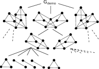
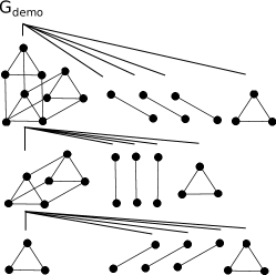
The importance of an optimal DR-plan is particularly evident for a qusecs. The quasi-uniform or self-similar properties mean that the decomposition and solution for one subsystem can be used as the decomposition and solution for other subsystems, thus causing further reduction in the complexity of both DR-planning and recombination. This is shown in Figures 3 and 9.
Some materials that are readily modeled as qusecs include:
- 1.
-
2.
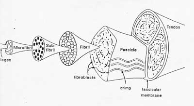
Cross-sections of organic tissue with hierarchical structure, e.g., compact bone and tendon (Figure 1(b)).
- 3.
- 4.
- 5.
1.2 Organization and Contributions
In Section 2, we provide basic definitions in combinatorial rigidity theory, and formalize the new notion of qusecs [9, 10, 11]. In addition, we define DR-plans and what it means for a DR-plan to be complete or optimal. We survey previous work on DR-planning algorithms, discussing other desirable criteria of DR-plans and their relation to the NP-hard optimality property of DR-plans.
In Section 3, we define a so-called canonical DR-plan and prove a strong Church-Rosser property: all canonical DR-plans for isostatic or underconstrained qusecs are optimal. In so doing, we navigate the NP-hardness barrier present in the general form of the DR-planning problem; the canonical DR-plan elucidates the essence of the NP-hardness of finding optimal DR-plans when a system is over-constrained. Furthermore, our optimal/canonical DR-plan satisfies desirable properties such as the previously studied cluster minimality [2]. Also in this section, a polynomial time () algorithm is provided to find a canonical DR-plan for isostatic bar-joint graphs. While this and the next section focus on bar-joint graphs, the theory is easily extended to other qusecs used to model the abovementioned types of materials, as shown in subsequent sections.
In Section 4, we give a method to deal with the algebraic complexity of recombining the realizations or solutions of child subsystems into a solution of the parent system [9, 10, 11]. Specifically, we define the problem of minimally modifying the indecomposable recombination system so that it becomes decomposable via a small DR-plan and yet preserves the original solutions in an efficiently searchable manner. When the modifications are bounded, we obtain new, efficient algorithms for realizing both isostatic and underconstrained qusecs by leveraging recent results about Cayley parameters in [12, 13, 14] (see Sections 4.3 and 4.4). In Section 4.5, we show formal connection to well known problems such as optimal completion of underconstrained systems [18, 1, 34] and to find paths within the connected components.
In Section 5 and 6, we briefly describe applications of the above techniques to modeling, analyzing, and designing specific properties in 2D material layers [35]. We explicitly model these materials as qusecs. For Examples 4 and 5, we discuss boundary conditions for achieving various desired properties of body-hyperpin systems. For Example 3, we discuss canonical and optimal DR-plans for pinned line incidence systems [36].
The last Section 7 concludes the paper, and Section 7.1 lists open problems and conjectures. In particular, we conjecture that the methods of Section 3 extend in fact to a large class of (hyper)graphs, formally those with an underlying abstract rigidity matroid in which independence corresponds to some type of sparsity, and maximal independence (rigidity) is a tightness condition.
Throughout this paper, an asterisk after a formal statement indicates that its proof appears in A.
A software implementation of our algorithms and videos demonstrating the software are publicly available online333See footnote 1..
2 Preliminaries and Background
We first give basic definitions and concepts in combinatorial rigidity, leading to a definition of a DR-plan, its properties, and how they relate. The section ends with a discussion of previous work on DR-plans.
2.1 Geometric Constraint Systems and Combinatorial Rigidity
In this paper, a geometric constraint system is a multivariate polynomial (usually bilinear or quadratic) system , representing constraints with parameters between geometric primitives in represented collectively as . When the type of constraint (system) is fixed, the system is simply represented as , where is the underlying constraint (hyper)graph with the vertices representing the geometric primitives in and (hyper)edges representing the constraints, each with an associated parameter . For example, a bar-joint system or linkage , is a graph with fixed length bars as edges, i.e. ; this represents the distance constraint system for , where represents the coordinates of .
In all types of geometric constraint systems we consider in this paper, a Cartesian realization or solution of is an assignment of coordinates or Euclidean transformations (poses), or , to the vertices of satisfying the constraints with parameters , modulo orientation preserving isometries (Euclidean rigid body motions).
Although the realization space itself depends on the constraint parameters , many relevant generic properties of the constraint system are defined to be properties of the constraint (hyper)graph and do not depend on (or they hold for all but a measure zero set of values). Many of these are properties of the Jacobian , often called the appropriate rigidity matrix of (a matrix of indeterminates). For example, the bar-joint rigidity matrix of the graph is a matrix of indeterminates representing the Jacobian of the distance map for . The matrix has columns per vertex in and one row per edge in , where the row corresponding to edge contains the 2 coordinate indeterminates for (resp. ) in the 2 columns for (resp. ), i.e. 4 non-zero entries per row.
One important property of a generic constraint system or (hyper)graph444We refer to these as properties of the constraint system or as properties of the underlying (hyper)graph interchangeably is rigidity, i.e. the realizations or solutions of the corresponding constraint system being generically isolated and zero-dimensional. The result by Asimow and Roth [37] shows a constraint (hyper)graph is rigid if and only if it is generically infinitesimally rigid, i.e. the number of independent rows of its appropriate rigidity matrix is at least the number of columns less the number of rigid body motions, which is 3 for 2D bar-joint systems.
Geometric constraint systems can also have inequalities in addition to equations, where the parameters in are small intervals rather than exact values. In this case, the definition of rigidity is approximate; the solutions are isolated, small, full-dimensional connected components.
Other generic constraint system or (hyper)graph properties are mentioned here. A constraint (hyper)graph is independent if its appropriate rigidity matrix of indeterminates has independent rows (i.e. the determinant of some square submatrix is not identically zero). It is isostatic (minimally rigid, wellconstrained) if it is both rigid and independent. It is flexible if it is not rigid, underconstrained if it is independent and not rigid, or overconstrained if it is not independent.
Defining the combinatorial independence of a subset of edges to be the independence of corresponding rows in the rigidity matrix of indeterminates, we obtain the rigidity matroid of a constraint (hyper)graph . There are various results on combinatorial characterization of independence, rigidity, and rigidity matroids for different types of (hyper)graphs. For bar-joint rigidity matroids, the famous Laman’s theorem [4] states that the underlying graph is isostatic if and only if and for every induced subgraph with at least 2 vertices. The result by Lovasz and Yemini [38] shows that all 6-vertex-connected graphs are rigid in the plane. For bar-body rigidity matroids, Tay [6] proved that the underlying multigraph is isostatic if and only if it can be decomposed as edge disjoint spanning trees. White and Whiteley [7] gave the same characterization using a different technique to study the algebraic-geometric conditions of genericity, called pure condition. Lee, Streinu and Theran [39] defined the -sparsity matroid, where a hypergraph is called -sparse if for any induced subgraph with at least 2 vertices, and -tight if it is -sparse and . In general, given a -uniform hypergraph, a -sparsity condition is matroidal as long as .
2.2 Decomposition-Recombination (DR-) Plans
Definition 1.
The decomposition-recombination (DR-) plan [2] of graph , , is defined as a forest that has the following properties:
-
1.
Each node represents/contains/is a rigid subgraph of .
-
2.
The children of a node satisfy .
-
3.
A leaf node is a single edge. A trivial graph is empty or a single vertex. Note that a trivial graph is not isostatic.
-
4.
A root node is a vertex-maximal rigid subgraph of .
A DR-plan is complete if it satisfies an additional property: for a non-leaf node , its children are all of the rigid vertex-maximal proper subgraphs of . This makes Property 2 implicit. We denote a complete DR-plan of as .
A DR-plan is optimal if it minimizes the maximum fan-in over all nodes in the tree. The maximum fan-in is called the size of the DR-plan. We denote an optimal DR-plan of as .
Remark 2.
More than one node (leaf) in a DR-plan forest may represent the same subgraph (vertex) of . For a given graph, there could be exponentially many DR-plans—and even optimal DR-plans—in the size of the graph. A complete DR-plan is unique but may not be (and is usually not) optimal. DR-plans of self-similar graphs are self-similar.
2.3 Previous Work on DR-Plans
We now briefly survey existing techniques for detecting rigidity and creating DR-plans of 2D constraint systems. The limitations of these techniques directly motivate the contributions of the next section.
2.3.1 Finding (Vertex)-Maximal, Generically Rigid Subsystems
Fast, graph-based algorithms exist (pebble-game [40, 41, 42, 43]), for locating all maximal, generically rigid subsystems (formally defined in 2.1). When the input itself is rigid, these algorithms do nothing, i.e. compute the identity function.
However, both for self-similar or just aperiodic 2D qusecs, it is imperative to recursively decompose rigid systems into their rigid subsystems, down to the level of geometric primitives, in order to understand or design properties at all scales, such as (formally defined in 2.1) rigidity, flexes, distribution of external stresses, boundary conditions for isostaticity, as well as behavior under constraint variations.
2.3.2 Optimal Recursive Decomposition (DR-Planning)
Recursive decomposition of geometric constraint systems has been formalized [2, 3] and well-studied [8, 1, 42] as the Decomposition-Recombination (DR-) planning problem (formally defined in Section 2.1). For the abovementioned classes of 2D qusecs, generic rigidity is a combinatorial property and hence each level of the decomposition should, in principle, be achievable by a graph-based algorithm without involving the geometric information in the constraint system. Since many such decompositions can exist for a given constraint system, criteria defining desirable or optimal DR-plans and DR-planning algorithms were given in [2].
However, for overconstrained 2D qusecs, even when restricted to bar-joint systems, the optimal DR-planning problem was shown to be NP-hard [8, 1]. The NP-hardness of the optimal DR-planning problem for 2D bar-joint graphs is partly the consequence of possibly exponential number of DR-plans. On the other hand, although the complete DR-plan is unique it could have large average fan-in and exponentially many nodes making it far from optimal.
2.3.3 DR-plans for Special Classes and with Other Criteria
For a special class of 2D qusecs, namely tree-decomposable systems [44, 45, 46] common in computer aided mechanical design (which includes ruler-and-compass and Henneberg-I constructible systems), all DR-plans turn out to be optimal. This satisfies the Church-Rosser property, leading to highly efficient DR-planning algorithms. For general 2D qusecs, alternate criteria were suggested such as cluster minimality requiring parent systems to have a minimal set of at least 2 rigid proper subsystems as children (i.e. the union of no proper subset of size at least 2 child subsystems forms a rigid system); and proper maximality, requiring child subsystems to be maximal rigid proper subsystems of the parent system. See 2.1 for formal definitions.
While polynomial time algorithms were given to generate DR-plans meeting the cluster minimality criterion [8], no such algorithm is known for the latter criterion.
3 Main Result: Canonical DR-Plan, Optimality, and Algorithm
3.1 Canonical DR-Plan
In this section, we define a canonical plan to capture those aspects of an optimal DR-plan that mimic the uniqueness of a complete DR-plan, and we show that the nonunique aspects do not affect optimality for independent (underconstrained or isostatic) graphs. Furthermore, we give an efficient algorithm to find the canonical DR-plan of any independent graph. The definition is as follows:
Definition 3.
The canonical DR-plan of a graph satisfies the following three properties: (1) it is a DR-plan of ; (2) children are rigid vertex-maximal proper subgraphs of the parent; and (3) if all pairs of rigid vertex-maximal proper subgraphs intersect trivially then all of them are children, otherwise exactly two that intersect non-trivially are children.
In this section and in section 4, any reference to a graph is assumed to be isostatic (i.e. well-constrained or -tight).
Definition 3 gives the canonical DR-plan a surprisingly strong Church-Rosser property, which is made explicit in Theorem 4, the main result of this section.
Theorem 4.
A canonical DR-plan exists for a graph and any canonical DR-plan is optimal if is independent.
Proof.
We show the existence of a canonical DR-plan by constructing it as follows:
Begin with of a rigid 2D bar-joint graph , for all nodes with children retain children nodes according to the following rules:
-
1.
If is trivial then retain all as children.
-
2.
If is rigid then select any two out of as children.
This directly satisfies Properties (2) and (3) of a canonical DR-plan (see Definition 3), because all the nodes in are rigid vertex-maximal proper subgraphs, which we shorten to clusters. To show Property (1) holds (that this constitutes a DR-plan): for Case 1 above, since we start with a complete DR-plan, if we preserve all the children it is still a DR-plan; for Case 2 above, we know that the union must be rigid as well and it cannot be anything other than , otherwise we would have found a larger rigid proper subgraph of , contradicting vertex-maximality.
Note that if we begin with an isostatic graph, “rigid” can be replaced with “isostatic” throughout the construction and preserve the above properties. The rigid proper subgraphs of an isostatic graph must be isostatic themselves.
Next we show that a canonical DR-plan is optimal.
First, note that any DR-plan without the Property (2) of a canonical DR-plan can always be modified (by introducing intermediate nodes) to satisfy Property (2) without increasing the max fan-in, since any rigid proper subgraph of a graph (a child of node of the DR-plan ) is the subgraph of some cluster of . Thus without loss of generality, we can assume that an optimal DR-plan satisfies Property (2) of a canonical DR-plan.
The proof of optimality of a canonical DR-plan is by induction on its height. The base case trivially holds for canonical DR-plans of height 0, i.e. for single edges. The induction hypothesis is that canonical DR-plans of height are optimal for the root node. For the induction step consider a canonical DR-plan of height rooted at a node . Notice that represents a canonical DR-plan for the graphs corresponding to each of its descendant nodes. Thus, from the induction hypothesis, we know that the is optimal for .
Thus it is sufficient to demonstrate a set of nodes that must be present in any DR-plan for that satisfies Property (2), including a known optimal one; and furthermore, for any such DR-plan , either (Claim 1) must be the set of children of ; or (Claim 2) for all the ancestors of , has the minimum possible fan-in of 2.
We show the two claims below. The first claim is that for a node whose clusters have trivial pairwise intersections, any DR-plan of that satisfies Property (2) must also satisfy Property (3) at , i.e. the set of children of consists of all clusters of . Because this is the only choice, it is the minimum fan-in at for any DR-plan for with Property (2), including a known optimal one. The second claim shows that in the case of nodes whose rigid, vertex-maximal proper subgraphs have non-trivial pairwise intersections, every canonical DR-plan of that uses any possible choice of two such subgraphs of as children results in a minimum possible fan-in of 2 in the ancestor nodes leading to the same maximal antichain of descendants of . The antichain is maximal in the partial order of rigid subgraphs of under containment. I.e. satisfies the property that every proper vertex-maximal rigid subgraph of is a superset of some in ; this follows from properties of maximal antichains that no element of is contained in the union of other elements of ; and the union of elements of is . Thus any DR-plan that satisfies Property (2) and hence contains two or more of the rigid vertex-maximal proper subgraphs of as children must also contain every element of . The two claims complete the proof that every canonical DR-plan is optimal.
Claim 1: A set of clusters whose pairwise intersection is trivial, must be children of in an optimal DR-plan.
We prove this claim by showing that the union of no subset of the children can be , thereby requiring all of them to be included as children.
We prove by contradiction. Assume to the contrary that the strict subset such that is isostatic. If , then we found a larger proper subgraph contradicting vertex-maximality of the . So, it must be that . However, since is trivial then for we know, by Lemma 6, Item 3, must be one or more trivial, i.e. disconnected vertices. By definition of a DR-plan, and we know that so . Thus, is (i) a collection of disconnected vertices, and (ii) an isostatic subgraph of , which is impossible. As is isostatic, this means the union of no proper subset of is isostatic, nor is it equal to , proving Claim 1.
Furthermore, since a canonical DR-plan has nodes with proper rigid vertex-maximal subgraphs as children, if, as in this case, their pairwise intersection is trivial, it follows that any node has at most as many children as a DR-plan without this restriction, because the union of the children must contain all edges of the parent. Therefore, the canonical DR-plan is the optimal choice in this case of trivial intersections.
Claim 2: If some pair in the set of child clusters of has an isostatic (nontrivial) intersection, then choosing any two as children (minimum possible fan-in) will result in the same maximal antichain of descendants of .
To prove Claim 2, notice that if is isostatic, then, by Observation 5, is also isostatic. This means that, by Lemma 6, Point 2, the union of any two children of is itself. Thus, any two children can be chosen to make a canonical DR-plan and that is the minimum fan-in possible for a node of the DR-plan.
However, to guarantee that any two are the optimal choice, it must ensure minimum fan-in over all descendants leading up to a common maximal antichain of subgraphs.
To prove this holds, take the set , and denote and . Suppose and , where , are the children. For convenience, we will assume all subgraphs are induced subgraphs of . We know that and . The isostatic vertex-maximal subgraphs of are all of whose pairwise intersections are isostatic subgraphs. So any two of these are viable children for . This continues for levels, always with fan-in of two (the minimum possible), at which point every descendant of is some for , with every appearing at least once. At the last level, there are exactly two rigid proper vertex-maximal subgraphs, and hence a unique choice of pair of children. Thus, regardless of the sequence of choices of and , and of their descendants at each level, the DR-plan has the optimal fan-in of two for every node for levels, and the collection of last level nodes contain the same maximal antichain of subgraphs (for all choices). ∎
This proof of this theorem relies on the following crucial observation and lemma. These will be used again in the application sections (5 and 6) of the paper, with modifications to work for other types of qusecs.
Observation* 5.
If and are non-empty isostatic graphs then the following hold:
(1) is not trivial;
(2) is underconstrained if and only if is trivial;
(3) is isostatic if and only if is isostatic; and
(4) is not underconstrained.
The following key properties hold at the nodes of a canonical DR-plan.
Lemma* 6.
Let be an isostatic node of a canonical DR-plan, with distinct children . Assume . Then
-
1.
is isostatic if and only if .
-
2.
If is isostatic, then is isostatic. Alternatively, if , then .
-
3.
If is trivial, then is trivial.
Remark 7.

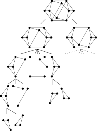
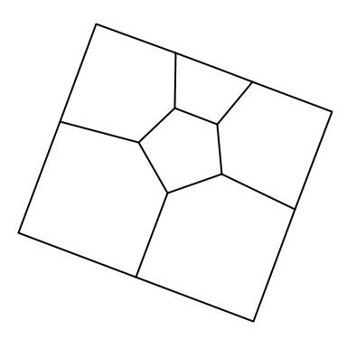
Example 8 (DR-plan for self-similar structure).
This example details the decomposition of the graph in Figure 3, the canonical DR-plan of . It begins with the whole (isostatic) graph as the root. The graph has only two isostatic vertex-maximal subgraphs: without the outermost triangle composed of graphs (triangle ) and without the inner triangle (triangle ). These intersect on without triangle and which is clearly isostatic. As explained in the proof of Theorem 4, since there are only 2 possible children, their intersection must be a node 2 levels below the parent. As expected, it is on the third level, as a child of both of ’s children.
Both of ’s children are similar to , but containing only triangles. Therefore, the canonical DR-plans of these children follow the same pattern. This continues downward until the individual doublets are reached (there will be multiple occurrences of the same doublets at this level, but they can be represented as the same node in a DAG).
Further decomposition of one of these doublets is shown. The three edges between the triangles and the triangles themselves all intersect trivially pairwise. By Theorem 4, part 1, they must all be children in the DR-plan. Similarly, the triangles decompose into their three trivially intersecting ’s. Then the subgraphs decompose into their separate 9 edges.
The self-similar nature of this graph is evident in the canonical DR-plan. Many structures are repeated throughout the DR-plan, allowing for shared computation in both decomposition and recombination.
3.2 Algorithm
Theorem 9.
There exists an algorithm to find a canonical DR-plan for an input graph.
Proof.
We first describe the algorithm. The first step of the algorithm, which we call , is finding the isostatic vertex-maximal proper subgraphs (clusters) of the input isostatic graph . One of many ways to do this is by first dropping arbitrary edge from the edge set and running the pebble game algorithm [40] on this subgraph, which is . The output of this will be a list of cluster-candidates. The next step is to isolate the set of true-clusters by running the Frontier algorithm [3] [8] () on each candidate along with edge , to find the minimal subgraph that contains the candidate and . If , the candidate is moved (before adding ) to the true-cluster list and removed from the candidate-cluster list. If , all candidates that are subgraphs of are removed from the candidate-cluster list and is added back to the list. The next candidate is considered until all candidates are exhausted.
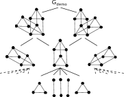
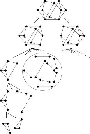
The next step is to check the intersection of any two of the true-components. If the intersection is trivial, the entire list becomes the children, and the algorithm is recursively applied to each child. If the intersection is non-trivial (necessarily isostatic), the decomposition is computed down to . (This is discussed in detail in the proof of Theorem 4). We construct a DR-plan whose node set is that of a canonical/optimal DR-plan. Begin with the parent . Its children are and , where and is , together with all incident edges. Observe that these edges are incident on vertices from and that is underconstrained so its DR-plan is a forest where each root becomes a child of . The children of are and , where and is together with all incident edges. The process iterates. At levels down, the children are and , where is together with all incident edges. Apply the algorithm recursively to both children. Thus we obtain an efficient method for the case of DR-plan nodes whose rigid proper vertex-maximal subgraphs have non-trivial intersections, avoiding recomputation of the isostatic components of . See Figure 4 for an example.
To summarize the above step of the algorithm: if the intersection is trivial, recursively apply to the entire list of true-components and set the resulting trees as the children. Else, the intersection is non-trivial, and the children of the node are and , where is the first true-component of the parent (chosen arbitrarily, could be any child) and is the underconstrained graph formed by together with all incident edges and the associated nodes in .
The DR-plan output by this algorithm is a tree where each node is a distinct subgraph. The leaves of this tree are the edges of the starting graph . Therefore, the number of nodes in the tree is which, for isostatic input graphs, is and the complexity of the algorithm is . ∎
3.3 Overconstrained Graphs and NP-Hardness of Optimal DR-Planning
For overconstrained (not independent) graphs, a canonical DR-plan is still well-defined. However, it may be far from optimal. The proofs of Theorem 4, Observation 5, and Lemma 6 all fail for overconstrained graphs. It is important to note that, regardless whether the graph is overconstrained, if every node in a canonical DR-plan has clusters whose pairwise intersection is trivial, then the DR-plan is the unique one satisfying Property (2), and since we know that there is an optimal DR-plan that satisfies Property (2), is in fact optimal. The problem arises when some node in a DR-plan has clusters whose pairwise intersection is non-trivial. In this case, an arbitrary choice of a pair of clusters as children of an overconstrained node in a canonical DR-plan may not result in an optimal DR-plan. This is in contrast to independent graphs, which, as shown in Theorem 4, exhibit the strong Church-Rosser property that any choice yields an optimal DR-plan. A good source of examples of overconstrained graphs with canonical DR-plans that are not optimal are graphs whose cluster-minimal DR-plans that are not optimal. The example shown in Figure 5 is a canonical, cluster-minimal DR-plan that is not optimal; an optimal DR-plan is also shown in the figure. The root cause of the NP-hardness is encapsulated in this figure: because the different choices of vertex-maximal subgraphs for overconstrained input do not incur the same fan-in, finding the optimal DR-plan becomes a search problem with a combinatorial explosion of options.
As mentioned earlier, the Modified Frontier algorithm version given in [8] runs in polynomial time and finds a cluster-minimal DR-plan for any graph. Similarly, the algorithm given above finds a canonical DR-plan also for any input graph. However neither of these DR-plans may be optimal for overconstrained graphs as shown in Figure 5.
While the canonical DR-plan is optimal only if the input graph is independent, when there are only overconstraints for some fixed , we can still find the optimal DR-plan using a straightforward modification of the above algorithm. However, the time complexity is exponential in .
4 Recombination and Problem Relationships
In this section, we consider the optimal recombination problem of combining specific solutions of subsystems in a DR-plan into a solution of their parent system (without loss of generality, at the top level of the DR-plan). In the case of isostatic qusecs, the parent system is isostatic (the root of the DR-plan), and we seek solution(s) (among a finite large number of solutions) with a specific orientation or chirality. In the case of underconstrained qusecs the subsystems are the multiple roots of the DR-plan, the parent system is underconstrained, and we typically seek an efficient algorithmic description of connected component(s) of solutions with a specific orientation or chirality.
The main barrier in recombination when given an optimal DR-plan (of smallest possible size or max fan-in) for a system , is that the number of children of the root (resp. number of roots of the DR-plan)—and correspondingly the size and complexity of the (indecomposable) algebraic system to be solved—could be arbitrarily large as a function of the size of . This difficulty can persist even after optimal parametrization of the indecomposable system as in [9] to minimize its algebraic complexity.
4.1 Previous Work
We now briefly survey existing techniques for handling the complexity of recombination of DR-plans for qusecs. The limitations of these techniques directly motivate the contributions in this section.
4.1.1 Optimal Recombination and Solution Space Navigation
For the entire DR-plan, finding all desired solutions is barely tractable even if recombination of solved subsystems is easy for each indecomposable parent system in the DR-plan. This is because even for the simplest, highly decomposable systems with small DR-plans, the problem of finding even a single solution to the input system at the root of the DR-plan is NP-hard [47] and there is a combinatorial explosion of solutions [48]. Typically, however, the desired solution has a given orientation type, in which case, the crux of the difficulty is concentrated in the algebraic complexity of (re)combining child system solutions to give a solution to the parent system at any given level of the DR-plan. For fairly general 3D constraint systems, there are algorithms with formal guarantees that uncover underlying matroids to combinatorially obtain an optimal parameterization to minimize the algebraic complexity of the indecomposable parent (sub)systems that occur in the DR-plan [9, 10, 11], provided the DR-plan meets some of the abovementioned criteria.
However, the generality of these algorithms trades-off against efficiency, and, despite the optimization, the best algorithms can still take exponential time in the number of child subsystems (which can be arbitrarily large even for optimal DR-plans) in order to guarantee all solutions of a given orientation type, even for a single (sub)system in a DR-plan. They are prohibitively slow in practice. We note that, utilizing the DR-plan and optimal recombination as a principled basis, high performance heuristics and software exists [49] to tame combinatorial explosion via user intervention.
4.1.2 Configuration Spaces of Underconstrained Systems
For underconstrained 2D bar-joint and body-hyperpin qusecs obtained from various subclasses of tree-decomposable systems, algorithms have been developed to complete them into isostatic systems [18, 1, 34, 12] and to find paths within the connected components [13, 50] of standard Cartesian configuration spaces. Most of the algorithms with formal guarantees leverage Cayley configuration space theory [12, 13, 14] to characterize subclasses of graphs and additional constraints that control combinatorial explosion, and provide faithful bijective representation of connected components and paths. These algorithms have decreasing efficiency as the subclass of systems gets bigger, with highest efficiency for underlying partial 2-tree graphs (alternately called tree-width 2, series-parallel, and minor avoiding), moderate efficiency for 1 degree-of-freedom (dof) graphs with low Cayley complexity (which include common linkages such as the Strandbeest, Limacon, and Cardioid), and decreased efficiency for general 1-dof tree-decomposable graphs. While software suites exist [51, 52, 53, 54], no such formal algorithms and guarantees are known for non-tree-decomposable systems.
4.2 Optimal Modification for Recombination
In the following, we formulate the problem of optimal modification of an indecomposable algebraic system at some node of a (possibly optimal) DR-plan into a decomposable system with a small DR-plan (low algebraic complexity). Leveraging recent results on Cayley configuration spaces, our approach to the optimal modification problem achieves the following:
-
1.
Small DR-plan. We obtain a parameterized family of systems —one for each value for the parameters , all of which have small DR-plans. Thus, given a value for , the system can potentially be solved or realized easily once the orientation type of the solution is known (when the DR-plan size is small enough).
-
2.
Solution preservation. Moreover, the union of solution spaces of the systems in the family is guaranteed to contain all of ’s solutions.
-
3.
Efficient search. Finally, the so-called Cayley or distance parameter space is convex or otherwise easy to traverse in order to search for ’s solution (or connected component) of the desired orientation type. For the case when the modification (number of Cayley parameters) is bounded, this approach provides an efficient algorithm for recombination. We first define the decision version of the problem of optimal modification for decomposition. The standard optimization versions are straightforward.
Optimal Modification for Decomposition (OMD) Problem. Given a generically independent graph with no non-trivial proper isostatic subgraph (indecomposable) and 2 constants and , does there exist a set of at most edges and a set of non-edges such that the modified graph has a DR-plan of size at most ? The OMDk problem is OMD where is a fixed bound (not part of the input). We say that such a tuple is a member of the set OMDk. We loosely refer to graphs as OMD with appropriately small and or OMDk with appropriately small .
It is immediately clear that indecomposable graphs that belong in OMDk for small and lend themselves to modification into decomposable graphs satisfying Criteria (a) and (b) above. However, it is not clear how Criterion (c) is met by OMD graphs. Before we consider this question, we discuss previous work on recombination of DR-plans.
4.3 Using Convex Cayley Configuration Spaces
Next we provide the necessary background to describe a specific approach for achieving the requirements (a)–(c) mentioned above, by restricting the class of reduced graphs and their isostatic completions in the above definition of the OMD problem, and using a key theorem of Convex Cayley configuration spaces [12]. This theorem characterizes the class of graphs and non-edges (Cayley parameters), such that the set of vectors of attainable lengths of the non-edges is always convex for any given lengths for the edges of (i.e. over all the realizations of the bar-joint constraint system or linkage in 2 dimensions). This set is called the (2-dimensional) Cayley configuration space of the linkage on the Cayley parameters , denoted and can be viewed as a “projection” of the cartesian realization space of on the Cayley parameters . Such graphs are said to have convexifiable Cayley configuration spaces for some parameters (short: is convexifiable).
To state the theorem, we first have to define the notion of 2-sums and 2-trees. Let and be two graphs on disjoint sets of vertices and , with edge sets and containing edges and respectively. A 2-sum of and is a graph obtained by taking the union of and and identifying and . In this case, and are called 2-sum components of . A minimal 2-sum component of is one that cannot be further split into 2-sum components. A 2-tree is recursively obtained by taking a 2-sum of 2-trees, with the base case of a 2-tree being a triangle. A partial 2-tree is a 2-tree minus some edges. Partial 2-trees have an alternate characterization as the graphs that avoid minors, and are also called series-parallel graphs.
Theorem 10.
[12] has a convexifiable Cayley configuration space with parameters if and only if for each all the minimal 2-sum components of that contain both endpoints of are partial 2-trees. The Cayley configuration space of a bar-joint system or linkage is a convex polytope. When is a 2-tree, the bounding hyperplanes of this polytope are triangle inequalities relating the lengths of edges of the triangles in .
The idea of our approach to achieve the criteria (a)–(c) begins with the following simple but useful theorem.
Theorem 11.
Given an indecomposable graph , let be a spanning partial 2-tree subgraph in with fewer edges than . Then belongs in the set OMDk.
Proof.
The proof follows from the fact that 2-trees are well decomposable and have simple DR-plans of size 2. We know that can be reduced by removing edges to create a partial 2-tree which can then be completed to an (isostatic) 2-tree by adding some set of non-edges . Thus the modified graph has a DR-plan of size 2, proving the theorem. ∎
We refer to such graphs in short as -approximately convexifiable, where the reduced graphs and isostatic completions are convexifiable. As observed earlier, since graphs such as are in OMDk, Criteria (a) and (b) are automatically met for small enough . Criterion (c) is addressed as described in the following efficient search procedure which clarifies the dependence of the complexity on the number and ranges of Cayley parameters .
Theorem* 12 (Efficient search).
For an indecomposable, -approximately convexifiable graph , let be a spanning partial 2-tree subgraph where . Let be a set of non-edges of such that is a 2-tree. Each solution (or connected component of a solution space) of of an orientation type can be found in time where is the number of cells of desired accuracy (discrete volume) of the convex polytope . The (discrete) volume is exponential in and polynomial in the (discrete range) of the parameters in .


Note: A major advantage of the convex Cayley method is that it is completely unaffected when are intervals of values rather than exact values [12].
Example 13 (Using Cayley configuration space).
A graph cannot be decomposed into any nontrivial isostatic graphs, i.e. its DR-plan has a root and 9 children corresponding to the 9 edges. Solving or recombining the system corresponding to the root of this DR-plan involves solving a quadratic system with 8 equations and variables. Instead of simultaneously solving this system, we could instead use the fact that is in OMD2: remove the edges in Figure 6 to give a partial 2-tree . Now add the non-edges to give a 2-tree with a DR-plan of size 2. The Cayley configuration space is a single interval of attainable length values for the edge . When is generic, i.e. does not admit collinearities or coincidences in the realizations of , the realization space of has 16 solutions (modulo orientation preserving isometries), with distinct orientation types (two orientation choices for each of the 4 triangles) that can be obtained by solving a sequence of 4 single quadratics in 1 variable (DR-plan of size 2). By subdivided binary search in the interval , the desired solution of is found when the length of the nonedge in the realization is .
In fact, we can show that is in OMD1 by removing a single edge to reduce (as shown in Figure 6) to a tree-decomposable graph of low Cayley complexity (which includes the class of partial 2-trees). In the next Section 4.4, we discuss this issue of why the largest class of reduced graphs is desirable.
4.4 Optimized Modification by Enlarging the Class of Reduced Graphs
It is possible in principle to decrease for a OMDk graph (i.e. the number of edges to be removed to ensure an isostatic completion that is decomposable with a small DR-plan) by considering reduced graphs (and modified graphs ) that come from a larger class than partial 2-trees but nevertheless have convex Cayley configuration spaces at least when the realization space is restricted to a sufficiently comprehensive orientation type. In particular, the so-called tree-decomposable graphs of low Cayley complexity [13, 14] include the partial 2-trees and many others that are not partial 2-trees. See an illustration in Figure 6. These too result in DR-plans of size 2 or 3, putting in the class OMDk and thus meeting Criteria (a) and (b). The Criterion (c) is met—for example when —because 1-dof Cayley configuration spaces of linkages based on such graphs are known to be single intervals when a comprehensive orientation type of the sought solution is given. In addition, the bounds of these intervals are of low algebraic complexity. More precisely, the bounds can themselves be computed using a DR-plan of size 2 or 3, i.e. the computation of these bounds is tree-decomposable. Alternatively, the bounds are in a simple quadratic or radically solvable extension field over the rationals, or they can be computed by solving a triangularized system of quadratics.
4.5 Problem Relationships
In this section we provide a unified view of the various problems studied in the previous 2 sections, along with formal reductions between them. We discuss their relationship to other known problems and results as well as open questions.
4.5.1 Special Classes of Small DR-Plans
As seen in the previous section, 2-trees and tree-decomposable graphs have not only small, but also special DR-plans that permit easy solving—essentially by solving a single quadratic at a time.
The restricted optimal DR-planning problem requires DR-plans of one of these types, which reduces to recognizing if the input graph is a 2-tree or a tree-decomposable graph for which simple near-linear time algorithms are available [55, 45] and the DR-plan is a by-product output of the recognition algorithm.
In the recombination setting, the corresponding restricted OMDk problem requires the reduced graph and its isostatic completion to be 2-trees as in Section 4.3 or to be a low Cayley complexity tree-decomposable graph as in Section 4.4. Clearly these problems have deterministic polynomial time algorithms in , but the algorithms run in time exponential in .
We discuss the complexity of the restricted OMD problem (when is part of the input) in the open-problem Section 7.1.
4.5.2 Optimal Modification, Completion and Recombination: Previous Work and Formal Connections
The OMD problem is closely related to a well-studied problem of completion of an underconstrained system to an isostatic one with a small DR-plan.
Observation 14.
In fact, a restricted OC problem was studied by [18] requiring the completion to be tree-decomposable.
We now connect the OMD problem to the informal optimal recombination (OR) problem mentioned as motivation at the beginning of Section 4.
In order to connect the OR problem to OMD, when the input graph is the isostatic graph at the DR-plan root, we do not consider the case where the two child solved subgraphs (corresponding to already solved subsystems) have a nontrivial intersection (in this case the recombination is trivial). We only consider the case where no two child solved subgraphs (resp. two root subgraphs when the input graph is underconstrained) share more than 1 vertex. We replace such solved subgraphs by isostatic graphs as follows. If a solved subgraph shares at most one vertex with the remainder of the graph, simply replace it by an edge one of whose endpoints is the shared vertex. Otherwise, replace it by a 2-tree graph of the shared vertices. Finally, we add the additional restriction to the OM problem that when any edge in a solved subgraph is chosen among the edges to be removed, in fact the entire solved subgraph must be removed and all of its edges must be counted in .
This reduction is used also for adapting algorithms for optimal DR-planning, recombination, completion, OMD, and other problems from bar-joint systems to so-called body-hyperpin, defined in Section 5, by showing that the problems for the latter are reduced to the corresponding problems on bar-joint systems.
5 Application: Finding Completions of Underconstrained Glassy Structures from Underconstrained to Isostatic
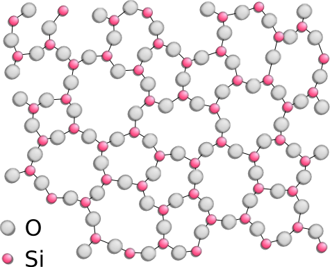
We can use qusecs DR-plans to design materials such as disordered graphene and silica bi-layers [31] [32]. We investigate a more specific problem in a somewhat more general setting: the problem of finding boundary conditions (additional constraints) to add to an underconstrained monolayer to make it isostatic. This can be done in a number of ways: (1) pin together 2 underconstrained monolayers in such a way that the resulting bi-layer becomes isostatic (see Figure 7); (2) pin the boundary of (or in general, add constraints to) a layer (possibly a genus 0 monolayer) so that it becomes isostatic; or (3) design a broader class of structures to ensure they are isostatic, self-similar (via some subdivision rule) and in addition isostatic at each level of the subdivision (see Figure 8).
In all cases, we are specifically interested in how to add additional constraints such that the resulting isostatic structure has a small DR-plan; this way a realization can be found, allowing efficient stress, flex and other property design related to the rigidity matrix. To answer these questions, we first introduce the qusecs’ that are used to model these materials. In this section, we discuss Item (2) in detail.

5.1 Body-Hyperpin Qusecs
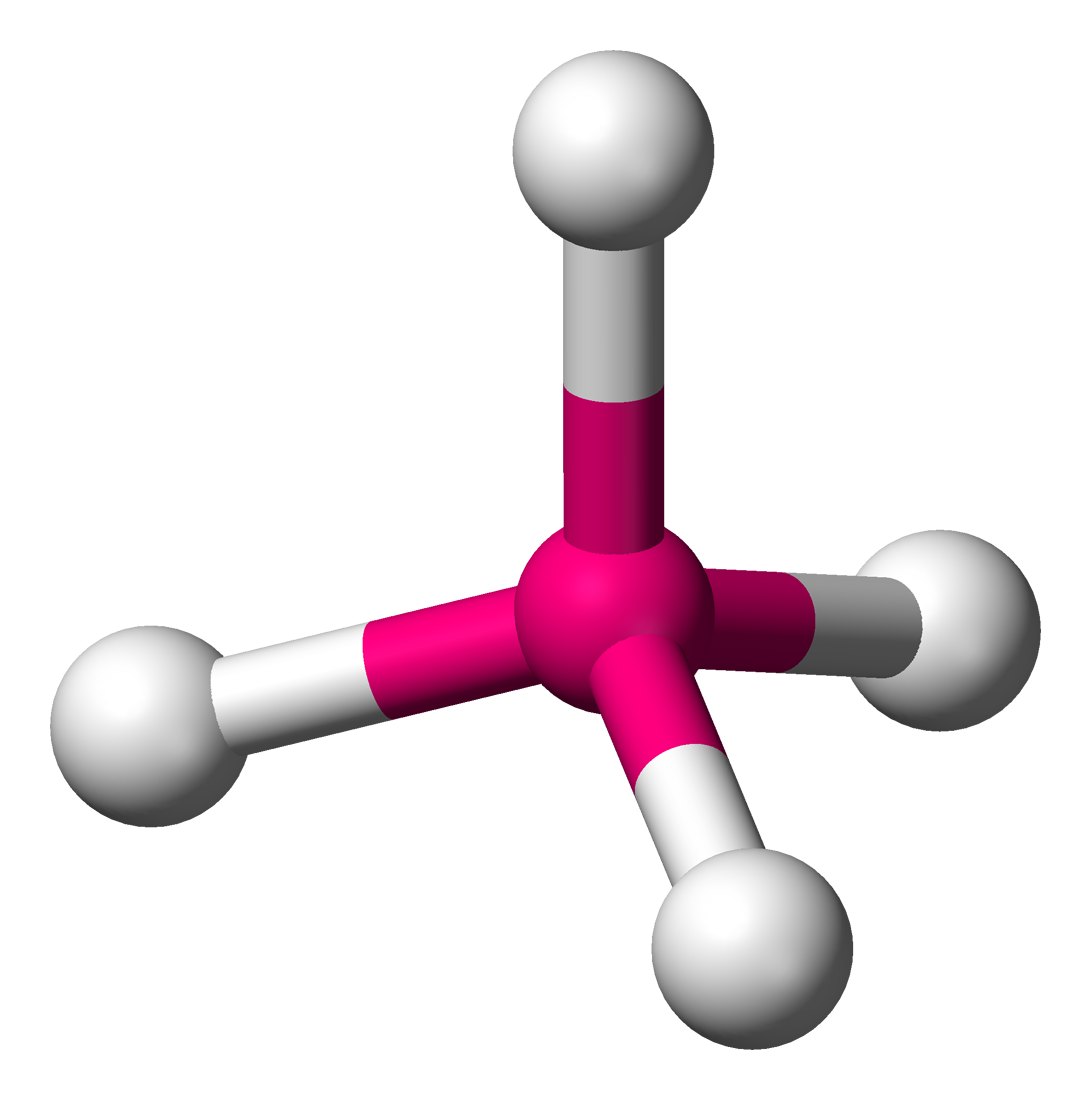
Definition 15.
A body-hyperpin qusecs is a constraint system where the objects are rigid bodies, subsets of which are pinned together by pins; i.e, are incident at a common point.
Remark* 16.
For the remainder of this section, we deal only with the DR-plan of such qusecs. Hence, we refer only to the combinatorics or underlying hypergraph of the qusecs. We now introduce 2 sub-classes of body-hyperpin graphs for modeling Examples 4 and 5 in Section 1, for which the optimal completion problem is significantly easier.
Definition 17.
A body-pin graph is a body-hyperpin graph with the following conditions: (1) each pin is shared by at most two bodies; and (2) no two bodies share more than one pin
Such a body-pin graph, , can also be seen as a body-bar graph, , where the bodies of are the original bodies of and each pin between bodies in are replaced with 2 bars in between the same bodies. Such body-bar graphs with 1 and 2-dof can be characterized by being and -tight respectively [43] [5] (defined in 2.1). See Figure 9(b).
Definition 18.
A triangle-hyperpin graph is a body-hyperpin graph where each body is a triangle, i.e., it shares pins with at most 3 other bodies. This is also represented as a hyper-graph where each pin is a vertex and each triangle represents a tri-hyperedge. For such hypergraphs, 1 and 2-dof can be characterized by and -tightness respectively [43] [5].
Body-pin graphs are of particular interest to us in the context of Example 4 in Section 1. Triangle-multipin graphs can be used to represent the silica bi-layers and glassy structures described in Example 5 of Section 1, where each triangle is the junction of “disks” in the plane (see Figure 7). Typically, these systems are not isostatic, so to relate the work of this paper to the systems, we define a slightly different kind of DR-plan using the notion of -sparsity and tightness.
Definition 19.
A -tight DR-plan is one in which each child node is either a vertex maximal proper -tight sub-graph of the parent node or it is trivial. In our case, the trivial nodes are the bodies.
Provided such -sparse graphs are matroidal (conditions given in [43]), the notion of a canonical DR-plan extends directly to the case when the hypergraph is -sparse (i.e., independent) using the straightforward notion of trivial and non-trivial intersections and -tightness conditions as in Section 3. In particular, we define canonical DR-plans with similar properties for the 1 and 2-dof body-pin and triangle-hyperpin systems defined above.
Observation* 20.
For the 1-dof body-pin graphs described above that are -sparse, a -tight canonical DR-plan exists where every node of a -sparse graph satisfies one of the following: (1) its children are 2 proper vertex-maximal 1-dof graphs that intersect on another 1-dof graph; or (2) its children are all of the proper maximal 1-dof sub-graphs, pairwise sharing at most one body.
As in Section 3, a strong Church-Rosser property holds, making all canonical DR-plans optimal:
Observation* 21.
When the input is independent, all -tight canonical DR-plans are optimal. We can find such a DR-plan in the same time complexity as the -tight case for bar-joint graphs discussed in Section 3.
The above-mentioned algorithm exists because such -tight graphs are matroidal and have a pebble game [43].


The above discussion leads to the main theorem:
Theorem* 22.
Given a 1-dof body-pin or triangle-multipin graph and corresponding 1-dof DR-plan, there is a quadratic algorithm for the 1-dof optimal completion problem of Section 4.
Observation* 23.
Remark 24.
While the proof for Theorem 22 gives us a DR-plan for the isostatic completion with minimum fan-in, (a reasonable measure of algebraic complexity), a more nuanced measure that treats solutions of 1-dof and 2-dof systems as 1 or 2 parameter families would no longer be optimized by the algorithm given in that proof. In particular, the complexity of the standard algorithm in the -dof case would be exponential in (even if the case were matroidal and an optimal DR-plan is known).
6 Application: Finding Optimal DR-Plans and Realizations for Cross-Linking Microfibrils
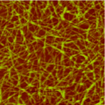
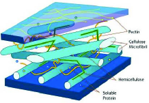
The canonical DR-plan of Section 3 can additionally be applied to analyze and solve the structure of cross-linking collagen microfibrils in animals, cellulose microfibrils in plant cell walls, and actin filaments in the cytoskeleton by modeling these structures as a third type of qusecs, pinned line-incidence systems.
Collagen is an important protein material in biological tissues with highly elastic mechanical properties [60]. Cellulose is the most important constituent of the cell wall of plants (see Figure 10(a)) [61, 62]. Both of these substances consist of a large number microfibrils, each of which is cross-linked at 2 places with usually 3 other fibrils, where the cross-linking is like an incidence constraint that the crosslinked fibrils can slide against each other while remaining incident (see Figure 10(b)).
6.1 Modeling the Fibrils as a Pinned Line-Incidence System
The cross-linking microfibrils can be modeled as a pinned line-incidence constraint system in , where incidence constraints are used instead of distance constraints.
A pinned line-incidence system is a graph together with parameters specifying pins with fixed positions in , such that each edge is constrained to lie on a line passing through the corresponding pin, i.e. . A pinned line-incidence graph is rigid if and for every induced subgraph [36]. Note that no trivial motion exists since the pins have fixed positions on the plane. Euclidean transformations are not factored out. In particular, both a single vertex and a single edge are underconstrained graphs.
In the case of microfibril cross-linking, each fibril is attached to some fixed larger organelle/membrane at one site. Consequently, each fibril can be modeled as an edge of the graph, with the attachment being the corresponding pin. The two cross-linkings in which the fibril participates are modeled as the two vertices in defining the edge.
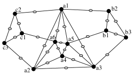
Figure 10(c) shows an example of a pinned line-incidence graph, where the grey ovals denote pins representing attachments of fibrils, and the vertices represent cross-linkings. The graph is isostatic, with 12 vertices and 24 edges/pins.
6.2 Optimal DR-Plan for Pinned Line-Incidence Systems
In this section, we will adapt the results in Section 3 to give the canonical DR-plan for pinned line-incidence graphs. First, we note that an isostatic pinned line-incidence graph can be disconnected, being the disjoint union of two or more isostatic subgraphs. This is because the pins have fixed positions on the plane. We define a trivial graph to be a single vertex and make the following modification to the definition of the canonical DR-plan:
Definition 25.
The DR-plan of a pinned line-incidence graph is one in which (1) each child node of a non-leaf node is either a connected rigid vertex-induced subgraph of , or an edge not contained in any proper rigid subgraph of , and (2) a leaf node is a single edge.
The canonical DR-plan of is one in which the child rigid subgraphs are connected, isostatic vertex-maximal subgraphs of the parent.
Theorem 4 holds for pinned line-incidence graphs with this modified definition. The proof is similar to the original proof (in Section 3) using the same set of lemmas and the following modified version of Observation 5, which can be proved using a simple counting based argument.
Observation 26.
Let and to be subgraphs of the same isostatic graph , where each of them can be either a single edge or a connected isostatic subgraph. There are only two possible cases: (1) at least one of , is an edge, if and only if is underconstrained, if and only if is trivial; and (2) both and are isostatic, if and only if is isostatic, if and only if is isostatic.
Given Observation 26, Lemma 6, Point 1 and 3, straightforwardly extend to pinned line-incidence graphs. The proof of Point 2 for pinned line-incidence graphs is given in A.4.1. Thus it is straightforward to adapt the proof of Theorem 4 to pinned line-incidence graphs. Consequently, we can efficiently find the optimal DR-plan for pinned line-incidence graphs using basically the same algorithm as for bar-joint graphs.
Note: The recombination problem for pinned line-incidence systems is trivial. Since the pins are given fixed positions in the plane, the solutions of a isostatic sub-system will automatically be consistent with solutions of the remaining of the system.
7 Conclusion
We have clarified the main source of complexity for the optimal DR-plan and recombination problems. For the former problem, when there are no overconstraints (as is the case for 2D qusecs whose realizations are many common types of layered materials), we defined a canonical DR-plan and showed that any canonical DR-plan is guaranteed to be optimal, a strong Church-Rosser property. This gives an efficient () algorithm to find an optimal DR-plan that satisfies other desirable characteristics.
We have also described a novel method of efficiently realizing a 2D qusecs from the optimal DR-plan by modifying the otherwise indecomposable systems at nodes of a DR-plan. These results rely on a recent theory of convex Cayley configuration spaces. Relationships and reductions between these and previously studied problems were formally clarified.
We then modeled specific layered materials using extensions of the above theoretical results including the motivating Examples 1-5 in the introduction.
7.1 Open Problems
The first set of problems are from Section 3:
Open Problem 1.
Is there a more efficient algorithm than to find the canonical DR-plan of isostatic 2D bar-joint graphs?
Conjecture 27.
The Modified Frontier Algorithm (MFA) [8] finds a canonical, and hence optimal, DR-plan.
The difficulty of proving Conjecture 27 arises from the fact that MFA, although running in time , is a bottom-up algorithm, involving complex datastructures. However, a proof of optimality, even if it exists, would not be possible without the new notion of a canonical DR-plan at hand. The intuition for this conjecture comes from the similarity of the DR-plan generated by MFA to that of the sequential decomposition described in the proof of Theorem 9. Since it is known [8] that the DR-plan generated by MFA is cluster-minimal, an alternate conjecture is the following.
Conjecture 28.
For independent graphs, cluster-minimal DR-plans are optimal. In fact, for independent graphs, cluster-minimality and canonical are equivalent properties of a DR-plan.
Open Problem 2.
Although generic rigidity is a property of graphs, and moreover, in the case of qusecs, generic rigidity has a combinatorial sparsity and tightness-based characterization, the original definition of independence in the rigidity matroid requires an algebraic notion of independence of vectors of indeterminates over . Thus the definition of the DR-plan requires algebra over the reals. In fact, the recursive decomposition problem is not tied to geometric constraint graphs or an algebraic-geometric or mechanical notion of rigidity, and can be defined for any graph using the notion of an abstract rigidity matroid [63]. This is a type of matroid with two additional matroid axioms; abstract rigidity matroids can be defined in a purely graph-theoretic manner, with no need for algebra in their definition. However, such abstract rigidity need not have a sparsity characterization. On the other hand, there are sparsity matroids that do not correspond to any notion of abstract rigidity. However, when an abstract rigidity matroid is also a sparsity matroid, then the techniques of this paper directly apply and we can obtain purely combinatorially defined recursive decompositions of graphs.
A few natural open questions concern the following common theme that runs through the optimal recombination and later sections of the paper:
Open Problem 3.
For fixed , we have polynomial time optimal DR-planning (Section 3), recombination (modification) in the presence of overconstraints, optimal modification for decomposition OMD when at most constraints are removed (Section 4), and also optimal completion using at most constraints in the body-pin and triangle-multipin cases for a somewhat different optimization of the DR-plan (Section 4.5). However, in the running time of all of these algorithms, appears in the exponent. Can be removed from the exponent?
One problem in the above theme is from Section 5.
Open Problem 4.
What is the complexity of the optimal completion problem when the given graph has more than 2-dofs? Our proof for the 1 and 2-dof cases relied heavily on the matroidal properties of their corresponding -tightness. For higher number of dofs, the characterization is no longer matroidal [43]. As a result, the major obstacle is that there is no easy way of obtaining an optimal or canonical -dof DR-plan in general. Even assuming such a DR-plan is available, if higher dofs had the same characteristics, Observation 24 raises questions about the correct measure of DR-plan size that captures algebraic complexity for recombining graphs with many dofs (this is not an issue in the isostatic case). Unless some restrictions can be found and taken advantage of, the -dof optimal completion problem would have complexity exponential in .
Another problem from the above theme is from Section 4
Open Problem 5.
What is the complexity of the restricted OMD (optimal modification for decomposition) problem? This has the potential to be difficult. For example, when the isostatic completion is required to be a 2-tree the restricted OMD problem is reducible to the maximum spanning series-parallel subgraph problem shown by [64] to be NP-complete even if the input graph is planar of maximum degree at most 6. However, since the OMD problem has other input restrictions such as not having any proper isostatic subgraphs, it is not clear if the reverse reduction exists and hence it is unclear whether the OMD problem is NP-complete.
The same holds for the restricted OMD problem where the isostatic completion is required to be a tree-decomposable graph of low Cayley complexity (i.e. have special, small DR-plans). One potential obstacle to an indecomposable graph ’s membership in the restricted OMDk for small is if is tri-connected and has large girth. In fact, 6-connected (hence rigid) graphs with arbitrarily large girth have been constructed in [65].
Open Problem 6.
Is the OMD (optimal modification for decomposition) problem reducible to the OC (optimal completion) problem?
More general problem directions are the following.
Open Problem 7.
Combinatorial rigidity for periodic structures is an active area of research. This paper motivates a study of the rigidity of self-similar structures, with self-similar groups replacing periodic groups.
Open Problem 8.
The pinned line incidence structures of Section 6, for example in the case of collagen microfibrils, whose function is elastic contraction, should be considered congruent under projective transformations. I.e. the projective group should be factored out as a trivial motion in a new project for extending the combinatorial rigidity characterization of such systems. (Currently we permit no trivial motions at all).
Open Problem 9.
Experimental validation (either computationally or physical experiments) of predications based on the material model and theory used in this paper. This can be done by modeling known materials and putting stresses on them, seeing if the prediction is observed in the real material. Or, our theory could be used to design new materials, which can be tested to see if they possess predicted properties.
Appendix A Proofs
A.1 Proofs from Section 3
A.1.1 Proof of Observation 5
Proof.
For (1), simply note that if were trivial, then, by definition, and must be trivial.
For the next parts, we use the quantity , which we call density. For (2), observe that underconstrained subgraphs of isostatic graphs must have density less than 3. For (3), observe that, given an isostatic graph, a subgraph with density must also be isostatic. Then, use the fact that, by definition, and . Then it is straightforward application of the inclusion-exclusion .
For (4), because subgraphs of a isostatic graph can only be trivial, underconstrained, or isostatic, all cases have already been exhausted. ∎
A.1.2 Proof of Lemma 6, Point 1
Proof.
Assume . This would contradict the proper vertex-maximality of . In the reverse direction, we know is either a non-leaf node (isostatic by definition of a DR-plan) or itself (isostatic by definition of the problem). Thus, is isostatic. ∎
A.1.3 Proof of Lemma 6, Point 2
Observation 29.
Take and . If is isostatic, then there can be no edges in between the vertices of and .
Proof.
Take , , and (note that , and ). Furthermore, take the proper subgraphs , , and that are non-empty.
Assume that there is a third isostatic vertex-maximal proper subgraph (with ). There are possible cases for what this subgraph could be.
Without loss of generality, all graphs are the induced subgraphs of .
-
1.
3 cases: cannot be , , or . This is by definition.
-
2.
13 cases: cannot be a proper subgraph of and or else would not be vertex-maximal. These are the graphs , , , , , , , , , , , , and .
-
3.
2 cases: cannot contain or as proper subgraphs, or else they are not vertex-maximal. These are the graphs and respectively.
-
4.
4 cases: cannot be , , , or because these are all disconnected (Observation 29) and cannot be isostatic.
-
5.
1 case: is not possible. Since we have from Lemma 6, point 1, that cannot be isostatic. We also know it cannot be trivial because it contains isostatic subgraphs. This means it must be underconstrained. From Observation 5, we know that must then be trivial. This is impossible because is isostatic, thereby contradicting the assumption that is isostatic.
-
6.
1 case: is not possible. Since (and ), we know by the same logic as the previous case that the must be trivial (a single node). However, . This causes a contradiction, the intersection cannot be trivial because and are not empty sets and are disjoint.
-
7.
2 cases: and are not possible. The proof mirrors the previous case, except here you must choose and respectively.
-
8.
1 case: is all that remains.
Since it means that , thus proving the Lemma. ∎
A.1.4 Proof of Lemma 6, Point 3
A.2 Proofs from Section 4
A.2.1 Proof of Theorem 12
Proof.
The Cartesian realization space of is computed easily with a DR-plan of size 2, and is the union of solutions (modulo orientation preserving isometries) each with a distinct orientation type, where is the number of triangles in the 2-tree ; here is the restriction of the length vector to the edges in . A desired solution (or connected component of a solution space) of of an orientation type can be found by a subdivided binary search of the Cartesian realization space of of orientation type , as ranges over the discretized convex polytope with bounding hyperplanes described in Theorem 10. A solution is found when the lengths for nonedges in match . ∎
A.3 Proofs from Section 5
A.3.1 Proof of Remark 16
Proof.
We can replace each body that has only one pin by a single vertex. A body with 2 pins can be replaced by an edge. In general, a body with pins can be replaced by a 2-tree on vertices. When finding a DR-plan, we treat each body as trivial, so they become the leaves of the DR-plan. The optimal recombination problem and approach of Section 4 are unchanged. The optimal completion via the optimal modification problem in Section 4 now has an additional restriction that all edges in the 2-tree representation of the bodies must be removed together, not individually. ∎
A.3.2 Proof of Observation 20
Proof.
The existence of this canonical DR-plan follows from the same arguments as in the proof of Theorem 4. The only difference is the definition of a trivial intersection. In this case, when two subgraphs share more than 1 body, they become rigid (in fact over constrained). Sharing a pin is not considered an intersection. Such a structure is viewed as two subgraphs each sharing 1 body with a third 1-dof subgraph which essentially just consists of those two bodies pinned together. ∎
A.3.3 Proof of Theorem 22
Proof.
Suppose we are given a body-pin graph and its corresponding body-bar graph and have obtained the 1-dof DR-plan . Each node of is then a vertex-maximal proper 1-dof subgraph of .
To make the graph isostatic, we need only add one body and pin it to 2 other bodies. Doing so will cause to become -tight.
We adopt the following algorithm. Choose the 2 bodies to pin to by choosing a node in and looking at its children. From Observation 21, we know that the children can only share a single pin or a sub-graph. Pin the new body to bodies in two separate children. Doing so will ensure that all children of will have 1-dof and all ancestors of (including ) will now be isostatic.
Such a pinning covers all possible ways of adding a new body. Assume a new body is added to the input graph and pin it to and to make it isostatic. Then, there is a lowest 1-dof node in such that and appear in . Thus, pinning in the manner described yields an equivalent isostatic DR-plan to pinning to and .
For each node , assign a size of the denoted . . We are looking for that minimizes . Denote the sub-tree of rooted at by and the number of leaves in a tree by . Note that because no descendant of is isostatic. Similarly, for any ancestor of , , where is the child leading to . All other nodes are not isostatic and hence do not appear in the isostatic DR-plan.
The node to be pinned is always the the deepest nontrivial node of some path in . Suppose a node is pinned that has a nontrivial child . Then, , where is essentially the number of leaves between and . If we had instead chosen to pin , then . And for each ancestor of , is unchanged, meaning . Thus we only have to check the deepest non-trivial nodes.
Running the above algorithm brute force gives running time quadratic in the number of bodies of the given body-pin system.
For the multi-triangle pin graphs, we can do the same thing, except we need to add a single triangle to one of the nodes to cause it to become isostatic. ∎
A.3.4 Proof of Observation 23
Proof.
The only difference from the 1-dof case is that now we need to remove 2-dofs from our graph. Start with a 2-dof DR-plan . Like in the previous proof, we need to add a body and 2 pins to 2 nodes to obtain an isostatic DR-plan.
Suppose we pin 2 distinct nodes and . Then, there must exist a common ancestor of and . Then, in , . However, if we chose to pin one of and twice, then . Thus . All ancestors of are unchanged. So .
Thus the only choice is to pin a single node twice. Hence, we can run the same algorithm as the 1-dof case and simply pin twice instead of once. ∎
A.3.5 Proof of Observation 24
Proof.
An isostatic graph has 3 parameters that define its position and orientation. These are the Euclidean motions. A 1-dof graph has 4 parameters: the 3 Euclidean motions and a dof parameter. A 2-dof has 5 parameters. The number of parameters roughly correlates with the algebraic complexity of obtaining a realization.
Thus, starting with a as described in the proof for Remark 22, when a node is pinned, the same structure is preserved as before. Suppose is an isostatic node after pinning . Then, the children of (except one if ) have 1-dof. The realization complexity for is simply that of realizing each of its children. In general, the number of parameters for will be , if and , where is the number of -dof children of .
Minimizing the algebraic complexity requires minimizing the maximum for any node . In this case, it is not possible to always choose to pin a node closest to a leaf in the tree, because it could have high fan-in. So we try brute force by pinning all nodes to pick the one with the lowest algebraic complexity. This algorithm is still quadratic for the 1-dof case.
For the 2-dof situation, there are more cases to consider. If we pin the same node twice as above, we have for any ancestor and . If we pin a node and one of its ancestors , then any nodes between and will be 1-dof, any nodes above will be isostatic, and nodes below will be 2-dof. Note that solving or realizing will also realize . Next, we need to consider nodes above and including in our complexity: and for an ancestor of .
The only remaining case is pinning two nodes that are incomparable, i.e. do not have a descendant/ancestor relationship. The only change from the previous case is that for the lowest common ancestor of the nodes , . For any ancestor of , we still have .
Like the 1-dof case, we again cannot simply choose the nodes deepest in the tree to pin. However, neither can we assume pinning one node twice will give us the best algebraic complexity. Hence, we will need to check each pair of nodes to pin. This makes our brute-force algorithm , where is the number of bodies. ∎
A.4 Proofs from Section 6
A.4.1 Proof of Lemma 6, Point 2 — for 2-dimensional pinned line incidence graphs
Proof.
We use the same notation as in the original proof of Lemma 6, Point 2, given above. Without loss of generality, all graphs are the induced graphs on .
First notice that since is isostatic, by Observation 26, both and are connected isostatic vertex-maximal proper subgraphs of . Since , there are no edges in that is not contained in a isostatic subgraph, so does not have any single-edge child node, and is a connected isostatic vertex-maximal proper subgraph of .
We analyze all the possible cases for .
- 1.
-
2.
1 case: is not possible. The proof is similar to the previous case.
-
3.
2 cases: and are not possible. The proof is similar to the previous case.
All remaining cases are similar to the original proof for 2D bar-joint graphs. ∎
References
- [1] M. Sitharam, Combinatorial approaches to geometric constraint solving: Problems, progress, and directions, In: DIMACS: Series in Discrete Mathematics and Theoretical Computer Science 67 (2005) 117.
- [2] C. M. Hoffman, A. Lomonosov, M. Sitharam, Decomposition plans for geometric constraint systems, part i: Performance measures for cad, Journal of Symbolic Computation 31 (4) (2001) 367–408. doi:10.1006/jsco.2000.0402.
- [3] C. M. Hoffman, A. Lomonosov, M. Sitharam, Decomposition plans for geometric constraint problems, part ii: new algorithms, Journal of Symbolic Computation 31 (4) (2001) 409–427. doi:10.1006/jsco.2000.0403.
-
[4]
G. Laman, On graphs and rigidity of
plane skeletal structures, Journal of Engineering Mathematics 4 (1970)
331–340, 10.1007/BF01534980.
URL http://dx.doi.org/10.1007/BF01534980 - [5] I. Streinu, L. Theran, Sparse hypergraphs and pebble game algorithms, European Journal of Combinatorics 30 (8) (2009) 1944–1964. doi:10.1016/j.ejc.2008.12.018.
- [6] T.-S. Tay, Rigidity problems in bar and joint frameworks, Ph.D. thesis, University of Waterloo (1976).
- [7] N. White, W. Whiteley, The algebraic geometry of motions of bar-and-body frameworks, SIAM Journal on Algebraic Discrete Methods 8 (1) (1987) 1–32.
- [8] A. Lomonosov, Graph and combinatorial analysis for geometric constraint graphs, Ph.D. thesis, University of Florida (2004).
- [9] M. Sitharam, J. Peters, Y. Zhou, Optimized parametrization of systems of incidences between rigid bodies, Journal of Symbolic Computation 45 (4) (2010) 481–498.
- [10] M. Sitharam, Well-formed systems of point incidences for resolving collections of rigid bodies, International Journal of Computational Geometry & Applications 16 (05n06) (2006) 591–615.
- [11] M. Sitharam, Y. Zhou, J. Peters, Reconciling conflicting combinatorial preprocessors for geometric constraint systems, International Journal of Computational Geometry & Applications 20 (06) (2010) 631–651.
- [12] M. Sitharam, H. Gao, Characterizing graphs with convex and connected configuration spaces, Discrete & Computational Geometry 43 (3) (2010) 594–625. doi:10.1007/s00454-009-9160-8.
-
[13]
M. Sitharam, M. Wang, H. Gao, Cayley configuration spaces of 2d mechanisms
part i: extreme points, continuous motion paths and minimal representations, Under review. arXiv preprint arXiv:1112.6008 (2011). arXiv:1112.6008. -
[14]
M. Sitharam, M. Wang, H. Gao, Cayley configuration spaces of 2d mechanisms
part ii: combinatorial characterization, Under review. arXiv preprint arXiv:1112.6009 (2011). arXiv:1112.6009. - [15] M. Sitharam, M. Wang, How the beast really moves: Cayley analysis of mechanism realization spaces using caymos, Computer-Aided Design 46 (0) (2014) 205 – 210, 2013 SIAM Conference on Geometric and Physical Modeling.
- [16] M. Sitharam, M. Wang, Cayley configuration space analysis by CayMos: software architecture and functionalities, In preparation.
- [17] M. Wang, M. Sitharam, Cayley analysis of mechanism configuration spaces using caymos: Software functionalities and architecture, ACM Transactions on Mathematical Software.
-
[18]
R. Joan-Arinyo, A. Soto-Riera, S. Vila-Marta, J. Vilaplana-Pastó,
Transforming an
under-constrained geometric constraint problem into a well-constrained one,
in: Proceedings of the eighth ACM symposium on Solid modeling and
applications, SM ’03, ACM, New York, NY, USA, 2003, pp. 33–44.
doi:10.1145/781606.781616.
URL http://doi.acm.org/10.1145/781606.781616 - [19] M. E. Gaspar, P. Csermely, Rigidity and flexibility of biological networks, ArXiv e-printsarXiv:1204.6389.
-
[20]
Wikimedia Commons,
Chlamydomonas
tem 17,
https://commons.wikimedia.org/wiki/File:Chlamydomonas_TEM_17.jpg
(2007).
URL https://commons.wikimedia.org/wiki/File:Chlamydomonas_TEM_17.jpg - [21] S. J. Hollister, Bme 332: Introduction to biosolid mechanics, http://www.umich.edu/~bme332/ch10ligten/ligten2.jpg (2007).
-
[22]
Wikimedia Commons,
Rothemund
dna sierpinski gasket,
https://commons.wikimedia.org/wiki/File:Rothemund-DNA-SierpinskiGasket.jpg
(2007).
URL https://commons.wikimedia.org/wiki/File:Rothemund-DNA-SierpinskiGasket.jpg -
[23]
D. J. Needleman, M. A. Ojeda-Lopez, U. Raviv, H. P. Miller, L. Wilson, C. R.
Safinya,
Higher-order
assembly of microtubules by counterions: From hexagonal bundles to living
necklaces, Proceedings of the National Academy of Sciences of the United
States of America 101 (46) (2004) 16099–16103.
arXiv:http://www.pnas.org/content/101/46/16099.full.pdf+html, doi:10.1073/pnas.0406076101.
URL http://www.pnas.org/content/101/46/16099.abstract -
[24]
F. R. Garcia-Gonzalo, J. F. Reiter,
Scoring a backstage
pass: Mechanisms of ciliogenesis and ciliary access, The Journal of Cell
Biology 197 (6) (2012) 697–709.
arXiv:http://jcb.rupress.org/content/197/6/697.full.pdf+html, doi:10.1083/jcb.201111146.
URL http://jcb.rupress.org/content/197/6/697.abstract -
[25]
Wikimedia Commons,
Afm
height image of carboxymethylated nanocellulose adsorbed on a silica
surface.,
https://commons.wikimedia.org/wiki/File:AFM_Innventia_nanocellulose.JPG
(2010).
URL https://commons.wikimedia.org/wiki/File:AFM_Innventia_nanocellulose.JPG -
[26]
Wikimedia Commons,
Plant
cell wall diagram,
https://commons.wikimedia.org/wiki/File:Plant_cell_wall_diagram.svg
(2007).
URL https://commons.wikimedia.org/wiki/File:Plant_cell_wall_diagram.svg -
[27]
T. Björkman, S. Kurasch, O. Lehtinen, J. Kotakoski, O. V. Yazyev,
A. Srivastava, V. Skakalova, J. H. Smet, U. Kaiser, A. V. Krasheninnikov,
Defects in bilayer silica and
graphene: common trends in diverse hexagonal two-dimensional systems,
Scientific Reports 3 (3482).
doi:10.1038/srep03482.
URL http://dx.doi.org/10.1038/srep03482 -
[28]
F. R. Eder, J. Kotakoski, U. Kaiser, J. C. Meyer,
A journey from order to disorder
— Atom by atom transformation from graphene to a 2D carbon glass,
Scientific Reports 4 (4060).
doi:10.1038/srep04060.
URL http://dx.doi.org/10.1038/srep04060 - [29] P. W. K. Rothemund, N. Papadakis, E. Winfree, Algorithmic self-assembly of dna sierpinski triangles, PLoS Biology 2 (12). doi:10.1371/journal.pbio.0020424.
-
[30]
Wikimedia Commons,
Finite
subdivision of a radial link,
https://commons.wikimedia.org/wiki/File:Finite_subdivision_of_a_radial_link.png
(2012).
URL https://commons.wikimedia.org/wiki/File:Finite_subdivision_of_a_radial_link.png - [31] M. Wilson, A. Kumar, D. Sherrington, M. F. Thorpe, Modeling vitreous silica bilayers, Physical Review B 87 (21) (2013) 214108. arXiv:1303.5898, doi:10.1103/PhysRevB.87.214108.
-
[32]
M. Heyde, Structure
and motion of a 2d glass, Science 342 (6155) (2013) 201–202.
arXiv:http://www.sciencemag.org/content/342/6155/201.full.pdf, doi:10.1126/science.1245217.
URL http://www.sciencemag.org/content/342/6155/201.short - [33] A. Donev, S. Torquato, F. H. Stillinger, R. Connelly, Jamming in hard sphere and disk packings, Journal of Applied Physics 95 (3).
-
[34]
X.-S. Gao, Q. Lin, G.-F. Zhang,
A c-tree decomposition
algorithm for 2d and 3d geometric constraint solving, Comput. Aided Des.
38 (1) (2006) 1–13.
doi:10.1016/j.cad.2005.03.002.
URL http://dx.doi.org/10.1016/j.cad.2005.03.002 -
[35]
B. Jackson, T. Jordán,
Pin-collinear body-and-pin
frameworks and the molecular conjecture, Discrete & Computational Geometry
40 (2) (2008) 258–278.
doi:10.1007/s00454-008-9100-z.
URL http://dx.doi.org/10.1007/s00454-008-9100-z - [36] M. Sitharam, M. Tarifi, M. Wang, An incidence geometry approach to dictionary learning, in: Proceedings of CCCG 2014, 2014.
- [37] L. Asimow, B. Roth, The rigidity of graphs, Transactions of the American Mathematical Society 245 (1978) 279–289. doi:http://dx.doi.org/10.1090/S0002-9947-1978-0511410-9.
- [38] L. Lovasz, Y. Yemini, On generic rigidity in the plane, SIAM Journal on Algebraic Discrete Methods 3 (1) (1982) 91–98.
- [39] A. Lee, I. Streinu, L. Theran, Graded sparse graphs and matroids., J. UCS 13 (11) (2007) 1671–1679.
-
[40]
D. J. Jacobs, B. Hendrickson,
An
algorithm for two-dimensional rigidity percolation: The pebble game, Journal
of Computational Physics 137 (2) (1997) 346 – 365.
doi:http://dx.doi.org/10.1006/jcph.1997.5809.
URL http://www.sciencedirect.com/science/article/pii/S0021999197958095 -
[41]
C. M. Hoffmann, A. Lomonosov, M. Sitharam,
Finding solvable subsets of
constraint graphs, in: G. Smolka (Ed.), Principles and Practice of
Constraint Programming-CP97, Vol. 1330 of Lecture Notes in Computer Science,
Springer Berlin Heidelberg, 1997, pp. 463–477.
doi:10.1007/BFb0017460.
URL http://dx.doi.org/10.1007/BFb0017460 - [42] C. Jermann, G. Trombettoni, B. Neveu, P. Mathis, Decomposition of geometric constraint systems: a survey, International Journal of Computational Geometry & Applications 16 (05n06) (2006) 379–414.
- [43] A. Lee, I. Streinu, Pebble Game Algorithms and Sparse Graphs, ArXiv Mathematics e-printsarXiv:math/0702129.
-
[44]
J. C. Owen, Algebraic solution
for geometry from dimensional constraints, in: Proceedings of the First ACM
Symposium on Solid Modeling Foundations and CAD/CAM Applications, SMA ’91,
ACM, New York, NY, USA, 1991, pp. 397–407.
doi:10.1145/112515.112573.
URL http://doi.acm.org/10.1145/112515.112573 -
[45]
I. Fudos, C. M. Hoffmann, A
graph-constructive approach to solving systems of geometric constraints, ACM
Trans. Graph. 16 (2) (1997) 179–216.
doi:10.1145/248210.248223.
URL http://doi.acm.org/10.1145/248210.248223 -
[46]
R. Joan-Arinyo, A. Soto-Riera, S. Vila-Marta, J. Vilaplana-Pastó,
Revisiting
decomposition analysis of geometric constraint graphs, Computer-Aided Design
36 (2) (2004) 123 – 140, solid Modeling and Applications.
doi:http://dx.doi.org/10.1016/S0010-4485(03)00057-5.
URL http://www.sciencedirect.com/science/article/pii/S0010448503000575 - [47] J. Saxe, Embeddability of weighted graphs in k-space is strongly np-hard, in: Proceedings of 17th Allerton Conference in Communications, Control and Computing, 1979, pp. 480–489.
- [48] C. Borcea, I. Streinu, The number of embeddings of minimally rigid graphs, Discrete & Computational Geometry 31 (2) (2004) 287–303. doi:10.1007/s00454-003-2902-0.
-
[49]
M. Sitharam, A. Arbree, Y. Zhou, N. Kohareswaran,
Solution space navigation
for geometric constraint systems, ACM Trans. Graph. 25 (2) (2006) 194–213.
doi:10.1145/1138450.1138452.
URL http://doi.acm.org/10.1145/1138450.1138452 - [50] M. R. Hidalgo, R. Joan-Arinyo, The reachability problem in constructive geometric constraint solving based dynamic geometry, Journal of Automated Reasoning (2011) 1–24.
- [51] Key Curriculum, The geometer’s sketchpad, http://www.keycurriculum.com/ (1995).
- [52] J. M. Porta, L. Ros, O. Bohigas, M. Manubens, C. Rosales, L. Jaillet, An open-source toolbox for motion analysis of closed-chain mechanisms, in: Computational Kinematics, Springer, 2014, pp. 147–154, cUIK.
- [53] Siemens, D-cubed, http://www.plm.automation.siemens.com/en_us/products/open/d-cubed/ (1999).
- [54] P. Todd, Geometry expressions: A constraint based interactive symbolic geometry system, in: Automated Deduction in Geometry, Springer, 2007, pp. 189–202.
- [55] J. Valdes, R. E. Tarjan, E. L. Lawler, The recognition of series parallel digraphs, in: Proceedings of the eleventh annual ACM symposium on Theory of computing, ACM, 1979, pp. 1–12.
- [56] G.-F. Zhang, X.-S. Gao, Well-constrained completion and decomposition for under-constrained geometric constraint problems, International Journal of Computational Geometry & Applications 16 (05n06) (2006) 461–478.
-
[57]
Wikimedia Commons,
Silica,
https://commons.wikimedia.org/wiki/File:Silica.svg (2008).
URL https://commons.wikimedia.org/wiki/File:Silica.svg -
[58]
Wikimedia Commons,
Tetrahedral
3d balls,
https://commons.wikimedia.org/wiki/File:Tetrahedral-3D-balls.png
(2006).
URL https://commons.wikimedia.org/wiki/File:Tetrahedral-3D-balls.png - [59] J. W. Canon, W. J. Floyd, W. R. Parry, Finite subdivision rules, Conform. Geom. Dyn. (2001) 153–196.
- [60] M. J. Buehler, Nanomechanics of collagen fibrils under varying cross-link densities: atomistic and continuum studies, Journal of the mechanical behavior of biomedical materials 1 (1) (2008) 59–67.
- [61] A. B. Fall, S. B. Lindström, J. Sprakel, L. Wågberg, A physical cross-linking process of cellulose nanofibril gels with shear-controlled fibril orientation, Soft Matter 9 (6) (2013) 1852–1863.
- [62] G. Smith, Plant cell wall structure and cell wall growth, Tuatara 19 (1971) 43–50.
-
[63]
J. E. Graver, B. Servatius, H. Servatius,
Combinatorial rigidity, Graduate
studies in mathematics, American mathematical society, Providence (R.I.),
1993.
URL http://opac.inria.fr/record=b1131810 -
[64]
L. Cai, F. Maffray,
On
the {SPANNING} k-tree problem, Discrete Applied Mathematics 44 (1-3)
(1993) 139 – 156.
doi:http://dx.doi.org/10.1016/0166-218X(93)90228-G.
URL http://www.sciencedirect.com/science/article/pii/0166218X9390228G - [65] B. Servatius, On the rigidity of ramanujan graphs, Ann. Univ. Sci. Budapest. Eötvös Sect. Math 43 (2000) 165–170.