Multilevel Quasi-Monte Carlo Methods for Lognormal Diffusion Problems

Abstract

In this paper we present a rigorous cost and error analysis of a multilevel estimator based on randomly shifted Quasi-Monte Carlo (QMC) lattice rules for lognormal diffusion problems. These problems are motivated by uncertainty quantification problems in subsurface flow. We extend the convergence analysis in [Graham et al., Numer. Math. 2014] to multilevel Quasi-Monte Carlo finite element discretizations and give a constructive proof of the dimension-independent convergence of the QMC rules. More precisely, we provide suitable parameters for the construction of such rules that yield the required variance reduction for the multilevel scheme to achieve an $\varepsilon$-error with a cost of $\mathcal{O}(\varepsilon^{-\theta})$ with $\theta<2$, and in practice even $\theta\approx 1$, for sufficiently fast decaying covariance kernels of the underlying Gaussian random field inputs. This confirms that the computational gains due to the application of multilevel sampling methods and the gains due to the application of QMC methods, both demonstrated in earlier works for the same model problem, are complementary. A series of numerical experiments confirms these gains. The results show that in practice the multilevel QMC method consistently outperforms both the multilevel MC method and the single-level variants even for non-smooth problems.

1 Introduction

This paper gives a rigorous error analysis, together with numerical experiments, for a multilevel Quasi-Monte Carlo scheme applied to linear functionals of the solution of a typical model elliptic problem of steady-state flow in random porous media. This problem is of central importance in the development of efficient uncertainty quantification tools for subsurface flow problems. The random elliptic partial differential equation (PDE) reads

$$-\nabla\cdot\big{(}a(\vec{x},\omega)\nabla u(\vec{x},\omega)\big{)}\,=\,f(\vec{x}),\qquad\textnormal{for }\ \vec{x}\in D,\;\;\omega\in\Omega\,,$$ (1.1)

where $D$ is a bounded domain in $\mathbb{R}^{d}$ for $d=1,2$ or $3$, and $\Omega$ is the sample space of a probability space $(\Omega,\mathcal{A},P)$, with $\sigma$-algebra $\mathcal{A}$ and probability measure $P$. A key feature is the coefficient $a(\cdot,\omega)$, which is a lognormal random field on the domain $D$.

In the context of flow through a porous medium, $u$ is the hydrostatic pressure, $a$ is the permeability and $\vec{q}:=-a\nabla u$ is the Darcy flux. This empirical relation between pressure and flux is known as Darcy’s law. When complemented by the conservation condition $\nabla\cdot\vec{q}=f$, where $f(\vec{x})$ is a deterministic source term, this leads to (1.1).

In this paper, the uncertain permeability is assumed to take the form

$$a(\vec{x},\omega)\,=\,a_{*}(\vec{x})+a_{0}(\vec{x})\exp\bigg{(}\sum_{j=1}^{\infty}\sqrt{\mu_{j}}\,\xi_{j}(\vec{x})\,Y_{j}(\omega)\bigg{)},\quad\text{ with }Y_{j}\sim\mathcal{N}(0,1)\text{ i.i.d.}\,,$$ (1.2)

where $a_{*}$ and $a_{0}$ are given deterministic functions on $D$, satisfying $a_{*}(\vec{x})\geq 0$ and $a_{0}(\vec{x})>0$. The sequence $\{\mu_{j}\}$ of nonnegative values is assumed to be enumerated in nonincreasing order, accumulating only at zero, and the sequence $\{\xi_{j}\}$ is $L_{2}(D)$-orthonormal. If they correspond to the eigenvalues and eigenfunctions of the covariance operator of a correlated Gaussian random field, then the infinite sum under the bracket in (1.2) is known as the Karhunen-Loève (KL) expansion of this Gaussian random field (see e.g. [27]).

For simplicity, we only study this problem subject to deterministic boundary conditions. In general, we may have mixed Dirichlet/Neumann conditions. Let the boundary $\Gamma=\partial D$ be partitioned into two open, disjoint parts $\Gamma_{\mathcal{D}}$ and $\Gamma_{\mathcal{N}}$, and let $\vec{n}(\vec{x})$ denote the exterior unit normal vector to $D$ at $\vec{x}\in\Gamma_{\mathcal{N}}$. Then we set

$$u(\vec{x},\cdot) \,=\,\phi_{\mathcal{D}}(\vec{x}) \textnormal{for }\ \vec{x}\in\Gamma_{\mathcal{D}}\,,$$ (1.3)

$$\vec{n}(\vec{x})\cdot\big{(}a(\vec{x},\cdot)\nabla u(\vec{x},\cdot)\big{)} \,=\,\phi_{\mathcal{N}}(\vec{x}) \textnormal{for }\ \vec{x}\in\Gamma_{\mathcal{N}}\,.$$ (1.4)

For $d=2,3$, we assume $D$ to be Lipschitz polygonal/polyhedral and each of $\Gamma_{\mathcal{D}}$ and $\Gamma_{\mathcal{N}}$ to consist of the union of a finite number of edges/faces.

Our goal is to obtain statistical information on certain linear functionals $\mathcal{G}$ of the solution $u$ to (1.1); we write $F:=\mathcal{G}(u)$. In particular, we are interested in the expected value $\mathbb{E}[F]=\mathbb{E}[\mathcal{G}(u)]$ (with respect to the probability measure $P$). We need to perform several discretisation/truncation steps to obtain computable approximations to $\mathbb{E}[F]$:

1. For a sample $\omega$, we employ a standard Galerkin finite element (FE) method with continuous, piecewise linear elements to discretise the solution to the PDE (1.1) on a family of simplicial meshes $\mathcal{T}_{h}$ parametrised by their mesh size $h$. We approximate entries of the element stiffness matrices by a one-point Gauss rule, that is, we evaluate the coefficient at the mid point of each mesh element. We denote the FE approximation on $\mathcal{T}_{h}$ by $u_{h}$.

2. We truncate the KL expansion of $\log(a-a_{*})$ in (1.2) after a finite number of $s$ terms; we denote the $s$-term truncated diffusion coefficient by $a_{s}$ and the corresponding PDE solution by $u_{s}$. The FE approximation to (1.1) on $\mathcal{T}_{h}$ with $a$ replaced by $a_{s}$ then reduces to a function $u_{h,s}$ of $s$ i.i.d. standard Gaussian random variables $Y_{j}$, $j=1,\dots,s$. Denoting the approximation of $F$ by $F_{h,s}:=\mathcal{G}(u_{h,s})$, the expected value $\mathbb{E}[F]$ is then approximated by

   $$\mathbb{E}[F_{h,s}]\,=\,\int_{\mathbb{R}^{s}}\mathcal{G}(u_{h,s}(\cdot,{\boldsymbol{y}}))\prod_{j=1}^{s}\phi(y_{j})\,\mathrm{d}{\boldsymbol{y}}\,,$$ (1.5)

   where $\phi(y)$ denotes the standard Gaussian probability density function. In porous media flow applications, the truncation dimension $s$ is often very large.

3. The $s$-dimensional Gaussian integral in (1.5) is then approximated by an $N$-point quadrature rule, for example a Monte Carlo, sparse grid or Quasi-Monte Carlo rule, or by a multilevel variant (see below).

In this paper the quadrature rules are derived from suitable Quasi-Monte Carlo (QMC) rules (i.e. equal weight rules on the $s$-dimensional unit cube), as we explain in the next section. The single-level variants of these rules, as estimators for (1.5), were analysed for the same model problem in the paper [13] (see also the earlier paper [23] for the uniform case). Much emphasis was placed there on the design of QMC rules that achieve dimension-independent error bounds with good convergence rates and under weak assumptions.

Multilevel methods were introduced by [18, 11]. In the present context multilevel Monte Carlo (MLMC) estimators for (1.5) (multilevel methods based on Monte Carlo integration) have attracted attention because of their capacity to reduce the cost without loss of accuracy. The idea of using such multilevel estimators for the approximation of $\mathbb{E}[F]$ was established in [2, 6] and, for the lognormal case, analysed subsequently in [5, 34].

The multilevel method is based on a sequence of ${L+1}$ FE approximations of increasing accuracy as $\ell$ runs from $0$ to $L$, with mesh diameters $h_{\ell}$ satisfying $h_{0}>h_{1}>\ldots>h_{L}$. At level $\ell$ we also truncate the KL expansion after $s_{\ell}$ terms, with $s_{0}\leq s_{1}\leq\cdots\leq s_{L}$. With the level $\ell$ approximation of our output functional $F$ denoted by $F_{\ell}:=F_{h_{\ell},s_{\ell}}$, we can write $F_{L}$ as the telescoping sum

$$F_{L}\,=\,F_{0}+\sum_{\ell=1}^{L}(F_{\ell}-F_{\ell-1})\,.$$ (1.6)

Then by linearity of the expectation operator we have

$$\mathbb{E}[F_{L}]\,=\,\mathbb{E}[F_{0}]+\sum_{\ell=1}^{L}\mathbb{E}[F_{\ell}-F_{\ell-1}]\,.$$ (1.7)

In the MLMC scheme each term is approximated by an independent Monte Carlo calculation, with a resulting gain in efficiency arising from the fact that the differences $F_{\ell}-F_{\ell-1}$ on the higher levels, although more expensive to compute, have smaller variance and so require fewer Monte Carlo samples.

In this paper, each of the $L+1$ terms in (1.7) is instead approximated by a different QMC rule, where the number of quadrature points can again be chosen to decrease with $\ell$. For sufficiently smooth integrands, QMC quadrature rules offer the prospect of a higher accuracy for the same computational cost compared to standard Monte Carlo quadrature, or a lower cost for the same accuracy. Hence, the goal of this paper is to explore the combination of multilevel estimators and QMC methods by constructing and analysing a multilevel Quasi-Monte Carlo (MLQMC) estimator for the approximation of (1.5). It was first observed in the context of stochastic differential equations in [12] that the two gains can be complementary.

In the context of (1.1), single- and multi-level QMC FE approximations were analysed also in the recent papers [24, 9], but for the simpler case of uniform and affine parameter dependence: in those papers the random variables $Y_{j}$ appeared linearly in the differential operator, and their values were assumed to be uniformly distributed on a bounded interval. The lognormal case considered here is technically more involved and the error bounds for the QMC rules developed here differ essentially from those for the uniform case. They require, for example, so-called “mixed regularity” of the solution of (1.5). As shown here, this mandates stronger assumptions on the data than those required for MLMC or single-level QMC. The importance of this mixed regularity has already been recognised in [16]. In the present paper, we establish for the first time $s$-independent quadrature error bounds for MLQMC estimators and present detailed numerical experiments indicating that MLQMC methods can outperform single-level QMC and MLMC methods in terms of accuracy versus computational cost. Some numerical experiments have also been reported in [30].

The structure of this paper is as follows. Section 2 explains the mechanics of QMC methods, without entering into the question of approximation quality. Section 3 introduces the multilevel QMC method (MLQMC), establishes an abstract convergence theorem, compares the complexity of MLQMC to other estimators, and discusses practical aspects and a practical implementation. Section 4 presents numerical results which confirm the theoretical results. All technical parts related to the necessary QMC convergence and construction theory are relegated to Section 5.

2 Quasi-Monte Carlo Quadrature

Quasi-Monte Carlo quadrature rules are equal weight quadrature rules for integrals over the $s$-dimensional unit cube $[0,1]^{s}$. For this reason we introduce a change of variables ${\boldsymbol{y}}=\boldsymbol{\Phi}_{s}^{-1}({\boldsymbol{\zeta}})$, where $\boldsymbol{\Phi}_{s}^{-1}({\boldsymbol{\zeta}}):=[\Phi^{-1}(\zeta_{1}),\Phi^{-1}(\zeta_{2}),\ldots,\Phi^{-1}(\zeta_{s})]^{\tt T}$ denotes the inverse cumulative normal distribution applied to each component of ${\boldsymbol{\zeta}}\in[0,1]^{s}$. We then obtain from (1.5) the expression

$$\mathbb{E}[F_{h,s}]\,=\,\int_{[0,1]^{s}}F_{h,s}(\boldsymbol{\Phi}_{s}^{-1}({\boldsymbol{\zeta}}))\,\mathrm{d}{\boldsymbol{\zeta}}\,.$$ (2.1)

For the approximation of $\mathbb{E}[F_{h,s}]$ in a single-level scheme, we employ a specific kind of QMC quadrature rule, namely, the shifted rank-$1$ lattice rule given by

$${\mathcal{Q}_{s,N}(F_{h,s};{\boldsymbol{\Delta}})}\,:=\,\frac{1}{N}\sum_{i=1}^{N}F_{h,s}\left(\boldsymbol{\Phi}_{s}^{-1}\left(\operatorname*{frac}\left(\frac{i\,{\boldsymbol{z}}}{N}+{\boldsymbol{\Delta}}\right)\right)\right)\,,\quad i=1,\dots,N\,,$$ (2.2)

where ${\boldsymbol{z}}\in\mathbb{N}^{s}$ is the associated generating vector and ${\boldsymbol{\Delta}}\in[0,1]^{s}$ is the shift. The symbol $\operatorname*{frac}(\cdot)$ denotes the fractional part function, which is to be applied to every component of the $s$-dimensional input vector. For the general theory and fast construction of QMC lattice rules for the $s$-dimensional cube, see e.g., [20] as well as [29, 7, 10]. For the particular case of integrals defined initially over $\mathbb{R}^{s}$, see e.g., [25, 28].

The purely deterministic estimator (2.2) for $\mathbb{E}[F_{h,s}]$ is biased. To remove this statistical bias we construct the associated randomly shifted lattice rule where the random shift ${\boldsymbol{\Delta}}$ is uniformly distributed over $[0,1]^{s}$. We then use the sample average of $\mathcal{Q}_{s,N}(F_{h,s};{\boldsymbol{\Delta}})$ over a fixed, finite number $R$ of shift realizations as an estimator for $\mathbb{E}[F_{h,s}]$. We arrive at

$$\mathcal{Q}_{s,N,R}(F_{h,s})\,:=\,\frac{1}{R}\sum_{k=1}^{R}\mathcal{Q}_{s,N}(F_{h,s};{\boldsymbol{\Delta}}_{k})\,,$$ (2.3)

where $\mathcal{Q}_{s,N}(F_{h,s};{\boldsymbol{\Delta}}_{k})$ is defined in (2.2), $k=1,\dots,R$. Now, let $\mathbb{E}_{\Delta}[\cdot]$ denote the expected value with respect to one or more random shifts. Since

$$\begin{split}\mathbb{E}_{\Delta}[\mathcal{Q}_{s,N}(F_{h,s};\Delta)]&\,=\,\int_{[0,1]^{s}}\frac{1}{N}\sum_{i=1}^{N}F_{h,s}\left(\boldsymbol{\Phi}_{s}^{-1}\left(\text{frac}\left(\frac{i\,{\boldsymbol{z}}}{N}+\Delta\right)\right)\right)\,\mathrm{d}\Delta\\ &\,=\,\frac{1}{N}\sum_{i=1}^{N}\int_{[0,1]^{s}}F_{h,s}(\boldsymbol{\Phi}_{s}^{-1}(\Delta))\,\mathrm{d}\Delta\,=\,\mathbb{E}[F_{h,s}]\,,\end{split}$$

the quantity in (2.3) is an unbiased estimator for $\mathbb{E}[F_{h,s}]$. However, (2.3) is not an unbiased estimator for $\mathbb{E}[F]$, because the error arising from FE approximation and from truncation of the KL expansion of $\log(a-a_{*})$ cannot be removed by randomisation of (2.2). Specifically, the error analysis for randomly shifted lattice rules is carried out in terms of the root mean square error (RMSE)

$$e\big{(}\mathcal{Q}_{s,N,R}(F_{h,s})\big{)}\,:=\,\sqrt{\mathbb{E}_{\Delta}\big{[}\big{(}\mathcal{Q}_{s,N,R}(F_{h,s})-\mathbb{E}[F]\big{)}^{2}\big{]}}\,.$$ (2.4)

Since the random diffusion coefficient $a$ in (1.1) is statistically independent of the random shift in the QMC quadrature rule, it is easy to see that in the single-level scheme we can split the RMSE as follows

$$e\big{(}\mathcal{Q}_{s,N,R}(F_{h,s})\big{)}^{2}\,=\,\mathbb{E}_{\Delta}\big{[}\big{(}\mathcal{Q}_{s,N,R}(F_{h,s})-\mathbb{E}[F_{h,s}]\big{)}^{2}\big{]}+\big{(}\mathbb{E}[F_{h,s}-F]\big{)}^{2}\,.$$ (2.5)

The second term in (2.5) is usually referred to as bias and can be decreased by choosing a fine enough FE mesh width $h$ and by including a sufficiently large number $s$ of terms in the KL expansion of $\log(a-a_{*})$, as discussed in [13]. The first term in (2.5) is the (shift-averaged) QMC quadrature error; it was analysed in detail in [13] where the crucial question of choosing the integer vector ${\boldsymbol{z}}$ in (2.2) was fully addressed.

3 Multilevel Quasi-Monte Carlo Scheme

Following the MLMC scheme, see [2, 6] and the subsequent MLQMC scheme for the uniform case, see [24], we construct a multilevel Quasi-Monte Carlo estimator for $\mathbb{E}[F]$ by combining estimators of the form (2.3) on a hierarchy of levels.

To define our multilevel method, let us assume that we have a nested sequence of FE spaces $V_{h_{0}},V_{h_{1}},\ldots,V_{h_{L}}$ of increasing dimension and let $\mathcal{T}_{h_{0}},\mathcal{T}_{h_{1}},\ldots,\mathcal{T}_{h_{L}}$ be the corresponding sequence of shape-regular, conforming, simplicial meshes (i.e., simplicial partitions of the domain $D$ for which intersections of any two $d$-simplices are are either empty, an entire side, or an entire face). We assume that the mesh diameters are strictly decreasing, i.e., $h_{\ell}>h_{\ell+1}$ . Furthermore, we include only the leading $s_{\ell}$ terms in the KL expansion of $\log a$ on level $\ell$, subject to the condition $s_{\ell}\leq s_{\ell+1}$ . The approximation of our output functional $F$ that we obtain on level $\ell$ is denoted by $F_{\ell}:=F_{h_{\ell},s_{\ell}}$ as in (1.6) and for convenience we set $F_{-1}:=0$. We can then write (1.7) as

$$\mathbb{E}[F_{L}]\,=\,\sum_{\ell=0}^{L}\mathbb{E}[F_{\ell}-F_{\ell-1}]\,.$$

That is, the expected value of the output quantity of interest on the finest mesh is equal to the expectation on the coarsest mesh, plus a series of corrections, namely the expected value of the difference of quantities computed on consecutive FE meshes. We estimate the expected value $\mathbb{E}[F_{\ell}-F_{\ell-1}]$ on level $\ell$ by means of the randomly shifted lattice rule estimator $\mathcal{Q}_{\ell}:=\mathcal{Q}_{s_{\ell},N_{\ell},R_{\ell}}$ defined in (2.3) and (2.2), with $N_{\ell}$ quadrature points and $R_{\ell}$ random shifts from a uniform distribution on $[0,1]^{s_{\ell}}$. The MLQMC estimator for $\mathbb{E}[F]$ then reads

$$\mathcal{Q}_{L}^{\rm ML}(F)\,:=\,\sum_{\ell=0}^{L}\mathcal{Q}_{\ell}(F_{\ell}-F_{\ell-1})\,=\,\sum_{\ell=0}^{L}\frac{1}{R_{\ell}}\sum_{k=1}^{R_{\ell}}\frac{1}{N_{\ell}}\sum_{i=1}^{N_{\ell}}\left(F_{\ell}({\boldsymbol{y}}^{(i,k)}_{\ell})-F_{\ell-1}({\boldsymbol{y}}^{(i,k)}_{\ell})\right)\,,$$ (3.1)

where ${\boldsymbol{y}}^{(i,k)}_{\ell}:=\boldsymbol{\Phi}^{-1}_{s_{\ell}}\big{(}\operatorname*{frac}\big{(}i{\boldsymbol{z}}_{\ell}N_{\ell}^{-1}+{\boldsymbol{\Delta}}_{\ell,k}\big{)}\big{)}$ and ${\boldsymbol{z}}_{\ell}$ is the generating vector on level $\ell$ (that will in general be different from level to level).

Let us define the variance with respect to the shifts ${\boldsymbol{\Delta}}_{\ell,k}$ by

$$\mathbb{V}_{\Delta}[\mathcal{Q}_{\ell}(F_{\ell}-F_{\ell-1})]\,=\,\mathbb{E}_{\Delta}\big{[}\big{(}\mathcal{Q}_{\ell}(F_{\ell}-F_{\ell-1})-\mathbb{E}[F_{\ell}-F_{\ell-1}]\big{)}^{2}\big{]}\,.$$

Then, since each correction $\mathbb{E}[F_{\ell}-F_{\ell-1}]$, $\ell=0,\dots,L,$ is estimated using statistically independent random shifts, the RMSE of the MLQMC estimator satisfies

$$e\left(\mathcal{Q}_{L}^{\rm ML}(F)\right)^{2}\,:=\,\mathbb{E}_{\Delta}\big{[}\big{(}\mathcal{Q}^{\rm ML}_{L}(F)-\mathbb{E}[F]\big{)}^{2}\big{]}\,=\,\sum_{\ell=0}^{L}\mathbb{V}_{\Delta}[\mathcal{Q}_{\ell}(F_{\ell}-F_{\ell-1})]\,+\,\big{(}\mathbb{E}[F_{L}-F]\big{)}^{2}\,.$$ (3.2)

The second term in (3.2) is the bias introduced by KL truncation and by FE approximation. It coincides with the second term of the single-level error in (2.5) for $h=h_{L}$ and $s=s_{L}$.

3.1 Error versus cost analysis

We now extend the cost analysis in [6, Thm. 1] to the MLQMC estimator $\mathcal{Q}_{L}^{\rm ML}(F)$ defined in (3.1). We aim at estimating the computational cost, denoted below by $\mathrm{cost}\left(\mathcal{Q}_{L}^{\rm ML}(F)\right)$, necessary to ensure that the RMSE in (3.2) satisfies $e\left(\mathcal{Q}_{L}^{\rm ML}(F)\right)\lesssim\varepsilon$, as $\varepsilon\downarrow 0$. A similar extension of this abstract result has recently been proved in the context of multilevel stochastic collocation methods in [33]. However, our result here is tailored to MLQMC and includes the truncation error which was ignored in [33].

We assume the number of degrees of freedom $M_{\ell}:=\text{dim}(V_{h_{\ell}})$, associated with the FE approximation $F_{\ell}:=F_{h_{\ell},s_{\ell}}$ on level $\ell=0,\dots,L$, satisfies

$$M_{\ell}\,\eqsim\,h_{\ell}^{-d}\;.$$ (3.3)

The assumption (3.3) includes quasi-uniform families of meshes and meshes with local refinement near corners or edges of the domain.

Apart from the negligible post-processing cost to compute the quantity of interest, the cost of computing one sample $F_{h_{\ell},s_{\ell}}({\boldsymbol{y}}^{(i,k)}_{\ell})$ on level $\ell$ is $\mathcal{C}^{\text{perm}}_{\ell}+\mathcal{C}^{\text{solve}}_{\ell}$, where $\mathcal{C}^{\text{perm}}_{\ell}$ denotes the cost of evaluating the $s_{\ell}$-term truncation $a_{s_{\ell}}$ of the permeability field (1.2) at all quadrature points for each of the $\mathcal{O}(h_{\ell}^{-d})$ elements of the FE mesh, and $\mathcal{C}^{\text{solve}}_{\ell}$ denotes the cost of solving a sparse linear equation system with $M_{\ell}$ unknowns. We assume that

$$\mathcal{C}^{\text{perm}}_{\ell}\,\lesssim\,s_{\ell}\,h_{\ell}^{-d}\quad\text{and}\quad\mathcal{C}^{\text{solve}}_{\ell}\,\lesssim\,h_{\ell}^{-\gamma}\,,\quad\text{with}\ \ \gamma\geq d\,.$$

In the case of a robust (algebraic) multigrid solver, we have $\gamma=d+\delta$, for arbitrarily small $\delta>0$. In fact, the number of iterations for a robust multigrid solver typically grows only logarithmically with $M_{\ell}$ and the cost per iteration is $\mathcal{O}(M_{\ell})$ (cf. [35] and the references therein).

We will first state an abstract complexity theorem in which we make only very limited assumptions. To avoid having to treat the case $\ell=0$ separately, in the ensuing assumptions M1 – M3 we adopt the convention $h_{-1}:=1$, $s_{-1}:=1$, and recall that $F_{-1}:=0$.

Theorem 1

Suppose that $\mathbb{E}_{\boldsymbol{\Delta}}[\mathcal{Q}_{\ell}(F_{\ell}-F_{\ell-1})]=\mathbb{E}(F_{\ell}-F_{\ell-1})$ and that there are nonnegative constants $\alpha,\alpha^{\prime},\beta,\beta^{\prime},\gamma,\lambda$ such that

• $\displaystyle\big{|}\mathbb{E}[F_{L}-F]\big{|}\ \lesssim\ h_{L}^{\alpha}+s_{L}^{-\alpha^{\prime}}$,

• $\displaystyle\mathbb{V}_{\boldsymbol{\Delta}}[\mathcal{Q}_{\ell}(F_{\ell}-F_{\ell-1})]\ \lesssim\ R_{\ell}^{-1}N_{\ell}^{-1/\lambda}\,\left(h_{\ell-1}^{\beta}+(1-\delta_{s_{\ell},s_{\ell-1}})s_{\ell-1}^{-\beta^{\prime}}\right),\,$

• $\displaystyle\mathrm{cost}(\mathcal{Q}_{\ell}(F_{\ell}-F_{\ell-1}))\ \lesssim\ R_{\ell}\,N_{\ell}\,\big{(}s_{\ell}h_{\ell}^{-d}+h_{\ell}^{-\gamma}\big{)}$,

for all  $0\leq\ell\leq L$, and where $\delta_{\cdot,\cdot}$ denotes the Kronecker delta. Then

$$e\big{(}\mathcal{Q}^{\mathrm{ML}}_{L}(F)\big{)}^{2} \;\lesssim\;h_{L}^{2\alpha}+s_{L}^{-2\alpha^{\prime}}+\sum_{\ell=0}^{L}R_{\ell}^{-1}N_{\ell}^{-1/\lambda}\,\left(h_{\ell-1}^{\beta}+(1-\delta_{s_{\ell},s_{\ell-1}})s_{\ell-1}^{-\beta^{\prime}}\right)\;\mbox{ and }\;$$

$$\mathrm{cost}\big{(}\mathcal{Q}^{\mathrm{ML}}_{L}(F)\big{)} \;\lesssim\;\sum_{\ell=0}^{L}R_{\ell}\,N_{\ell}\left(s_{\ell}\,h_{\ell}^{-d}+h_{\ell}^{-\gamma}\right)\,.$$

Proof.

The proof follows immediately from (3.2) and the definition of $\mathrm{cost}\big{(}\mathcal{Q}^{\mathrm{ML}}_{L}(F)\big{)}$. ∎

We will now focus on a specific application of this theorem, with a fixed number of terms in the KL expansion. We assume that the sampling cost is the dominant part, which ultimately is the case with an optimal multigrid solver in the limit as the error tolerance goes to zero. We are not considering the case where the number of KL terms on the coarser levels is decreased, even though this may in some cases reduce the overall asymptotic cost of the multilevel algorithm, because it would lead to a very complicated complexity theorem and the analysis of Assumption M2 in Section 5 would become significantly more involved.

Corollary 2

Let $\gamma\leq d+\alpha/\alpha^{\prime}$ and let the assumptions of Theorem 1 hold. If we choose $h_{\ell}\eqsim 2^{-\ell}$, $R_{\ell}=R$ and $s_{\ell}=s_{L}\eqsim h_{L}^{-\alpha/\alpha^{\prime}}$ for some $R\in\mathbb{N}$ and for $\ell=0,\ldots,L$, then for any $\varepsilon>0$, there exists a choice of $L$ and of $N_{0},\dots,N_{L}$ such that

$$e\big{(}\mathcal{Q}^{\mathrm{ML}}_{L}(F)\big{)}^{2}\lesssim\varepsilon^{2}\ \ \text{and}\ \ {\rm cost}\big{(}\mathcal{Q}^{\mathrm{ML}}_{L}(F)\big{)}\lesssim\begin{cases}\varepsilon^{-2\lambda-1/\alpha^{\prime}}&\mbox{when }\beta\lambda>d\,,\\ \varepsilon^{-2\lambda-1/\alpha^{\prime}}\,(\log_{2}\varepsilon^{-1})^{\lambda+1}&\mbox{when }\beta\lambda=d\,,\\ \varepsilon^{-2\lambda-1/\alpha^{\prime}-(d-\beta\lambda)/\alpha}&\mbox{when }\beta\lambda<d\,.\end{cases}$$ (3.4)

Proof.

Using the particular choices for $h_{\ell}$, $s_{\ell}$ and $R_{\ell}$ and the assumption that $\gamma\leq d+\alpha/\alpha^{\prime}$, we obtain

$$e\big{(}Q^{\mathrm{ML}}_{L}(F)\big{)}^{2}\lesssim h_{L}^{2\alpha}+\sum_{\ell=0}^{L}N_{\ell}^{-1/\lambda}\,h_{\ell}^{\beta}\quad\mbox{and}\quad\mathrm{cost}\big{(}Q^{\mathrm{ML}}_{L}(F)\big{)}\lesssim h_{L}^{-\alpha/\alpha^{\prime}}\sum_{\ell=0}^{L}N_{\ell}\,h_{\ell}^{-d}\;.$$ (3.5)

Thus, a sufficient condition for the MSE to be bounded by a constant times $\varepsilon^{2}$ is that each of the two terms in the above error bound is $\mathcal{O}(\varepsilon^{2})$, which in particular leads to the choice $2^{-L}\eqsim h_{L}\eqsim\varepsilon^{1/\alpha}$ to bound the bias error, and thus

$$L=\left\lceil\frac{1}{\alpha}\log_{2}(\varepsilon^{-1})+c_{1}\right\rceil$$ (3.6)

for some constant $c_{1}\in\mathbb{R}$ that is independent of $\varepsilon$.

We now equate sampling and bias error to within a constant factor $c_{2}>0$, again independent of $\varepsilon$ and of $\ell$. To minimize the cost subject to this constraint, we consider the functional

$$g(N_{0},\ldots,N_{L},\mu)\,:=\,h_{L}^{-\alpha/\alpha^{\prime}}\sum_{\ell=0}^{L}N_{\ell}\,h_{\ell}^{-d}\;+\;\mu\left(\sum_{\ell=0}^{L}N_{\ell}^{-1/\lambda}h_{\ell}^{\beta}\;-\ c_{2}h_{L}^{2\alpha}\right),$$

where $\mu$ is a Lagrange multiplier and where we treat $N_{0},\ldots,N_{L}$ as continuous variables. We look for its stationary point. This leads to the first–order, necessary optimality conditions

$$\frac{\partial g}{\partial N_{\ell}} \,=\,h_{L}^{-\alpha/\alpha^{\prime}}h_{\ell}^{-d}-\frac{\mu}{\lambda}N_{\ell}^{-1/\lambda-1}h_{\ell}^{\beta}\,=\,0\qquad\mbox{for}\quad\ell=0,\ldots,L\,.$$ (3.7)

$$\frac{\partial g}{\partial\mu} \,=\,\sum_{\ell=0}^{L}N_{\ell}^{-1/\lambda}h_{\ell}^{\beta}-c_{2}h_{L}^{2\alpha}=0\,.$$ (3.8)

Rearranging (3.7), we see that $N_{\ell}^{{1/\lambda+1}}h_{\ell}^{-(d+\beta)}$ is independent of $\ell$. Therefore, the numbers of QMC points should be chosen according to

$$N_{\ell}\,=\,\left\lceil N_{0}\left(\frac{h_{\ell}}{h_{0}}\right)^{{(d+\beta)\lambda/(\lambda+1)}}\right\rceil\qquad\text{for}\quad\ell=1,\ldots,L\,.$$ (3.9)

A suitable choice for $N_{0}$ can then be deduced from (3.8). Substituting (3.9) into (3.8) and using the fact that $h_{0}\eqsim 2^{0}=1$, we obtain $N_{0}^{1/\lambda}\eqsim 2^{2\alpha L}\sum_{\ell=0}^{L}h_{\ell}^{(\beta\lambda-d)/(\lambda+1)}\,.$ Since $h_{\ell}\eqsim 2^{-\ell}$, it follows from properties of geometric series that

$$\sum_{\ell=0}^{L}h_{\ell}^{(\beta\lambda-d)/(\lambda+1)}\,\eqsim\,\sum_{\ell=0}^{L}2^{\ell(d-\beta\lambda)/(\lambda+1)} \,\eqsim\,E_{L}\,:=\,\begin{cases}1&\mbox{when }\beta\lambda>d\,,\\ L&\mbox{when }\beta\lambda=d\,,\\ 2^{L(d-\beta\lambda)/(\lambda+1)}&\mbox{when }\beta\lambda<d\,.\end{cases}$$ (3.10)

and hence

$$N_{0}\;\eqsim\;2^{L(2\alpha\lambda)}\,E_{L}^{\lambda}\,.$$ (3.11)

Finally, we substitute (3.9) and (3.11) into (3.5) and use (3.10) to bound that cost asymptotically, as $L\to\infty$, by

$${\rm cost}(\mathcal{Q}^{\mathrm{ML}}_{L}(F))\,\lesssim\,h_{L}^{-\alpha/\alpha^{\prime}}N_{0}\sum_{\ell=0}^{L}h_{\ell}^{{(\beta\lambda-d)/(\lambda+1)}}\,\lesssim\,\begin{cases}2^{L(2\alpha\lambda+\alpha/\alpha^{\prime})}&\mbox{when }\beta\lambda>d\,,\\ 2^{L(2\alpha\lambda+\alpha/\alpha^{\prime})}L^{\lambda+1}&\mbox{when }\beta\lambda=d\,,\\ 2^{L(2\alpha\lambda+\alpha/\alpha^{\prime}+d-\beta\lambda)}&\mbox{when }\beta\lambda<d\,.\end{cases}$$

The bound in (3.4) then follows from (3.6), i.e., using the relation $2^{L}\eqsim\varepsilon^{-1/\alpha}$. ∎

3.2 Discussion and comparison with other estimators

First, let us check the assumptions in Theorem 1 for the lognormal model problem (1.1).

• We observe that Assumption M1 relates only to the FE error and the KL truncation error, and is not specific to MLQMC. It has been studied extensively in [5, 32, 34, 13]. The assumptions on the data in Section 5, in particular on the regularity of the input random field $a(\cdot,\omega)$ and of the functional $\mathcal{G}$, imply $\alpha=2$. For non-convex domains $D$, this requires special sequences of meshes and an analysis in weighted spaces (see Proposition 4 in Section 5.1 which can also be used to bound the FE bias error). The value for $\alpha^{\prime}$ depends on the rate of decay of the KL eigenvalues. Under suitable regularity assumptions on the data, it was shown in [4] that, for Gaussian fields with Matérn covariance and smoothness parameter $\nu$ (for a precise definition see Section 4), any $\alpha^{\prime}<2\nu/d$ can be chosen.

• As shown in Section 2, the assumption that $\mathbb{E}_{\boldsymbol{\Delta}}[\mathcal{Q}_{\ell}(F_{\ell}-F_{\ell-1})]=\mathbb{E}(F_{\ell}-F_{\ell-1})$ is satisfied for our randomised QMC rules.

• The main theoretical result of this paper, postponed to Section 5, is to provide a proof of Assumption M2 for appropriate QMC rules. We will see there that this assumption can usually be satisfied for linear functionals, with $\beta=2\alpha$ and with $\lambda\in(1/2,1)$, for the case where $s_{\ell}=s_{\ell-1}$. The value of $\lambda$, for a sufficiently good choice of the QMC rules, depends on the parametric regularity of $a(\cdot,\omega)$. In particular, $\lambda$ can be chosen arbitrarily close to $1/2$ in the case of lognormal fields with Matérn covariance and large enough smoothness parameter $\nu$ (as we discuss below).

• Finally, if we use an optimal deterministic PDE solver, such as multigrid, Assumption M3 is also satisfied with $\gamma=d+\delta$, for some $\delta>0$, but typically $\delta\ll\alpha/\alpha^{\prime}$ and thus $\gamma\leq d+\alpha/\alpha^{\prime}$, as in Corollary 2.

In practice, however, for the choices of parameters in Corollary 2 and assuming $\gamma\approx d$, there is typically a critical tolerance $\varepsilon_{*}>0$ such that $\mathcal{C}^{\text{perm}}_{\ell}\leq\mathcal{C}^{\text{solve}}_{\ell}$ for all $\varepsilon\geq\varepsilon_{*}$. In that situation, we can drop the exponent $-1/\alpha^{\prime}$ in (3.4) for $\varepsilon\geq\varepsilon_{*}$. Especially for $d>1$, most practical choices for the tolerance $\varepsilon$ in applications lie above this critical tolerance $\varepsilon_{*}>0$. We shall call the quantity obtained by dropping the $-1/\alpha^{\prime}$ exponent the pre-asymptotic cost. Note however, that as seen in [13], the QMC quadrature error also exhibits a pre-asymptotic behaviour. To obtain sharp bounds, the $\lambda$ in the pre-asymptotic cost should be replaced by the numerically observed effective rates $1/\lambda_{\text{eff}}\leq 1/\lambda$ of the employed QMC rules. Note that the same is true for the single-level QMC estimator. There the cost is $\mathcal{O}(\varepsilon^{-2\lambda-1/\alpha^{\prime}-d/\alpha})$ as $\varepsilon\to 0$, and $\mathcal{O}(\varepsilon^{-2\lambda_{\text{eff}}-d/\alpha})$ for $\varepsilon\geq\varepsilon_{*}$.

The analysis in [6, 34] of standard multilevel Monte Carlo (MLMC) methods for the lognormal case does not rely on the use of truncated KL-expansions. Isotropic input random fields $a(\cdot,\omega)$, such as those studied in Section 4, can be sampled in $\mathcal{O}(h^{-d}\log(h^{-d}))$ operations via circulant embedding techniques (see, e.g., [14]). In that case, $\mathcal{C}^{\text{perm}}_{\ell}\lesssim\mathcal{C}^{\text{solve}}_{\ell}$ and so, with an optimal multigrid solver, the total cost on level $\ell$ is $\mathcal{O}(N_{\ell}h_{\ell}^{-\gamma})$, for any $\gamma>d$ (for more details see Section 4). Hence, assuming $\beta\not=\gamma$, the cost of an optimal implementation of MLMC grows with $\mathcal{O}(\varepsilon^{-2-\max(0,(\gamma-\beta)/\alpha)})$ and $\gamma>d$ arbitrarily close to $d$.

Nevertheless, for sufficiently large values of $\alpha^{\prime}$ – typical for lognormal fields with Matérn covariance and sufficiently large smoothness parameter $\nu$ – we see that the presently proposed MLQMC estimator has significantly lower cost than, for example, MLMC estimators when $\lambda<1$. We will see in Section 4 that this holds in practice, even for values of the Matérn parameter $\nu$ below the minimum required in the present convergence analysis.

3.3 Practical aspects

The formula (3.6) for $L$ requires knowledge of the constant $c_{1}$. When the error estimates are sharp, this can be computed a priori, as we do in our numerical experiments below. However, the FE discretization error, and thus the value of $L$, can also be estimated dynamically (i.e., without computing additional samples) from the estimates $\mathcal{Q}_{\ell}(F_{\ell}-F_{\ell-1})$, as for standard MLMC (see [11, 6]).

Like standard Monte Carlo estimators, randomised lattice rules also come with a simple variance estimator, namely the sample variance with respect to the random shifts, i.e.,

$$\mathbb{V}_{\boldsymbol{\Delta}}[\mathcal{Q}_{\ell}(F_{\ell}-F_{\ell-1})]\,\approx\,\frac{1}{R_{\ell}(R_{\ell}-1)}\sum_{k=1}^{R_{\ell}}\left[\mathcal{Q}_{s_{\ell},N_{\ell}}(F_{\ell}-F_{\ell-1};{\boldsymbol{\Delta}}_{\ell,k})-\mathcal{Q}_{s_{\ell},N_{\ell},R_{\ell}}(F_{\ell}-F_{\ell-1})\right]^{2}\,.$$ (3.12)

However, (on-the-fly) estimates for the rate of convergence $1/\lambda$ of the lattice rule (or for its effective rate $1/\lambda_{\text{eff}}$) are very unreliable, and thus the formulae (3.9) and (3.11) for the optimal values of $N_{\ell}$ and $N_{0}$ in the proof of Corollary 2 are of limited practical use.

From a computational point of view, extensible lattice sequences or embedded lattice rules are useful, as they allow the results already calculated to be “recycled” when adaptively choosing the number of samples, see e.g., [19, 7, 10]. To explore this “nestedness” property in practice, it is most convenient for the number of points $N_{\ell}$ to be only powers of 2 (since then we always obtain complete lattice rules and do not need to be concerned about how the individual lattice points are ordered). A simple and effective algorithm that ensures this and does not require knowledge of $\lambda$ is presented in [12]. For completeness, let us recall the algorithm. To simplify notation, we define for $\ell=0,\ldots,L$, $\mathcal{V}_{\ell}:=\mathbb{V}_{\Delta}(\mathcal{Q}_{\ell}(F_{\ell}-F_{\ell-1}))$ and $\mathcal{C}_{\ell}:=\mathrm{cost}(\mathcal{Q}_{\ell}(F_{\ell}-F_{\ell-1}))$.

Algorithm 1

Let $L=0$.

1. Set $N_{L}=1$ and estimate $\mathcal{V}_{L}$ using (3.12).

2. While $\sum\limits_{\ell=0}^{L}\mathcal{V}_{\ell}>\varepsilon^{2}$, double $N_{\ell}$ on the level $\ell$ for which the ratio $\mathcal{V}_{\ell}/\mathcal{C}_{\ell}$ is largest.

3. If the bias estimate is greater than $\varepsilon$ or $L<2$, set $L\to L+1$ and go to Step 1.

Note that this is a greedy algorithm that strives to equilibrate the profit, that is, the ratio of variance and cost, across levels. Thus, in the limit as $\varepsilon\to 0$, the numbers of samples $N_{\ell}$ on the levels will be such that $\mathcal{V}_{0}/\mathcal{C}_{0}\approx\mathcal{V}_{1}/\mathcal{C}_{1}\approx\cdots\approx\mathcal{V}_{L}/\mathcal{C}_{L}$. To show that this choice of $N_{\ell}$ leads to the same overall cost for MLQMC as the theoretical algorithm in the proof of Corollary 2, let us assume that $\mathcal{V}_{\ell}=v_{\ell}\,N_{\ell}^{-1/\lambda}$ (+ higher order terms), for some $\lambda>0$ and for some $0<v_{\ell}\lesssim h_{\ell}^{\beta}$ that is independent of $N_{\ell}$. This is a stronger assumption than M2, but asymptotically it is satisfied for our QMC rules. Crucially, we do not require values of $\lambda$, $v_{\ell}$ or $\beta$ in the algorithm.

We may also assume $\mathcal{C}_{\ell}=\kappa_{\ell}N_{\ell}$ + lower order terms, where, at leading order, the “cost-per-sample” $\kappa_{\ell}\eqsim h_{L}^{-\alpha/\alpha^{\prime}}\,h_{\ell}^{-d}$ is independent of $N_{\ell}$. With these assumptions, we may set up a constrained optimisation problem, as in the proof of Corollary 2, minimising the total cost subject to the constraint in Step 2 of the algorithm on the total variance being less than $\varepsilon^{2}$. However, here we write more abstractly

$$\tilde{g}(N_{0},\ldots,N_{L},\tilde{\mu})\,:=\,\sum_{\ell=0}^{L}\mathcal{C}_{\ell}+\tilde{\mu}\left(\sum_{\ell=0}^{L}\mathcal{V}_{\ell}-\varepsilon^{2}\right).$$

We ignore the higher and lower order terms in $\mathcal{V}_{\ell}$ and in $\mathcal{C}_{\ell}$, respectively, treat the $N_{0},\ldots,N_{L}$ as continuous variables again and differentiate $\tilde{g}$ with respect to $N_{\ell}$ and $\tilde{\mu}$ to get

$$\frac{\partial\tilde{g}}{\partial N_{\ell}} \,=\,\kappa_{\ell}-\frac{\tilde{\mu}}{\lambda}v_{\ell}\,N_{\ell}^{-1/\lambda-1}\,=\,\left(\mathcal{C}_{\ell}-\frac{\tilde{\mu}}{\lambda}\mathcal{V}_{\ell}\right)N_{\ell}^{-1}\,=\,0\qquad\mbox{for}\quad\ell=0,\ldots,L\,,$$ (3.13)

$$\frac{\partial\tilde{g}}{\partial\tilde{\mu}} \,=\,\sum_{\ell=0}^{L}\mathcal{V}_{\ell}-\varepsilon^{2}\,=\,0\,.$$ (3.14)

It follows from (3.13) that $\mathcal{V}_{\ell}/\mathcal{C}_{\ell}=\lambda/\tilde{\mu}$, which is independent of $\ell$, and so the profit is indeed equilibrated across the levels for the optimal values of $N_{\ell}$. The fact that the asymptotic cost scales as in (3.4) can then be deduced as in the proof of Corollary 2, choosing

$$N_{\ell}\,=\,\left\lceil N_{0}\bigg{(}\frac{\kappa_{0}\,v_{\ell}}{v_{0}\,\kappa_{\ell}}\bigg{)}^{\lambda/(\lambda+1)}\right\rceil_{2}\,,\quad\text{where}\ \ \lceil x\rceil_{2}:=2^{\lceil\log_{2}(x)\rceil}\,,$$

that is, we round $N_{\ell}$ up to the nearest power of $2$. Substituting this into (3.14), using (3.6) and the assumptions on $v_{\ell}$ and $\kappa_{\ell}$, we can deduce that the expression for the optimal value for $N_{0}$ is as in (3.11) (but rounded to the nearest power of 2). The bound on the cost follows as before.

For standard multilevel Monte Carlo it is possible to compare this algorithm with the original algorithm in [11] that adaptively approximates the optimal choices of samples $N_{\ell}$, and we will see in Section 4 that Algorithm 1 achieves almost the same cost effectiveness as the original algorithm, even for fairly large $\varepsilon$.

4 Numerical results

For all our numerical experiments we assume that the log-permeability $\log a(x,\omega)$ in (1.2) is a mean-zero Gaussian field with Matérn covariance, that is, $a_{*}\equiv 0$, $a_{0}\equiv 1$ and $(\mu_{j},\xi_{j})$ are the eigenpairs of the integral operator $\int_{D}\rho_{\nu}(|\vec{x}-\vec{x}^{\prime}|)\,v(\vec{x}^{\prime})\,\mathrm{d}\vec{x}^{\prime}$, with

$$\rho_{\nu}(r)\,:=\,\sigma^{2}\frac{2^{1-\nu}}{\Gamma(\nu)}\left(2\sqrt{\nu}\frac{r}{\lambda_{\mathcal{C}}}\right)^{\nu}K_{\nu}\left(2\sqrt{\nu}\frac{r}{\lambda_{\mathcal{C}}}\right)\;,$$ (4.1)

where $\Gamma$ is the gamma function and $K_{\nu}$ is the modified Bessel function of the second kind. The parameter $\nu$ is a smoothness parameter, $\sigma^{2}$ is the variance and $\lambda_{\mathcal{C}}$ is the correlation length scale. In practice, we will always truncate the sum in (1.2) after a finite number of $s$ terms.

To compute the eigenpairs $(\mu_{j},\xi_{j})$, $1\leq j\leq s$, we discretize the integral operator above using the Nyström method based on Gauss-Legendre quadrature on $[0,1]^{d}$ and then solve the resulting algebraic eigenvalue problem.

The numerical results were obtained on a 2.4GHz Intel Core i7 processor in Matlab R2014b.

4.1 Results in space dimension one

We first consider problem (1.1) in one dimension on $D=(0,1)$ with homogeneous Dirichlet boundary conditions $u(0,\omega)=u(1,\omega)=0$ and source term $f\equiv 1$. This problem is identical to the one studied in [13, Sect. 6]. For the discretization of the associated variational formulation on level $\ell=0,\dots,L$ we use piecewise linear, continuous FEs on a uniform simplicial mesh of width $h_{\ell}=h_{0}2^{-\ell}$, where $h_{0}=2^{-\ell_{0}}$ for some $\ell_{0}\in\mathbb{N}$, such that $M_{\ell}=2^{\ell+\ell_{0}}-1$. We generate samples of $\log a$ (and thus of $a$) at the midpoints of the intervals constituting the FE mesh using the KL expansion of $\log a$ with $s$ terms, and approximate the entries of the stiffness matrix via the midpoint quadrature rule. The output quantity of interest is chosen to be $F:=u(1/3,\omega)$, i.e., the solution evaluated at $x=1/3$.

In order to have a nondimensional error measure for $\mathcal{Q}^{\mathrm{ML}}_{L}(F)$, our MLQMC estimator for $\mathbb{E}[F]$ with randomly shifted lattice rules, we define what is usually called the relative standard error in the statistical literature, that is

$$e_{\text{rel}}\big{(}\mathcal{Q}^{\mathrm{ML}}_{L}(F)\big{)}:=\left|\frac{e\big{(}\mathcal{Q}^{\mathrm{ML}}_{L}(F)\big{)}}{\mathbb{E}[F]}\right|$$ (4.2)

We then study, for different tolerances $\varepsilon>0$, the computational cost to achieve a relative standard error $e_{\text{rel}}\big{(}\mathcal{Q}^{\mathrm{ML}}_{L}(F)\big{)}\leq\varepsilon$ and compare it to the cost to achieve the same relative standard error with standard MLMC, as well as with the single-level versions of both algorithms. In all the QMC estimators, for simplicity we use $R=16$ random shifts and an embedded lattice rule with generating vector taken from the file [22, lattice-39102-1024-1048576.3600.txt]. (We remark that there is no theoretical justification to use this lattice rule for our problem here, however, numerical experiments from [13] indicated that such generic lattice rules do perform just as well as those specifically tuned to the problem.)

We restrict ourselves to smoothness parameters $\nu\geq 1$, where the numerically observed FE error is $\mathcal{O}(h^{2})$ (independent of $\nu$). To estimate the bias error on the finest level $L$, we then assume the following upper bound (with uniform constants $C_{\text{FE}}$ and $C_{\text{trunc}}$):

$$|\mathbb{E}[F_{h,s}-F^{*}]|\;\leq\;|\mathbb{E}[F_{h,s}-F_{h^{*},s}]|+|\mathbb{E}[F_{h^{*},s}-F^{*}]|\;\leq\;C_{\text{FE}}\,h^{2}\;+\;C_{\text{trunc}}\,s^{-2\nu/d}\,,$$ (4.3)

where $F^{*}$ is a reference solution computed with $h^{*}\ll h$ and $s^{*}\gg s$ (see [13, Sect. 2.4] for a justification). In Figure 1

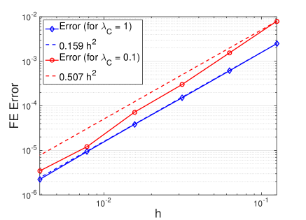
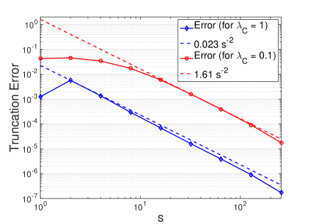
Figure 1: Estimates of the FE bias error $|\mathbb{E}[F_{h,s^{*}}-F^{*}]|$ (solid lines, left) and of the truncation error $|\mathbb{E}[F_{h^{*},s}-F^{*}]|$ (solid lines, right), as well as the bounds in (4.3) for each case (dashed lines), for $\nu=1$ and $\sigma^{2}=1$.

we plot estimates of $|\mathbb{E}[F_{h,s^{*}}-F^{*}]|$ and of $|\mathbb{E}[F_{h^{*},s}-F^{*}]|$, for the case of $d=1$, $\nu=1$, $\sigma^{2}=1$ and for two different values of $\lambda_{\mathcal{C}}$. We also show bounds over the plotted range of $h$ and $s$, for each of the two terms in (4.3) with the smallest possible values of $C_{\text{FE}}$ and of $C_{\text{trunc}}$. The expectations of these constants were estimated with $10^{5}$ MC samples and with $h^{*}=1/1024$ and $s^{*}=500$. We see that the rates of $\alpha=2=\alpha^{\prime}$ (for $\nu=1$) in (4.3) are sharp.

In our experiments, we then choose a particular sequence $\varepsilon_{L}:=2\sqrt{2}\,C_{\text{FE}}h_{L}^{2}$, where $L\geq 1$ and $C_{\text{FE}}$ is the constant in (4.3) which we estimate as shown above for each problem. We choose a corresponding truncation dimension $s_{L}$ such that $C_{\text{trunc}}s_{L}^{-2\nu/d}\leq C_{\text{FE}}h_{L}^{2}$, which implies

$$s_{L}\,:=\,\left\lceil C_{\text{bal}}\,h_{L}^{-d/\nu}\right\rceil\,\quad\text{with}\ \ C_{\text{bal}}\,:=\,(C_{\text{trunc}}/C_{\text{FE}})^{d/(2\nu)}\,,$$ (4.4)

and ensures that the total bound on the bias error in (4.3) is less than $\varepsilon_{L}/\sqrt{2}$. We then run each of the estimators until the variance error is less than $\varepsilon_{L}^{2}/2$, thus ensuring a MSE (as defined in (3.2)) of less than $\varepsilon_{L}^{2}$ and a relative standard error (as defined in (4.2)) of less than $\varepsilon_{L}/|\mathbb{E}[F]|$.

The numbers $N_{\ell}$ of lattice points for the MLQMC estimator on each of the levels are chosen adaptively using the algorithm by Giles and Waterhouse [12], given in Algorithm 1 in Section 3.3. To estimate the variance $\mathcal{V}_{\ell}:=\mathbb{V}_{\Delta}(\mathcal{Q}_{\ell}(F_{\ell}-F_{\ell-1}))$ on each level, we use (3.12). As in Corollary 2, we choose $s_{\ell}=s_{L}$ on all coarser levels. For the cost on level $\ell$, we assume

$$\mathcal{C}_{\ell}:=\mathrm{cost}(\mathcal{Q}_{\ell}(F_{\ell}-F_{\ell-1}))\approx(2s_{L}+13)\,h_{\ell}^{-1}\,N_{\ell}\,R\,.$$ (4.5)

This estimate is based on the fact (i) that the evaluation at the mid points of the mesh intervals of the coefficient in (1.2), with $a_{*}\equiv 0$, $a_{0}\equiv 1$ and with the sum truncated after $s_{L}$ terms, requires about $\mathcal{C}_{\ell}^{\text{perm}}=(2s_{L}+1)\,h_{\ell}^{-1}$ operations; and (ii) that there are direct solvers for diagonally dominant tridiagonal systems (e.g., the Thomas algorithm) that achieve a complexity of $8$ operations per unknown, leading to the cost estimate $\mathcal{C}_{\ell}^{\text{solve}}=8(h_{\ell}^{-1}+h_{\ell-1}^{-1})=12h_{\ell}^{-1}$.

For the standard MLMC estimator we choose the same mesh and truncation parameters, $h_{\ell}$ and $s_{\ell}$, as for our new MLQMC estimator. The optimal numbers of samples $N^{\text{MC}}_{\ell}$ are chosen according to the formula in the original paper [11]. This requires variance estimates for the differences $F_{\ell}-F_{\ell-1}$ on each of the levels, which are obtained via the usual sample variance estimate with $10^{2}$ initial samples, updating the estimates as $N^{\text{MC}}_{\ell}\to\infty$ on each level. The one-level variants are defined accordingly.

In Figures 2–3, we plot the cost to achieve a relative standard error less than $\varepsilon$ with MLQMC and MLMC, as well as with the one-level variants QMC and MC, for $\sigma^{2}=1$, $\nu=1,2$, and $\lambda_{\mathcal{C}}=1,0.1$. Red lines with circles correspond to the MC-based variants, while blue lines with diamonds correspond to the QMC-based estimators. The points on each graph correspond to the choices $\ell_{0}=3$ and $L=1,\ldots,4$. The values of $s_{L}$ are chosen according to (4.4) in each case. The exception is the hardest test case ($\nu=1$, $\lambda_{\mathcal{C}}=0.1$), where we used $L=2,\ldots,5$ and a variable number $s_{\ell}=\lceil C_{\text{bal}}h_{\ell}^{-1}\rceil$ of KL terms on level $\ell$ in MLQMC and in MLMC. The maximum number of KL terms included in that case is $s_{5}=456$. In all test cases, we consistently see substantial gains for the MLQMC estimator, with respect to MLMC and QMC, even though the value of $\nu$ is substantially smaller than our theory supports (see Remark 10 ahead).

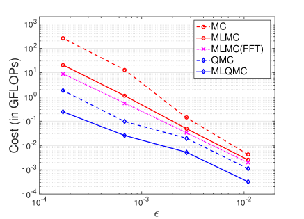
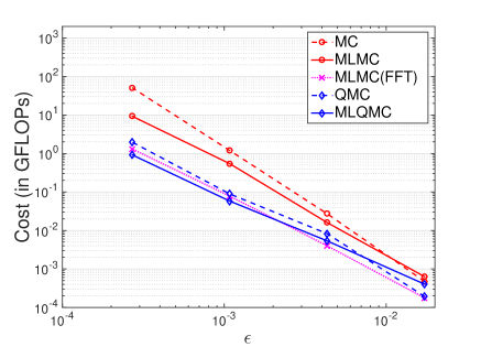
Figure 2: Cost to obtain a relative standard error less than $\varepsilon$ in the 1D example. The covariance parameters are $\nu=2$ and $\sigma^{2}=1$, as well as $\lambda_{\mathcal{C}}=1.0$ (left) and $\lambda_{\mathcal{C}}=0.1$ (right), respectively. The estimates for $C_{\text{bal}}$ are 0.76 (left) and 2.38 (right), respectively.

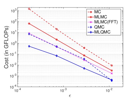
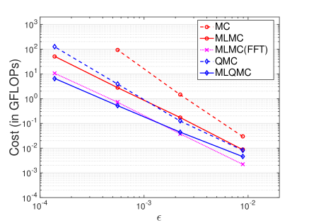
Figure 3: Cost to obtain a relative standard error less than $\varepsilon$ in the 1D example. The covariance parameters are $\nu=1$ and $\sigma^{2}=1$, as well as $\lambda_{\mathcal{C}}=1.0$ (left) and $\lambda_{\mathcal{C}}=0.1$ (right), respectively. The estimates for $C_{\text{bal}}$ are 0.38 (left) and 1.78 (right), respectively.

For comparison, we show in Figures 2–3 also cost estimates for MLMC using circulant embedding which makes use of the Fast Fourier Transform (FFT) (magenta line, labelled ‘MLMC(FFT)’). Circulant embedding allows for efficient sampling at the quadrature points from isotropic random fields, such as the one studied here, without any truncation error (see e.g. [14]) and with a cost independent of $s_{L}$. We assume that for the MLMC estimator with circulant embedding, the cost on level $\ell$ is

$$\mathcal{C}^{\text{FFT}}_{\ell}\approx\big{(}5(\ell+\ell_{0})+2\big{)}\,h_{\ell}^{-1}\,N^{\text{MC}}_{\ell}\,<\,(68/9(\ell+\ell_{0})-248/27+12)\,(\sqrt{2}h_{\ell})^{-1}\,N^{\text{MC}}_{\ell}\,.$$ (4.6)

The factor $\sqrt{2}$ in front of $h_{\ell}$ appears because there is no truncation error and thus the FE bias error can be increased by a factor 2 to still achieve a MSE of $\varepsilon_{L}^{2}$ for the MLMC estimator. For the sampling of the coefficient we then assume the use of circulant embedding without padding [14] – which doubles the number of unknowns in 1D – and a split-radix FFT algorithm that requires $\frac{34}{9}\,n\log_{2}(n)-\frac{124}{27}\,n+\mathcal{O}\big{(}\log_{2}(n)\big{)}$ operations for vectors of length $n$ [21]. This is almost certainly underestimating the cost for circulant embedding, but, as we can see in Figures 2–3, the cost is still higher than that of our MLQMC estimator asymptotically.

\psfrag{l0}{\scriptsize${\scriptstyle\bigcirc}$ $\ell=0$}\psfrag{l1}{\scriptsize$\Diamond$ $\ell=1$}\psfrag{l2}{\scriptsize${\scriptstyle\nabla}$ $\ell=2$}\psfrag{l3}{\scriptsize${\scriptstyle\triangle}$ $\ell=3$}\psfrag{l4}{\scriptsize$\Box$ $\ell=4$}\includegraphics[width=228.16034pt]{QMCerror1D_nu=1_edited.eps}

\psfrag{l0}{\scriptsize${\scriptstyle\bigcirc}$ $\ell=0$}\psfrag{l1}{\scriptsize$\Diamond$ $\ell=1$}\psfrag{l2}{\scriptsize${\scriptstyle\nabla}$ $\ell=2$}\psfrag{l3}{\scriptsize${\scriptstyle\triangle}$ $\ell=3$}\psfrag{l4}{\scriptsize$\Box$ $\ell=4$}\includegraphics[width=228.16034pt]{samples_nu=1_edited.eps}

Figure 4: Left: MSE of the QMC/MC estimators for $F_{\ell}-F_{\ell-1}$ as functions of the total number of sample points, i.e. $RN_{\ell}$ for QMC (solid blue lines) and $N_{\ell}^{\text{MC}}$ for MC (dashed red lines), for $\nu=\sigma^{2}=\lambda_{\mathcal{C}}=1$. Right: Total number of samples on each level to achieve a relative standard error less than $\varepsilon=1.8\times 10^{-4}$ for the same example.

In Figure 4, we look at the particular case $\nu=\sigma^{2}=\lambda_{\mathcal{C}}=1$, $h_{L}=1/128$ and $s_{L}=49$, and plot in the left figure the MSE of the QMC and the MC estimators for the expected values of the differences $F_{\ell}-F_{\ell-1}$ as the total number of sample points is increased (i.e., $RN_{\ell}$ and $N_{\ell}^{\text{MC}}$, respectively). We clearly see the faster rate of convergence with $N_{\ell}\to\infty$ for the QMC estimators, which is almost optimal (i.e. the MSE is nearly $\mathcal{O}(N_{\ell}^{-2})$) even though $\nu=1$ is not sufficiently big for our theory in Section 5 to apply and even though in the construction of the QMC rules we did not use the weights derived there. We also clearly see the variance reduction from level to level (i.e., the offset between the lines), which does behave as theoretically shown in Section 5 (i.e. roughly like $\mathcal{O}(h_{\ell}^{4})$).

In Figure 4 (right) we plot for the same example the numbers of sample points on each of the levels. For MLQMC they were produced by Algorithm 1, showing $RN_{\ell}$, i.e. number of lattice points times number of shifts. For standard MLMC we show two sequences of numbers: those produced by the formula in the original MLMC paper [11], labelled ‘MLMC(G)’, and those produced by Algorithm 1 with standard MC estimators on each level, labelled ‘MLMC(GW)’. We note that there are only very small differences in these final two sequences, confirming our discussion in Section 3.3 that Algorithm 1 proposed in [12] can be used instead of the original algorithm to find the optimal sample distributions over the levels. The behaviour is the same for all other parameter values.

4.2 Results in space dimension two

We consider the problem (1.1), (1.2) with Matérn covariance $\rho_{\nu}$ in (4.1) on $D=(0,1)^{2}\subset\mathbb{R}^{2}$. At first we use again homogeneous Dirichlet conditions, i.e. $\Gamma=\Gamma_{\mathcal{D}}$ and $u(\cdot,\omega)|_{\Gamma}\equiv 0$, and the source term $f\equiv 1$. The output quantity of interest is the average of the solution $u$ over the region $D^{*}=\big{(}\frac{3}{4},\frac{7}{8}\big{)}\times\big{(}\frac{7}{8},1\big{)}$, i.e.,

$$F(\omega):=\frac{1}{|D^{*}|}\,\int_{D^{*}}u(\vec{x},\omega)\,\text{d}\vec{x}\,.$$

We discretise the associated variational formulation (spatially) using standard piecewise linear, continuous FEs on a sequence of triangular meshes obtained by taking a tensor product of each of the meshes in Section 4.1 with itself and by subdividing each of the squares of the resulting mesh into two triangles, thus leading to $2^{2(\ell+\ell_{0})+1}$ triangular elements of size $h_{\ell}:=h_{0}2^{-\ell}$ with $h_{0}:=2^{-\ell_{0}+1/2}$ and $M_{\ell}=(2^{\ell+\ell_{0}}-1)^{2}$ degrees of freedom on level $\ell=0,\dots,L$.

The finite element bias error and the truncation error are estimated as in 1D. The choice of domain and functional guarantee that $u(\cdot,\omega)\in H^{2}(D)$ (almost surely) and the FE and truncation errors converge as stated in (4.3), for $\nu>1$. Then, the number of KL terms $s_{L}$ is again chosen according to (4.4) and $s_{\ell}=s_{L}$ on the coarser levels of the multilevel methods in all cases. For the average cost to compute one sample on each level, we use actual CPU-timings here (instead of FLOP counts). These were obtained using FreeFEM++ [17] and the sparse direct solver UMFPACK [8]. The measured times to evaluate the KL expansion (with $s$ terms) at the quadrature points ($\mathcal{C}_{\ell}^{\text{perm}}$) and to assemble and solve the sparse linear equation system ($\mathcal{C}_{\ell}^{\text{solve}}$) are shown in Figure 5 (left) together with the total time to compute one sample, for the case $\ell_{0}=3$, $\ell=4$ and $s=50$. Finite element methods for (1.1) in two space dimensions allow, in the practical range of $M_{\ell}$ considered here, for superior performance of sparse direct solvers as compared to, e.g., multigrid methods. Since we do not exploit the uniform grid structure in FreeFEM++ the cost in Figure 5 (left) is actually dominated by the FE system assembly, which scales like $\mathcal{O}(h_{\ell}^{-2})$. We also note that $\mathcal{C}_{\ell}^{\text{perm}}\ll\mathcal{C}_{\ell}^{\text{solve}}$ for all our choices of $s_{L}$ below.

\psfrag{l0}{\scriptsize${\scriptstyle\bigcirc}$ $\ell=0$}\psfrag{l1}{\scriptsize$\Diamond$ $\ell=1$}\psfrag{l2}{\scriptsize${\scriptstyle\nabla}$ $\ell=2$}\psfrag{l3}{\scriptsize${\scriptstyle\triangle}$ $\ell=3$}\includegraphics[width=228.16034pt]{CPUtime_sample_new.eps}

\psfrag{l0}{\scriptsize${\scriptstyle\bigcirc}$ $\ell=0$}\psfrag{l1}{\scriptsize$\Diamond$ $\ell=1$}\psfrag{l2}{\scriptsize${\scriptstyle\nabla}$ $\ell=2$}\psfrag{l3}{\scriptsize${\scriptstyle\triangle}$ $\ell=3$}\includegraphics[width=228.16034pt]{QMCerror_15_1_64_edited.eps}

Figure 5: Left: Measured CPU times to calculate one sample of $F_{\ell}$ on level $\ell$ for the 2D problem with $\ell_{0}=3$ and $s=50$. Right: MSE of the QMC/MC estimators for $\mathbb{E}[F_{\ell}-F_{\ell-1}]$, as functions of the number of sample points, i.e. $RN_{\ell}$ for QMC (solid blue lines) and $N^{\text{MC}}_{\ell}$ for MC (dashed red lines), for $\nu=1.5$, $\sigma^{2}=1$, $\lambda_{\mathcal{C}}=1$, $\ell_{0}=3$, $L=3$ and $s_{L}=27$.

In Figure 5 (right), we plot the MSE of the QMC and of the MC estimators for $\mathbb{E}[F_{\ell}-F_{\ell-1}]$ as a function of the total number of sample points for the covariance parameters $\nu=1.5$, $\sigma^{2}=1$, $\lambda_{\mathcal{C}}=1$, and for $\ell_{0}=3$, $L=3$ and $s_{L}=27$. Again, we see the significantly faster and almost optimal convergence rate for the QMC estimators as $N_{\ell}\to\infty$.

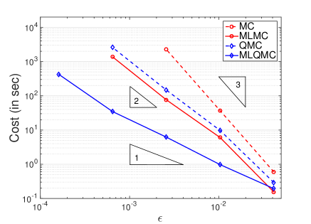
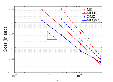
Figure 6: Cost to obtain a relative standard error less than $\varepsilon$ in the 2D example with homogeneous Dirichlet conditions, for $\nu=2.5$, $\sigma^{2}=0.25$, $\lambda_{\mathcal{C}}=1$ and $\ell_{0}=3$ (left), as well as for $\nu=1.5$, $\sigma^{2}=1$, $\lambda_{\mathcal{C}}=0.1$ and $\ell_{0}=4$ (right). The estimates for $C_{\text{bal}}$ are 0.55 (left) and 0.68 (right), leading to a maximum of $s_{5}=47$ and $s_{4}=1106$ KL terms on the finest mesh, respectively.

In Figure 6, we plot again the cost to achieve a relative standard error less than $\varepsilon$ with all four estimators for two sets of covariance parameters. The points on each of the graphs correspond to the choices $L=1,\ldots,5$ with $\ell_{0}=3$ (left) and $L=1,\ldots,4$ with $\ell_{0}=4$ (right). We see similarly impressive gains with respect to MLMC and QMC in two dimensions, but we also see more clearly the influence of the smoothness parameter $\nu$. For the test case in the left figure, the numerically observed growth of the MLQMC cost is about $\mathcal{O}(\varepsilon^{-1.25})$ over the range $L=1$ to $4$. For comparison, the costs for MLMC and QMC both show growths of $\mathcal{O}(\varepsilon^{-2.2})$ over the same range, while MC shows the expected $\mathcal{O}(\varepsilon^{-3})$ growth.

As a final example, we consider the practically more interesting case of a 2D “flow cell”, that is, we solve the PDE (1.1) in $D=(0,1)^{2}$ with mixed Dirichlet–Neumann conditions. The horizontal boundaries are assumed to be impermeable, that is, $(a\nabla u)\cdot\vec{n}=0$ for $x_{2}=0$ and $x_{2}=1$. Along the vertical boundaries we specify Dirichlet boundary conditions and set $u\equiv 1$, for $x_{1}=0$, and $u\equiv 0$, for $x_{1}=1$. We discretise this problem using the same sequence of meshes as above. Due to the Neumann conditions on the horizontal boundaries, the number of degrees of freedom in this problem is $M_{\ell}=2^{2(\ell+\ell_{0})}-1$ on level $\ell=0,\dots,L$.

Here, the quantity of interest is the outflow through the right vertical boundary, i.e.

$$F(\omega):=-\int_{0}^{1}a(\vec{x},\omega)\frac{\partial u(\vec{x},\omega)}{\partial x_{1}}\bigg{|}_{x_{1}=1}\ \mathrm{d}x_{2}\;.$$

As an approximation of this functional we use

$$F_{h,s}(\omega):=-\int_{D}a_{s}(\vec{x},\omega)\nabla u_{h,s}(\vec{x},\omega)\cdot\nabla\varphi(\vec{x})\ \mathrm{d}\vec{x},$$

where $\varphi$ denotes the FE function which is equal to one at all of the vertices of the right vertical boundary and is equal to zero at all other vertices (see [34, section 3.4] for details).

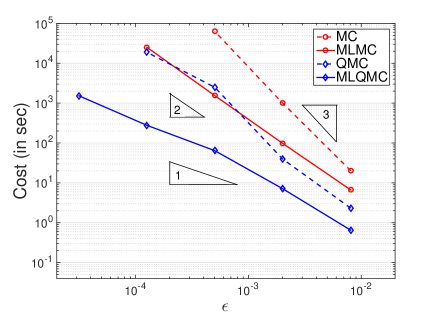
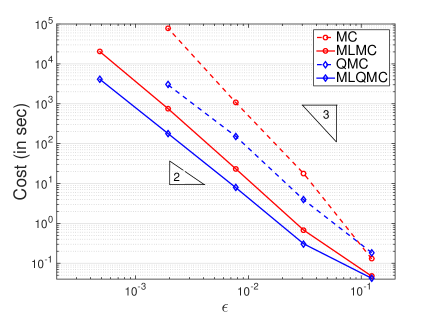
Figure 7: Cost to obtain a relative standard error less than $\varepsilon$ in the 2D flow cell example. The covariance parameters are $\nu=2.5$, $\sigma^{2}=1$, $\lambda_{\mathcal{C}}=1$ (left) and $\nu=1$, $\sigma^{2}=3$, $\lambda_{\mathcal{C}}=0.3$ (right). The estimates for $C_{\text{bal}}$ are 0.61 (left) and 0.0097 (right), respectively. The problem on the right is significantly more challenging. Please note the different range for $\varepsilon$ in the two figures.

The numerical results for this problem are shown in Figure 7. In the left figure, we choose $\nu=2.5$, $\sigma^{2}=1$, $\lambda_{\mathcal{C}}=1$. In the right figure, we choose a set of parameters closer to the ones used in actual subsurface flow studies, namely $\nu=1$, $\sigma^{2}=3$ and $\lambda_{\mathcal{C}}=0.3$. In both cases $\ell_{0}=2$. The points on the graphs correspond to the choices $L=1,\ldots,5$ (left) and $L=2,\ldots,5$ (right), respectively. The gains are again of the same order as above in both cases. In the smoother test case (left), the growth of the MLQMC cost is as low as $\mathcal{O}(\varepsilon^{-1.15})$ between $L=3$ and $5$.

5 Mathematical analysis and construction of suitable QMC rules

In the remainder of the paper, we present sufficient conditions on the data and on the FE spaces to verify Assumption M2 in the general MLQMC convergence result in Theorem 1, as well as constructible QMC rules that achieve this. We will start in Section 5.1 by addressing the spatial regularity and approximation orders for the FE function $u_{h,s}(\cdot,{\boldsymbol{y}})$ in (1.5), making explicit the dependence on the parameter ${\boldsymbol{y}}$ in any constants that appear. Then we turn to the key estimates required for the MLQMC theory: bounds on the derivatives of the FE error with respect to the stochastic variables in certain weighted function spaces $\mathcal{W}_{s}$ which appear in the QMC convergence theory (see [13] and the references there) with constants that are independent of the truncation dimension $s$. These bounds correspond to “mixed derivative bounds”, appearing also in hyperbolic cross and other high-dimensional approximation methods [3, 31, 16], in that they require joint regularity of the random solution $u(\vec{x},\omega)$ with respect to the spatial as well as with respect to the stochastic argument. These estimates are proved in Section 5.2, and are used in Section 5.3 to establish the MLQMC convergence rate estimates.

5.1 Parametric formulation, spatial regularity and FE approximation

As in [13], we assume that, for $d=2,\,3$, $D$ is a bounded, Lipschitz polygonal/polyhedral domain. For simplicity, we restrict ourselves to homogeneous Dirichlet data $\phi_{\mathcal{D}}=0$ and to deterministic Neumann data $\phi_{\mathcal{N}}\in H^{1/2}(\Gamma_{\mathcal{N}})$ in (1.1). Then, the stochastic PDE (1.1) is (upon a measure-zero modification of the lognormal random field $a$ in (1.1)), equivalent to the infinite-dimensional, parametric, deterministic PDE

$$-\nabla\cdot(a(\cdot,{\boldsymbol{y}})\,\nabla u(\cdot,{\boldsymbol{y}}))\,=\,f\quad\mbox{in}\quad D,\quad u|_{\Gamma_{\mathcal{D}}}\,=\,0,\quad\vec{n}\cdot a(\cdot,{\boldsymbol{y}})\nabla u(\cdot,{\boldsymbol{y}})|_{\Gamma_{\mathcal{N}}}\,=\,\phi_{\mathcal{N}}\,,$$ (5.1)

with parametric, deterministic coefficient

$$a(\vec{x},{\boldsymbol{y}})\,=\,a_{*}(\vec{x})+a_{0}(\vec{x})\exp\bigg{(}\sum_{j\geq 1}\sqrt{\mu_{j}}\,\xi_{j}(\vec{x})\,y_{j}\bigg{)}\,,$$ (5.2)

where $\vec{x}\in D\subset\mathbb{R}^{d}$ and where the parameter sequence ${\boldsymbol{y}}=(y_{j})_{j\geq 1}\in\mathbb{R}^{\mathbb{N}}$ is distributed according to the product Gaussian measure $\overline{\boldsymbol{\mu}}_{G}=\bigotimes_{j=1}^{\infty}\mathcal{N}(0,1)$.

If ${\boldsymbol{y}}$ belongs to the set

$$U_{{\boldsymbol{b}}}\,:=\,\bigg{\{}{\boldsymbol{y}}\in\mathbb{R}^{\mathbb{N}}\;:\;\sum_{j\geq 1}b_{j}\,|y_{j}|<\infty\bigg{\}}\subset\mathbb{R}^{\mathbb{N}}\,,$$ (5.3)

where the sequence ${\boldsymbol{b}}=(b_{j})_{j\geq 1}$ is defined by $b_{j}\,:=\,\sqrt{\mu_{j}}\,\|\xi_{j}\|_{L^{\infty}(D)}$ and is assumed to be in $\ell^{2}(\mathbb{N})$, then the equivalence of (5.1)–(5.2) and (1.1)–(1.2) holds up to $\overline{\boldsymbol{\mu}}_{G}$-measure zero modifications of the input random field. Due to the continuous dependence on the input random field, the parametric, deterministic coefficient $a(\cdot,{\boldsymbol{y}})$ in (5.2) and the parametric, deterministic solution $u(\cdot,{\boldsymbol{y}})$ of (5.1) will also differ only on a $\overline{\boldsymbol{\mu}}_{G}$-nullset. If, moreover, ${\boldsymbol{b}}\in\ell^{1}(\mathbb{N})$, then the series (5.2) converges in $L^{\infty}(D)$ for every ${\boldsymbol{y}}\in U_{\boldsymbol{b}}$, which we assume in what follows.

To simplify the presentation, we assume $a_{*}=0$ and $|\Gamma_{\mathcal{D}}|>0$. We need the weak form of (5.1) on the Hilbert space $V=H^{1}_{\Gamma_{\mathcal{D}}}(D):=\{v\in H^{1}(D):v|_{\Gamma_{\mathcal{D}}}=0\}$, with norm

$$\|v\|_{V}\,:=\,\|\nabla v\|_{L^{2}(D)}\,.$$

As in [13], we define for ${\boldsymbol{y}}\in U_{\boldsymbol{b}}$ the parametric, deterministic bilinear form in $V$ by

$${\mathscr{A}}({\boldsymbol{y}};w,v)\,:=\,\int_{D}a(\vec{x},{\boldsymbol{y}})\,\nabla w(\vec{x})\cdot\nabla v(\vec{x})\,\mathrm{d}\vec{x}\,,\qquad\mbox{for all}\quad w,v\in V\,.$$ (5.4)

We list properties of the parametric bilinear form ${\mathscr{A}}({\boldsymbol{y}};\cdot,\cdot)$ and of the weak solution $u(\cdot,{\boldsymbol{y}})$, as well as its FE approximation $u_{h}(\cdot,{\boldsymbol{y}})$, from [13]. For a proof see [13, Thm. 13].

Proposition 3

Assume that ${\boldsymbol{b}}\in\ell^{1}(\mathbb{N})$.

1. The expressions

   $$\hat{a}({\boldsymbol{y}})\,:=\,\max_{\vec{x}\in\overline{D}}a(\vec{x},{\boldsymbol{y}})\quad\mbox{and}\quad\check{a}({\boldsymbol{y}})\,:=\,\min_{\vec{x}\in\overline{D}}a(\vec{x},{\boldsymbol{y}})$$ (5.5)

   are well-defined, $\overline{\boldsymbol{\mu}}_{G}$-measurable mappings from $U_{\boldsymbol{b}}$ to $\mathbb{R}$ which satisfy

   $$0<\check{a}({\boldsymbol{y}})\leq\hat{a}({\boldsymbol{y}})<\infty\qquad\text{for all}\quad{\boldsymbol{y}}\in U_{\boldsymbol{b}}\,.$$ (5.6)

2. For every ${\boldsymbol{y}}\in U_{\boldsymbol{b}}$, the parametric bilinear form ${\mathscr{A}}({\boldsymbol{y}};\cdot,\cdot):V\times V\rightarrow\mathbb{R}$ defined in (5.4) is continuous and coercive in the following sense:

   $${\mathscr{A}}({\boldsymbol{y}};w,w) \,\geq\,\check{a}({\boldsymbol{y}})\|w\|_{V}^{2} \text{for all}\quad w\in V\,,\quad\mbox{and}$$ (5.7)

   $${\mathscr{A}}({\boldsymbol{y}};v,w) \,\leq\,\hat{a}({\boldsymbol{y}})\|v\|_{V}\|w\|_{V} \text{for all}\quad v,w\in V\,.$$ (5.8)

3. For every $f\in L^{2}(D)$ and every $\phi_{\mathcal{N}}\in H^{1/2}(\Gamma_{\mathcal{N}})$ and with the (${\boldsymbol{y}}$-independent) linear functional

   $${\mathscr{L}}(v)\,:=\,\int_{D}f(\vec{x})\,v(\vec{x})\,\mathrm{d}\vec{x}+\int_{\Gamma_{\mathcal{N}}}\phi_{\mathcal{N}}(\vec{x})\,v(\vec{x})\,\mathrm{d}s\,,$$

   the parametric, deterministic variational problem, to find $u(\cdot,{\boldsymbol{y}})\in V$ such that

   $${\mathscr{A}}({\boldsymbol{y}};u(\cdot,{\boldsymbol{y}}),v)\,=\,{\mathscr{L}}(v)\qquad\mbox{for all}\quad v\in V\,,$$ (5.9)

   admits a unique solution $u(\cdot,{\boldsymbol{y}})\in V$, for every ${\boldsymbol{y}}\in U_{\boldsymbol{b}}$.

4. This parametric solution $U_{\boldsymbol{b}}\ni{\boldsymbol{y}}\mapsto u(\cdot,{\boldsymbol{y}})\in V$ is a strongly measurable mapping (with respect to a suitable $\sigma$-algebra, cf. [13]) which satisfies the bound

   $$\|u(\cdot,{\boldsymbol{y}})\|_{V}\,\lesssim\,\frac{1}{\check{a}({\boldsymbol{y}})}\left(\|f\|_{L^{2}(D)}+\|\phi_{\mathcal{N}}\|_{H^{1/2}(\Gamma_{\mathcal{N}})}\right)\qquad\text{for all}\quad{\boldsymbol{y}}\in U_{\boldsymbol{b}}\,,$$ (5.10)

   (pointwise with respect to ${\boldsymbol{y}}$). The implied constant depends on $D$, $\Gamma_{\mathcal{D}}$ and $\Gamma_{\mathcal{N}}$, but is independent of ${\boldsymbol{y}}$. In particular, for any $s\in\mathbb{N}$, $u(\cdot,({\boldsymbol{y}}_{\{1:s\}};\boldsymbol{0}))\in V$ is well-defined, measurable, and satisfies the above bounds uniformly with respect to $s$.

5. Restricting in (5.9) to functions in the FE space $V_{h}\subset V$, there exists a unique, parametric FE solution $u_{h}(\cdot,{\boldsymbol{y}})\in V_{h}$, for every ${\boldsymbol{y}}\in U_{\boldsymbol{b}}$ and $0<h<1$, that also satisfies the bound (5.10). Replacing, in addition, the coefficient $a(\vec{x},{\boldsymbol{y}})$ in (5.9) by the $s$-term truncated KL expansion $a^{s}(\vec{x},{\boldsymbol{y}})$, the corresponding $s$-parametric FE solutions $u_{h,s}(\cdot,({\boldsymbol{y}}_{\{1:s\}};\boldsymbol{0}))\in V_{h}$ are uniquely defined for any ${\boldsymbol{y}}_{\{1:s\}}\in\mathbb{R}^{s}$, and satisfy, for $({\boldsymbol{y}}_{\{1:s\}};\boldsymbol{0})\in U_{\boldsymbol{b}}$, the bound (5.10) uniformly with respect to $h$ and to $s$.

For the derivation of FE convergence rate bounds, we require additional spatial regularity: we assume in (5.2)

$$a_{*}\equiv 0\,,\quad a_{0}\in W^{1,\infty}(D)\quad\text{and}\quad\xi_{j}\in W^{1,\infty}(D)\,.$$ (5.11)

With (5.11), we may define the sequence

$$\overline{b}_{j}\,:=\,\sqrt{\mu_{j}}\,\max(\|\xi_{j}\|_{L^{\infty}(D)},\||\nabla\xi_{j}|\|_{L^{\infty}(D)})\,,\quad j=1,2,...\,.$$ (5.12)

Evidently, $\overline{b}_{j}\geq b_{j}$ so that $U_{\overline{{\boldsymbol{b}}}}\subset U_{{\boldsymbol{b}}}\subset\mathbb{R}^{\mathbb{N}}$. We assume in what follows that

$$\overline{{\boldsymbol{b}}}=(\overline{b}_{j})_{j\geq 1}\in\ell^{1}(\mathbb{N})\;.$$ (5.13)

These conditions are satisfied under the provision of appropriate regularity of the covariance function of the Gaussian random field $\log(a-a_{*})$ in (1.1) (we refer to the discussion in [13, Rem. 4]). Also, for any $\overline{{\boldsymbol{b}}}\in\ell^{1}(\mathbb{N})\subset\ell^{2}(\mathbb{N})$ we have $\overline{\boldsymbol{\mu}}_{G}(U_{\overline{{\boldsymbol{b}}}})=1$.

Proposition 4

Let us assume (5.11) and (5.13), and suppose we are given deterministic functions $f\in L^{2}(D)$ and $\phi_{\mathcal{N}}\in H^{1/2}(\Gamma_{\mathcal{N}})$. Then the following results hold.

1. For every ${\boldsymbol{y}}\in U_{\overline{{\boldsymbol{b}}}}$ , the series (5.2) converges in $W^{1,\infty}(D)$ and

   $$a(\cdot,{\boldsymbol{y}})\in W^{1,\infty}(D)\,.$$ (5.14)

2. The parametric solution map ${\boldsymbol{y}}\mapsto u(\cdot,{\boldsymbol{y}})$ is strongly $\overline{\boldsymbol{\mu}}_{G}$–measurable as a map from $U_{\overline{{\boldsymbol{b}}}}$ to the space

   $$W\,:=\,\{v\in V:\Delta u\in L^{2}(D)\}\,,$$ (5.15)

   and we have the a priori estimate

   $$\|\Delta u(\cdot,{\boldsymbol{y}})\|_{L^{2}(D)}\,\lesssim\,T_{1}({\boldsymbol{y}})\left(\|f\|_{L^{2}(D)}+\|\phi_{\mathcal{N}}\|_{H^{1/2}(\Gamma_{\mathcal{N}})}\right),$$ (5.16)

   where

   $$T_{1}({\boldsymbol{y}})\,:=\,\frac{1}{\check{a}({\boldsymbol{y}})}+\frac{\|\nabla a(\cdot,{\boldsymbol{y}})\|_{L^{\infty}(D)}}{\check{a}({\boldsymbol{y}})^{2}}\,<\,\infty\qquad\mbox{for all}\quad{\boldsymbol{y}}\in U_{\overline{{\boldsymbol{b}}}}\,.$$ (5.17)

3. There exists a sequence $\{V_{h_{\ell}}\}_{\ell\geq 0}$ of nested FE spaces of continuous, piecewise linear functions on conforming, simplicial meshes $\{\mathcal{T}_{h_{\ell}}\}_{\ell\geq 0}$ that satisfies the assumptions of Section 3: in particular, $M_{\ell}=\mathrm{dim}(V_{h_{\ell}})\eqsim h_{\ell}^{-d}$ and $h_{\ell}\eqsim 2^{-\ell}$. The solutions $u_{h_{\ell}}(\cdot,{\boldsymbol{y}})\in V_{h_{\ell}}$ defined in Proposition 3 (e) satisfy the asymptotic error bound

   $$\|a^{1/2}(\cdot,{\boldsymbol{y}})\,\nabla(u-u_{h_{\ell}})(\cdot,{\boldsymbol{y}})\|_{L^{2}(D)}\,\lesssim\,h_{\ell}\,T_{2}({\boldsymbol{y}})\,\|\Delta u(\cdot,{\boldsymbol{y}})\|_{L^{2}(D)}\,,$$ (5.18)

   where

   $$T_{2}({\boldsymbol{y}})\,:=\,\hat{a}({\boldsymbol{y}})^{1/2}\qquad\mbox{for all}\quad{\boldsymbol{y}}\in U_{\overline{{\boldsymbol{b}}}}\,.$$ (5.19)

   The result holds verbatim for the FE solution $u_{h_{\ell},s_{\ell}}(\cdot,({\boldsymbol{y}}_{\{1:s_{\ell}\}},\boldsymbol{0}))\in V_{h_{\ell}}$ of the $s_{\ell}$-term truncated problem.

Proof.

(a)  This is a consequence of (5.13) and $\overline{\boldsymbol{\mu}}_{G}(U_{\overline{{\boldsymbol{b}}}})=1$ (see, eg., [31, Lem. 2.28]).

(b)  Since $a(\cdot,{\boldsymbol{y}})\in W^{1,\infty}(D)$, $u|_{\Gamma_{\mathcal{D}}}=0$ and (5.6) holds, for every ${\boldsymbol{y}}\in U_{\overline{{\boldsymbol{b}}}}$, the solution $u(\cdot,{\boldsymbol{y}})$ of (5.1) also satisfies the following Poisson problem

$$-\Delta u(\cdot,{\boldsymbol{y}})\,=\,\tilde{f}(\cdot,{\boldsymbol{y}})\,:=\,\frac{1}{a(\cdot,{\boldsymbol{y}})}\left[f+\nabla a(\cdot,{\boldsymbol{y}})\cdot\nabla u(\cdot,{\boldsymbol{y}})\right]\quad\mbox{in}\ L^{2}(D)\,,$$ (5.20)

The bound (5.16) with $T_{1}({\boldsymbol{y}})$ defined in (5.17) then follows from (5.10).

(c)  The bound on $\|\Delta u(\cdot,{\boldsymbol{y}})\|_{L^{2}(D)}$ in (b) together with the classical regularity theory for the Laplace operator on Lipschitz polygonal/polyhedral domains (see, e.g., [15]) implies weighted $H^{2}(D)$-regularity of $u(\cdot,{\boldsymbol{y}})$ (with suitable weights near reentrant corners and edges) for non-convex $D$ and full $H^{2}(D)$-regularity for convex $D$. The existence of a sequence $\{V_{h_{\ell}}\}_{\ell\geq 0}$ that satisfies the assumptions of Section 3, together with

$$\inf_{v\in V_{h_{\ell}}}\|w-v\|_{V}\,\lesssim\,h_{\ell}\,\|\Delta w\|_{L^{2}(D)}\qquad\text{for all}\quad w\in W\,,$$ (5.21)

then follows from classical FE results (for convergence bounds in weighted spaces see, e.g., [1]) and from the norm equivalence $\|\Delta w\|_{L^{2}(D)}\eqsim\|w\|_{W}$, for all $w\in W$. The error bound in (5.18) follows from an application of Cea’s Lemma [15] (in the energy norm) together with (5.8) and (5.21). ∎

Note that, for convex $D$ and for homogeneous Dirichlet boundary conditions on all of $\partial D$, $W=H^{2}(D)$ and the family $\{\mathcal{T}_{h_{\ell}}\}_{\ell\geq 0}$ can be constructed by uniform mesh refinement of an arbitrary conforming triangulation $\mathcal{T}_{h_{0}}$ of $D$.

5.2 Parametric Regularity

As first observed in [24], in the uniform case, the analysis of MLQMC methods for FE discretisations of PDEs requires estimates of the parametric solution map ${\boldsymbol{y}}\mapsto u(\cdot,{\boldsymbol{y}})$ in the regularity space $W$ in (5.15). Here, we establish corresponding results for the lognormal parametric problem (5.1), (5.2). In order to be able to draw upon our results in [13], we restrict the analysis to the particular case

$$\Gamma_{\mathcal{N}}=\emptyset,\quad\Gamma_{\mathcal{D}}=\Gamma,\quad V=H^{1}_{0}(D),\quad\text{and}\ \ V^{*}=H^{-1}(D)\;.$$ (5.22)

We denote by ${\mathfrak{F}}\,:=\,\{{\boldsymbol{\nu}}\in\mathbb{N}_{0}^{\mathbb{N}}\;:\;|{\boldsymbol{\nu}}|<\infty\}$, where $|{\boldsymbol{\nu}}|:=\sum_{j=1}\nu_{j}$, the (countable) set of all “finitely supported” multi-indices (i.e., sequences of nonnegative integers for which only finitely many entries are nonzero). For ${\boldsymbol{m}},{\boldsymbol{\nu}}\in{\mathfrak{F}}$, we write ${\boldsymbol{m}}\leq{\boldsymbol{\nu}}$ if $m_{j}\leq\nu_{j}$ for all $j$, we denote by ${\boldsymbol{\nu}}-{\boldsymbol{m}}$ a multi-index with the elements $\nu_{j}-m_{j}$, and we define $\binom{{\boldsymbol{\nu}}}{{\boldsymbol{m}}}:=\prod_{j\geq 1}\binom{\nu_{j}}{m_{j}}$. For a sequence of non-negative real numbers $(\beta_{j})_{j\in\mathbb{N}}$ we write ${\boldsymbol{\beta}}^{\boldsymbol{\nu}}:=\prod_{j\geq 1}\beta_{j}^{\nu_{j}}$. The following result is abstracted from the proof of [13, Thm. 14].

Lemma 5

Given non-negative numbers $(\beta_{j})_{j\in\mathbb{N}}$, let $(\mathbb{A}_{\boldsymbol{\nu}})_{{\boldsymbol{\nu}}\in{\mathfrak{F}}}$ and $(\mathbb{B}_{\boldsymbol{\nu}})_{{\boldsymbol{\nu}}\in{\mathfrak{F}}}$ be non-negative numbers satisfying the inequality

$$\mathbb{A}_{\boldsymbol{\nu}}\,\leq\,\sum_{\stackrel{{\scriptstyle\scriptstyle{{\boldsymbol{m}}\leq{\boldsymbol{\nu}}}}}{{\scriptstyle{{\boldsymbol{m}}\neq{\boldsymbol{\nu}}}}}}\binom{{\boldsymbol{\nu}}}{{\boldsymbol{m}}}{\boldsymbol{\beta}}^{{\boldsymbol{\nu}}-{\boldsymbol{m}}}\mathbb{A}_{\boldsymbol{m}}+\mathbb{B}_{\boldsymbol{\nu}}\,,\quad\mbox{for any ${\boldsymbol{\nu}}\in{\mathfrak{F}}$ {(}including ${\boldsymbol{\nu}}={\boldsymbol{0}}${)}}.$$

Then

$$\mathbb{A}_{\boldsymbol{\nu}}\,\leq\,\sum_{{\boldsymbol{k}}\leq{\boldsymbol{\nu}}}\binom{{\boldsymbol{\nu}}}{{\boldsymbol{k}}}\Lambda_{|{\boldsymbol{k}}|}\,{\boldsymbol{\beta}}^{\boldsymbol{k}}\,\mathbb{B}_{{\boldsymbol{\nu}}-{\boldsymbol{k}}}\,,\quad\mbox{for all ${\boldsymbol{\nu}}\in{\mathfrak{F}}$},$$

where the sequence $(\Lambda_{n})_{n\geq 0}$ is defined recursively by

$$\Lambda_{0}\,:=\,1\quad\mbox{and}\quad\Lambda_{n}\,:=\,\sum_{i=0}^{n-1}\binom{n}{i}\Lambda_{i}\,,\quad\mbox{for all $n\geq 1$}.$$ (5.23)

The result holds also when both inequalities are replaced by equalities. Moreover, we have

$$\Lambda_{n}\,\leq\,\frac{n!}{(\log 2)^{n}}\,,\quad\mbox{for all \ $n\geq 0$}.$$ (5.24)

Proof.

We prove this result by induction. The case ${\boldsymbol{\nu}}={\boldsymbol{0}}$ holds trivially. Suppose that the result holds for all $|{\boldsymbol{\nu}}|<n$ with some $n\geq 1$. Then for $|{\boldsymbol{\nu}}|=n$, we substitute ${\boldsymbol{m}}^{\prime}={\boldsymbol{\nu}}-{\boldsymbol{m}}$ in the recursion and use the induction hypothesis to write

$$\mathbb{A}_{\boldsymbol{\nu}} \,\leq\,\sum_{{\boldsymbol{0}}\neq{\boldsymbol{m}}^{\prime}\leq{\boldsymbol{\nu}}}\binom{{\boldsymbol{\nu}}}{{\boldsymbol{\nu}}-{\boldsymbol{m}}^{\prime}}\beta^{{\boldsymbol{m}}^{\prime}}\mathbb{A}_{{\boldsymbol{\nu}}-{\boldsymbol{m}}^{\prime}}+\mathbb{B}_{\boldsymbol{\nu}}$$

$$\,\leq\,\sum_{{\boldsymbol{0}}\neq{\boldsymbol{m}}^{\prime}\leq{\boldsymbol{\nu}}}\binom{{\boldsymbol{\nu}}}{{\boldsymbol{\nu}}-{\boldsymbol{m}}^{\prime}}\beta^{{\boldsymbol{m}}^{\prime}}\sum_{{\boldsymbol{k}}\leq{\boldsymbol{\nu}}-{\boldsymbol{m}}^{\prime}}\binom{{\boldsymbol{\nu}}-{\boldsymbol{m}}^{\prime}}{{\boldsymbol{k}}}\Lambda_{|{\boldsymbol{k}}|}\,\beta^{\boldsymbol{k}}\,\mathbb{B}_{{\boldsymbol{\nu}}-{\boldsymbol{m}}^{\prime}-{\boldsymbol{k}}}+\mathbb{B}_{\boldsymbol{\nu}}.$$

Substituting ${\boldsymbol{k}}^{\prime}={\boldsymbol{k}}+{\boldsymbol{m}}^{\prime}$, exchanging the order of summation, and regrouping the binomial coefficients, we obtain

$$\mathbb{A}_{\boldsymbol{\nu}} \,\leq\,\sum_{{\boldsymbol{0}}\neq{\boldsymbol{m}}^{\prime}\leq{\boldsymbol{\nu}}}\binom{{\boldsymbol{\nu}}}{{\boldsymbol{\nu}}-{\boldsymbol{m}}^{\prime}}\sum_{{\boldsymbol{m}}^{\prime}\leq{\boldsymbol{k}}^{\prime}\leq{\boldsymbol{\nu}}}\binom{{\boldsymbol{\nu}}-{\boldsymbol{m}}^{\prime}}{{\boldsymbol{k}}^{\prime}-{\boldsymbol{m}}^{\prime}}\Lambda_{|{\boldsymbol{k}}^{\prime}-{\boldsymbol{m}}^{\prime}|}\,\beta^{{\boldsymbol{k}}^{\prime}}\,\mathbb{B}_{{\boldsymbol{\nu}}-{\boldsymbol{k}}^{\prime}}+\mathbb{B}_{\boldsymbol{\nu}}$$

$$\,=\,\sum_{{\boldsymbol{0}}\neq{\boldsymbol{k}}^{\prime}\leq{\boldsymbol{\nu}}}\binom{{\boldsymbol{\nu}}}{{\boldsymbol{k}}^{\prime}}\sum_{{\boldsymbol{0}}\neq{\boldsymbol{m}}^{\prime}\leq{\boldsymbol{k}}^{\prime}}\binom{{\boldsymbol{k}}^{\prime}}{{\boldsymbol{k}}^{\prime}-{\boldsymbol{m}}^{\prime}}\Lambda_{|{\boldsymbol{k}}^{\prime}-{\boldsymbol{m}}^{\prime}|}\,\beta^{{\boldsymbol{k}}^{\prime}}\,\mathbb{B}_{{\boldsymbol{\nu}}-{\boldsymbol{k}}^{\prime}}+\mathbb{B}_{\boldsymbol{\nu}},$$

where

$$\sum_{{\boldsymbol{0}}\neq{\boldsymbol{m}}\leq{\boldsymbol{k}}^{\prime}}\binom{{\boldsymbol{k}}^{\prime}}{{\boldsymbol{k}}^{\prime}-{\boldsymbol{m}}}\Lambda_{|{\boldsymbol{k}}^{\prime}-{\boldsymbol{m}}|} \,=\,\sum_{\stackrel{{\scriptstyle\scriptstyle{{\boldsymbol{m}}\leq{\boldsymbol{k}}^{\prime}}}}{{\scriptstyle{{\boldsymbol{m}}\neq{\boldsymbol{k}}^{\prime}}}}}\binom{{\boldsymbol{k}}^{\prime}}{{\boldsymbol{m}}}\Lambda_{|{\boldsymbol{m}}|}\,=\,\sum_{i=0}^{|{\boldsymbol{k}}^{\prime}|-1}\sum_{\stackrel{{\scriptstyle\scriptstyle{{\boldsymbol{m}}\leq{\boldsymbol{k}}^{\prime}}}}{{\scriptstyle{|{\boldsymbol{m}}|=i}}}}\binom{{\boldsymbol{k}}^{\prime}}{{\boldsymbol{m}}}\Lambda_{i}\,=\,\sum_{i=0}^{|{\boldsymbol{k}}^{\prime}|-1}\binom{|{\boldsymbol{k}}^{\prime}|}{i}\Lambda_{i}\,,$$

which is equal to $\Lambda_{|{\boldsymbol{k}}^{\prime}|}$ as required. In the last step we used a simple counting identity (consider the number of ways to select $i$ distinct balls from some baskets containing a total number of $|{\boldsymbol{k}}^{\prime}|$ distinct balls)

$$\sum_{\stackrel{{\scriptstyle\scriptstyle{{\boldsymbol{m}}\leq{\boldsymbol{k}}^{\prime}}}}{{\scriptstyle{|{\boldsymbol{m}}|=i}}}}\binom{{\boldsymbol{k}}^{\prime}}{{\boldsymbol{m}}}\,=\,\binom{|{\boldsymbol{k}}^{\prime}|}{i}\,.$$ (5.25)

The proof of (5.24) then follows as in the proof of [13, Thm. 14]. ∎

Theorem 6

For every $f\in L^{2}(D)$, ${\boldsymbol{\nu}}\in{\mathfrak{F}}$ and ${\boldsymbol{y}}\in U_{\overline{{\boldsymbol{b}}}}$, with $T_{1}({\boldsymbol{y}})$ as in (5.17), we have

$$\|\Delta(\partial^{\boldsymbol{\nu}}u(\cdot,{\boldsymbol{y}}))\|_{L^{2}(D)}\;\lesssim\;\|f\|_{L^{2}(D)}\,T_{1}({\boldsymbol{y}})\,\overline{{\boldsymbol{b}}}^{{\boldsymbol{\nu}}}\,2^{|{\boldsymbol{\nu}}|}\,(|{\boldsymbol{\nu}}|+1)!\,.$$

Proof.

Throughout this proof, all estimates are for arbitrary ${\boldsymbol{y}}\in U_{\bar{{\boldsymbol{b}}}}\subset U_{{\boldsymbol{b}}}$ with the understanding that constants implied in $\simeq$ and $\lesssim$ do not depend on ${\boldsymbol{y}}$. For any multi-index ${\boldsymbol{\nu}}\in{\mathfrak{F}}$, we define (formally, at this stage) the expression

$$g_{\boldsymbol{\nu}}(\cdot,{\boldsymbol{y}})\,:=\,\nabla\cdot(a(\cdot,{\boldsymbol{y}})\,\nabla(\partial^{\boldsymbol{\nu}}u(\cdot,{\boldsymbol{y}})))\,.$$

Differentiation of order $|{\boldsymbol{\nu}}|>0$ of the parametric, deterministic variational formulation (5.9) with respect to ${\boldsymbol{y}}$ reveals that

$$0\,=\,\partial^{\boldsymbol{\nu}}\,{\mathscr{A}}({\boldsymbol{y}};u(\cdot,{\boldsymbol{y}}),v)\,=\,\int_{D}\nabla v(\vec{x})\cdot\partial^{\boldsymbol{\nu}}\big{(}a(\vec{x},{\boldsymbol{y}})\nabla u(\vec{x},{\boldsymbol{y}})\big{)}\,\mathrm{d}\vec{x}\qquad\text{for all}\quad v\in V\,.$$

The Leibniz rule $\partial^{\boldsymbol{\nu}}(PQ)=\sum_{{\boldsymbol{m}}\leq{\boldsymbol{\nu}}}\binom{{\boldsymbol{\nu}}}{{\boldsymbol{m}}}(\partial^{{\boldsymbol{\nu}}-{\boldsymbol{m}}}P)(\partial^{\boldsymbol{m}}Q)$ and integration by parts imply

$$\nabla\cdot\partial^{\boldsymbol{\nu}}(a\nabla u)\,=\,\nabla\cdot\bigg{(}\sum_{{\boldsymbol{m}}\leq{\boldsymbol{\nu}}}\binom{{\boldsymbol{\nu}}}{{\boldsymbol{m}}}(\partial^{{\boldsymbol{\nu}}-{\boldsymbol{m}}}a)\,\nabla(\partial^{\boldsymbol{m}}u)\bigg{)}\,=\,0\quad\mbox{in}\ \ V^{*}\,.$$

Separating out the ${\boldsymbol{m}}={\boldsymbol{\nu}}$ term yields the following identity in $V^{*}$

$$\underbrace{\nabla\cdot(a\nabla(\partial^{\boldsymbol{\nu}}u))}_{=g_{\boldsymbol{\nu}}} \,=\,-\nabla\cdot\bigg{(}\sum_{\stackrel{{\scriptstyle\scriptstyle{{\boldsymbol{m}}\leq{\boldsymbol{\nu}}}}}{{\scriptstyle{{\boldsymbol{m}}\neq{\boldsymbol{\nu}}}}}}\binom{{\boldsymbol{\nu}}}{{\boldsymbol{m}}}(\partial^{{\boldsymbol{\nu}}-{\boldsymbol{m}}}a)\,\nabla(\partial^{\boldsymbol{m}}u)\bigg{)}$$

$$\,=\,-\sum_{\stackrel{{\scriptstyle\scriptstyle{{\boldsymbol{m}}\leq{\boldsymbol{\nu}}}}}{{\scriptstyle{{\boldsymbol{m}}\neq{\boldsymbol{\nu}}}}}}\binom{{\boldsymbol{\nu}}}{{\boldsymbol{m}}}\nabla\cdot\bigg{(}\frac{\partial^{{\boldsymbol{\nu}}-{\boldsymbol{m}}}a}{a}\,(a\nabla(\partial^{\boldsymbol{m}}u))\bigg{)}$$

$$\,=\,-\sum_{\stackrel{{\scriptstyle\scriptstyle{{\boldsymbol{m}}\leq{\boldsymbol{\nu}}}}}{{\scriptstyle{{\boldsymbol{m}}\neq{\boldsymbol{\nu}}}}}}\binom{{\boldsymbol{\nu}}}{{\boldsymbol{m}}}\bigg{(}\frac{\partial^{{\boldsymbol{\nu}}-{\boldsymbol{m}}}a}{a}\,g_{\boldsymbol{m}}\,+\,\nabla\bigg{(}\frac{\partial^{{\boldsymbol{\nu}}-{\boldsymbol{m}}}a}{a}\bigg{)}\cdot(a\nabla(\partial^{\boldsymbol{m}}u))\bigg{)}\,.$$

In the last step we used the identity $\nabla\cdot(p\,{\boldsymbol{q}})=p\,\nabla\cdot{\boldsymbol{q}}+\nabla p\cdot{\boldsymbol{q}}$. Due to (5.6) we may multiply $g_{\boldsymbol{\nu}}$ by $a^{-1/2}$ and obtain, for any $|{\boldsymbol{\nu}}|>0$, the recursive bound

$$\|a^{-1/2}\,g_{\boldsymbol{\nu}}\|_{L^{2}(D)}\,\leq\,\sum_{\stackrel{{\scriptstyle\scriptstyle{{\boldsymbol{m}}\leq{\boldsymbol{\nu}}}}}{{\scriptstyle{{\boldsymbol{m}}\neq{\boldsymbol{\nu}}}}}}\binom{{\boldsymbol{\nu}}}{{\boldsymbol{m}}}\bigg{(} \;\bigg{\|}\frac{\partial^{{\boldsymbol{\nu}}-{\boldsymbol{m}}}a}{a}\bigg{\|}_{L^{\infty}(D)}\,\|a^{-1/2}g_{\boldsymbol{m}}\|_{L^{2}(D)}\;+$$

$$+\;\bigg{\|}\nabla\bigg{(}\frac{\partial^{{\boldsymbol{\nu}}-{\boldsymbol{m}}}a}{a}\bigg{)}\bigg{\|}_{L^{\infty}(D)}\,\|a^{1/2}\nabla(\partial^{\boldsymbol{m}}u)\|_{L^{2}(D)}\bigg{)}\;.$$ (5.26)

By assumption, $g_{0}=\nabla\cdot(a(\cdot,{\boldsymbol{y}})\nabla u(\cdot,{\boldsymbol{y}}))=-f\in L^{2}(D)$, so that we obtain (by induction with respect to $|{\boldsymbol{\nu}}|$ and using (5.11) and (5.13)) from (5.2) that $a^{-1/2}(\cdot,{\boldsymbol{y}})g_{\boldsymbol{\nu}}(\cdot,{\boldsymbol{y}})\in L^{2}(D)$, and hence from Proposition 3(a) that $g_{\boldsymbol{\nu}}(\cdot,{\boldsymbol{y}})\in L^{2}(D)$ for every ${\boldsymbol{\nu}}\in{\mathfrak{F}}$. Thus, the above formal identities indeed hold in $L^{2}(D)$.

To obtain a bound on (5.2), we observe that it follows from the particular form of $a$ in (5.2) that

$$\partial^{{\boldsymbol{\nu}}-{\boldsymbol{m}}}a\,=\,(a-a_{*})\prod_{j\geq 1}(\sqrt{\mu_{j}}\,\xi_{j})^{\nu_{j}-m_{j}}\quad\text{for all}\quad{\boldsymbol{\nu}}\neq{\boldsymbol{m}}\,.$$ (5.27)

Since we assumed $a_{*}=0$ in (5.11), we then have

$$\bigg{\|}\frac{\partial^{{\boldsymbol{\nu}}-{\boldsymbol{m}}}a}{a}\bigg{\|}_{L^{\infty}(D)}\,=\,\bigg{\|}\prod_{j\geq 1}(\sqrt{\mu_{j}}\,\xi_{j})^{\nu_{j}-m_{j}}\bigg{\|}_{L^{\infty}(D)}\,\leq\,\prod_{j\geq 1}\Big{(}\sqrt{\mu_{j}}\,\|\xi_{j}\|_{L^{\infty}(D)}\Big{)}^{\nu_{j}-m_{j}}\,=\,{\boldsymbol{b}}^{{\boldsymbol{\nu}}-{\boldsymbol{m}}}\;.$$ (5.28)

Moreover, using the product rule, we have

$$\nabla\bigg{(}\frac{\partial^{{\boldsymbol{\nu}}-{\boldsymbol{m}}}a}{a}\bigg{)}\,=\,\sum_{k\geq 1}(\nu_{k}-m_{k})(\sqrt{\mu_{k}}\,\xi_{k})^{\nu_{k}-m_{k}-1}(\sqrt{\mu_{k}}\,\nabla\xi_{k})\prod_{\stackrel{{\scriptstyle\scriptstyle{j\geq 1}}}{{\scriptstyle{j\neq k}}}}(\sqrt{\mu_{j}}\,\xi_{j})^{\nu_{j}-m_{j}}\,.$$

Due to the definition of $\overline{b}_{j}$ in (5.12), this implies, in a similar manner to (5.28), that

$$\bigg{\|}\nabla\bigg{(}\frac{\partial^{{\boldsymbol{\nu}}-{\boldsymbol{m}}}a}{a}\bigg{)}\bigg{\|}_{L^{\infty}(D)}\,\leq\,|{\boldsymbol{\nu}}-{\boldsymbol{m}}|\,\overline{\boldsymbol{b}}^{{\boldsymbol{\nu}}-{\boldsymbol{m}}}.$$ (5.29)

Substituting (5.28) and (5.29) into (5.2), we conclude that

$$\underbrace{\|a^{-1/2}g_{\boldsymbol{\nu}}\|_{L^{2}(D)}}_{\mathbb{A}_{\boldsymbol{\nu}}}\,\leq\,\sum_{\stackrel{{\scriptstyle\scriptstyle{{\boldsymbol{m}}\leq{\boldsymbol{\nu}}}}}{{\scriptstyle{{\boldsymbol{m}}\neq{\boldsymbol{\nu}}}}}}\binom{{\boldsymbol{\nu}}}{{\boldsymbol{m}}}\,{\boldsymbol{b}}^{{\boldsymbol{\nu}}-{\boldsymbol{m}}}\,\underbrace{\|a^{-1/2}g_{\boldsymbol{m}}\|_{L^{2}(D)}}_{\mathbb{A}_{\boldsymbol{m}}}\,+\,B_{\boldsymbol{\nu}}\,,$$

where

$$B_{\boldsymbol{\nu}}\,:= \,\sum_{\stackrel{{\scriptstyle\scriptstyle{{\boldsymbol{m}}\leq{\boldsymbol{\nu}}}}}{{\scriptstyle{{\boldsymbol{m}}\neq{\boldsymbol{\nu}}}}}}\binom{{\boldsymbol{\nu}}}{{\boldsymbol{m}}}\,|{\boldsymbol{\nu}}-{\boldsymbol{m}}|\,\overline{{\boldsymbol{b}}}^{{\boldsymbol{\nu}}-{\boldsymbol{m}}}\,\|a^{1/2}\nabla(\partial^{\boldsymbol{m}}u)\|_{L^{2}(D)}$$

$$\,\leq \,\sum_{\stackrel{{\scriptstyle\scriptstyle{{\boldsymbol{m}}\leq{\boldsymbol{\nu}}}}}{{\scriptstyle{{\boldsymbol{m}}\neq{\boldsymbol{\nu}}}}}}\binom{{\boldsymbol{\nu}}}{{\boldsymbol{m}}}\,|{\boldsymbol{\nu}}-{\boldsymbol{m}}|\,\overline{{\boldsymbol{b}}}^{{\boldsymbol{\nu}}-{\boldsymbol{m}}}\,\Lambda_{|{\boldsymbol{m}}|}\,{\boldsymbol{b}}^{\boldsymbol{m}}\,\frac{\|f\|_{V^{*}}}{\sqrt{\check{a}({\boldsymbol{y}})}}\,\leq\,\overline{\Lambda}_{|{\boldsymbol{\nu}}|}\,\overline{{\boldsymbol{b}}}^{\boldsymbol{\nu}}\frac{\|f\|_{V^{*}}}{\sqrt{\check{a}({\boldsymbol{y}})}}\,.$$ (5.30)

In the first inequality in (5.2) we used

$$\|a^{1/2}\nabla(\partial^{\boldsymbol{m}}u)\|_{{L^{2}(D)}}\,\leq\,\Lambda_{|{\boldsymbol{m}}|}\,{\boldsymbol{b}}^{\boldsymbol{m}}\,\frac{\|f\|_{V^{*}}}{\sqrt{\check{a}({\boldsymbol{y}})}}\,,$$ (5.31)

which was established in the proof of [13, Thm. 14]. In the second inequality in (5.2) we used the bound $b_{j}\leq\overline{b}_{j}$, for all $j\geq 1$, and the identity (5.25) to write, with $n=|{\boldsymbol{\nu}}|$,

$$\sum_{\stackrel{{\scriptstyle\scriptstyle{{\boldsymbol{m}}\leq{\boldsymbol{\nu}}}}}{{\scriptstyle{{\boldsymbol{m}}\neq{\boldsymbol{\nu}}}}}}\binom{{\boldsymbol{\nu}}}{{\boldsymbol{m}}}\,|{\boldsymbol{\nu}}-{\boldsymbol{m}}|\,\Lambda_{|{\boldsymbol{m}}|}\,=\,\sum_{i=0}^{n-1}\sum_{\stackrel{{\scriptstyle\scriptstyle{{\boldsymbol{m}}\leq{\boldsymbol{\nu}}}}}{{\scriptstyle{|{\boldsymbol{m}}|=i}}}}\binom{{\boldsymbol{\nu}}}{{\boldsymbol{m}}}\,(n-i)\,\Lambda_{i}\,=\,\sum_{i=0}^{n-1}\binom{n}{i}\,(n-i)\,\Lambda_{i}\,=:\,\overline{\Lambda}_{n}\,.$$

Since $\mathbb{A}_{\boldsymbol{0}}=\|a^{-1/2}f\|_{L^{2}(D)}\leq\|f\|_{L^{2}(D)}/\sqrt{\check{a}({\boldsymbol{y}})}$, we now define

$$\mathbb{B}_{\boldsymbol{\nu}}\,:=\,C_{\rm emb}\,\overline{\Lambda}_{|{\boldsymbol{\nu}}|}\,\overline{{\boldsymbol{b}}}^{\boldsymbol{\nu}}\frac{\|f\|_{L^{2}(D)}}{\sqrt{\check{a}({\boldsymbol{y}})}}\,,\quad\mbox{where}\;\;C_{\rm emb}:=\sup_{f\in L^{2}(D)}\frac{\|f\|_{V^{*}}}{\|f\|_{L^{2}(D)}}\;.$$

Then $\mathbb{A}_{\boldsymbol{0}}\leq\mathbb{B}_{\boldsymbol{0}}$ and $B_{\boldsymbol{\nu}}\leq\mathbb{B}_{\boldsymbol{\nu}}$ for all ${\boldsymbol{\nu}}$. We may now apply Lemma 5 to obtain

$$\|a^{-1/2}g_{\boldsymbol{\nu}}\|_{L^{2}(D)} \,\leq\,\sum_{{\boldsymbol{k}}\leq{\boldsymbol{\nu}}}\binom{{\boldsymbol{\nu}}}{{\boldsymbol{k}}}\Lambda_{|{\boldsymbol{k}}|}\,{\boldsymbol{b}}^{\boldsymbol{k}}\,C_{\rm emb}\,\overline{\Lambda}_{|{\boldsymbol{\nu}}-{\boldsymbol{k}}|}\,\overline{{\boldsymbol{b}}}^{{\boldsymbol{\nu}}-{\boldsymbol{k}}}\frac{\|f\|_{L^{2}(D)}}{\sqrt{\check{a}({\boldsymbol{y}})}}\,.$$ (5.32)

Note the extra factor $n-i$ in the definition of $\overline{\Lambda}_{n}$ compared to $\Lambda_{n}$ in (5.23) so that $\Lambda_{n}\leq\overline{\Lambda}_{n}$. Using the bound in (5.24), we have for all $\alpha\leq\log 2=0.69\cdots$,

$$\overline{\Lambda}_{n}\,\leq\,\sum_{i=0}^{n-1}\binom{n}{i}(n-i)\,\frac{i!}{\alpha^{i}}\,=\,\frac{n!}{\alpha^{n}}\,\alpha\,\sum_{i=0}^{n-1}\frac{\alpha^{n-i-1}}{(n-i-1)!}\,=\,\frac{n!}{\alpha^{n}}\,\alpha\,\sum_{k=0}^{n-1}\frac{\alpha^{k}}{k!}\,\leq\,\frac{n!}{\alpha^{n}}\,\alpha\,e^{\alpha}\,\leq\,\frac{n!}{\alpha^{n}},$$

where the final step is valid provided that $\alpha\,e^{\alpha}\leq 1$. Thus it suffices to choose $\alpha\leq 0.567\cdots$. For convenience we take $\alpha=0.5$ to bound (5.32). Using again the identity (5.25), we obtain

$$\sum_{{\boldsymbol{k}}\leq{\boldsymbol{\nu}}}\binom{{\boldsymbol{\nu}}}{{\boldsymbol{k}}}|{\boldsymbol{k}}|!\,|{\boldsymbol{\nu}}-{\boldsymbol{k}}|!\,=\,\sum_{i=0}^{|{\boldsymbol{\nu}}|}i!\,(|{\boldsymbol{\nu}}|-i)!\sum_{\stackrel{{\scriptstyle\scriptstyle{{\boldsymbol{k}}\leq{\boldsymbol{\nu}}}}}{{\scriptstyle{|{\boldsymbol{k}}|=i}}}}\binom{{\boldsymbol{\nu}}}{{\boldsymbol{k}}}\,=\,\sum_{i=0}^{|{\boldsymbol{\nu}}|}i!\,(|{\boldsymbol{\nu}}|-i)!\binom{|{\boldsymbol{\nu}}|}{i}\,=\,(|{\boldsymbol{\nu}}|+1)!\;.$$ (5.33)

Applying these estimates to (5.32) gives

$$\|a^{-1/2}g_{\boldsymbol{\nu}}\|_{L^{2}(D)}\,\leq\,C_{\rm emb}\,\frac{\|f\|_{L^{2}(D)}}{\sqrt{\check{a}({\boldsymbol{y}})}}\,\overline{{\boldsymbol{b}}}^{\boldsymbol{\nu}}\,2^{|{\boldsymbol{\nu}}|}\,(|{\boldsymbol{\nu}}|+1)!\,.$$ (5.34)

Since $a^{-1/2}g_{\boldsymbol{\nu}}=a^{-1/2}\nabla\cdot(a\nabla(\partial^{\boldsymbol{\nu}}u))=a^{1/2}\Delta(\partial^{\boldsymbol{\nu}}u)+a^{-1/2}\,(\nabla a\cdot\nabla(\partial^{\boldsymbol{\nu}}u))$, we have

$$\|a^{1/2}\Delta(\partial^{\boldsymbol{\nu}}u)\|_{L^{2}(D)}\,\leq\,\|a^{-1/2}g_{\boldsymbol{\nu}}\|_{L^{2}(D)}\,+\,\|a^{-1/2}\,(\nabla a\cdot\nabla(\partial^{\boldsymbol{\nu}}u))\|_{L^{2}(D)}\,,$$

which yields

$$\sqrt{\check{a}({\boldsymbol{y}})}\,\|\Delta(\partial^{\boldsymbol{\nu}}u)\|_{L^{2}(D)}\,\leq\,\|a^{-1/2}g_{\boldsymbol{\nu}}\|_{L^{2}(D)}\,+\,\frac{\|\nabla a(\cdot,{\boldsymbol{y}})\|_{L^{\infty}(D)}}{\check{a}({\boldsymbol{y}})}\|a^{1/2}\nabla(\partial^{\boldsymbol{\nu}}u)\|_{L^{2}(D)}\,,$$

and in turn

$$\|\Delta(\partial^{\boldsymbol{\nu}}u)\|_{L^{2}(D)}\,\leq\,\frac{\|a^{-1/2}g_{\boldsymbol{\nu}}\|_{L^{2}(D)}}{\sqrt{\check{a}({\boldsymbol{y}})}}\,+\,\frac{\|\nabla a(\cdot,{\boldsymbol{y}})\|_{L^{\infty}(D)}}{\check{a}({\boldsymbol{y}})}\,\frac{\|a^{1/2}\nabla(\partial^{\boldsymbol{\nu}}u)\|_{L^{2}(D)}}{\sqrt{\check{a}({\boldsymbol{y}})}}\,.$$ (5.35)

Substituting (5.34) and (5.31) into (5.35), and using $\Lambda_{|{\boldsymbol{\nu}}|}\leq 2^{|{\boldsymbol{\nu}}|}|{\boldsymbol{\nu}}|!$, as well as ${\boldsymbol{b}}^{\boldsymbol{\nu}}\leq\overline{{\boldsymbol{b}}}^{\boldsymbol{\nu}}$, we arrive at

$$\|\Delta(\partial^{\boldsymbol{\nu}}u)\|_{L^{2}(D)} \,\leq\,C_{\rm emb}\,\|f\|_{L^{2}(D)}\bigg{(}\frac{1}{\check{a}({\boldsymbol{y}})}+\frac{\|\nabla a(\cdot,{\boldsymbol{y}})\|_{L^{\infty}}}{\check{a}({\boldsymbol{y}})^{2}}\bigg{)}\overline{{\boldsymbol{b}}}^{\boldsymbol{\nu}}\,\,2^{|{\boldsymbol{\nu}}|}\,(|{\boldsymbol{\nu}}|+1)!\,.$$

This completes the proof. ∎

5.3 QMC convergence and design

We first review the quasi-Monte Carlo theory that is essential for the QMC convergence rate estimates. We follow the setting and analysis in [13, Section 4] which, in turn, uses results from [28], see also the earlier references [36, 37, 26, 25].

In our multilevel algorithm (3.1), for every level we apply a randomly shifted lattice rule $Q_{\ell}$ to the integrand $F_{\ell}-F_{\ell-1}$ which is multiplied by the product of univariate normal densities. Replacing $F_{\ell}-F_{\ell-1}$ by a general function $\mathcal{F}$ in $s$ variables, we have the general integration problem $\int_{\mathbb{R}^{s}}\mathcal{F}({\boldsymbol{y}})\,\prod_{j=1}^{s}\phi(y_{j})\,\mathrm{d}{\boldsymbol{y}}$, with $\phi(y)=\exp(-y^{2}/2)/\sqrt{2\pi}$. The strategy in [13] is to consider a weighted function space with norm defined by

$$\|\mathcal{F}\|_{\mathcal{W}_{s}}^{2}$$ (5.36)

$$\,:=\,\sum_{{\mathrm{\mathfrak{u}}}\subseteq\{1:s\}}\frac{1}{\gamma_{\mathrm{\mathfrak{u}}}}\int_{\mathbb{R}^{|{\mathrm{\mathfrak{u}}}|}}\Bigg{(}\int_{\mathbb{R}^{s-|{\mathrm{\mathfrak{u}}}|}}\frac{\partial^{|{\mathrm{\mathfrak{u}}}|}\mathcal{F}}{\partial{\boldsymbol{y}}_{\mathrm{\mathfrak{u}}}}({\boldsymbol{y}}_{\mathrm{\mathfrak{u}}};{\boldsymbol{y}}_{\{1:s\}\setminus{\mathrm{\mathfrak{u}}}})\prod_{j\in\{1:s\}\setminus{\mathrm{\mathfrak{u}}}}\phi(y_{j})\,\mathrm{d}{\boldsymbol{y}}_{\{1:s\}\setminus{\mathrm{\mathfrak{u}}}}\Bigg{)}^{2}\prod_{j\in{\mathrm{\mathfrak{u}}}}\psi_{j}^{2}(y_{j})\,\mathrm{d}{\boldsymbol{y}}_{\mathrm{\mathfrak{u}}}\;,$$

where $\{1:s\}$ is shorthand notation for the set of indices $\{1,2,\ldots,s\}$, and $\frac{\partial^{|{\mathrm{\mathfrak{u}}}|}\mathcal{F}}{\partial{\boldsymbol{y}}_{\mathrm{\mathfrak{u}}}}$ denotes the mixed first derivative with respect to the “active” variables ${\boldsymbol{y}}_{\mathrm{\mathfrak{u}}}=(y_{j})_{j\in{\mathrm{\mathfrak{u}}}}$ while ${\boldsymbol{y}}_{\{1:s\}\setminus{\mathrm{\mathfrak{u}}}}=(y_{j})_{j\in\{1:s\}\setminus{\mathrm{\mathfrak{u}}}}$ denotes the “inactive” variables. To ensure that the norm is finite for our particular integrand $\mathcal{F}=F_{\ell}-F_{\ell-1}$, we follow [13] and choose the weight functions

$$\psi_{j}^{2}(y_{j})\,=\,\exp(-2\,\alpha_{j}\,|y|)\;,\quad\mbox{with}\quad 0<\alpha_{\min}\leq\alpha_{j}\leq\alpha_{\max}<\infty\;.$$ (5.37)

In Corollary 8 below, we will further impose the condition that $\alpha_{j}>9\overline{b}_{j}$, with $\overline{b}_{j}$ defined by (5.12).

A key ingredient in the analysis of [13], see also [23, 24], is to choose weight parameters $\gamma_{\mathrm{\mathfrak{u}}}>0$, for every set ${\mathrm{\mathfrak{u}}}\subset\mathbb{N}$ of finite cardinality $|{\mathrm{\mathfrak{u}}}|<\infty$, such that the overall error bound does not grow with increasing dimension $s$. Such analysis makes use of the fact that the generating vector ${\boldsymbol{z}}$ for a randomly shifted lattice rule (see (2.2)) can be constructed using a component-by-component algorithm to achieve a certain error bound, see [13, Thm. 15] or more generally [28, Thm. 8]. In particular, for $\mathcal{F}=F_{\ell}-F_{\ell-1}$ the result is that the variance (or the mean square error) of $\mathcal{Q}_{\ell}$ is bounded by

$$\mathbb{V}_{\boldsymbol{\Delta}}[\mathcal{Q}_{\ell}(F_{\ell}-F_{\ell-1})]\,\leq\,R_{\ell}^{-1}\,\Bigg{(}\sum_{\emptyset\subseteq{\mathrm{\mathfrak{u}}}\subseteq\{1:s_{\ell}\}}\gamma_{\mathrm{\mathfrak{u}}}^{\lambda}\,\prod_{j\in{\mathrm{\mathfrak{u}}}}\varrho_{j}(\lambda)\Bigg{)}^{1/\lambda}\,[\varphi_{\rm tot}(N_{\ell})]^{-1/\lambda}\,\|F_{\ell}-F_{\ell-1}\|_{\mathcal{W}_{s_{\ell}}}^{2}$$ (5.38)

for all $\lambda\in(1/2,1]$, with

$$\varrho_{j}(\lambda)\,:=\,2\left(\frac{\sqrt{2\pi}\exp(\alpha_{j}^{2}/\eta_{*})}{\pi^{2-2\eta_{*}}(1-\eta_{*})\eta_{*}}\right)^{\lambda}\,\zeta\big{(}\lambda+\tfrac{1}{2}\big{)},\quad\mbox{and}\quad\eta_{*}\,:=\,\frac{2\lambda-1}{4\lambda}\,,$$ (5.39)

where $\varphi_{\rm tot}(N):=|\{1\leq z\leq N-1:\gcd(z,N)=1\}|$ denotes the Euler totient function, and $\zeta(x):=\sum_{k=1}^{\infty}k^{-x}$ denotes the Riemann zeta function. Note that $\varphi_{\rm tot}(N)=N-1$ for $N$ prime and it has been verified that $1/\varphi_{\rm tot}(N)<9/N$ for all $N\leq 10^{30}$. Hence, from a practical point of view we can use

$$\varphi_{\rm tot}(N)\,\eqsim\,N\,.$$ (5.40)

The best rate of convergence clearly comes from choosing $\lambda$ close to $1/2$, but the advantage is offset by the fact that $\zeta\big{(}\lambda+\tfrac{1}{2})\to\infty$ as $\lambda\to\tfrac{1}{2}_{+}$.

To verify Assumption M2 in Theorem 1, it remains to bound $\|F_{\ell}-F_{\ell-1}\|_{\mathcal{W}_{s_{\ell}}}$ in (5.38). Due to the triangle inequality,

$$\|F_{\ell}-F_{\ell-1}\|_{\mathcal{W}_{s_{\ell}}}\,\leq\,\|\mathcal{G}(u_{h_{\ell},s_{\ell}}-u_{s_{\ell}})\|_{\mathcal{W}_{s_{\ell}}}\,+\,\|\mathcal{G}(u_{s_{\ell}}-u_{h_{\ell-1},s_{\ell-1}})\|_{\mathcal{W}_{s_{\ell}}}\,,$$

it follows from the next theorem and the subsequent corollary that M2 holds with $\beta=4$, in the case $s_{\ell}=s_{\ell-1}$. The remainder of the paper is then devoted to giving a choice of weights $\gamma_{\mathrm{\mathfrak{u}}}$ that guarantees that the implied constant in M2 is independent of $s_{\ell}$.

Theorem 7

Let $s\in\mathbb{N}$, $h>0$ and $a_{*}=0$, and let ${\boldsymbol{\nu}}\in{\mathfrak{F}}$ be a general multi-index. Assume (5.11) and (5.13). Then, for every $f\in L^{2}(D)$ and for every $\mathcal{G}\in L^{2}(D)^{*}$ with representer $g\in L^{2}(D)$, we have for all ${\boldsymbol{y}}\in U_{\overline{{\boldsymbol{b}}}}$ ,

$$|\partial^{\nu}\mathcal{G}(u(\cdot,{\boldsymbol{y}})-u_{h}(\cdot,{\boldsymbol{y}}))|\,\lesssim\,h^{2}\,\|f\|_{L^{2}(D)}\,\|g\|_{L^{2}(D)}\,H({\boldsymbol{y}})\,\overline{{\boldsymbol{b}}}^{{\boldsymbol{\nu}}}\,2^{|{\boldsymbol{\nu}}|}(|{\boldsymbol{\nu}}|+5)!\,,$$

with an implied constant that is independent of $h$, $f$ and $g$, as well as of ${\boldsymbol{y}}\in U_{\overline{{\boldsymbol{b}}}}$, and with

$$H({\boldsymbol{y}})\,:=\,T_{1}^{2}({\boldsymbol{y}})\,T_{2}^{2}({\boldsymbol{y}})\,<\,\infty\,,$$ (5.41)

where $T_{1}({\boldsymbol{y}})$ and $T_{2}({\boldsymbol{y}})$ are as defined in (5.17) and (5.19), respectively.

Proof.

Let ${\boldsymbol{y}}\in U_{\overline{{\boldsymbol{b}}}}$. We define $v^{\mathcal{G}}(\cdot,{\boldsymbol{y}})\in V$ and $v_{h}^{\mathcal{G}}(\cdot,{\boldsymbol{y}})\in V_{h}$ via the adjoint problems

$${\mathscr{A}}({\boldsymbol{y}};w,v^{\mathcal{G}}(\cdot,{\boldsymbol{y}})) \,=\,\mathcal{G}(w) \text{for all}\quad w\in V\,,$$ (5.42)

$${\mathscr{A}}({\boldsymbol{y}};w_{h},v_{h}^{\mathcal{G}}(\cdot,{\boldsymbol{y}})) \,=\,\mathcal{G}(w_{h}) \text{for all}\quad w_{h}\in V_{h}\,.$$ (5.43)

Due to Galerkin orthogonality for the original problem, i.e.,

$${\mathscr{A}}({\boldsymbol{y}};u(\cdot,{\boldsymbol{y}})-u_{h}(\cdot,{\boldsymbol{y}}),z_{h})\,=\,0\qquad\text{for all}\quad z_{h}\in V_{h}\,,$$ (5.44)

on choosing the test function $w=u(\cdot,{\boldsymbol{y}})-u_{h}(\cdot,{\boldsymbol{y}})$ in (5.42), we obtain

$$\mathcal{G}(u(\cdot,{\boldsymbol{y}})-u_{h}(\cdot,{\boldsymbol{y}}))\,=\,{\mathscr{A}}({\boldsymbol{y}};u(\cdot,{\boldsymbol{y}})-u_{h}(\cdot,{\boldsymbol{y}}),v^{\mathcal{G}}(\cdot,{\boldsymbol{y}})-v_{h}^{\mathcal{G}}(\cdot,{\boldsymbol{y}})).$$

From the Leibniz rule we have

$$\partial^{\boldsymbol{\nu}}\mathcal{G}(u-u_{h})\,=\,\int_{D}\partial^{\boldsymbol{\nu}}\left(a\,\nabla(u-u_{h})\cdot\nabla(v^{\mathcal{G}}-v^{\mathcal{G}}_{h})\right)\,\mathrm{d}\vec{x}$$

$$\,=\,\int_{D}\sum_{{\boldsymbol{m}}\leq{\boldsymbol{\nu}}}\binom{{\boldsymbol{\nu}}}{{\boldsymbol{m}}}(\partial^{{\boldsymbol{\nu}}-{\boldsymbol{m}}}a)\,\partial^{\boldsymbol{m}}\left(\nabla(u-u_{h})\cdot\nabla(v^{\mathcal{G}}-v^{\mathcal{G}}_{h})\right)\,\mathrm{d}\vec{x}$$

$$\,=\,\int_{D}\sum_{{\boldsymbol{m}}\leq{\boldsymbol{\nu}}}\binom{{\boldsymbol{\nu}}}{{\boldsymbol{m}}}(\partial^{{\boldsymbol{\nu}}-{\boldsymbol{m}}}a)\,\sum_{{\boldsymbol{k}}\leq{\boldsymbol{m}}}\binom{{\boldsymbol{m}}}{{\boldsymbol{k}}}\nabla\partial^{\boldsymbol{k}}(u-u_{h})\cdot\nabla\partial^{{\boldsymbol{m}}-{\boldsymbol{k}}}(v^{\mathcal{G}}-v^{\mathcal{G}}_{h})\,\mathrm{d}\vec{x}$$

$$\,=\,\int_{D}\sum_{{\boldsymbol{m}}\leq{\boldsymbol{\nu}}}\binom{{\boldsymbol{\nu}}}{{\boldsymbol{m}}}\frac{\partial^{{\boldsymbol{\nu}}-{\boldsymbol{m}}}a}{a}\sum_{{\boldsymbol{k}}\leq{\boldsymbol{m}}}\binom{{\boldsymbol{m}}}{{\boldsymbol{k}}}\left(a^{1/2}\nabla\partial^{\boldsymbol{k}}(u-u_{h})\right)\cdot\left(a^{1/2}\nabla\partial^{{\boldsymbol{m}}-{\boldsymbol{k}}}(v^{\mathcal{G}}-v^{\mathcal{G}}_{h})\right)\,\mathrm{d}\vec{x}.$$

Using the Cauchy-Schwarz inequality and (5.28), we obtain

$$|\partial^{\boldsymbol{\nu}}\mathcal{G}(u-u_{h})|\,\leq\,\sum_{{\boldsymbol{m}}\leq{\boldsymbol{\nu}}}\binom{{\boldsymbol{\nu}}}{{\boldsymbol{m}}}\bigg{\|}\frac{\partial^{{\boldsymbol{\nu}}-{\boldsymbol{m}}}a}{a}\bigg{\|}_{L^{\infty}(D)}\sum_{{\boldsymbol{k}}\leq{\boldsymbol{m}}}\binom{{\boldsymbol{m}}}{{\boldsymbol{k}}}\left(\int_{D}a\,|\nabla\partial^{\boldsymbol{k}}(u-u_{h})|^{2}\,\mathrm{d}\vec{x}\right)^{1/2}$$

$$\qquad\qquad\qquad\qquad\qquad\qquad\qquad\qquad\qquad\qquad\qquad\times\left(\int_{D}a\,|\nabla\partial^{{\boldsymbol{m}}-{\boldsymbol{k}}}(v^{\mathcal{G}}-v^{\mathcal{G}}_{h})|^{2}\,\mathrm{d}\vec{x}\right)^{1/2}$$

$$\,\leq\,\sum_{{\boldsymbol{m}}\leq{\boldsymbol{\nu}}}\binom{{\boldsymbol{\nu}}}{{\boldsymbol{m}}}{\boldsymbol{b}}^{{\boldsymbol{\nu}}-{\boldsymbol{m}}}\sum_{{\boldsymbol{k}}\leq{\boldsymbol{m}}}\binom{{\boldsymbol{m}}}{{\boldsymbol{k}}}\|a^{1/2}\nabla\partial^{\boldsymbol{k}}(u-u_{h})\|_{L^{2}(D)}\,\|a^{1/2}\nabla\partial^{{\boldsymbol{m}}-{\boldsymbol{k}}}(v^{\mathcal{G}}-v^{\mathcal{G}}_{h})\|_{L^{2}(D)}\,.$$ (5.45)

To continue, we need to obtain an estimate for $\|a^{1/2}\nabla\partial^{\boldsymbol{k}}(u-u_{h})\|_{L^{2}(D)}$. Let $\mathcal{I}:V\to V$ denote the identity operator and let $\mathcal{P}_{h}=\mathcal{P}_{h}({\boldsymbol{y}}):V\to V_{h}$ denote the parametric FE projection onto $V_{h}$ which is defined, for arbitrary $w\in V$, by

$${\mathscr{A}}({\boldsymbol{y}};\mathcal{P}_{h}({\boldsymbol{y}})w-w,z_{h})\,=\,0\qquad\text{for all}\quad z_{h}\in V_{h}\,.$$ (5.46)

In particular, we have $u_{h}=\mathcal{P}_{h}u\in V_{h}$ and

$$\mathcal{P}_{h}^{2}({\boldsymbol{y}})\,\equiv\,\mathcal{P}_{h}({\boldsymbol{y}})\quad\mbox{on}\quad V_{h}\,.$$ (5.47)

Moreover, since $\partial^{\boldsymbol{k}}u_{h}\in V_{h}$ for every ${\boldsymbol{k}}\in{\mathfrak{F}}$, it follows from (5.47) that

$$(\mathcal{I}-\mathcal{P}_{h}({\boldsymbol{y}}))(\partial^{\boldsymbol{k}}u_{h}({\boldsymbol{y}}))\,\equiv\,0\,.$$ (5.48)

Thus

$$\|a^{1/2}\nabla\partial^{\boldsymbol{k}}(u-u_{h})\|_{L^{2}(D)}\,=\,\|a^{1/2}\nabla\mathcal{P}_{h}\partial^{\boldsymbol{k}}(u-u_{h})+a^{1/2}\nabla(\mathcal{I}-\mathcal{P}_{h})\partial^{\boldsymbol{k}}(u-u_{h})\|_{L^{2}(D)}$$

$$\,\leq\,\|a^{1/2}\nabla\mathcal{P}_{h}\partial^{\boldsymbol{k}}(u-u_{h})\|_{L^{2}(D)}\,+\,\|a^{1/2}\nabla(\mathcal{I}-\mathcal{P}_{h})\partial^{\boldsymbol{k}}u\|_{L^{2}(D)}\,.$$ (5.49)

Now, applying $\partial^{\boldsymbol{k}}$ to (5.44) and separating out the ${\boldsymbol{\ell}}={\boldsymbol{k}}$ term, we get for all $z_{h}\in V_{h}$,

$$\int_{D}a\,\nabla\partial^{{\boldsymbol{k}}}(u-u_{h})\cdot\nabla z_{h}\,\mathrm{d}\vec{x}\,=\,-\sum_{\stackrel{{\scriptstyle\scriptstyle{{\boldsymbol{\ell}}\leq{\boldsymbol{k}}}}}{{\scriptstyle{{\boldsymbol{\ell}}\neq{\boldsymbol{k}}}}}}\binom{{\boldsymbol{k}}}{{\boldsymbol{\ell}}}\int_{D}(\partial^{{\boldsymbol{k}}-{\boldsymbol{\ell}}}a)\nabla\partial^{{\boldsymbol{\ell}}}(u-u_{h})\cdot\nabla z_{h}\,\mathrm{d}\vec{x}\,.$$ (5.50)

Choosing $z_{h}=\mathcal{P}_{h}\partial^{\boldsymbol{k}}(u-u_{h})$ and using the definition (5.46) of $\mathcal{P}_{h}$, the left-hand side of (5.50) is equal to $\int_{D}a\,|\nabla\mathcal{P}_{h}\partial^{{\boldsymbol{k}}}(u-u_{h})|^{2}\,\mathrm{d}\vec{x}$. Dividing and multiplying the right-hand side of (5.50) by $a$, and using the Cauchy-Schwarz inequality, then leads to the bound

$$\int_{D}a\,|\nabla\mathcal{P}_{h}\partial^{{\boldsymbol{k}}}(u-u_{h})|^{2}\,\mathrm{d}\vec{x}$$

$$\ \ \leq\,\sum_{\stackrel{{\scriptstyle\scriptstyle{{\boldsymbol{\ell}}\leq{\boldsymbol{k}}}}}{{\scriptstyle{{\boldsymbol{\ell}}\neq{\boldsymbol{k}}}}}}\binom{{\boldsymbol{k}}}{{\boldsymbol{\ell}}}\left\|\frac{\partial^{{\boldsymbol{k}}-{\boldsymbol{\ell}}}a}{a}\right\|_{L^{\infty}(D)}\left(\int_{D}a\,|\nabla\partial^{{\boldsymbol{\ell}}}(u-u_{h})|^{2}\,\mathrm{d}\vec{x}\right)^{\frac{1}{2}}\left(\int_{D}a\,|\nabla\mathcal{P}_{h}\partial^{{\boldsymbol{k}}}(u-u_{h})|^{2}\,\mathrm{d}\vec{x}\right)^{\frac{1}{2}}.$$

Canceling one common factor from both sides and using (5.28), we arrive at

$$\|a^{1/2}\nabla\mathcal{P}_{h}\partial^{{\boldsymbol{k}}}(u-u_{h})\|_{L^{2}(D)} \,\leq\,\sum_{\stackrel{{\scriptstyle\scriptstyle{{\boldsymbol{\ell}}\leq{\boldsymbol{k}}}}}{{\scriptstyle{{\boldsymbol{\ell}}\neq{\boldsymbol{k}}}}}}\binom{{\boldsymbol{k}}}{{\boldsymbol{\ell}}}{\boldsymbol{b}}^{{\boldsymbol{k}}-{\boldsymbol{\ell}}}\,\|a^{1/2}\nabla\partial^{{\boldsymbol{\ell}}}(u-u_{h})\|_{L^{2}(D)}.$$ (5.51)

Substituting (5.51) into (5.3), we then obtain

$$\|a^{1/2}\nabla\partial^{\boldsymbol{k}}(u-u_{h})\|_{L^{2}(D)}$$

$$\,\leq\,\sum_{\stackrel{{\scriptstyle\scriptstyle{{\boldsymbol{\ell}}\leq{\boldsymbol{k}}}}}{{\scriptstyle{{\boldsymbol{\ell}}\neq{\boldsymbol{k}}}}}}\binom{{\boldsymbol{k}}}{{\boldsymbol{\ell}}}{\boldsymbol{b}}^{{\boldsymbol{k}}-{\boldsymbol{\ell}}}\underbrace{\|a^{1/2}\nabla\partial^{{\boldsymbol{\ell}}}(u-u_{h})\|_{L^{2}(D)}}_{\mathbb{A}_{\boldsymbol{\ell}}}\,+\,\underbrace{\|a^{1/2}\nabla(\mathcal{I}-\mathcal{P}_{h})\partial^{\boldsymbol{k}}u\|_{L^{2}(D)}}_{\mathbb{B}_{\boldsymbol{k}}}.$$

Note that we have $\mathbb{A}_{\boldsymbol{0}}=\mathbb{B}_{\boldsymbol{0}}$. Now applying Lemma 5 with $\alpha=0.5$, Proposition 4(c) and Theorem 6, we conclude that

$$\|a^{1/2}\nabla\partial^{\boldsymbol{k}}(u-u_{h})\|_{L^{2}(D)}\,\leq\,\sum_{{\boldsymbol{\ell}}\leq{\boldsymbol{k}}}\binom{{\boldsymbol{k}}}{{\boldsymbol{\ell}}}\Lambda_{|{\boldsymbol{\ell}}|}\,{\boldsymbol{b}}^{\boldsymbol{\ell}}\,\|a^{1/2}\nabla(\mathcal{I}-\mathcal{P}_{h})\partial^{{\boldsymbol{k}}-{\boldsymbol{\ell}}}u\|_{L^{2}(D)}\,.$$

$$\,\lesssim\,h\,T_{2}({\boldsymbol{y}})\,\sum_{{\boldsymbol{\ell}}\leq{\boldsymbol{k}}}\binom{{\boldsymbol{k}}}{{\boldsymbol{\ell}}}\Lambda_{|{\boldsymbol{\ell}}|}\,{\boldsymbol{b}}^{\boldsymbol{\ell}}\,\|\Delta(\partial^{{\boldsymbol{k}}-{\boldsymbol{\ell}}}u)\|_{L^{2}(D)}$$

$$\,\lesssim\,h\,\|f\|_{L^{2}(D)}T_{1}({\boldsymbol{y}})\,T_{2}({\boldsymbol{y}})\,\sum_{{\boldsymbol{\ell}}\leq{\boldsymbol{k}}}\binom{{\boldsymbol{k}}}{{\boldsymbol{\ell}}}\,2^{|{\boldsymbol{\ell}}|}|{\boldsymbol{\ell}}|!\,\overline{\boldsymbol{b}}^{\boldsymbol{\ell}}\,\overline{\boldsymbol{b}}^{{\boldsymbol{k}}-{\boldsymbol{\ell}}}\,2^{|{\boldsymbol{k}}-{\boldsymbol{\ell}}|}\,(|{\boldsymbol{k}}-{\boldsymbol{\ell}}|+1)!$$

$$\,=\,h\,\|f\|_{L^{2}(D)}T_{1}({\boldsymbol{y}})\,T_{2}({\boldsymbol{y}})\,\overline{\boldsymbol{b}}^{{\boldsymbol{k}}}\,2^{|{\boldsymbol{k}}|}\,\frac{(|{\boldsymbol{k}}|+2)!}{2}\,,$$ (5.52)

where $T_{1}({\boldsymbol{y}})$ and $T_{2}({\boldsymbol{y}})$ are defined in (5.17) and (5.19), respectively, and where in the last step we used the identity

$$\sum_{{\boldsymbol{\ell}}\leq{\boldsymbol{k}}}\binom{{\boldsymbol{k}}}{{\boldsymbol{\ell}}}|{\boldsymbol{\ell}}|!\,(|{\boldsymbol{k}}-{\boldsymbol{\ell}}|+1)!\,=\,\frac{(|{\boldsymbol{k}}|+2)!}{2}\,,$$

which can be derived in the same way as (5.33).

Since the bilinear form ${\mathscr{A}}({\boldsymbol{y}};\cdot,\cdot)$ is symmetric and since the representer $g$ for the linear functional $\mathcal{G}(\cdot)$ is in $L^{2}(D)$, all the results in Section 5.1 hold verbatim also for the adjoint problem (5.42) and for its FE discretisation (5.43). Hence, as in (5.3), we obtain

$$\|a^{1/2}\nabla\partial^{{\boldsymbol{m}}-{\boldsymbol{k}}}(v^{\mathcal{G}}-v^{\mathcal{G}}_{h})\|_{L^{2}(D)} \lesssim h\,\|g\|_{L^{2}(D)}T_{1}({\boldsymbol{y}})\,T_{2}({\boldsymbol{y}})\,\overline{\boldsymbol{b}}^{{\boldsymbol{m}}-{\boldsymbol{k}}}\,2^{|{\boldsymbol{m}}-{\boldsymbol{k}}|}\frac{(|{\boldsymbol{m}}-{\boldsymbol{k}}|+2)!}{2}\,.$$ (5.53)

Substituting (5.3) and (5.53) into (5.3) yields

$$|\partial^{\boldsymbol{\nu}}\mathcal{G}(u-u_{h})| \,\lesssim\,h^{2}\,\|f\|_{L^{2}(D)}\,\|g\|_{L^{2}(D)}\,T_{1}^{2}({\boldsymbol{y}})\,T_{2}^{2}({\boldsymbol{y}})$$

$$\,\times\sum_{{\boldsymbol{m}}\leq{\boldsymbol{\nu}}}\binom{{\boldsymbol{\nu}}}{{\boldsymbol{m}}}{\boldsymbol{b}}^{{\boldsymbol{\nu}}-{\boldsymbol{m}}}\sum_{{\boldsymbol{k}}\leq{\boldsymbol{m}}}\binom{{\boldsymbol{m}}}{{\boldsymbol{k}}}\overline{\boldsymbol{b}}^{{\boldsymbol{k}}}\,2^{|{\boldsymbol{k}}|}\,\frac{(|{\boldsymbol{k}}|+2)!}{2}\,\overline{\boldsymbol{b}}^{{\boldsymbol{m}}-{\boldsymbol{k}}}\,2^{|{\boldsymbol{m}}-{\boldsymbol{k}}|}\,\frac{(|{\boldsymbol{m}}-{\boldsymbol{k}}|+2)!}{2}\,.$$

Using (5.25) we can obtain a similar identity to (5.33),

$$\sum_{{\boldsymbol{k}}\leq{\boldsymbol{m}}}\binom{{\boldsymbol{m}}}{{\boldsymbol{k}}}\frac{(|{\boldsymbol{k}}|+2)!}{2}\,\frac{(|{\boldsymbol{m}}-{\boldsymbol{k}}|+2)!}{2}\,=\,\frac{(|{\boldsymbol{m}}|+5)!}{120}\,.$$

Using again (5.25), with $n=|{\boldsymbol{\nu}}|$ we have

$$\sum_{{\boldsymbol{m}}\leq{\boldsymbol{\nu}}}\binom{{\boldsymbol{\nu}}}{{\boldsymbol{m}}}2^{|{\boldsymbol{m}}|}\,\frac{(|{\boldsymbol{m}}|+5)!}{120}$$

$$\,=\,\sum_{i=0}^{n}\binom{n}{i}2^{i}\,\frac{(i+5)!}{120}\,=\,n!\,\sum_{i=0}^{n}\frac{(i+1)(i+2)(i+3)(i+4)(i+5)2^{i}}{120(n-i)!}\,\leq\,\frac{(n+5)!}{120}2^{n}e\,.$$

These, together with $b_{j}\leq\overline{b}_{j}$ for all $j\geq 1$, yield the required bound in the theorem. ∎

Now, to estimate the $\mathcal{W}_{s}$-norm of $\mathcal{G}(u-u_{h})$, we need to bound its mixed first partial derivatives with respect to ${\boldsymbol{y}}=(y_{1},\ldots,y_{s},0,0,\ldots)$. The result in Theorem 7 was more general. In the following, we will only consider multi-indices ${\boldsymbol{\nu}}$ where each $\nu_{j}\leq 1$. As in the definition of the norm on $\mathcal{W}_{s}$, we will use subsets ${\mathrm{\mathfrak{u}}}\subseteq\{1:s\}$ of active indices instead of multi-indices.

Corollary 8

Let $\hat{a}_{0}:=\max_{\vec{x}\in\overline{D}}a_{0}(\vec{x})$ and $\check{a}_{0}:=\min_{\vec{x}\in\overline{D}}a_{0}(\vec{x})$. For the weight functions $\psi_{j}$ defined by (5.37) with parameters $\alpha_{j}>9\overline{b}_{j}$, we have

$$\|\mathcal{G}(u_{s}-u_{h,s})\|_{\mathcal{W}_{s}}^{2}\,\lesssim\,K^{2}\,h^{4}\sum_{{\mathrm{\mathfrak{u}}}\subseteq\{1:s\}}\frac{[(|{\mathrm{\mathfrak{u}}}|+5)!]^{2}}{\gamma_{\mathrm{\mathfrak{u}}}}\prod_{j\in{\mathrm{\mathfrak{u}}}}\widetilde{b}_{j}^{2},\ \ \text{with}\ \ \widetilde{b}_{j}:=\frac{\overline{b}_{j}}{\exp(81\overline{b}_{j}^{2}/2)\,\Phi(9\overline{b}_{j})\,\sqrt{\alpha_{j}-9\overline{b}_{j}}}$$

and

$$K\,:=\,\|f\|_{L^{2}(D)}\,\|g\|_{L^{2}(D)}\,\left(1+\frac{\|\nabla a_{0}\|_{L^{\infty}(D)}}{\check{a}_{0}}\right)^{2}\,\frac{\hat{a}_{0}^{3}}{\check{a}_{0}^{4}}\exp\bigg{(}\frac{81}{2}\sum_{j\geq 1}\overline{b}_{j}^{2}+\frac{18}{\sqrt{2\pi}}\sum_{j\geq 1}\overline{b}_{j}\bigg{)}.$$

Proof.

We begin by estimating $H({\boldsymbol{y}})$ defined in (5.41). It follows from (5.2) with $a_{*}=0$ that

$$\nabla a(\vec{x},{\boldsymbol{y}})\,=\,a(\vec{x},{\boldsymbol{y}})\bigg{(}\frac{\nabla a_{0}(\vec{x})}{a_{0}(\vec{x})}+\sum_{j\geq 1}\sqrt{\mu_{j}}\,\nabla\xi_{j}(\vec{x})\,y_{j}\bigg{)}\;,$$

leading to

$$\|\nabla a(\cdot,{\boldsymbol{y}})\|_{L^{\infty}(D)}\,\leq\,\hat{a}({\boldsymbol{y}})\bigg{(}\frac{\|\nabla a_{0}\|_{L^{\infty}(D)}}{\check{a}_{0}}+\sum_{j\geq 1}\overline{b}_{j}\,|y_{j}|\bigg{)}\;.$$

Since $1+x\leq\exp(x)$ for $x\geq 0$, we have

$$H({\boldsymbol{y}}) \,\leq\,\bigg{(}1+\frac{\|\nabla a_{0}\|_{L^{\infty}(D)}}{\check{a}_{0}}+\sum_{j\geq 1}\overline{b}_{j}\,|y_{j}|\bigg{)}^{2}\,\frac{\hat{a}({\boldsymbol{y}})^{3}}{\check{a}({\boldsymbol{y}})^{4}}$$

$$\,\leq\,\left(1+\frac{\|\nabla a_{0}\|_{L^{\infty}(D)}}{\check{a}_{0}}\right)^{2}\,\exp\bigg{(}2\sum_{j\geq 1}\overline{b}_{j}\,|y_{j}|\bigg{)}\frac{\hat{a}_{0}^{3}}{\check{a}_{0}^{4}}\exp\bigg{(}7\sum_{j\geq 1}b_{j}\,|y_{j}|\bigg{)}$$

$$\,\leq\,\left(1+\frac{\|\nabla a_{0}\|_{L^{\infty}(D)}}{\check{a}_{0}}\right)^{2}\frac{\hat{a}_{0}^{3}}{\check{a}_{0}^{4}}\prod_{j\geq 1}\exp(9\overline{b}_{j}\,|y_{j}|)\;.$$

Therefore, with $K_{*}:=\|f\|_{L^{2}(D)}\,\|g\|_{L^{2}(D)}\,(1+\frac{\|\nabla a_{0}\|_{L^{\infty}(D)}}{\check{a}_{0}})^{2}\hat{a}_{0}^{3}/\check{a}_{0}^{4}$, it follows from Theorem 7 and the definition of the $\mathcal{W}_{s}$–norm in (5.36) that

$$\|\mathcal{G}(u_{s}-u_{h,s})\|_{\mathcal{W}_{s}}^{2}\,\lesssim\,h^{4}\,K_{*}^{2}\sum_{{\mathrm{\mathfrak{u}}}\subseteq\{1:s\}}\Bigg{[}\frac{[(|{\mathrm{\mathfrak{u}}}|+5)!]^{2}\prod_{j\in{\mathrm{\mathfrak{u}}}}(4\bar{b}_{j}^{2})}{\gamma_{\mathrm{\mathfrak{u}}}}$$ (5.54)

$$\qquad\times\int_{\mathbb{R}^{|{\mathrm{\mathfrak{u}}}|}}\left(\int_{\mathbb{R}^{s-|{\mathrm{\mathfrak{u}}}|}}\prod_{j\in\{1:s\}\setminus{\mathrm{\mathfrak{u}}}}\exp(9\overline{b}_{j}\,|y_{j}|)\phi(y_{j})\,\mathrm{d}{\boldsymbol{y}}_{\{1:s\}\setminus{\mathrm{\mathfrak{u}}}}\right)^{2}\prod_{j\in{\mathrm{\mathfrak{u}}}}\exp(18\overline{b}_{j}\,|y_{j}|)\psi_{j}^{2}(y_{j})\,\mathrm{d}{\boldsymbol{y}}_{\mathrm{\mathfrak{u}}}\Bigg{]},$$

leading to the univariate integrals

$$1\ \,\leq\,\int_{-\infty}^{\infty}\exp(9\overline{b}_{j}\,|y|)\phi(y)\,\mathrm{d}y\,=\,2\exp\left(\frac{81}{2}\overline{b}_{j}^{2}\right)\Phi\left(9\overline{b}_{j}\right)\,\leq\,\exp\left(\frac{81}{2}\overline{b}_{j}^{2}+\frac{18}{\sqrt{2\pi}}\overline{b}_{j}\right)$$

and

$$\int_{-\infty}^{\infty}\exp(18\,\overline{b}_{j}\,|y|)\psi_{j}^{2}(y)\,\mathrm{d}y\,=\,\frac{1}{\alpha_{j}-9\overline{b}_{j}}\,.$$ (5.55)

These, together with (5.54), then yield the estimate on the $\mathcal{W}_{s}$-norm of $\mathcal{G}(u-u_{h})$. ∎

Theorem 9

For every $f\in L^{2}(D)$ and for every $\mathcal{G}\in L^{2}(D)^{*}$ with representer $g\in L^{2}(D)$, consider the multilevel QMC algorithm defined by (3.1) with $s_{\ell}=s$ and $R_{\ell}=R$ for all $\ell=0,\ldots,L$. Suppose that the sequence $\overline{b}_{j}$ defined by (5.12) satisfies

$$\sum_{j\geq 1}\overline{b}_{j}^{q}<\infty\qquad\mbox{for some}\qquad 0<q<1\;.$$

For each $\ell=1,\ldots,L$, let the generating vector for the randomly shifted lattice rule $\mathcal{Q}_{\ell}$ be constructed using a component-by-component algorithm [28], with weight parameters

$$\gamma_{\mathrm{\mathfrak{u}}}\,:=\,\Bigg{(}\frac{(|{\mathrm{\mathfrak{u}}}|+5)!}{120}\prod_{j\in{\mathrm{\mathfrak{u}}}}\frac{\widetilde{b}_{j}}{\sqrt{\varrho_{j}(\lambda)}}\Bigg{)}^{2/(1+\lambda)}\quad\text{and}\quad\alpha_{j}\,:=\,\frac{1}{2}\Bigg{(}9\overline{b}_{j}+\sqrt{81\overline{b}_{j}^{2}+1-\frac{1}{2\lambda}}\Bigg{)}$$

in the weight functions (5.37), where $\widetilde{b}_{j}$ is as defined in Corollary 8 and

$$\lambda\,:=\,\begin{cases}\frac{1}{2-2\delta}\quad\mbox{for some}\quad\delta\in(0,1/2)&\mbox{when}\quad q\in(0,2/3),\\ \frac{q}{2-q}&\mbox{when}\quad q\in(2/3,1).\end{cases}$$ (5.56)

Let the generating vector for the randomly shifted lattice rule $\mathcal{Q}_{0}$ be constructed as in [13] with $\lambda$ as defined in (5.56). Then

$$\mathbb{V}_{\boldsymbol{\Delta}}[\mathcal{Q}_{\ell}(F_{\ell}-F_{\ell-1})]\,\lesssim\,D_{{\boldsymbol{\gamma}}}(\lambda)\,R^{-1}\,[\varphi_{\rm tot}(N_{\ell})]^{-1/\lambda}\,h_{\ell}^{4}\,,\quad\text{for all}\ \ \ell=0,\ldots,L,$$ (5.57)

where $D_{{\boldsymbol{\gamma}}}(\lambda)<\infty$ is independent of $s$ and $\ell$.

Proof.

First, let $\ell\geq 1$. Using (5.38) and the triangle inequality, we obtain

$$\mathbb{V}_{\boldsymbol{\Delta}}[\mathcal{Q}_{\ell}(F_{\ell}-F_{\ell-1})]\leq\,2R^{-1} \Bigg{(}\sum_{\emptyset\neq{\mathrm{\mathfrak{u}}}\subseteq\{1:s\}}\gamma_{\mathrm{\mathfrak{u}}}^{\lambda}\,\prod_{j\in{\mathrm{\mathfrak{u}}}}\varrho_{j}(\lambda)\Bigg{)}^{1/\lambda}\,[\varphi_{\rm tot}(N_{\ell})]^{-1/\lambda}$$

$$\Big{(}\|\mathcal{G}(u_{s}-u_{h_{\ell},s})\|_{\mathcal{W}_{s}}^{2}+\|\mathcal{G}(u_{s}-u_{h_{\ell-1},s})\|_{\mathcal{W}_{s}}^{2}\Big{)}\,.$$

The bound in (5.57) now follows from Corollary 8 with

$$D_{{\boldsymbol{\gamma}}}(\lambda)\,:=\,\Bigg{(}\sum_{|{\mathrm{\mathfrak{u}}}|<\infty}\gamma_{\mathrm{\mathfrak{u}}}^{\lambda}\,\prod_{j\in{\mathrm{\mathfrak{u}}}}\varrho_{j}(\lambda)\Bigg{)}^{1/\lambda}\,\Bigg{(}\frac{[(|{\mathrm{\mathfrak{u}}}|+5)!]^{2}}{\gamma_{\mathrm{\mathfrak{u}}}}\prod_{j\in{\mathrm{\mathfrak{u}}}}\widetilde{b}_{j}^{2}\Bigg{)}\;.$$

The fact that $D_{{\boldsymbol{\gamma}}}(\lambda)$ is finite can be verified following the same arguments as in the proofs of [13, Thm. 20 and Cor. 21].

Since by definition $b_{j}\leq\overline{b}_{j}$ and thus $\overline{{\boldsymbol{b}}}\in\ell^{q}(\mathbb{N})$ implies ${\boldsymbol{b}}\in\ell^{q}(\mathbb{N})$, the result for $\ell=0$ follows from [13, Thm. 20] with $D_{{\boldsymbol{\gamma}}}(\lambda)=C_{\boldsymbol{\gamma}}(\lambda)$, defined in [13, Eqn. (4.19)]. ∎

Together with (5.40), Theorem 9 shows that Assumption M2 of Theorem 1 holds with $\beta=4$ and $\lambda$ defined in (5.56).

Remark 10

As an example, let us consider the case where the KL expansion in (1.2) arises from a Gaussian field with Matérn covariance with smoothness parameter $\nu$, as defined in Section 4. We have from [13, Corollary 5] that $\mu_{j}\lesssim j^{-(1+2\nu/d)}$. Moreover, we see from the proof of [13, Prop. 9] that $\|\nabla\xi_{j}\|_{L^{\infty}(D)}\lesssim\mu_{j}^{-\tilde{r}/r}$ for all $d/2+1<\tilde{r}<r<d+2\nu$, allowing us to infer that $\overline{b}_{j}\lesssim\mu_{j}^{1/2-\tilde{r}/r}$. To ensure that the assumption $\sum_{j\geq 1}\overline{b}_{j}^{q}<\infty$ in Theorem 9 holds, we need

$$q\,\bigg{(}1+\frac{2\nu}{d}\bigg{)}\,\bigg{(}\frac{1}{2}-\frac{d/2+1}{d+2\nu}\bigg{)}\,=\,q\,\frac{\nu-1}{d}>1\;.$$

Therefore, a sufficient condition for the asumption to hold with $q<1$ is $\nu>d+1$. A sufficient condition for $q<2/3$ (and thus $\lambda=1/(2-2\delta)$) is $\nu>3d/2+1$. As we saw in Section 4, these sufficient conditions do not seem to be necessary ones and we observe $\lambda\approx 1/2$ even for much smaller values of $\nu$.

Remark 11

Corollary 8 could be compared with [13, Thm. 16]. Unfortunately, there is a small, inconsequential error in [13, Eq. (4.17)]. The factors under the first product in [13, Eq. (4.17)] should be squared, and as a result, the denominator in [13, Eq. (4.11)] should also be squared. However, since this only amounts to the omission of a factor $\geq 1$ in the denominator, the estimate [13, Eq. (4.10)] is valid as stated. We have checked numerically that the weights [13, Eq. (4.23)] with the adjusted formula for [13, Eq. (4.11)] lead, in all numerical experiments reported in [13], to qualitatively the same results and therefore do not affect any of the conclusions drawn in [13].

Acknowledgments.

Frances Kuo and Ian Sloan acknowledge the support of the Australian Research Council under the projects DP110100442, FT130100655, DP150101770. Robert Scheichl and Elisabeth Ullmann acknowledge support from the EPSRC under the project EP/H051503/1. Christoph Schwab acknowledges partial support by the European Research Council ERC and the Swiss National Science Foundation SNSF during the preparation of this work through Grant ERC AdG247277. A large part of this work was performed during visits of Robert Scheichl and Christoph Schwab to the School of Mathematics and Statistics, University of New South Wales, Australia, as well as the visit of Frances Kuo to the Department of Mathematical Sciences, University of Bath, UK. The authors thank Mahadevan Ganesh for suggesting an alternative proof strategy which led to quantitative improvements in the bounds of Theorem 6, and James Nichols for re-running all numerical experiments from [13] mentioned in Remark 11.

Frances Y. Kuo
f.kuo@unsw.edu.au
School of Mathematics and Statistics
University of New South Wales
Sydney NSW 2052
Australia
Robert Scheichl
R.Scheichl@bath.ac.uk
Department of Mathematical Sciences
University of Bath
Bath BA2 7AY UK
Christoph Schwab
christoph.schwab@sam.math.ethz.ch
Seminar für Angewandte Mathematik
ETH Zürich
Rämistrasse 101
8092 Zürich
Switzerland
Ian H. Sloan
i.sloan@unsw.edu.au
School of Mathematics and Statistics
University of New South Wales
Sydney NSW 2052
Australia
Elisabeth Ullmann
elisabeth.ullmann@ma.tum.de
Department of Mathematics
Technische Universität München
Boltzmannstraße 3
85748 Garching
Germany

References

• [1] T. Apel. Anisotropic Finite Elements: Local Estimates and Applications. Advances in Numerical Mathematics. Teubner, 1999.
• [2] A. Barth, C. Schwab, and N. Zollinger. Multi-level Monte Carlo finite element method for elliptic PDE’s with stochastic coefficients. Numer. Math., 119:123–161, 2011.
• [3] H.-J. Bungartz and M. Griebel. Sparse grids. Acta Numerica, 13:147–269, 2004.
• [4] J. Charrier and A. Debussche. Weak truncation error estimates for elliptic PDEs with lognormal coefficients. Stoch. PDE: Anal. Comp., 1:63–93, 2013.
• [5] J. Charrier, R. Scheichl, and A.L. Teckentrup. Finite Element Error Analysis of Elliptic PDEs with Random Coefficients and its Application to Multilevel Monte Carlo Methods. SIAM J. Numer. Anal., 51(1):322–352, 2013.
• [6] K.A. Cliffe, M.B. Giles, R. Scheichl, and A.L. Teckentrup. Multilevel Monte Carlo methods and applications to elliptic PDEs with random coefficients. Comput. Visual. Sci., 14:3–15, 2011.
• [7] R. Cools, F.Y. Kuo, and D. Nuyens. Constructing embedded lattice rules for multivariate integration. SIAM J. on Sci. Comput., 28:2162–2188, 2006.
• [8] T.A. Davis. Algorithm 832: UMFPACK V4.3—an unsymmetric-pattern multifrontal method. ACM Trans. Math. Software, 30(2):196–199, 2004.
• [9] J. Dick, F.Y. Kuo, Q.T. Le Gia, and Ch. Schwab. Multi-level higher order QMC Galerkin discretization for affine parametric operator equations. Preprint arXiv:1406.4432, Cornell University, 2014 (to appear in SIAM J. Numer. Anal. 2016).
• [10] J. Dick, F. Pillichshammer, and B.J. Waterhouse. The construction of good extensible rank-$1$ lattices. Math. Comp., 77:2345–2374, 2008.
• [11] M.B. Giles. Multilevel Monte Carlo path simulation. Oper. Res., 56(3):607–617, 2008.
• [12] M.B. Giles and B.J. Waterhouse. Multilevel quasi-Monte Carlo path simulation. Radon Series Comp. Appl. Math., 8:1–18, 2009.
• [13] I.G. Graham, F.Y. Kuo, J.A. Nichols, R. Scheichl, Ch. Schwab, and I.H. Sloan. Quasi-Monte Carlo finite element methods for elliptic PDEs with lognormal random coefficients. Numer. Math., 131:329–368, 2015
• [14] I.G. Graham, F.Y. Kuo, D. Nuyens, R. Scheichl, and I.H. Sloan. Quasi-Monte-Carlo methods for elliptic PDEs with random coefficients and applications. J. Comput. Phys., 230:3668–3694, 2011.
• [15] W. Hackbusch. Elliptic Differential Equations: Theory and Numerical Treatment, volume 18 of Springer Series in Computational Mathematics. Springer, 2010.
• [16] H. Harbrecht, M. Peters, and M. Siebenmorgen. Multilevel accelerated quadrature for PDEs with log-normal distributed random coefficient. Preprint 2013-18, Math. Institut, Universität Basel, 2013 (to appear in Math. Comp. 2016).
• [17] F. Hecht. New development in FreeFem++. J. Numer. Math., 20(3-4):251–265, 2012.
• [18] S. Heinrich. Multilevel monte carlo methods. In Lecture Notes in Large Scale Scientific Computing, number 2179, pages 58–67. Springer-Verlag, 2001.
• [19] F.J. Hickernell and H. Niederreiter. The existence of good extensible rank-$1$ lattices. J. Complexity, 19:286–300, 2003.
• [20] F.Y. Kuo J. Dick and I.H. Sloan. High-dimensional integration – the Quasi-Monte Carlo way. Acta Numerica, 22:133–288, 2013.
• [21] S.G. Johnson and M. Frigo. A modified split-radix FFT with fewer arithmetic operations. IEEE Trans. Signal Processing, 55(1):111–119, 2007.
• [22] F.Y. Kuo. Lattice rule generating vectors. web.maths.unsw.edu.au/~fkuo/lattice/index.html.
• [23] F.Y. Kuo, Ch. Schwab, and I.H. Sloan. Quasi-Monte Carlo finite element methods for a class of elliptic partial differential equations with random coefficient. SIAM J. Numer. Anal., 6(50):3351–3374, 2012.
• [24] F.Y. Kuo, Ch. Schwab, and I.H. Sloan. Multi-level Quasi-Monte Carlo finite element methods for a class of elliptic partial differential equations with random coefficient. Found. Comput. Math., 15:411–449, 2015.
• [25] F.Y. Kuo, I.H. Sloan, G.W. Wasilkowski, and B.J. Waterhouse. Randomly shifted lattice rules with the optimal rate of convergence for unbounded integrands. J. Complexity, 26:135–160, 2010.
• [26] F.Y. Kuo, G.W. Wasilkowski, and B.J. Waterhouse. Randomly shifted lattice rules for unbounded integrals. J. Complexity, 22:630–651, 2006.
• [27] M. Loève. Probability Theory, volume II. Springer-Verlag, New York, 4th edition, 1978.
• [28] J.A. Nichols and F.Y. Kuo. Fast component-by-component construction of randomly shifted lattice rules achieving $\mathcal{O}(n^{-1+\delta})$ convergence for unbounded integrands in $\mathbb{R}^{s}$ in weighted spaces with POD weights. J. Complexity, 30:444–468, 2014.
• [29] D. Nuyens and R. Cools. Fast algorithms for component-by-component construction of rank-$1$ lattice rules in shift-invariant reproducing kernel Hilbert spaces. Math. Comp., 75:903–920, 2006.
• [30] P. Robbe, D. Nuyens, and S. Vanderwalle. A practical multilevel quasi-Monte Carlo method for elliptic PDEs with random coefficients. In Master Thesis “Een parallelle multilevel Monte-Carlo-methodevoor de simulatie van stochastische partiële differentiaalvergelijkingen” by P. Robbe, June 2015.
• [31] Ch. Schwab and C.J. Gittelson. Sparse tensor discretizations of high-dimensional parametric and stochastic PDEs. Acta Numerica, 20:291–467, 2011.
• [32] A.L. Teckentrup. Multilevel Monte Carlo Methods for highly heterogeneous media. In C. Laroque, J. Himmelspach, R. Pasupathy, O. Rose, and A.M. Uhrmacher, editors, Proceedings of the 2012 Winter Simulation Conference. WSC, 2012.
• [33] A.L. Teckentrup, P. Jantsch, C.G. Webster, and M. Gunzburger. A multilevel stochastic collocation method for partial differential equations with random input data. SIAM/ASA J. Uncertainty Quantification, 3:1046–1074, 2015.
• [34] A.L. Teckentrup, R. Scheichl, M.B. Giles, and E. Ullmann. Further analysis of multilevel Monte Carlo methods for elliptic PDEs with random coefficients. Numer. Math., 125(3):569–600, 2013.
• [35] P.S. Vassilevski. Multilevel Block Factorization Preconditioners. Springer, 2008.
• [36] G.W. Wasilkowski and H. Woźniakowski. Complexity of weighted approximation over $\mathbb{R}^{1}$. J. Approx. Theory., 103:223–251, 2000.
• [37] G.W. Wasilkowski and H. Woźniakowski. Tractability of approximation and integration for weighted tensor product problems over unbounded domains. In K.T. Fang, F.J. Hickernell, and H. Niederreiter, editors, Monte Carlo and Quasi-Monte Carlo Methods 2000, pages 497–522, Berlin, 2002. Springer.