Remarks on kernel Bayes’ rule
Abstract
Kernel Bayes’ rule has been proposed as a nonparametric kernel-based method to realize Bayesian inference in reproducing kernel Hilbert spaces.
However, we demonstrate both theoretically and experimentally that the prediction result by kernel Bayes’ rule is in some cases unnatural.
We consider that this phenomenon is in part due to the fact that the assumptions in kernel Bayes’ rule do not hold in general.
Keywords: Kernel method, Bayes’ rule, reproducing kernel Hilbert space
§1 Introduction
Kernel Bayes’ rule has recently emerged as a novel framework for Bayesian inference [1, 2, 3]. It is generally agreed that, in this framework, we can estimate the kernel mean of the posterior distribution, given kernel mean expressions of the prior and likelihood distributions. Since the distributions are mapped and nonparametrically manipulated in infinite-dimensional feature spaces called reproducing kernel hilbert spaces (RKHS), it is believed that kernel Bayes’ rule can accurately evaluate the statistical features of high-dimensional data and enable Bayesian inference even if there were no appropriate parametric models. To date, several applications of kernel Bayes’ rule have been reported [2, 4]. However, the basic theory and the algorithm of kernel Bayes’ rule might need to be modified because of the following reasons:
-
1.
The posterior in kernel Bayes’ rule is in some cases completely unaffected by the prior.
-
2.
The posterior in kernel Bayes’ rule considerably depends upon the choice of the parameters to regularize covariance operators.
-
3.
It does not hold in general that conditional expectation functions are included in the RKHS, which is an essential assumption of kernel Bayes’ rule.
This paper is organized as follows. We begin in §2 with a brief review of kernel Bayes’ rule. In §3, we theoretically address the three arguments described above. Numerical experiments are performed in §4 to confirm the theoretical results in §3. In §5, we summarize the theoretical and experimental results and present our conclusions. Some of the proofs for §2 and §3 are given in §6.
§2 Kernel Bayes’ rule
In this section, we briefly review kernel Bayes’ rule following [2]. Let and be measurable spaces, be a random variable with an observed distribution on , be a random variable with the prior distribution on , and be a random variable with the joint distribution on . Note that is defined by the prior and the family , where denotes the conditional distribution of given . For each , let represent the posterior distribution of given . The aim of kernel Bayes’ rule is to derive the kernel mean of .
Definition 2.1.
Let and be measurable positive definite kernels on and such that and , respectively, where denotes the expectation operator. Let and be the RKHS defined by and , respectively. We consider two bounded linear operators and such that
| (1) |
for any and , where and denote inner products on and , respectively. The integral expressions for and are given by
where denotes the marginal distribution of . Let be the bounded linear operator defined by
for any and . Then is the adjoint of .
Theorem 2.2.
([2], Theorem 1) If for , then .
Definition 2.3.
Let denote the marginal distribution of . Assuming that and , we can define the kernel means of and by
respectively. Due to the reproducing properties of and , the kernel means satisfy and for any and .
Theorem 2.4.
Here we have, for any ,
| (3) |
by replacing in Equation (2) for . It is noted in [2] that the assumption does not hold in general. In order to remove this assumption, has been suggested to be used instead of , where is a regularization constant and is the identity operator. Thus, the approximations of Equations (2) and (3) are respectively given by
Similarly, for any , the approximation of is provided by
| (4) |
where is a regularization constant and the linear operators and will be defined below.
Definition 2.5.
We consider the kernel means and such that
for any and , where denotes the tensor product. Let and be bounded linear operators which respectively satisfy
| (5) | ||||
for any and .
From Theorem 2.4, Fukumizu et al.[2] proposed that and can be given by
In case is not included in , they suggested that and could be approximated by
Remark 2.6.
([2], page 3760) and can respectively be identified with and .
Here, we introduce the empirical method for estimating the posterior kernel mean following [2].
Definition 2.7.
Suppose we have an independent and identically distributed (i.i.d. ) sample from the observed distribution on and a sample from the prior distribution on . The prior kernel mean is estimated by
| (6) |
where are weights. Let us put , , and .
Proposition 2.8.
([2], Proposition 3, revised) Let denote the identity matrix of size . The estimates of and are given by
respectively, where .
The proof of this revised proposition is given in §6.1. It is suggested in [2] that Equation (4) can be empirically estimated by
Theorem 2.9.
([2], Proposition 4) Given an observation , can be calculated by
where is the diagonal matrix with the elements of , , and .
If we want to know the posterior expectation of a function given an observation , it is estimated by
where .
§3 Theoretical arguments
In this section, we theoretically support the three arguments raised in §1. First, we show in §3.1 that the posterior kernel mean is completely unaffected by the prior distribution under the condition that and are non-singular. This implies that, at least in some cases, does not properly affect . Second, we mention in §3.2 that the linear operators and are not always surjective, and address the problems associated with the setting of the regularization parameters and . Third, we demonstrate in §3.3 that conditional expectation functions are not generally contained in the RKHS, which means that Theorems 1, 2, 5, 6, 7, and 8 in [2] do not work in some situations.
§3.1 Relations between the posterior and the prior
Let us review Theorem 2.9. Assume that and are non-singular matrices. (This assumption is not so strange, as shown in .) The matrix tends to as tends to . Furthermore, if we set from the beginning, we obtain . This implies that the posterior kernel mean never depends on the prior distribution on , which seems to be a contradiction to the nature of Bayes’ rule. This result is numerically confirmed in §4.2.
§3.2 The inverse of the operators and
As noted by Fukumizu et al. [2], the linear operators and are not surjective in some usual cases, the proof of which is given in §6.3. Therefore, they proposed an alternative way of obtaining a solution of the equation , that is, a regularized inversion as an analog of ridge regression, where is a regularization parameter and is an identity operator. One of the disadvantages of this method is that the solution depends upon the choice of . In §4.2, we numerically show that the prediction using kernel Bayes’ rule considerably depends on the regularization parameters and . Theorems 5, 6, 7, and 8 in [2] seem to support the appropriateness of the regularized inversion. However, these theorems work under the condition that conditional expectation functions are contained in the RKHS, which does not hold in several cases as proved in §3.3. Furthermore, since we need to assume sufficiently slow decay of the regularization constants and in these theorems, it is practically difficult to set appropriate values for and . A cross-validation procedure seems to be useful for tuning the parameters and we may obtain good experimental results, however, it seems to lack theoretical background.
Instead of the regularized inversion method, we can compute generalized inverse matrices of and , given a sample . Below, we briefly introduce a generalization of a matrix inverse. For more details, see [6].
Definition 3.1.
Let be a matrix of size over the complex number space . We say that a matrix of size is a generalized inverse matrix of if . We also say that a matrix of size is the Moore-Penrose generalized inverse matrix of if and are Hermitian, , and .
Remark 3.2.
In fact, any matrix has the Moore-Penrose generalized inverse matrix . Note that is uniquely determined by . If is square and non-singular, then . For a generalized inverse matrix of size , for any vector if is contained in the image of . In particular, is a vector contained in the preimage of under .
In the calculation of , we numerically compare the case with the original case in §4.2, where .
§3.3 Conditional expectation functions and RKHS
In this subsection, we show that conditional expectation functions are in some cases not contained in the RKHS.
Definition 3.3.
For , we define the spaces , , and as
We also define the norm for or as
and the norm for as
Definition 3.4.
For a function , we define its Fourier transform as
We can uniquely extend the Fourier transform to an isometry . We also define the inverse Fourier transform as an isometry uniquely determined by
for .
Definition 3.5.
Let us define a Gaussian kernel on by
As described in [5], the RKHS of real-valued functions and complex-valued functions corresponding to the positive definite kernel are given by
respectively, and the inner product of or on the RKHS is calculated by
| (10) | ||||
where the overline denotes the complex conjugate. Remark that is a real Hilbert subspace contained in the complex Hilbert space .
Fukumizu et al. [2] mentioned that the conditional expectation function is not always included in . Indeed, if the variables and are independent, then becomes a constant function on , the value of which might be non-zero. In the case that and , the constant function with non-zero value is not contained in .
Additionally, in order to prove Theorems 5 and 8 in [2], they made the assumption that and , where and are independent copies of the random variables and on , respectively. We also see that this assumption does not hold in general. Suppose that and are independent and that so are and . Then is a constant function of , the value of which might be non-zero. In the case that and , the constant function having non-zero value is not contained in . Note that is isomorphic to the RKHS corresponding to the kernel on , that is,
where the Fourier transform of is defined by
Thus, the assumption that conditional expectation functions are included in the RKHS does not hold in general. Since most of the theorems in [2] require this assumption, kernel Bayes’ rule may not work in several cases.
§4 Numerical experiments
In this section, we perform numerical experiments to illustrate the theoretical results in §3.1 and §3.2. We first introduce probabilistic classifiers in §4.1 based on conventional Bayes’ rule assuming Gaussian distributions (BR), original kernel Bayes’ rule (KBR1), and kernel Bayes’ rule using Moore-Penrose generalized inverse matrices (KBR2). In §4.2, we apply the three classifiers to a binary classification problem with computer-simulated data sets. Numerical experiments are implemented in version 2.7.6 of the Python software (Python Software Foundation, Wolfeboro Falls, NH, USA).
§4.1 Algorithms of the three classifiers, BR, KBR1, and KBR2
Let be a random variable with a distribution on , where is a family of classes and . Let and be the prior and the joint distributions on and , respectively. Suppose we have an i.i.d. training sample from the distribution . The aim of this subsection is to derive algorithms of the three classifiers, BR, KBR1, and KBR2, which respectively calculate the posterior probability for each class given an observation , that is, .
§4.1.1 The algorithm of BR
In BR, we estimate the posterior probability of -th class given a test value by
where is the density function of the -dimensional normal distribution defined by
The mean vector and the covariance matrix are calculated from the training data of the class .
§4.1.2 The algorithm of KBR1
Let us define positive definite kernels and as
for and , and the corresponding RKHS as and , respectively. Here we set for . Then, the prior kernel mean is given by
where . Let us put , , , , , , , , and , where is the identity matrix of size and are heuristically set regularization parameters. Note that stands for the indicator function of a set described as
Following Theorem 2.9, the posterior kernel mean given a test value is estimated by
Here, we estimate the posterior probabilities for classes given a test value by
§4.1.3 The algorithm of KBR2
Let denote the Moore-Penrose generalized inverse matrix of . Let us put , , and . Replacing in §4.1.2 for , the posterior probabilities for classes given a test value is estimated by
§4.2 Probabilistic predictions by the three classifiers
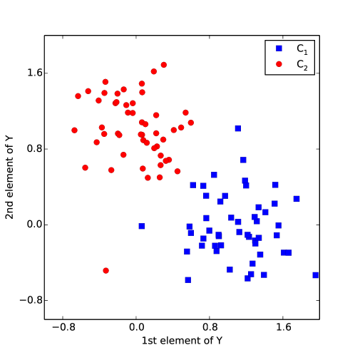
In this subsection, we apply the three classifiers defined in §4.1 to a binary classification problem using computer-simulated data sets, where and . In the first step, we independently generate 100 sets of training samples with each training sample being , where and if , and if , , , and . Here, and are sampled i.i.d. from and , respectively. Individual -values of one of the training samples are plotted in Figure 1.
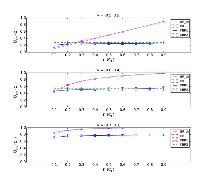
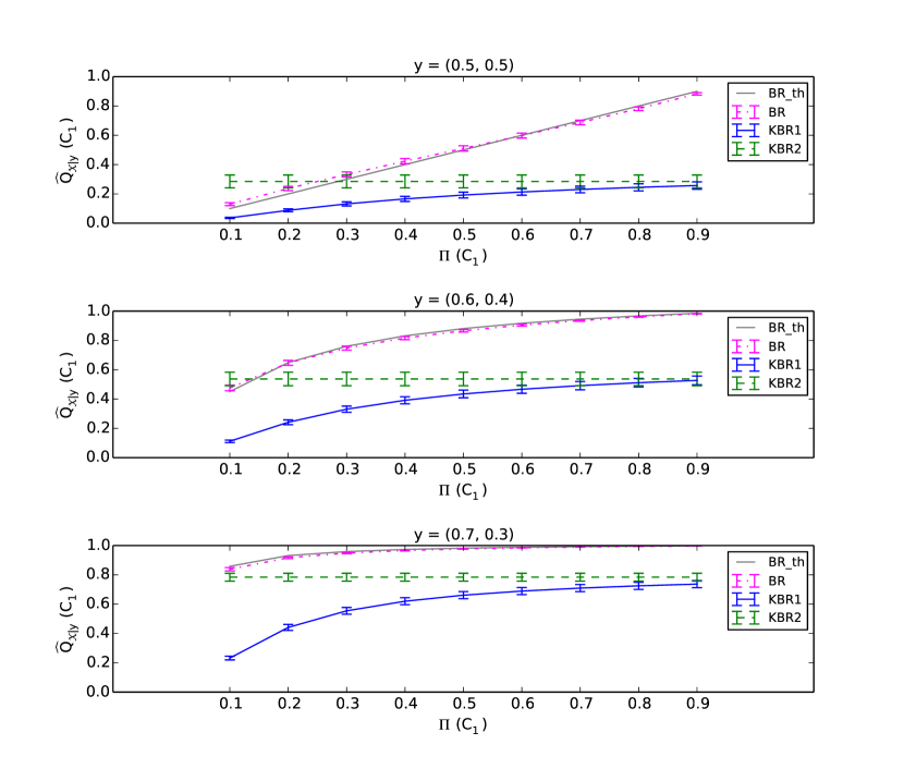
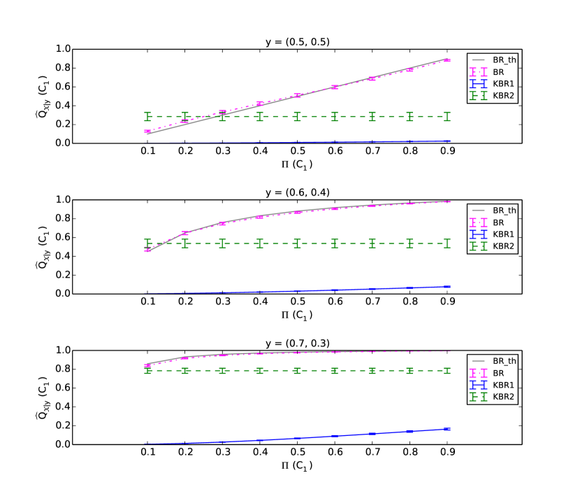
With each of the 100 training samples and a simulated prior probability of , or , the classifiers defined in §4.1 estimate the posterior probability of given a test value , that is, . Figures 2-5 show the mean (plus or minus standard error of the mean, SEM) of the 100 values of calculated by each of the classifiers, BR, KBR1, and KBR2. Here we show the case where in KBR1 and KBR2 is fixed to , and the regularization parameters of KBR1 are set to be (Figure 2), (Figure 3), (Figure 4), and (Figure 5). In Figures 2-5, BR_th illustrates the theoretical result of BR, where , , , and in BR are set to be , , , and , respectively.
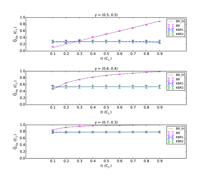
Consistent to §3.1, calculated by KBR1 is poorly influenced by compared with that by BR when and are set to be small (see Figures 2 and 3). In addition, calculated by KBR2 also seems to be uninfluenced by . When and are set to be larger, the effect of on becomes apparent in KBR1, however, the value of becomes too small (see Figures 4 and 5). These results suggest that in kernel Bayes’ rule, the posterior does not depend on the prior if and are negligible, which might be a contradiction to the nature of Bayes’ theorem. Moreover, even though the prior affects the posterior when and become larger, the posterior seems too much dependent on and , which are initially defined just for the regularization of matrices.
We have also tested all possible combinations of the following values for the parameters in KBR1 and/or KBR2: , , and . All the experimental results have been evaluated in a similar manner as above, and none of the results are found to be reasonable in the context of Bayesian inference.
§5 Conclusions
One of the important features of Bayesian inference is that it provides a reasonable way of updating the probability for a hypothesis as additional evidence is acquired. Kernel Bayes’ rule has been expected to enable Bayesian inference in RKHS. In other words, the posterior kernel mean has been considered to be reasonably estimated by kernel Bayes’ rule, given kernel mean expressions of the prior and likelihood. What is “reasonable” depends on circumstances, however, some of the results in this paper seem to show obviously unreasonable aspects of kernel Bayes’ rule, at least in the context of Bayesian inference.
First, as shown in §3.1, when and are non-singular matrices and so we set , the posterior kernel mean is entirely unaffected by the prior distribution on . This means that, in Bayesian inference with kernel Bayes’ rule, prior beliefs are in some cases completely neglected in calculating the kernel mean of the posterior distribution. Numerical evidence is also presented in §4.2. When the regularization parameters and are set to be small, the posterior probability calculated by kernel Bayes’ rule (KBR1) is almost unaffected by the prior probability in comparison with that by conventional Bayes’ rule (BR). Consistently, when the regularized inverse matrices in KBR1 are replaced for the Moore-Penrose generalized inverse matrices (KBR2), the posterior probability is also uninfluenced by the prior probability, which seems to be unsuitable in the context of Bayesian updating of a probability distribution.
Second, as discussed in §3.2 and §4.2, the posterior estimated by kernel Bayes’ rule considerably depends upon the regularization parameters and , which are originally introduced just for the regularization of matrices. A cross-validation approach is proposed in [2] to search for the optimal values of the parameters. However, theoretical foundations seem to be insufficient for the correct tuning of the parameters. Furthermore, in our experimental settings, we are not able to obtain a reasonable result using any combination of the parameter values, suggesting the possibility that there are no appropriate values for the parameters in general. Thus, we consider it difficult to solve the problem that and are not surjective by just adding regularization parameters.
§6 Appendix
§6.1 Estimation of and
Here we give the proof of Proposition 2.8.
Proof.
Let , , and denote the estimates of , , and , respectively. We define the estimates of and as
and put . According to Equations (5), for any and ,
where represents the empirical expectation operator. Thus, from Remark 2.6,
| (11) |
Similarly, for any ,
Thus, from Remark 2.6,
| (12) |
Next, we will derive . Since is a self-adjoint operator,
for any . On the other hand, from Equations (1),
for any . Hence, we have
| (13) |
for any . Replacing in Equation (13) for , we have
| (14) |
Using Equation (6), the left hand side of Equation (14) is given by
Therefore, we have
Replacing for , Equations (11) and (12) become
respectively.∎
§6.2 Non-singularity of and
Here we show that the assumption in §3.1 holds under reasonable conditions.
Definition 6.1.
Let be a real-valued function defined on a non-empty open domain . We say that is analytic if can be described by a Taylor expansion on a neighborhood of each point of .
Proposition 6.2.
Let be a positive definite kernel on . Let be a probability measure on which is absolutely continuous with respect to Lebesgue measure. Assume that is an analytic function on and that the RKHS corresponding to is infinite dimensional. Then for any i.i.d. random variables with the same distribution , the Gram matrix is non-singular almost surely with respect to .
Proof.
Let us put . Since the RKHS corresponding to is infinite dimensional, there are such that are linearly independent. Then and hence is a non-zero analytic function. Note that any non-trivial subvarieties of the euclidean spaces defined by analytic functions have Lebesgue measure zero. By this fact, the subvariety
has Lebesgue measure zero. Since is absolutely continuous, . This completes the proof. ∎
From Proposition 6.2, we easily obtain the following corollary.
Corollary 6.3.
Let be a Gaussian kernel on and let be i.i.d. random variables with the same normal distribution on . Then the Gram matrix is non-singular almost surely.
Proposition 6.4.
Let be a positive definite kernel on , a probability measure on which is absolutely continuous with respect to Lebesgue measure. Assume that is an analytic function on and that the RKHS corresponding to is infinite dimensional. Then for any except Lebesgue measure zero, and for any i.i.d. random variables with the same distribution , each for is non-zero almost surely, where , , and . Here denotes the set of positive real numbers.
Proof.
Let us put , , and
for and . We can verify that is non-singular almost everywhere on in the same way as in the proof of Proposition 6.2. Let us define a closed measure-zero set . Then is defined on for each . Using Cramer’s rule,
where stands for the -th column vector of . Here we denote by the numerator of , that is, . Let us choose such that are linearly independent in . It is easy to see that is a non-zero analytic function of on . Indeed, if , , , and , then . Hence is a closed subset of with Lebesgue measure zero for each . Thus, since is a non-zero analytic function of on for any ,
is a closed subset of with Lebesgue measure zero for each . Therefore is non-zero almost surely on for any because the subset is contained in for each . This completes the proof. ∎
The following corollary directly follows from Proposition 6.4.
Corollary 6.5.
Let be a Gaussian kernel on and let be i.i.d. random variables with the same normal distribution on . All other notations are as in Proposition 6.4. Then is non-singular almost surely for any except for those in a set of Lebesgue measure zero.
§6.3 Non-surjectivity of and
The covariance operators and are not surjective in general. This can be verified by the fact that they are compact operators. (If the operators are surjective on the corresponding RKHS which is infinite-dimensional, then they cannot be compact because of the open mapping theorem.) Here we present some easy examples where and are not surjective. Let us consider for simplicity the case . Let be a random variable on with a normal distribution . We prove that is not surjective under the usual assumption that the positive definite kernel on is Gaussian. In order to demonstrate this, we use the symbols defined in §3.3 and several proven results on function spaces and Fourier transforms (see [7], for example). Note that the following three propositions are introduced without proofs.
Proposition 6.6.
Let us put for , where . Then
Proposition 6.7.
For , almost everywhere. In particular, if , then almost everywhere.
Proposition 6.8.
For , put . Then .
Definition 6.9.
Let denote the density function of the normal distribution on , that is,
Let be a random variable on with . The linear operator is defined by for any , which is also described as
for any .
Proposition 6.10.
If , then
Proposition 6.11.
If , then .
Here, we denote by , , and the real part of a complex number, the imaginary part of a complex number, and the closure operator, respectively.
Corollary 6.12.
If , then .
Proof.
Remark 6.13.
If , then there uniquely exist such that by Corollary 6.12. This means that , where denotes the direct sum.
Proposition 6.14.
For any and for any , there exists such that . In other words, is dense in .
Proof.
Let denote the space of continuous complex-valued functions with compact support on . Let us define by
Note that coincides with the image of by the Fourier transform. Then, and . Hence . In other words, for any and for any , there exists such that because , which implies that there exists such that . This completes the proof. ∎
The following corollary has also been shown in Theorem 4.63 in [8].
Corollary 6.15.
.
Proof.
Definition 6.16.
Let us define as
where and denote the indicator functions of the intervals and , respectively. We also put and . Note that , because
Proposition 6.17.
.
Proof.
It is obvious that . Since , we see that
where . Hence . On the other hand,
Therefore .∎
Let us define for . Now, we prove that for any . This implies that is not surjective.
Proposition 6.18.
For any , .
Proof.
Suppose that there exists such that . Then, for any ,
| (15) |
Let us put . From Proposition 6.6, . Then, using Equation (10) and Proposition 6.8, the left hand side of Equation (15) equals
The right hand side of Equation (15) is equal to
Thus, Equation (15) is equivalent to the following equation:
| (16) |
Let us define and . Then . It is easy to see that as . Hence in . Since by Proposition 6.8, we have
which indicates that . Substituting for , Equation (16) becomes
| (17) |
If goes to infinity, the left hand side of Equation (17) becomes . On the other hand, the right hand side of Equation (17) becomes
This is a contradiction. Therefore, there exists no such that . This completes the proof. ∎
§7 Disclosures
The second author was partially supported by JSPS KAKENHI Grant Numbers 23540044, 15K04814. The authors declare no other conflicts of interest.
References
- [1] Le Song, Jonathan Huang, Alex Smola, Kenji Fukumizu. Hilbert space embeddings of conditional distributions with applications to dynamical systems. In Proceedings of the 26th Annual International Conference on Machine Learning, pages 961-968, 2009.
- [2] Kenji Fukumizu, Le Song, Arthur Gretton. Kernel Bayes’ rule: Bayesian inference with positive definite kernels. Journal of Machine Learning Research, 14:3753-3783, 2013.
- [3] Le Song, Kenji Fukumizu, Arthur Gretton. Kernel embeddings of conditional distributions. IEEE Signal Processing Magazine, 30:98-111, 2014.
- [4] Motonobu Kanagawa, Yu Nishiyama, Arthur Gretton, Kenji Fukumizu. Monte Carlo filtering using kernel embedding of distributions. In Proceedings of the Twenty-Eighth AAAI Conference on Artificial Intelligence, pages 1897-1903, 2014.
- [5] Kenji Fukumizu. Introduction to kernel methods (in Japanese). Asakura Shoten, Tokyo, 2010.
- [6] Roger A. Horn, Charles R Johnson. Matrix analysis, second edition. Cambridge University Press, Cambridge, 2013.
- [7] Walter Rudin. Real and complex analysis, third edition. McGraw-Hill Book Co., New York, 1987.
- [8] Ingo Steinwart, Andreas Christmann. Support vector machines. Information Science and Statistics. Springer, New York, 2008.