On the zeros of random harmonic polynomials: the truncated model

Abstract.

Motivated by Wilmshurst’s conjecture and more recent work of W. Li and A. Wei [17], we determine asymptotics for the number of zeros of random harmonic polynomials sampled from the truncated model, recently proposed by J. Hauenstein, D. Mehta, and the authors [10]. Our results confirm (and sharpen) their $(3/2)-$powerlaw conjecture [10] that had been formulated on the basis of computer experiments; this outcome is in contrast with that of the model studied in [17]. For the truncated model we also observe a phase-transition in the complex plane for the Kac-Rice density.

1. Introduction

A harmonic polynomial is a complex-valued harmonic function given by:

(1) $$F(z)=p(z)+\overline{q(z)},$$

where $p$ and $q$ are polynomials of degree $n$ and $m$ (respectively). Let $N_{F}$ denote the number of zeros of $F$, that is, points $z\in\mathbb{C}$ such that $F(z)=0$.

For $n>m$, we have the following bounds:

$$n\leq N_{F}\leq n^{2}.$$

The lower bound is based on the generalized argument principle and is sharp for each $m$ and $n$. The upper bound follows from applying Bezout’s theorem to the real and imaginary parts of $F(z)=0$ after noticing that the zeros are isolated, which was shown by Wilmshurst [29].

1.1. Wilmshurst’s conjecture

Wilmshurst made the conjecture that the Bezout bound can be improved to a function that is linear in $n$ for each fixed $m$, namely:

(2) $$N_{F}\leq 3n-2+m(m-1)\qquad\textrm{(Wilmshurst's conjecture)}$$

This conjecture is stated in [29, Remark 2] (see also [25] and [4]).

For $m=n-1$, the upper bound follows from Wilmshurst’s theorem [29], and examples were also given in [29] showing that this bound is sharp (shown independently in [2]). For $m=1$, the upper bound was shown by Khavinson and Swiatek [14] using anti-holomorphic dynamics. A proof of the Crofoot-Sarason conjecture given in [8] (cf. [3]) established that this bound is sharp. Counterexamples to the case $m=n-3$ were established analytically in [15], and counterexamples for a broad range of (finitely many) $m$ and $n$ were established in [10] using certified numerics. On the other hand, we still expect, in the spirit of (2), that $N_{F}$ satisfies an upper bound that is linear in $n$ for $m$ fixed; for instance, with S-Y. Lee, the authors conjectured in [15, Introduction] that $N_{F}\leq 2m(n-1)+n$.

1.2. A probabilistic version of the problem

Given the high variability of the number of zeros $N_{F}$, it is natural to ask the following.

Question 1.

What is the expectation $\mathbb{E}N_{F}$ of the number of zeros of a random harmonic polynomial?

This question was asked and answered by W. Li and A. Wei in [17], in the case when $p$ and $q$ are independently sampled from the complex Kostlan ensemble:

(3) $$p(z)=\sum_{k=0}^{n}a_{k}z^{k},\quad q(z)=\sum_{k=0}^{m}b_{k}z^{k},$$

where $a_{k}$ and $b_{k}$ are independent centered complex Gaussians with $\mathbb{E}a_{j}\overline{a_{k}}=\delta_{jk}\binom{n}{j}$ and $\mathbb{E}b_{j}\overline{b_{k}}=\delta_{jk}\binom{m}{k}$.

The choices of $p$ and $q$ in (3) lead to the following asymptotics (as $n\rightarrow\infty$):

(4) $$\mathbb{E}N_{F}\sim\left\{\begin{array}[]{cc}\frac{\pi}{4}n^{3/2},\quad\text{when }m=n,\\ n,\quad\text{when }m=\alpha n+o(n)\text{ with }0<\alpha<1,\end{array}\right.$$

Notice that when $m=\alpha n$ the average number of zeros is asymptotically the fewest possible. This seems to suggest that, on average, an even stronger form of Wilmshurst’s conjecture (2) holds. However, caution is needed here, and the dichotomy in (4) dissolves after choosing a definition of “random” in which the coefficients of $p$ and $q$ are more comparable in modulus (see Theorem 1 below).

In the model (3), where the coefficients of $p$ are asymptotically much larger in modulus than $q$ when $m=\alpha n$, $F$ tends to resemble an analytic polynomial and asymptotically obeys the fundamental theorem of algebra. In order to make $q$ more comparable to $p$, an alternative model (referred to as the “truncated model”) was proposed in [10] where the variances $\binom{m}{k}$ were replaced by $\binom{n}{k}$ in the definition (3) of $q$, while still choosing $m$ as the upper limit in the summation (see definition (5) below). For the truncated model, computer experiments performed in [10] led to a conjecture that the expectation $\mathbb{E}N_{F}$ has a $(3/2)-$powerlaw growth whenever $m=\alpha n$ for all $0<\alpha<1$. Here, we prove (and sharpen) this conjecture, see Theorem 1 below.

Note that we do not consider here the case $m=0$ of random complex analytic polynomials, where we would have $N_{F}=n$ almost surely (by the fundamental theorem of algebra). Yet, it is still interesting in that case to study the location of zeros; we refer the reader to Edelman and Kostlan’s paper [7, Sec. 8] and to the recent work of Zeitouni and Zelditch [30] establishing a large deviation principle for the location of the zeros of a random analytic polynomial.

1.3. Asymptotics for the truncated model

We revisit Question 1 while sampling $F(z)=p(z)+\overline{q(z)}$ randomly from the truncated model, i.e.,

(5) $$p(z)=\sum_{k=0}^{n}a_{k}z^{k},\quad q(z)=\sum_{k=0}^{m}b_{k}z^{k},$$

where $a_{k}$ and $b_{k}$ are independent centered complex Gaussians with $\mathbb{E}a_{j}\overline{a_{k}}=\delta_{jk}\binom{n}{j}$ and $\mathbb{E}b_{j}\overline{b_{k}}=\delta_{jk}\binom{n}{k}$.

Theorem 1.

Let $F(z)=p_{n}(z)+\overline{q_{m}(z)}$ be a random polynomial from the truncated model. For $m=\alpha n$ with $0<\alpha<1$, the expectation $\mathbb{E}N_{F}$ of the number of zeros of $F(z)$ satisfies the following asymptotic (as $n\rightarrow\infty$)

$$\mathbb{E}N_{F}\sim c_{\alpha}n^{3/2},$$

where $c_{\alpha}$ is given by

(6) $$c_{\alpha}=\frac{1}{2}\left(\arctan\left(\sqrt{\frac{\alpha}{1-\alpha}}\right)-\sqrt{\alpha(1-\alpha)}\right).$$

On the other hand, when $n\rightarrow\infty$ with $m$ fixed we have $\mathbb{E}N_{F}\sim n$.

Our methods can be used to describe asymptotics for the Kac-Rice density (providing the expected number of zeros over a prescribed region). We notice a phase-transition in this pointwise asymptotic, and the leading contribution $c_{\alpha}n^{3/2}$ is completely accounted for by zeros that are located within a critical distance from the origin, see Section 3.3.

Note that as $\alpha\rightarrow 1$, $c_{\alpha}\rightarrow\pi/4$, in agreement with [17, Thm. 1.1].

An interesting aspect of harmonic polynomials is that, unlike analytic polynomials, the function $F(z)=p(z)+\overline{q(z)}$ can reverse orientation. The orientation of $F$ can be determined by the sign of the Jacobian determinant $J_{F}(z)=|p^{\prime}(z)|^{2}-|q^{\prime}(z)|^{2}$. Let $N_{+}$ denote the number of zeros for which $F$ is orientation-preserving (i.e., $J_{F}<0$) and $N_{-}$ denote the number of zeros where $F$ is orientation-reversing ($J_{F}>0$).

Using a standard application of the generalized argument principle, we then notice the following corollary of Theorem 1, showing that orientation-reversing zeros are asymptotically as common as orientation-preserving ones.

Corollary 2.

For $m=\alpha n$ with $0<\alpha<1$, we have $\mathbb{E}N_{+}\sim\mathbb{E}N_{-}\sim\frac{c_{\alpha}}{2}n^{3/2}$.

Proof.

Almost surely we have $N_{F}=N_{+}+N_{-}$ (the presence of singular zeros is a probability zero event). By topological degree theory (or the generalized argument principle [5]) the difference $N_{+}-N_{-}$ is given by the winding number of $F$ along a sufficiently large circle. Moreover, since the $z^{n}$ term dominates, the winding number is $n$, and so we have $N_{+}=N_{-}+n$. Theorem 1 then implies that $\mathbb{E}N_{+}\sim\mathbb{E}N_{-}\sim\frac{c_{\alpha}}{2}n^{3/2}$. ∎

The coexistence of many zeros of opposite orientation suggests that the Jacobian of $F$ changes sign wildly throughout the complex plane (or otherwise that there is a high level of “condensation” of zeros into regions of common orientation). Taking this point into consideration, we conclude the introduction by posing the problem of investigating the topology of the orientation-reversing set $\Omega_{-}:=\{z\in\mathbb{C}:|p^{\prime}(z)|<|q^{\prime}(z)|\}$. It follows from applying the maximum principle to the harmonic function $\log|p^{\prime}(z)|-\log|q^{\prime}(z)|$ that each connected component of $\Omega_{-}$ contains at least one critical point of $p$. This implies that $\Omega_{-}$ has at most $n-1$ connected components. What can be said about the average number of components of $\Omega_{-}$?

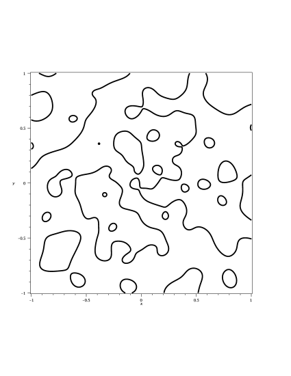
Figure 1. A portion of a random critical lemniscate (the critical set of a random harmonic polynomial) with $m=n=100$. Plotted in the region $\{z\in\mathbb{C}:|\Re z|<1,|\Im z|<1\}$. For $m=n$ the truncated model coincides with the Li-Wei model.

The critical set (the boundary of $\Omega_{-}$) is depicted in figure 1 for a random sample with $m=n=100$. Note that the critical set is a random rational lemniscate,

(7) $$\left\{z\in\mathbb{C}:\left|\frac{p^{\prime}(z)}{q^{\prime}(z)}\right|=1\right\},$$

similar to the random lemniscates studied recently by the authors [16]; the only difference is that in the model studied in [16, Sec. 1.2], the numerator $p$ and denominator $q$ of the rational function appear without differentiation. Based on the results in [16] we conjecture that when $m=n\rightarrow\infty$ the average number of connected components of the random critical lemniscate (7) grows linearly (the maximum rate possible).

1.4. Outline

In Section 2, we provide an exact formula for the average number of zeros for the truncated model. This is derived from a slight modification of [17]. The asymptotics stated in Theorem 1 are proved in Section 3. The proof uses the dominated convergence theorem after factoring out $n^{3/2}$. Establishing a dominating function requires several elementary estimates, and determining the pointwise limit of the integrand requires asymptotics for a truncated binomial sum. Such asymptotics are provided in Lemma 4, and the proof of Lemma 4 is given in the separate Section 4. The proof uses both forms of Laplace’s asymptotic method [19, Sec. 3.3, 3.4]: namely the case of an interior maximum (saddle-point) as well as the case of an end-point maximum. The presence of both cases is responsible for the phase-transition in the Kac-Rice density mentioned above (see also Section 3.3).

Acknowledgement. We wish to thank Seung-Yeop Lee for inspiring discussions and insightful suggestions and the anonymous referees for their helpful remarks.

2. An exact formula for $\mathbb{E}N_{f}$

Let $P_{m,n}(x):=\sum_{k=0}^{m}\binom{n}{k}x^{k}$ denote the binomial expansion of $(1+x)^{n}$ truncated at degree $m$.

Theorem 3.

The expectation $\mathbb{E}N_{F}(T)$ of the number of zeros of $F_{n,m}(z)=p_{n}(z)+\overline{q_{m}(z)}$ on a domain $T\subset\mathbb{C}$ is given by:

(8) $$\mathbb{E}N_{F}(T)=\frac{1}{\pi}\int_{T}\frac{1}{|z|^{2}}\frac{R_{1}^{2}+R_{2}^{2}-2R_{12}^{2}}{R_{3}^{2}\sqrt{(R_{1}+R_{2})^{2}-4R_{12}^{2}}}dA(z),$$

where $dA(z)$ denotes the Lebesgue measure on the plane, and

$$R_{12} =n^{2}|z|^{4}(1+|z|^{2})^{n-1}P_{m-1,n-1}(|z|^{2}),$$

$$R_{3} =(1+|z|^{2})^{n}+P_{m,n}(|z|^{2}),$$

$$R_{1} =R_{3}(n^{2}|z|^{4}+n|z|^{2})(1+|z|^{2})^{n-2}-n^{2}|z|^{4}(1+|z|^{2})^{2n-2},$$

$$R_{2} =R_{3}[n^{2}|z|^{4}P_{m-2,n-2}(|z|^{2})+n|z|^{2}P_{m-1,n-2}(|z|^{2})]-n^{2}|z|^{4}[P_{m-1,n-1}(|z|^{2})]^{2}.$$

Note: The analogous statements contained in [17, Thm. 1.1, Thm. 4.1] contain a little ambiguity. In fact the authors use the Kac-Rice formula for the harmonic function already in polar coordinates, thus viewing it as a random field defined over $[0,2\pi)\times(0,\infty)$ and with values in $\mathbb{R}^{2}$. In particular [17, Equation (1.1)] should either be modified with $|z|^{2}$ instead of $|z|$ (and $d\sigma(z)$ is still the Lebesgue measure on the complex plane) or the integration should be performed over the image of $T\subset\mathbb{C}$ under the polar change of coordinates (and in this case $|z|=\rho$). In other words, denoting by $\psi:\mathbb{C}\backslash\{0\}\to(0,2\pi)\times(0,\infty)$ the polar change of coordinates, the right expression for [17, Equation (1.1)] is:

(9) $$\frac{1}{\pi}\int_{T}\frac{1}{|z|^{2}}\frac{r_{1}^{2}+r_{2}^{2}-2r_{12}^{2}}{r_{3}^{2}\sqrt{(r_{1}+r_{2})^{2}-4r_{12}^{2}}}d\sigma(z)=\frac{1}{\pi}\int_{\psi(T)}\frac{1}{\rho^{2}}\frac{r_{1}^{2}+r_{2}^{2}-2r_{12}^{2}}{r_{3}^{2}\sqrt{(r_{1}+r_{2})^{2}-4r_{12}^{2}}}\rho d\rho d\theta$$

This ambiguity is no longer present in their asymptotic analysis.

Proof.

We follow closely the lines of the proof given in [17, Thm. 1.1, Thm. 4.1], adjusting certain computations as needed. Also, we simplify the first part of their proof by not switching to polar coordinates while obtaining equations (11) and (12) below.

Applying the Kac-Rice formula (restated in [17, Lemma 2.1]), we have:

(10) $$\mathbb{E}N_{F}(T)=\int_{T}\mathbb{E}\left(|\det J_{F}(z)|\big{|}F(z)=0\right)p(0;z)dA(z),$$

where, for each $z$, $p(s;z)$ is the probability density function of the random variable $s=F(z)$.

The modulus of the Jacobian determinant of $F(z)=p(z)+\overline{q(z)}$ is given by (see [6, Sec. 1.2])

(11) $$|J_{F}(z)|=\left||p^{\prime}(z)|^{2}-|q^{\prime}(z)|^{2}\right|=\frac{1}{|z|^{2}}\left||zp^{\prime}(z)|^{2}-|zq^{\prime}(z)|^{2}\right|,$$

and hence we have

(12) $$\mathbb{E}\left(|\det J_{F}(z)|\big{|}F(z)=0\right)=\frac{1}{|z|^{2}}\mathbb{E}\left(|u_{1}^{2}-u_{2}^{2}+v_{1}^{2}-v_{2}^{2}|\big{|}u_{3}=0,v_{3}=0\right),$$

where, for $j=1,2,3$, the expressions $u_{j},v_{j}$ are given by

$$u_{1} =\Re\sum_{k=0}^{n}ka_{k}z^{k},\quad v_{1}=\Im\sum_{k=0}^{n}ka_{k}z^{k},$$

$$u_{2} =\Re\sum_{k=0}^{m}kb_{k}z^{k},\quad v_{2}=\Im\sum_{k=0}^{m}kb_{k}z^{k},$$

$$u_{3} =\Re\left(p_{n}(z)+\overline{q_{m}(z)}\right),\quad v_{3}=\Im\left(p_{n}(z)+\overline{q_{m}(z)}\right).$$

Then letting $(U_{1},U_{2},V_{1},V_{2})$ denote the Gaussian vector that has the distribution of $(u_{1},u_{2},v_{1},v_{2})$ under the (linear) condition $u_{3}=0,v_{3}=0$, we have

(13) $$\mathbb{E}\left(|u_{1}^{2}-u_{2}^{2}+v_{1}^{2}-v_{2}^{2}|\big{|}u_{3}=0,v_{3}=0\right)=\mathbb{E}\left(|U_{1}^{2}-U_{2}^{2}+V_{1}^{2}-V_{2}^{2}|\right).$$

The covariance matrix $R$ of $(U_{1},U_{2},V_{1},V_{2})$ is given by [26, p. 30]

(14) $$R=C-BA^{-1}B^{T},$$

where

$$A_{2\times 2} =\text{cov}(u_{3},v_{3}),$$

$$B_{4\times 2} =\text{cov}((u_{1},u_{2},v_{1},v_{2}),(u_{3},v_{3})),$$

$$C_{4\times 4} =\text{cov}(u_{1},u_{2},v_{1},v_{2}).$$

First we compute

$$\mathbb{E}u_{3}^{2}=\mathbb{E}v_{3}^{2} =\frac{1}{2}\sum_{k=0}^{n}\binom{n}{k}|z|^{2k}+\frac{1}{2}\sum_{k=0}^{m}\binom{n}{k}|z|^{2k}=\frac{1}{2}(1+|z|^{2})^{n}+\frac{1}{2}P_{m,n}(|z|^{2}),$$

$$\mathbb{E}u_{1}u_{3}=\mathbb{E}v_{1}v_{3} =\frac{1}{2}\sum_{k=0}^{n}k\binom{n}{k}|z|^{2k}=\frac{1}{2}n|z|^{2}(1+|z|^{2})^{n-1},$$

$$\mathbb{E}u_{1}^{2}=\mathbb{E}v_{1}^{2} =\frac{1}{2}\sum_{k=0}^{n}k^{2}\binom{n}{k}|z|^{2k}=\frac{1}{2}(n^{2}|z|^{4}+n|z|^{2})(1+|z|^{2})^{n-2},$$

$$\mathbb{E}u_{2}u_{3}=\mathbb{E}v_{2}v_{3} =\frac{1}{2}\sum_{k=0}^{m}k\binom{n}{k}|z|^{2k}=\frac{1}{2}n|z|^{2}P_{m-1,n-1}(|z|^{2}),$$

$$\mathbb{E}u_{2}^{2}=\mathbb{E}v_{2}^{2} =\frac{1}{2}\sum_{k=0}^{m}k^{2}\binom{n}{k}|z|^{2k}=\frac{1}{2}(n^{2}|z|^{4}+n|z|^{2})P_{m-2,n-2}(|z|^{2}),$$

and hence

$$A_{2\times 2} =\frac{(1+|z|^{2})^{n}+P_{m,n}(|z|^{2})}{2}\begin{pmatrix}1&0\\ 0&1\\ \end{pmatrix},$$

$$B_{4\times 2} =\frac{1}{2}\begin{pmatrix}n|z|^{2}(1+|z|^{2})^{n-1}&0\\ n|z|^{2}P_{m-1,n-1}(|z|^{2})&0\\ 0&n|z|^{2}(1+|z|^{2})^{n-1}\\ 0&n|z|^{2}P_{m-1,n-1}(|z|^{2})\\ \end{pmatrix},$$

$$C_{4\times 4} =\frac{1}{2}\text{diag}((n^{2}|z|^{2}+n)(1+|z|^{2})^{n-2},(n^{2}|z|^{2}+n)P_{m-2,n-2}(|z|^{2}),$$

$$\quad\quad\quad\quad\quad(n^{2}|z|^{2}+n)(1+|z|^{2})^{n-2},(n^{2}|z|^{2}+n)P_{m-2,n-2}(|z|^{2})).$$

From these we compute (14):

$$R_{4\times 4}=\frac{1}{2R_{3}}\begin{pmatrix}R_{1}&-R_{12}&0&0\\ -R_{12}&R_{2}&0&0\\ 0&0&R_{1}&-R_{12}\\ 0&0&-R_{12}&R_{2}\\ \end{pmatrix},$$

where

$$R_{12} =n^{2}|z|^{4}(1+|z|^{2})^{n-1}P_{m-1,n-1}(|z|^{2}),$$

$$R_{3} =(1+|z|^{2})^{n}+P_{m,n}(|z|^{2}),$$

$$R_{1} =R_{3}(n^{2}|z|^{4}+n|z|^{2})(1+|z|^{2})^{n-2}-n^{2}|z|^{4}(1+|z|^{2})^{2n-2},$$

$$R_{2} =R_{3}[n^{2}|z|^{4}P_{m-2,n-2}(|z|^{2})+n|z|^{2}P_{m-1,n-2}(|z|^{2})]-n^{2}|z|^{4}[P_{m-1,n-1}(|z|^{2})]^{2}.$$

Applying [17, Cor. 2.1], we obtain:

(15) $$\mathbb{E}\left|U_{1}^{2}-U_{2}^{2}+V_{1}^{2}-V_{2}^{2}\right|=\frac{1}{R_{3}}\frac{R_{1}^{2}+R_{2}^{2}-2R_{12}^{2}}{\sqrt{(R_{1}+R_{2})^{2}-4R_{12}^{2}}}.$$

For each fixed $z$, the complex Gaussian $s=F(z)$ has probability density function

$$p(s;z)=\frac{1}{\pi R_{3}}\exp\{-|s|^{2}/R_{3}\},$$

and in particular

$$p(0;z)=\frac{1}{\pi R_{3}}.$$

Applying this along with equations (12), (13), and (15) to the Kac-Rice formula (10) we obtain the desired result (8). ∎

3. Proof of Theorem 1

3.1. The case when $m=\alpha n$

Applying Theorem 3 with $N_{F}:=N_{F}(\mathbb{C})$, switching to polar coordinates $r=|z|$, $dA(z)=rdrd\theta$, and integrating out the angular variable $\theta$, we are left with:

$$\mathbb{E}N_{F}=2\int_{0}^{\infty}\frac{1}{r}\frac{a_{1}^{2}+a_{2}^{2}-2a_{12}^{2}}{a_{3}^{2}\sqrt{(a_{1}+a_{2})^{2}-4a_{12}^{2}}}dr,$$

where

$$a_{12}=n^{2}r^{4}(1+r^{2})^{n-1}P_{m-1,n-1}(r^{2}),$$

$$a_{3}=(1+r^{2})^{n}+P_{m,n}(r^{2}),$$

$$a_{1}=a_{3}(n^{2}r^{4}+nr^{2})(1+r^{2})^{n-2}-n^{2}r^{4}(1+r^{2})^{2n-2},$$

$$a_{2}=a_{3}[n^{2}r^{4}P_{m-2,n-2}(r^{2})+nr^{2}P_{m-1,n-2}(r^{2})]-n^{2}r^{4}[P_{m-1,n-1}(r^{2})]^{2}.$$

Factoring $(1+r^{2})^{4n-4}$ from the numerator and $(1+r^{2})^{4n-2}$ from the denominator, we have:

(16) $$\mathbb{E}N_{F}=2n^{3/2}\int_{0}^{\infty}\frac{1}{n^{1/2}r(1+r^{2})^{2}}\frac{b_{1}^{2}+b_{2}^{2}-2b_{12}^{2}}{b_{3}^{2}\sqrt{(b_{1}+b_{2})^{2}-4b_{12}^{2}}}dr,$$

where

$$b_{12}=nr^{4}\frac{P_{m-1,n-1}(r^{2})}{(1+r^{2})^{n-1}},$$

$$b_{3}=1+\frac{P_{m,n}(r^{2})}{(1+r^{2})^{n}},$$

$$b_{1}=b_{3}[nr^{4}+r^{2}]-nr^{4},$$

$$b_{2}=b_{3}\left[nr^{4}\frac{P_{m-2,n-2}(r^{2})}{(1+r^{2})^{n-2}}+r^{2}\frac{P_{m-1,n-2}(r^{2})}{(1+r^{2})^{n-2}}\right]-nr^{4}\left[\frac{P_{m-1,n-1}(r^{2})}{(1+r^{2})^{n-1}}\right]^{2}.$$

We will apply Lebesgue’s dominated convergence theorem to take the limit of the integral appearing in (16). The following claim implies that the sequence of integrands in (16) is bounded by a single integrable function.

Claim:

$$\frac{b_{1}^{2}+b_{2}^{2}-2b_{12}^{2}}{b_{3}^{2}\sqrt{(b_{1}+b_{2})^{2}-4b_{12}^{2}}}=O(\sqrt{n}r^{3}),\quad\text{ as }n\rightarrow\infty.$$

Proof of Claim.

First we note that $a_{1}a_{2}\geq a_{12}^{2}$. This is by the Cauchy-Schwarz inequality, since it follows from the proof of Theorem 3 that $a_{1}=\mathbb{E}U_{1}^{2},a_{2}=\mathbb{E}U_{2}^{2},$ and $a_{12}=\mathbb{E}U_{1}U_{2}$, where $U_{1}$ and $U_{2}$ are Gaussian random variables.

This implies that $b_{1}b_{2}\geq b_{12}^{2}$. Since $b_{3}\geq 1$, we have:

$$\frac{b_{1}^{2}+b_{2}^{2}-2b_{12}^{2}}{b_{3}^{2}\sqrt{(b_{1}+b_{2})^{2}-4b_{12}^{2}}} \leq\sqrt{b_{1}^{2}+b_{2}^{2}-2b_{12}^{2}}$$

$$=\sqrt{(b_{1}-b_{2})^{2}+2(b_{1}b_{2}-b_{12}^{2})}$$

$$\leq\sqrt{(b_{1}-b_{2})^{2}}+\sqrt{2(b_{1}b_{2}-b_{12}^{2})}$$

$$=|b_{1}-b_{2}|+\sqrt{2}\sqrt{b_{1}b_{2}-b_{12}^{2}}$$

Thus, it suffices to show that

(17) $$b_{1}-b_{2}=O(\sqrt{n}+r^{2}),$$

and

(18) $$b_{1}b_{2}-b_{12}^{2}=O(nr^{6}).$$

Let $q_{m,n}:=\frac{P_{m,n}(r^{2})}{(1+r^{2})^{n}}$. Then, $b_{3}=1+q_{m,n}$, and we have:

$$b_{1}=(1+q_{m,n})(nr^{4}+r^{2})-nr^{4},$$

and

$$b_{2}=(1+q_{m,n})\left(nr^{4}q_{m-2,n-2}+r^{2}q_{m-1,n-2}\right)-nr^{4}q_{m-1,n-1}^{2}.$$

These lead to:

$$b_{1}-b_{2}=nr^{4} \left((1+q_{m,n})(1-q_{m-2,n-2})-(1-q_{m-1,n-1}^{2})\right)$$

$$+(1+q_{m,n})r^{2}\left(1-q_{m-1,n-2}\right).$$

The term $(1+q_{m,n})r^{2}\left(1-q_{m-1,n-2}\right)$ is bounded by $2r^{2}$. We consider the remaining term $nr^{4}\left((1+q_{m,n})(1-q_{m-2,n-2})-(1-q_{m-1,n-1}^{2})\right)$ which can be rewritten as:

$$nr^{4}\left((1+q_{m,n})(q_{m-1,n-1}-q_{m-2,n-2})+(1-q_{m-1,n-1})(q_{m,n}-q_{m-1,n-1})\right)$$

$$\leq nr^{4}\left(2(q_{m-1,n-1}-q_{m-2,n-2})+(q_{m,n}-q_{m-1,n-1})\right)$$

$$= nr^{4}\left(2\binom{n-2}{m-1}\frac{r^{2(m-1)}}{(1+r^{2})^{n-1}}+\binom{n-1}{m}\frac{r^{2m}}{(1+r^{2})^{n}}\right)$$

$$\leq nr^{4}\left(2\binom{n-2}{m-1}+\binom{n-1}{m}\right)\frac{r^{2(m-1)}}{(1+r^{2})^{n-1}}$$

$$\leq 3n\binom{n-1}{m}\frac{r^{2(m+1)}}{(1+r^{2})^{n-1}},$$

where we have used the identity

(19) $$q_{m,n}-q_{m-1,n-1}=\binom{n-1}{m}\frac{r^{2m}}{(1+r^{2})^{n}},$$

which can be seen as follows

$$q_{m,n}-q_{m-1,n-1} =\frac{\sum_{k=0}^{m}\binom{n}{k}r^{2k}-(1+r^{2})\sum_{k=0}^{m-1}\binom{n-1}{k}r^{2k}}{(1+r^{2})^{n}}$$

$$=\frac{\sum_{k=1}^{m-1}\left(\binom{n}{k}-\binom{n-1}{k}-\binom{n-1}{k-1}\right)r^{2k}}{(1+r^{2})^{n}}+\binom{n-1}{m}\frac{r^{2m}}{(1+r^{2})^{n}}$$

$$=\binom{n-1}{m}\frac{r^{2m}}{(1+r^{2})^{n}}.$$

Applying the first derivative test to $\frac{x^{m+1}}{(1+x)^{n-1}}$ over the interval $x>0$ we find that the maximum occurs at $x=\frac{m+1}{n-m-2}$. Thus, we have:

$$3n\binom{n-1}{m}\frac{r^{2(m+1)}}{(1+r^{2})^{n-1}} \leq 3n\binom{n-1}{m}\frac{(\frac{m+1}{n-m-2})^{m+1}}{(\frac{n-1}{n-m-2})^{n-1}}$$

$$\leq 3n\binom{n-1}{m}\frac{(m+1)^{m+1}(n-m-2)^{n-m-2}}{(n-1)^{n-1}}$$

$$=3n\frac{m+1}{n-1-m}\binom{n-1}{m+1}\frac{(m+1)^{m+1}(n-m-2)^{n-m-2}}{(n-1)^{n-1}}$$

$$\leq Cn\frac{m+1}{n-1-m}\sqrt{\frac{n-1}{(m+1)(n-m-2)}}=O(n^{1/2}),$$

where we have used Stirling’s approximation while recalling that $m=\alpha n$.

This establishes (17).

Next we consider $b_{1}b_{2}-b_{12}^{2}$.

We have:

$$b_{1}b_{2}-b_{12}^{2}=n^{2}r^{8}\left(q_{m,n}\left[(1+q_{m,n})q_{m-2,n-2}-q_{m-1,n-1}^{2}\right]-q_{m-1,n-1}^{2}\right)$$

$$+(1+q_{m,n})r^{2}\left(b_{2}+\frac{P_{m-1,n-2}(r^{2})}{(1+r^{2})^{n-2}}q_{m,n}\right).$$

Part of this can be estimated as follows:

$$(1+q_{m,n})r^{2}\left(b_{2}+\frac{P_{m-1,n-2}(r^{2})}{(1+r^{2})^{n-2}}q_{m,n}\right)\leq 2r^{2}(2(nr^{4}+r^{2})+1)=O(nr^{6}).$$

Since $b_{1}b_{2}-b_{12}^{2}\geq 0$, in order to prove (18), it is enough to show that for the remaining terms we have:

$$n^{2}r^{8}\left(q_{m,n}\left[(1+q_{m,n})q_{m-2,n-2}-q_{m-1,n-1}^{2}\right]-q_{m-1,n-1}^{2}\right)\leq 0.$$

We notice that

$$\left(q_{m,n}\left[(1+q_{m,n})q_{m-2,n-2}-q_{m-1,n-1}^{2}\right]-q_{m-1,n-1}^{2}\right)$$

$$= \left(q_{m,n}(1+q_{m,n})q_{m-2,n-2}-(1+q_{m,n})q_{m-1,n-1}^{2}\right)$$

$$= \left(1+q_{m,n}\right)\left(q_{m,n}q_{m-2,n-2}-q_{m-1,n-1}^{2}\right).$$

We will show that $q_{m,n}q_{m-2,n-2}-q_{m-1,n-1}^{2}\leq 0$.

Using again the identity (19), we have:

$$q_{m,n}q_{m-2,n-2}-q_{m-1,n-1}^{2} =q_{m,n}\left(q_{m-1,n-1}-\binom{n-2}{m-1}\frac{r^{2(m-1)}}{(1+r^{2})^{n-1}}\right)-q_{m-1,n-1}^{2}$$

$$=q_{m-1,n-1}\left(q_{m,n}-q_{m-1,n-1}\right)-q_{m,n}\binom{n-2}{m-1}\frac{r^{2(m-1)}}{(1+r^{2})^{n-1}}$$

$$=q_{m-1,n-1}\binom{n-1}{m}\frac{r^{2m}}{(1+r^{2})^{n}}-q_{m,n}\binom{n-2}{m-1}\frac{r^{2(m-1)}}{(1+r^{2})^{n-1}}$$

$$=\frac{\binom{n-2}{m-1}r^{2(m-1)}}{(1+r^{2})^{2n-1}}\left[r^{2}\frac{n-1}{m}P_{m-1,n-1}(r^{2})-P_{m,n}(r^{2})\right].$$

Finally, we have:

$$r^{2}\frac{n-1}{m}P_{m-1,n-1}(r^{2})-P_{m,n}(r^{2})=-1+\sum_{j=1}^{m}\left(\frac{n-1}{m}\binom{n-1}{j-1}-\binom{n}{j}\right)r^{2j},$$

and we see that each coefficient $\frac{n-1}{m}\binom{n-1}{j-1}-\binom{n}{j}=\binom{n-1}{j-1}\left(\frac{n-1}{m}-\frac{n}{j}\right)$ is negative.

∎

Having justified an application of Lebesgue’s dominated convergence theorem, we find the pointwise limit of the integrand in (16) using the following asymptotic (whose proof is given in Section 4).

Lemma 4.

Let $x\geq 0$. For all $0<\alpha<1$, we have (as $n\rightarrow\infty$ with $m=\alpha n$):

$$\frac{P_{m,n}(x)}{(1+x)^{n}}=\left\{\begin{array}[]{cc}1+O(1/n),\quad 0\leq x<\frac{\alpha}{1-\alpha},\\ O(\exp\{-cn\}),\quad x>\frac{\alpha}{1-\alpha}.\\ \end{array}\right.$$

According to this asymptotic, for $r^{2}>\frac{\alpha}{1-\alpha}$, the integrand in Equation (16) converges to zero, and for $0<r^{2}<\frac{\alpha}{1-\alpha}$, we see that $b_{2}=b_{1}(1+O(1/n))$, and

$$\frac{b_{1}^{2}+b_{2}^{2}-2b_{12}^{2}}{n^{1/2}b_{3}^{2}\sqrt{(b_{1}+b_{2})^{2}-4b_{12}^{2}}}=\frac{\sqrt{b_{1}^{2}-b_{12}^{2}}}{n^{1/2}b_{3}^{2}}(1+O(1/n))\sim\frac{r^{3}}{2}.$$

Thus, we have

$$N_{F}\sim n^{3/2}\int_{0}^{\sqrt{\alpha/(1-\alpha)}}\frac{r^{2}}{(1+r^{2})^{2}}dr=n^{3/2}c_{\alpha},$$

where

$$c_{\alpha}=\int_{0}^{\sqrt{\alpha/(1-\alpha)}}\frac{r^{2}}{(1+r^{2})^{2}}dr.$$

In order to determine $c_{\alpha}$, we make the change of variable $r=\tan(\theta),dr=\sec^{2}(\theta)d\theta$:

$$\int_{0}^{\sqrt{\alpha/(1-\alpha)}}\frac{r^{2}}{(1+r^{2})^{2}}dr=\int_{0}^{A}\sin^{2}(\theta)d\theta,\quad A=\arctan\left(\sqrt{\frac{\alpha}{1-\alpha}}\right).$$

Thus, we have

$$c_{\alpha}=\frac{1}{2}\left(\arctan\left(\sqrt{\frac{\alpha}{1-\alpha}}\right)-\sqrt{\alpha(1-\alpha)}\right).$$

This completes the proof of Theorem 1 in the case that $m=\alpha n$ with $0<\alpha<1$.

3.2. The case when $n\rightarrow\infty$ with $m$ fixed

This case is simpler and does not require Lemma 4. Omitting the details, we find that $b_{2},b_{12}$, converge to zero, $b_{3}$ converges to $1$, and

$$N_{F}\sim 2n\int_{0}^{\infty}\frac{r}{(1+r^{2})^{2}}dr=n.$$

3.3. Asymptotics of the Kac-Rice density

Consider again the case when $m=\alpha n$, with $0<\alpha<1$. Above, we have factored out $n^{3/2}$ from the Kac-Rice density in order to apply the dominated convergence theorem, but Lemma 4 can also be used to find the pointwise asymptotic. The Kac-Rice density is asymptotic (as $n\rightarrow\infty$) to $\frac{n^{3/2}|z|}{2\pi(1+|z|^{2})^{2}}$ for $|z|<\sqrt{\alpha/(1-\alpha)}$, and it is asymptotic to $\frac{n}{\pi(1+|z|^{2})^{2}}$ for $|z|>\sqrt{\alpha/(1-\alpha)}$. Thus, the leading contribution of zeros are located within the distance $\sqrt{\alpha/(1-\alpha)}$ from the origin. This critical radius originates in the proof of Lemma 4 (based on Laplace’s method), see Cases 1 and 2 in Section 4.

4. Proof of Lemma 4 using Laplace’s method

The following formula is provided in [20, Lemma 1].

Lemma 5.

For $0<m<n-1$

(20) $$\frac{P_{m,n}(x)}{(1+x)^{n}}=\binom{n}{m}(n-m)\int_{x/(x+1)}^{1}u^{m}(1-u)^{n-m-1}du.$$

We apply Laplace’s method to derive Lemma 4 from Lemma 5. Rewriting the integrand, we have for $m=\alpha n$:

$$\int_{x/(x+1)}^{1}e^{nh(u)}g(u)du,$$

where $h(u)=[\alpha\log(u)+(1-\alpha)\log(1-u)]$, and $g(u)=(1-u)^{-1}$.

Case 1: When $x/(x+1)<\alpha$, $h(u)$ achieves its maximum at $u=\alpha$, the unique solution of the saddle-point equation:

$$h^{\prime}(u)=\alpha/u-(1-\alpha)/(1-u)=0.$$

Applying Laplace’s method [19, Sec. 3.4], we have:

$$\int_{x/(x+1)}^{1}e^{nh(u)}g(u)du =e^{nh(\alpha)}g(\alpha)\sqrt{\frac{2\pi}{-nh^{\prime\prime}(\alpha)}}\left(1+O(n^{-1})\right)$$

$$=\alpha^{\alpha n}(1-\alpha)^{(1-\alpha)n-1}\sqrt{\frac{2\pi\alpha(1-\alpha)}{n}}\left(1+O(n^{-1})\right).$$

Applying Stirling’s approximation, we have:

(21) $$\binom{n}{m}(n-m)=\frac{\sqrt{n}}{\alpha^{\alpha n}(1-\alpha)^{(1-\alpha)n-1}\sqrt{2\pi\alpha(1-\alpha)}}\left(1+O(n^{-1})\right).$$

Combining these results into (20), we find:

$$\frac{P_{m,n}(x)}{(1+x)^{n}}=\left(1+O(n^{-1})\right).$$

Case 2: When $x/(x+1)>\alpha$, the saddle-point $u=\alpha$ is outside of the interval of integration, and $h(u)$ instead achieves its maximum at the left end-point $u=x/(x+1)$. We thus have (by the alternative form of Laplace’s method [19, Sec. 3.3]):

$$\int_{x/(x+1)}^{1}e^{nh(u)}g(u)du =e^{nh(x/(x+1))}\frac{g(x/(x+1))}{-nh^{\prime}(x/(x+1))}\left(1+O(n^{-1})\right)$$

$$\sim\left(\frac{x}{x+1}\right)^{\alpha n+1}\left(\frac{1}{x+1}\right)^{(1-\alpha)n-1}\left(\frac{1}{n(x(1-\alpha)-\alpha)}\right).$$

Combining this with (21), we see that

$$\frac{P_{m,n}(x)}{(1+x)^{n}}\sim c_{1}(x,\alpha)\frac{e^{-c_{2}(x,\alpha)n}}{\sqrt{n}}.$$

5. Concluding remarks

We have shown that the average number of zeros of a random harmonic polynomial sampled from the truncated model has order $n^{3/2}$ when $m$ is a fixed fraction of $n$ and grows linearly in $n$ when $m$ is fixed. In comparison with the Li-Wei model [17, Thm. 1.1], this behavior seems more indicative of (a probabilistic version) of Wilmshurst’s conjecture.

Extending the above-mentioned breakthrough [14], Khavinson and Neumann [12] used anti-holomorphic dynamics to count zeros of rational harmonic functions of the form $r(z)+\bar{z}$, giving a complete solution to astronomer S-H. Rhie’s conjecture [24] in gravitational lensing. For further discussion and related results, see [13, 11, 1]. In order to model stochastic gravitational lensing, the zeros of random harmonic functions were studied by A. Wei in his thesis [27, Ch. 3] and by Petters, Rider, and Teguia [22, 23].

Is the variance of $N_{F}$ asymptotically proportional to the mean? Computer experiments in [10] suggest that the answer is (perhaps surprisingly, cf. [9]) “no”, and that the variance instead has order $n^{2}$.

References

- [1] P. M. Bleher, Y. Homma, L. L. Ji, R. K. W. Roeder, Counting zeros of harmonic rational functions and its application to gravitational lensing, Internat. Math. Res. Notices., 8 (2014), 2245-2264.
- [2] D. Bshouty, W. Hengartner, and T. Suez, The exact bound on the number of zeros of harmonic polynomials, J. Anal. Math., 67 (1995), 207-218.
- [3] D. Bshouty, A. Lyzzaik, On Crofoot-Sarason’s conjecture for harmonic polynomials, Comp. Meth. Funct. Thy., 4 (2004), 35-41.
- [4] D. Bshouty, A. Lyzzaik, Problems and conjectures for planar harmonic mappings: in the Proceedings of the ICM2010 Satellite Conference: International Workshop on Harmonic and Quasiconformal Mappings (HQM2010), Special issue in: J. Analysis, 18 (2010), 69-82.
- [5] P. Duren, W. Hengartner, R. S. Langesen, The argument principle for harmonic functions, Amer. Math. Monthly, 103 (1996), 411-415.
- [6] P. Duren, Harmonic Mappings in the Plane, Cambridge University Press, 2004.
- [7] A. Edelman and E. Kostlan, How many zeros of a random polynomial are real?, Bull. Amer. Math. Soc. 32 (1995), 1-37.
- [8] L. Geyer, Sharp bounds for the valence of certain harmonic polynomials, Proc. AMS, 136 (2008), 549-555.
- [9] A. Granville, I. Wigman, The distribution of the zeros of random trigonometric polynomials, Amer. J. Math., 133 (2011), 295-357.
- [10] J. Hauenstein, A. Lerario, E. Lundberg, D. Mehta, Experiments on the zeros of harmonic polynomials using certified counting, Exper. Math., 24 (2015), 133-141.
- [11] D. Khavinson, E. Lundberg, Transcendental harmonic mappings and gravitational lensing by isothermal galaxies, Complex Anal. Oper. Thy. 4 (2010), 515-524.
- [12] D. Khavinson, G. Neumann, On the number of zeros of certain rational harmonic functions, Proc. AMS, 134 (2006), 1077-1085.
- [13] D. Khavinson, G. Neumann, From the fundamental theorem of algebra to astrophysics: a harmonious path, Notices AMS, 55 (2008), 666-675.
- [14] D. Khavinson, G. Swiatek, On a maximal number of zeros of certain harmonic polynomials, Proc. AMS, 131 (2003), 409-414.
- [15] S-Y. Lee, A. Lerario, E. Lundberg, Remarks on Wilmshurst’s theorem, Indiana U. Math. J., 64 No. 4 (2015), 1153 1167
- [16] A. Lerario, E. Lundberg, On the geometry of random lemniscates, preprint.
- [17] W. V. Li, A. Wei, On the expected number of zeros of random harmonic polynomials, Proc. AMS, 137 (2009), 195-204.
- [18] D. S. Lubinsky, I. E. Pritsker, X. Xie, Expected number of real zeros for random linear combinations of orthogonal polynomials, preprint: http://arxiv.org/abs/1503.06376
- [19] P. Miller, Applied Asymptotic Analysis, Amer. Math. Soc., 2006.
- [20] I. V. Ostrovskii, On a problem of A. Eremenko, CMFT, 4 (2004), 275-282.
- [21] R. Peretz, J. Schmid, On the zero sets of certain complex polynomials, Proceedings of the Ashkelon Workshop on Complex Function Theory (1996), 203-208, Israel Math. Conf. Proc. 11, Bar-Ilan Univ. Ramat Gan, 1997.
- [22] A.O. Petters, B. Rider, A.M. Teguia, A mathematical theory of stochastic microlensing I: random time-delay functions and lensing maps, J. Math. Phys. 50 (2009), 072503.
- [23] A.O. Petters, B. Rider, A.M. Teguia, A mathematical theory of stochastic microlensing II: random images, shear, and the Kac-Rice Formula, J. Math. Phys. 50 (2009), 122501.
- [24] S. Rhie, n-point gravitational lenses with 5(n-1) images, archiv:astro-ph/0305166 (2003).
- [25] T. Sheil-Small, Complex Polynomials, Cambridge University Press, 2002.
- [26] Y.L. Tong, The multivariate normal distribution, Springer-Verlag, 1990.
- [27] A. Wei, Random harmonic functions and multivariate Gaussian estimates, D. Phil. thesis, Univ. of Delaware, 2009.
- [28] A. S. Wilmshurst, Complex harmonic polynomials and the valence of harmonic polynomials, D. Phil. thesis, Univ. of York, U.K., 1994.
- [29] A. S. Wilmshurst, The valence of harmonic polynomials, Proc. AMS 126 (1998), 2077-2081.
- [30] O. Zeitouni, S. Zelditch, Large deviations of empirical measures of zeros of random polynomials, IMRN, Vol. 2010, No. 20, 3935-3992.