Contraction method and Lambda-Lemma

Abstract

We reprove the $\lambda$-Lemma for finite dimensional gradient flows by generalizing the well-known contraction method proof of the local (un)stable manifold theorem. This only relies on the forward Cauchy problem. We obtain a rather quantitative description of (un)stable foliations which allows to equip each leaf with a copy of the flow on the central leaf – the local (un)stable manifold. These dynamical thickenings are key tools in our recent work [Web]. The present paper provides their construction.

1 Introduction and main results

Throughout $(M^{n},g)$ denotes a Riemannian manifold of finite dimension $n$ and $f$ is a function on $M$ of class $C^{r+1}$ with $r\geq 1$. We assume further that the downward gradient equation

$$\dot{u}(t):=\tfrac{d}{dt}u(t)=-(\nabla f)\circ u(t)$$ (1)

for curves $u:[0,\infty)\to M$ generates a complete forward flow $\varphi=\{\varphi_{t}\}_{t\geq 0}$. This holds true, for instance, whenever $f$ is exhaustive, that is whenever all sublevel sets $M^{a}=\{f\leq a\}$ are compact. By $x$ we denote throughout a non-degenerate critical point of $f$ of Morse index $k={\rm ind}(x)$ with $1\leq k\leq n-1$; for $k\in\{0,n\}$ there is no $\lambda$-Lemma. In the following we give an overview of the contents of this paper. Definitions and proofs are given in subsequent sections.

The $\lambda$-Lemma was proved by Palis [Pal67, Pal69] in the late 60’s. Its backward version asserts that, given a hyperbolic singularity $x$ of a $C^{1}$ vector field $X$ on a finite dimensional manifold, the corresponding backward flow applied to any disk $D$ transverse to the unstable manifold $W^{u}(x)$ converges in $C^{1}$ and locally near $x$ to the stable manifold of $x$; cf. [PdM82, Ch. 2 §7] and Figure 2. Since the $\lambda$-Lemma is a local result we pick convenient coordinates about $x$.

Definition 1.1 (Local coordinates and notation – Figure 1).

1. Associated to the Hessian operator $A=D(\nabla f)_{x}$ there is the spectral splitting $X:=T_{x}M=E^{-}\oplus E^{+}$ in (7) with spectral projections $\pi_{\pm}$ and where $E^{-/+}=T_{x}W^{u/s}(x)$. Consider the spectral gap $d>0$ of $A$, see (6), and fix a constant $\lambda\in(0,d)$ – which will become the rate of exponential decay. Consider the constants $0<\delta<\mu<d$ defined by Figure 5.

   

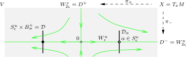
   Figure 1: Local coordinates near non-degenerate critical point

2. Express the downward gradient equation (1) via exponential coordinates in the form of the ODE (12) on a ball $B_{\rho_{0}}\subset X:=T_{x}M$ whose radius $\rho_{0}\leq 1$ satisfies (14). In these coordinates the origin represents $x$ and the local flow will be denoted by $\phi=\{\phi_{t}\}$. The non-linearity $h$ of this ODE, also shown in (12), satisfies the Lipschitz estimates of Lemma 2.5.

   Notation. The notation of coordinate representatives of global objects such as $W^{s}(x)\subset M$ will be the global notation without the $x$ such as $W^{s}$.

3. By Remark 3.9 we take our local model of the form $V=D^{-}\times D^{+}$ where $V\subset B_{\rho_{0}}$ and $D^{-/+}=W^{u/s}_{2\varsigma}\subset E^{\mp}$ represent a/de/scending disks, see (18) and Remark 3.6, whose parameter $2\varsigma$ is determined by the inclusions (25). In this local model the graph maps (20) and (23) of the local un/stable manifolds take on the rather simple form

   $${\mathcal{F}}^{\infty}=(id,0):D^{-}\to D^{-}\times D^{+},\qquad{\mathcal{G}}^{\infty}=(0,id):D^{+}\to D^{-}\times D^{+}.$$

4. Suppose ${\varepsilon}\in(0,\varsigma)$ and consider the descending sphere $S^{u}_{\varepsilon}={\partial}W^{u}_{\varepsilon}$ contained in $W^{u}_{2\varsigma}=D^{-}$. Pick a constant $\varkappa\in(0,1]$ such that the radius $\varkappa$ ball $B_{\varkappa}^{+}\subset E^{+}$ lies in the ascending disk $W^{s}_{\varsigma}\subset W^{s}_{2\varsigma}=D^{+}$. Consequently the hypersurface ${\mathcal{D}}:=S^{u}_{\varepsilon}\times B_{\varkappa}^{+}$ is contained in the interior of $V$. The fiber ${\mathcal{D}}_{\alpha}:=\{{\alpha}\}\times B_{\varkappa}^{+}$ over ${\alpha}\in S^{u}_{\varepsilon}$ is a translated ball of codimension $k$.

Theorem 1.2 (Backward $\lambda$-Lemma).

Given the local model on $V=W^{u}_{2\varsigma}\times W^{s}_{2\varsigma}\subset E^{-}\oplus E^{+}=T_{x}M$ provided by Definition 1.1 nearby a non-degenerate critical point $x$ of a function $f:M\to{\mathbb{R}}$, pick ${\varepsilon}\in(0,\varsigma)$. Then the following is true. There is a ball $B^{+}\subset E^{+}$ about the origin of some radius $\frac{\rho}{2}>0$, a constant $T_{0}>0$, and a Lipschitz continuous map

$$\begin{split}{\mathcal{G}}:[T_{0},\infty)\times S^{u}_{\varepsilon}\times B^{+}&\to V\subset E^{-}\oplus E^{+}\\ (T,{z_{-}},z_{+})&\mapsto\left(G^{T}_{z_{-}}(z_{+}),z_{+}\right)=:{\mathcal{G}}^{T}_{z_{-}}(z_{+})\end{split}$$

defined by (36) below which is of class $C^{r}$ in ${z_{-}}$ and $z_{+}$. It satisfies the identity ${\mathcal{G}}^{T}_{z_{-}}(0)=\phi_{-T}({z_{-}})$ and the graph of $G^{T}_{z_{-}}$ consists of those $z\in V$ which satisfy $\pi_{+}z\in B^{+}$ and reach the fiber ${\mathcal{D}}_{z_{-}}=\{{z_{-}}\}\times B^{+}_{\varkappa}$ at time $T$, that is

$$\begin{split}{\mathcal{G}}^{T}_{z_{-}}(B^{+})={\phi_{T}}^{-1}{\mathcal{D}}_{z_{-}}\cap\left(E^{-}\times B^{+}\right).\end{split}$$

Moreover, the graph map ${\mathcal{G}}^{T}_{z_{-}}$ converges uniformly in $C^{1}$, as $T\to\infty$, to the local stable manifold graph map ${\mathcal{G}}^{\infty}$ as illustrated by Figure 2. More precisely,

$$\begin{split}\bigl{\|}{\mathcal{G}}^{T}_{z_{-}}(z_{+})-{\mathcal{G}}^{\infty}(z_{+})\bigr{\|}=\bigl{\|}G^{T}_{z_{-}}(z_{+})\bigr{\|}&\leq e^{-T\frac{\lambda}{8}},\\ \bigl{\|}d{\mathcal{G}}^{T}_{z_{-}}(z_{+})v-d{\mathcal{G}}^{\infty}(z_{+})v\bigr{\|}=\bigl{\|}dG^{T}_{z_{-}}(z_{+})v\bigr{\|}&\leq c_{*}e^{-T\frac{\lambda}{8}}\left\|v\right\|,\end{split}$$ (2)

for all $T\geq T_{0}$, ${z_{-}}\in S^{u}_{\varepsilon}$, $z_{+}\in B^{+}$, and $v\in E^{+}$ where $c_{*}>0$ is a constant. Estimate two requires $f\in C^{2,1}$ near $x$ in which case $T\mapsto\frac{d}{dT}{\mathcal{G}}(T,z_{-},z_{+})$ is also Lipschitz continuous.

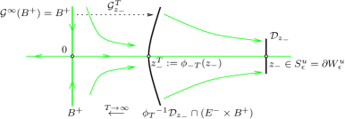
Figure 2: Backward $\lambda$-Lemma

Remark 1.3 (Contraction method proof of $\lambda$-Lemma).

The contraction method proof presented below has its own dis/advantages. On the worrying side, for $f\in C^{2}$, that is $X=-\nabla f\in C^{1}$, we only obtain $C^{0}$ convergence so far, whereas we do get $C^{1}$ convergence if $f$ is of class $C^{2,1}$ near $x$, e.g. if $f\in C^{3}$. On the bright side, we get rather useful quantitative control on each of the involved variables such as time $t$, the variable describing the dislocated disks, and their dependence on the base point; for details see Theorem 1.2. Most importantly, this quantitative control lends itself to construct foliations around critical points, foliations associated to global objects, namely sublevel sets, and to equip each leaf with its own semi-flow; see [Web14b, Web] for first applications.

Remark 1.4.

Theorem 1.2 is a family backward $\lambda$-Lemma, namely for the family of disks ${\mathcal{D}}=S^{u}_{\varepsilon}\times B^{+}_{\varkappa}$. Given a general hypersurface ${\mathcal{D}}^{\prime}$ whose intersection with the unstable manifold is transverse and equal to $S^{u}_{\varepsilon}$, one needs to change coordinates to bring ${\mathcal{D}}^{\prime}$ into the required normal form $S^{u}_{\varepsilon}\times B^{+}_{\varkappa}$. To achieve this apply the parametrized Implicit Function Theorem to construct a $C^{r}$ diffeomorphism of $V$ which is the identity outside a small neighborhood $U$ of the compact intersection locus $S^{u}_{\varepsilon}$ and maps the part of ${\mathcal{D}}^{\prime}$ near $S^{u}_{\varepsilon}$ to $S^{u}_{\varepsilon}\times B^{+}_{\varkappa}$ for some $\varkappa$.

We substituted the backward flow of the disk ${\mathcal{D}}_{z_{-}}$ by its pre-image ${\phi_{T}}^{-1}{\mathcal{D}}_{z_{-}}$, because there are interesting situations, cf. [Hen81], with only a forward semi-flow. For instance, the heat flow on the loop space of a closed Riemannian manifold [SW06] is just a forward semi-flow. Surprisingly, although there is no backward flow, there is a backward $\lambda$-Lemma[Web14a] under which the hypersurface ${\mathcal{D}}$ moves backward in time and foliates an open set. Furthermore, it is even still possible to construct a non-trivial Morse complex [Web13, Web14b]. Consequently the – in finite dimensions – common situation of a genuine forward and backward flow with stable and unstable manifolds, all being finite dimensional, allows for (too) many choices. In order to emphasize the necessary elements and, at the same time, to introduce the reader tacitly to the infinite dimensional heat flow scenario, we subject ourselves to the following convention.

Convention 1.5 (No backward Cauchy problem).

We shall use existence of a solution to the Cauchy problem only in forward time and ignore the backward Cauchy problem alltogether. However, on the unstable manifold there is still a natural procedure to define a backward flow; see Definition 3.3. Since there is no Cauchy problem involved, we will (and need to) use this so-called algebraic backward flow; this is coherent with the infinite dimensional case cited above. In finite dimensions the algebraic backward flow coincides with the one obtained via the Cauchy problem. So we do use a backward flow, but without solving the backward Cauchy problem and only along the unstable manifold.
To put things positively, our self-imposed lack of mathematical structure eliminates the possibility of choices and therefore reveals those elements which are essential to define a Morse complex – or even just an unstable manifold.

The simple but far reaching idea, see [Web14a, Web14b], which avoids any backward Cauchy problem is to look at the pre-image under the time-$T$-map of a given disk ${\mathcal{D}}_{q}(x)$ transverse at $q$ to the unstable manifold $W^{u}(x)$. The obvious but non-trivial problem is then to show that these sets are in fact submanifolds of $M$. To show this we shall write them locally near $x$ as graphs over the stable tangent space $E^{+}=T_{x}W^{s}(x)$ using the contraction method which in this case consists of interpreting the backward Cauchy problem as a “mixed Cauchy problem”. The latter can be reformulated in terms of the fixed point of a contraction, both depending on parameters. Thereby we obtain a new proof of the $\lambda$-Lemma in finite dimensions; see [Web14a] for the infinite dimensional semi-flow case of a parabolic PDE where this program has been carried out first. A key point of interest will be to control how the pre-images depend on time $T$.

Stable foliations

Borrowing from [Sal90] we define for each choice of constants ${\varepsilon},\tau>0$ a pair

$$\begin{split}N_{x}^{s}=N_{x}^{s}({\varepsilon},\tau):&=\left\{p\in M\mid\text{$f(p)\leq c+{\varepsilon}$, $f(\varphi_{\tau}p)\geq c-{\varepsilon}$}\right\}_{x},\end{split}$$ (3)

where $\{\ldots\}_{x}$ denotes the path connected component that contains $x$, and

$$L_{x}^{s}=L_{x}^{s}({\varepsilon},\tau):=\{p\in N_{x}^{s}\mid f(\varphi_{2\tau}p)\leq c-{\varepsilon}\}.$$ (4)

Figure 3 shows a typical

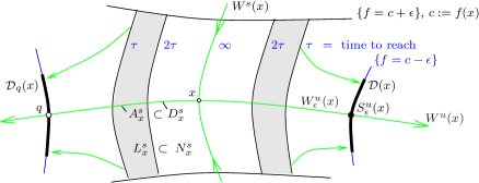
Figure 3: Conley pair $(N_{x}^{s},L_{x}^{s})$ associated to critical point $x$

such pair, illustrates what is called the exit set property of $L_{x}^{s}$, and indicates hypersurfaces which are characterized by the fact that each point reaches the level set $\{f=c-{\varepsilon}\}$ in the same time. The points on the stable manifold never reach level $c-{\varepsilon}$, so they are assigned the time label $\infty$. By the backward $\lambda$-Lemma, Theorem 1.2, these hypersurfaces foliate some neighborhood of $x$. However, the neighborhood and so the leaves have no global meaning so far. It is the content of Theorem 5.1 that the pairs $(N_{x}^{s},L_{x}^{s})$ which are defined in terms of level sets are foliations; for a first application see [Web].

Remark 1.6 (Forward $\lambda$-Lemma and unstable foliations).

Since the backward $\lambda$-Lemma as well as the stable foliations $(N_{x}^{s},L_{x}^{s})$ with respect to $f$ are of local nature at $x$ one can simply obtain the forward version of Theorem 1.2 and the unstable foliations $(N_{x}^{u},L_{x}^{u})$ with respect to $f$ by taking the former ones with respect to $-f$. (If necessary, cut off $-f$ to obtain a complete forward flow.)

2 Preliminaries

Throughout we denote by $\nabla=\nabla^{g}$ the Levi-Civita connection associated to the Riemannian metric $g$ on $M$ which we also denote by $\langle\cdot,\cdot\rangle$. Given a singularity $p$ of a vector field $X$ on $M$ we denote by $DX_{p}$ linearization $dX_{p}:T_{p}M\to T_{X(p)}TM\cong T_{p}M\oplus T_{p}M$ followed by projection onto the second component. The isomorphism is natural, because $X(p)=0$. There is the identity $DX_{p}=(\nabla\kern-2.15277pt{}_{\cdot}X)_{p}$.

Hessian and spectrum

By ${\rm Crit}f$ we denote the set of critical point of $f$. Given $p\in{\rm Crit}f$, in other words a singularity of $X=\nabla f$, then there is a linear symmetric operator $A=A_{p}:T_{p}M\to T_{p}M$ uniquely determined by the identity

$$\mathrm{Hess}_{p}f\,(v,w)=\langle Av,w\rangle$$ (5)

for all $v,w\in T_{p}M$. The bilinear form $\mathrm{Hess}_{p}f$ is defined in local coordinates in terms of the (symmetric) matrix with entries $({\partial}^{2}f/{\partial}x^{i}{\partial}x^{j})(p)$. It holds that $Av=D(\nabla f)_{p}v=(\nabla\kern-2.15277pt{}_{\tilde{v}}\nabla f)_{p}$ where $\tilde{v}$ is a vector field on $M$ with $\tilde{v}_{p}=v$. By symmetry the spectrum of the Hessian operator $A$ is real. If it does not contain zero, then $p$ is called a non-degenerate critical point of $f$.

Suppose $x$ is a non-degenerate critical point of $f$. Then by the spectral theorem for symmetric operators the spectrum of $A=A_{x}$ is given by $n$ reals

$$\lambda_{1}\leq\dots\leq\lambda_{k}<0<\lambda_{k+1}\leq\dots\leq\lambda_{n}$$ (6)

counting multiplicities. The distance $d>0$ between $0$ and the spectrum of $A$ is called the spectral gap of $A$. The number $k$ of negative eigenvalues is called the Morse index of the critical point $x$ and denoted by ${\rm ind}(x)$. Denote by $E^{-}$ and $E^{+}$ the span of all eigenvectors associated to negative and positive eigenvalues, respectively. Then there is the orthogonal splitting

$$T_{x}M=E^{-}\oplus E^{+}$$ (7)

with associated orthogonal projections $\pi_{-}:T_{x}M\to E^{-}$ and $\pi_{+}:T_{x}M\to E^{+}$. Since $A$ preserves $E^{-}$ and $E^{+}$ it restricts to linear operators $A^{-}:=A\circ\pi_{-}$ and $A^{+}:=A\circ\pi_{+}$ on $E^{-}$ and $E^{+}$, respectively. If $0<k<n$, then $\lambda_{1}<0<\lambda_{n}$.

Linearized equation and linearized flow

Linearizing the downward gradient equation (1) at a constant solution $u(t)\equiv p\in{\rm Crit}f$ in direction of a vector field $\xi:{\mathbb{R}}\to T_{p}M$ along $u$ leads to the linear autonomous ODE

$$\dot{\xi}(t)=-A\xi(t)$$ (8)

for $\xi$ where $A=A_{p}$ is the Hessian operator determined by (5).

Interpreting $-A:T_{p}M\to T_{p}M$ in (8) as a vector field on the manifold $T_{p}M$ it is easy to see that the flow generated by $-A$ is the 1-parameter family $\{\Phi_{t}\}_{t\in{\mathbb{R}}}$ of invertible linear operators on $T_{p}M$ given by

$$\Phi_{t}=e^{-tA}:=\sum_{j=0}^{\infty}\frac{(-t)^{j}}{j!}A^{j}.$$ (9)

If the spectrum of $A$ is given by $\{\lambda_{1},\dots,\lambda_{n}\}\subset{\mathbb{R}}$, then $\{e^{-t\lambda_{1}},\dots,e^{-t\lambda_{n}}\}\subset(0,\infty)$ is the spectrum of $e^{-tA}$. We will use $\Phi_{t}=e^{-tA}=e^{-tA^{-}}\oplus e^{-tA^{+}}$ only for $t\geq 0$. However, the part $e^{-tA^{-}}$ will be needed for all $t\in{\mathbb{R}}$. Since this part acts on the (linear) unstable manifold $E^{-}$ and is defined by a matrix exponential – thus without employing any backward Cauchy problem – there is no conflict with Convention 1.5.

Lemma 2.1 (Linearized flow satisfies linearized equation).

Given $p\in{\rm Crit}f$, then the family of linearizations $\{d\varphi_{t}(p)\}_{t\geq 0}$ coincides with the time-$t$-maps $\{\Phi_{t}\}_{t\geq 0}$ associated to the linearized vector field $-A=-D(\nabla f)_{p}$ on $T_{p}M$.

Proof.

See e.g. [Web06, Le. 2.5]. ∎

Proposition 2.2 (Exponential estimates).

Consider the Hessian operator $A=A^{-}\oplus A^{+}$ associated to a non-degenerate critical point $x$ of Morse index $k$ and with induced splitting $T_{x}M=E^{-}\oplus E^{+}$ provided by (7). Fix a constant $\mu$ in the spectral gap $[0,d]$ of $A$. In this case there are the estimates

$$\bigl{\|}e^{-tA^{+}}\bigr{\|}\leq e^{-t\lambda_{k+1}}\leq e^{-t\mu},\qquad\bigl{\|}e^{-tA^{-}}\bigr{\|}\leq e^{-t\lambda_{1}},$$

for every $t\geq 0$ and

$$\bigl{\|}e^{-tA^{+}}\bigr{\|}\leq e^{-t\lambda_{n}},\qquad\bigl{\|}e^{-tA^{-}}\bigr{\|}\leq e^{-t\lambda_{k}}\leq e^{t\mu},$$

for every $t\leq 0$. Thus $\mathopen{\|}e^{-tA}\mathclose{\|}\leq\max\{e^{-t\lambda_{k+1}},e^{-t\lambda_{1}}\}\leq\max\{e^{-t\mu},e^{-t\lambda_{1}}\}$ whenever $t\geq 0$ and $\mathopen{\|}e^{-tA}\mathclose{\|}\leq\max\{e^{-t\lambda_{n}},e^{-t\lambda_{k}}\}\leq\max\{e^{-t\lambda_{n}},e^{t\mu}\}$ whenever $t\leq 0$.

Proof.

Eigenvectors associated to $\lambda_{j}$ and $e^{-t\lambda_{j}}$ can be chosen equal. ∎

Exponential map

Given any point $q$ of our Riemannian manifold $M$, we denote by $\exp_{q}:T_{q}M\supset{\mathcal{O}}_{\iota_{q}}\to M$ the associated exponential map. Here ${\mathcal{O}}_{\iota_{q}}$ is the open ball whose radius $\iota_{q}>0$ is the injectivity radius of $\exp$ at the point $q$. The infimum $\iota\geq 0$ of $\iota_{q}$ over $M$ is called the injectivity radius of $M$. The map

$$\exp:TM\supset{\mathcal{O}}_{\iota}\to M$$

is called the exponential map of the Riemannian manifold. It is a piece of mathematical folklore that one can introduce global maps $E_{1}$ and $E_{2}$ which can be viewed as partial derivatives of the exponential map in the direction of $M$ and in the fiber direction, respectively. Also derivatives $E_{ij}$ of second and higher order can be introduced; see e.g. [Web14a, §2.1].

Theorem 2.3.

Given $u\in M$ and $\xi\in{\mathcal{O}}_{\iota_{u}}\subset T_{u}M$, then there are linear maps

$$E_{i}(u,\xi):T_{u}M\to T_{exp_{u}\xi}M,\qquad E_{ij}(u,\xi):T_{u}M\times T_{u}M\to T_{exp_{u}\xi}M,$$

for $i,j\in\{1,2\}$ such that the following is true. If $u:{\mathbb{R}}\to M$ is a smooth curve and $\xi,\eta$ are smooth vector fields along $u$ such that $\xi(s)\in{\mathcal{O}}_{\iota_{u(s)}}$ for every $s$, then the maps $E_{i}$ and $E_{ij}$ are characterized by the identities

$$\begin{split}\frac{d}{ds}\exp_{u}(\xi)&=E_{1}(u,\xi){\partial}_{s}u+E_{2}(u,\xi)\nabla\kern-2.15277pt{}_{s}\xi\\ \nabla\kern-2.15277pt{}_{s}\left(E_{1}(u,\xi)\eta\right)&=E_{11}(u,\xi)\left(\eta,{\partial}_{s}u\right)+E_{12}(u,\xi)\left(\eta,\nabla\kern-2.15277pt{}_{s}\xi\right)+E_{1}(u,\xi)\nabla\kern-2.15277pt{}_{s}\eta\\ \nabla\kern-2.15277pt{}_{s}\left(E_{2}(u,\xi)\eta\right)&=E_{21}(u,\xi)\left(\eta,{\partial}_{s}u\right)+E_{22}(u,\xi)\left(\eta,\nabla\kern-2.15277pt{}_{s}\xi\right)+E_{2}(u,\xi)\nabla\kern-2.15277pt{}_{s}\eta.\end{split}$$ (10)

These maps satisfy the identities

$$E_{1}(x,0)=E_{2}(x,0)={{\mathchoice{\rm 1\mskip-4.0mul}{\rm 1\mskip-4.0mul}{\rm 1\mskip-4.5mul}{\rm 1\mskip-5.0mul}}},\quad E_{11}(x,0)=E_{21}(x,0)=E_{22}(x,0)=0.$$ (11)

Tangent coordinates near critical point

Lemma 2.4.

Pick $p\in Critf$ and let $\iota_{p}>0$ be its injectivity radius. Then in the neighborhood $\exp_{p}{\mathcal{O}}_{\iota_{p}}$ of $p$ in $M$ the solutions to $\dot{u}=-(\nabla f)\circ u$ correspond via the identity $u(t)=\exp_{p}\xi(t)$ precisely to the solutions of the ODE

$$\dot{\xi}(t)+A\xi(t)=h(\xi(t)),\qquad h(\xi)=-E_{2}(p,\xi)^{-1}(\nabla f)_{\exp_{p}\xi}+A\xi,$$ (12)

where $\xi$ takes values in the open ball ${\mathcal{O}}_{\iota_{p}}\subset T_{p}M$ and $h(\xi)$ abbreviates $h(\xi(t))$.

Proof.

Given any smooth curve $\xi$ in ${\mathcal{O}}_{\iota_{p}}$, set $u(t)=\exp_{p}\xi(t)$. Take the derivative to get that $\dot{u}=E_{2}(p,\xi)\dot{\xi}$ pointwise in $t$. Thus we obtain that

$$E_{2}(p,\xi)\dot{\xi}=\dot{u}=-(\nabla f)\circ u=-E_{2}(p,\xi)A\xi-\left((\nabla f)_{\exp_{p}\xi}-E_{2}(p,\xi)A\xi\right)$$

pointwise in $t$ and where the last step is by adding zero. ∎

Lipschitz continuity of the non-linearity

Lemma 2.5 (Lipschitz near $p\in{\rm Crit}f$).

Recall that $f\in C^{r+1}(M,{\mathbb{R}})$ for $r\geq 1$. Fix $p\in{\rm Crit}f$ and let $\iota_{p}$ be its injectivity radius. Set $\rho_{0}:=\iota_{p}/4$. Then there is a continuous and non-decreasing function $\kappa:[0,\rho_{0}]\to[0,\infty)$ vanishing at $0$ such that the following is true. The non-linearity $h:B_{\rho_{0}}\to T_{p}M$ given by (12) is of class $C^{r}$. It satisfies $h(0)=0$ and $dh(0)=0$ and the Lipschitz estimate

$$\left\|h(\xi)-h(\eta)\right\|\leq\kappa(\rho)\left\|\xi-\eta\right\|$$

and its consequence

$$\left\|dh(\xi)v\right\|\leq\kappa(\rho)\left\|v\right\|$$ (13)

whenever $\mathopen{\|}\xi\mathclose{\|},\mathopen{\|}\eta\mathclose{\|}\leq\rho\leq\rho_{0}$ and $v\in T_{p}M$. If $f$ is of class $C^{2,1}$ locally near $p$, then there is a constant $\kappa_{*}>0$ such that $dh$ satisfies the Lipschitz estimate

$$\begin{split}\left\|dh(\xi)v-dh(\eta)v\right\|&\leq\kappa_{*}\left\|\xi-\eta\right\|\left\|v\right\|,\end{split}$$

whenever $\mathopen{\|}\xi\mathclose{\|},\mathopen{\|}\eta\mathclose{\|}\leq\rho\leq\rho_{0}$ and $v\in T_{p}M$.

Proof of the Lipschitz Lemma 2.5.

That $f\in C^{r+1}$ implies $h\in C^{r}$ follows immediately from the definition of $h$; see (12). Pick $\xi,\eta\in B_{\rho_{0}}$ and set $X:=\eta-\xi$. It is useful to view $\xi$ as being fixed and $\eta(X)=\xi+X$ as depending on $X$. Consider the map defined by

$$\begin{split}I(X):=h(\xi)-h(\eta)&=-E_{2}(p,\xi)^{-1}(\nabla f)_{\exp_{p}\xi}+A\xi\\ &\quad+E_{2}(p,\xi+X)^{-1}(\nabla f)_{\exp_{p}(\xi+X)}-A(\xi+X)\end{split}$$

and note that $I(0)=0$. Moreover, for any $v\in T_{p}M$ it holds that

$$\begin{split}dI(X)v&=\left.\tfrac{D}{d\tau}\right|_{0}I(X+\tau v)\\ &=-E_{2}(p,\xi+X)^{-1}E_{22}(p,\xi+X)\left[(\nabla f)_{\exp_{p}(\xi+X)},E_{2}(p,\xi+X)^{-1}v\right]\\ &\quad+E_{2}(p,\xi+X)^{-1}D(\nabla f)_{\exp_{p}(\xi+X)}E_{2}(p,\xi+X)v-Av\end{split}$$

where brackets $[\dots]$ indicate (multi)linearity. Thus we obtain that

$$\begin{split}\mathopen{\|}h(\xi)-h(\eta)\mathclose{\|}&=\mathopen{\|}I(X)\mathclose{\|}=\mathopen{\|}I(X)-I(0)\mathclose{\|}=\mathopen{\|}dI(\sigma X)X\mathclose{\|}\\ &\leq\mathopen{\|}{E_{2}}^{-1}\mathclose{\|}_{L^{\infty}(B_{3\rho_{0}})}^{2}\mathopen{\|}E_{22}\mathclose{\|}_{L^{\infty}(B_{3\rho})}\mathopen{\|}(\nabla f)_{\exp_{p}}\mathclose{\|}_{L^{\infty}(B_{3\rho})}\mathopen{\|}X\mathclose{\|}\\ &\quad+\mathopen{\|}{E_{2}}^{-1}D(\nabla f)_{\exp_{p}}E_{2}-A\mathclose{\|}_{L^{\infty}(B_{3\rho})}\mathopen{\|}X\mathclose{\|}\\ &=:\kappa(\rho)\mathopen{\|}\xi-\eta\mathclose{\|}\end{split}$$

where for instance $E_{2}$ abbreviates $E_{2}(p,\cdot)$ and $L^{\infty}$ denotes the sup-norm. Moreover, existence of some constant $\sigma\in[0,1]$ is asserted by Taylor’s theorem. That the function $\kappa(\rho)$ is non-decreasing is due to the fact that the supremum is taken over the closed ball of radius $3\rho$. Indeed the supremum is obviously non-decreasing if it is taken over larger balls, that is if $\rho$ grows. For $\rho=0$ all maps are evaluated at the origin of $T_{p}M$, thus $\kappa(0)=0$ since $E_{22}(p,0)=0$ and $E_{2}(p,0)={{\mathchoice{\rm 1\mskip-4.0mul}{\rm 1\mskip-4.0mul}{\rm 1\mskip-4.5mul}{\rm 1\mskip-5.0mul}}}$ by (11) and since $D(\nabla f)_{p}-A=0$. This proves the Lipschitz estimate. Concerning its consequence recall that $dh(\xi)v=\lim_{\tau\to 0}\frac{h(\xi+\tau v)-h(\xi)}{\tau}$ and apply the Lipschitz estimate.

Concerning the Lipschitz estimate for $dh$ note that by (12) we get that

$$\begin{split}dh(\xi)v=\left.\tfrac{D}{d\tau}\right|_{0}h(\xi+\tau v)&=E_{2}(p,\xi)^{-1}E_{22}(p,\xi)\left[(\nabla f)_{\exp_{p}(\xi)},E_{2}(p,\xi)^{-1}v\right]\\ &\quad-E_{2}(p,\xi)^{-1}D(\nabla f)_{\exp_{p}(\xi)}E_{2}(p,\xi)v+Av.\end{split}$$

Since by assumption $D(\nabla f)_{\exp_{p}(\cdot)}$ is locally Lipschitz near the origin, so is $dh$. ∎

Cauchy problem and integral equation

Proposition 2.6.

Given a non-degenerate critical point $x\in{\rm Crit}f$, let $\iota_{x}$ be its injectivity radius and consider the ODE (12) in $T_{x}M$ with non-linearity $h$. Fix a radius

$$\rho_{0}\in\left(0,\min\{1,\iota_{x}/4\}\right]$$ (14)

sufficiently small such that the image $\exp_{x}B_{\rho_{0}}\subset M$ of the closed ball $B_{\rho_{0}}\subset T_{x}M$ contains no critical point of $f$ other than $x$. Pick $T\geq 0$ and assume that $\xi:[0,T]\to T_{x}M$ is a map bounded by $\rho_{0}$. Then the following are equivalent.

1. The map $\xi:[0,T]\to T_{x}M$ of class $C^{1}$ is the (unique) solution of the Cauchy problem given by the localized downward gradient flow equation (12) with initial value $\xi(0)$.

2. The map $\xi:[0,T]\to T_{x}M$ is continuous and satisfies the integral equation or representation formula

   $$\begin{split}\xi(t)&=e^{-tA}\pi_{+}\xi(0)+\int_{0}^{t}e^{-(t-\sigma)A}\pi_{+}h(\xi(\sigma))\,d\sigma\\ &\quad+e^{-(t-T)A^{-}}\pi_{-}\xi(T)-\int_{t}^{T}e^{-(t-\sigma)A^{-}}\pi_{-}h(\xi(\sigma))\,d\sigma\end{split}$$ (15)

   for every $t\in[0,T]$. In the limit $T\to\infty$ term three in the sum disappears.

Proof.

Essentially variation of constants; cf. [Tes12, §9.2] or [Jos11, §7.3]. ∎

3 Invariant manifolds

Suppose $x\in M$ is a hyperbolic singularity of the vector field $X=-\nabla f$, that is a non-degenerate critical point of $f$. The stable manifold of the flow-invariant set $\{x\}$ is defined by

$$W^{s}(x):=\bigl{\{}q\in M\,\big{|}\,\text{$\lim_{t\to\infty}\varphi_{t}q$ exists and is equal to $x$}\bigr{\}}.$$ (16)

In case of a genuine complete flow one simply considers the limit $t\to-\infty$ to define the unstable manifold $W^{u}(x)$. Note that – despite the naming – these sets are, at this stage, nothing but sets. They are invariant under the flow though. A common strategy to endow them with a differentiable structure is to represent them locally near $x$ as graphs of differentiable maps and then use the flow and flow invariance to transport the resulting coordinate charts to any location on the un/stable manifold. To carry out the graph construction one introduces in an intermediate step what is called local un/stable manifolds.

Unstable manifold theorem

In view of our Convention 1.5 to ignore the backward Cauchy problem, already defining $W^{u}(x)$ by the analogue of (16) is not possible. A way out is to consider an asymptotic boundary value problem instead: Consider the set of all forward semi-flow lines that emanate at time $-\infty$ from the non-degenerate critical point $x$, then evaluate each such solution at time zero and define $W^{u}(x)$ to be the set of all these evaluations. In symbols, the unstable manifold of $x$ is defined by

$$W^{u}(x):=\bigl{\{}u(0)\,\big{|}\,\text{$u:(-\infty,0]\to M$, (\ref{eq:DGE}), $\lim_{t\to-\infty}u(t)=x$}\bigr{\}}.$$ (17)

It is non-empty since the constant trajectory $u\equiv x$ contributes the element $x$.

Theorem 3.1 (Unstable manifold theorem).

Non-degeneracy of $x$ together with $\varphi$ being a gradient flow implies that the unstable manifold $W^{u}(x)$ is an embedded submanifold of $M$ of class $C^{r}$ tangent at $x$ to the vector subspace $E^{-}\subset T_{x}M$ of dimension $k={\rm ind}(x)$ and diffeomorphic to $E^{-}$.

Corollary 3.2 (Descending disks).

Given $x\in{\rm Crit}f$ non-degenerate, then there is a constant ${\varepsilon}_{x}>0$ such that the following is true.

1. Each descending disk defined by

   $$W^{u}_{\varepsilon}(x):=W^{u}(x)\cap\{f\geq f(x)-{\varepsilon}\},\qquad{\varepsilon}\in(0,{\varepsilon}_{x}],$$ (18)

   is $C^{r}$ diffeomorphic, as a manifold-with-boundary, to the closed unit disk ${\mathbb{D}}^{k}\subset{\mathbb{R}}^{k}$ where $k={\rm ind}(x)$. The boundary

   $$S^{u}_{\varepsilon}(x)=W^{u}(x)\cap\{f=f(x)-{\varepsilon}\}$$

   of a descending disk is called a descending sphere.

2. Each open neighborhood of $x$ in $M$, thus each open neighborhood of $x$ in $W^{u}(x)$, contains a descending disk.

Suggestion for proof..

Apply Theorem 3.1 and the version of the Transversality Theorem for manifolds-with-boundary, see [Hir76, Ch. 1 §4], to obtain the $C^{r}$ manifold structure of the descending disk. Use the Morse Lemma [Hir76], which causes loss of regularity, only to control the locus. ∎

The proof of the unstable manifold Theorem 3.1 is a Corollary of the local unstable manifold Theorem 3.4 below. The standard argument is to use the forward flow to move the coordinate charts provided by Theorem 3.4 near $x$ to any point of $W^{u}(x)$. This shows that $W^{u}(x)$ is injectively immersed. Now exploit the gradient flow property. To prove Theorem 3.4 we need a backward flow, but only on the unstable manifold, which is coherent with Convention 1.5.

Definition 3.3 (Algebraic backward flow on unstable manifold).

Given $u(0)\in W^{u}(x)$, set $q:=u(0)$ and define $\psi_{-t}q:=u(-t)$ for $t\geq 0$. Note that $\psi_{-t}\psi_{-s}=\psi_{-t-s}$ and that $\psi_{-t}q$ solves the backward time Cauchy problem (1) with initial value $q$. Therefore it doesn’t violate Convention 1.5 if, for any $q\in W^{u}(x)$, we use the notation $\varphi_{t}q$ for any time $t$, positive or negative.

While $W^{u}(x)$ is obviously backward and forward flow invariant, a descending disk still is backward invariant since its boundary lies in a level set.

Local unstable manifold theorem

We wish to prove that $W^{u}(x)$ carries locally near $x$ the structure of a manifold.

Figure 4: Spectral gap $d$

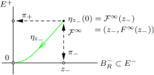
Figure 5: Graph map ${\mathcal{F}}^{\infty}:B^{-}_{R}\to T_{x}M$

Theorem 3.4 (Local unstable manifold, Hadamard-Perron [Had01, Per28]).

Assuming (H1–H2) in Definition 1.1 there is a constant $\rho=\rho(\lambda)\in(0,\frac{\rho_{0}}{2})$ such that the following is true. A neighborhood of $0$ in the local unstable manifold

$$W^{u}(0,B_{\rho_{0}}):=\Bigl{\{}\eta(0)\,\big{|}\,\text{ $\eta:(-\infty,0]\to B_{\rho_{0}}$, (\ref{eq:f}), $\lim_{t\to-\infty}\eta(t)=0$}\Bigr{\}}$$ (19)

is a graph over the radius $R=\frac{\rho}{2}$ ball $B^{-}_{R}\subset E^{-}$ and this graph is tangent to $E^{-}$ at $0$. More precisely, there is a $C^{r}$ map

$${\mathcal{F}}^{\infty}=\left(id,F^{\infty}\right):B^{-}_{R}\to E^{-}\oplus E^{+},\quad F^{\infty}(0)=0,\quad dF^{\infty}(0)=0,$$ (20)

whose image is a neighborhood of $0$ in $W^{u}(0,B_{\rho_{0}})$. Moreover, it holds that $\left\|\phi_{t}\eta_{0}\right\|\leq\rho e^{t\lambda}$ for every $t\leq 0$ and uniformly in $\eta_{0}\in{\mathcal{F}}^{\infty}(B^{-}_{R})$; see Figure 5.

We sketch the proof of the theorem by the contraction method. Pick an element $z_{-}\in E^{-}$ near the origin. Our object of interest is a backward flow line $\eta:(-\infty,0]\to B_{\rho_{0}}$ whose value at time zero projects to $z_{-}$ under $\pi_{-}$ and which emanates from the origin asymptotically at time $t=-\infty$. For any sufficiently small constant $\rho\in(0,\frac{\rho_{0}}{2})$ the complete metric space

$$\begin{split}Z^{-}=Z^{-}_{\lambda,\rho}:=\Bigl{\{}\eta\in C^{0}((-\infty,0],T_{x}M)\,\,\Big{|}\,\,\left\|\eta\right\|_{\exp}^{-}:=\sup_{t\leq 0}e^{-t\lambda}\left\|\eta(t)\right\|\leq\rho\Bigr{\}}\end{split}$$

carries the contraction given by

$$\begin{split}\left(\Phi_{z_{-}}\eta\right)(s):=e^{-sA^{-}}z_{-}&-\int_{s}^{0}e^{-(s-\sigma)A^{-}}\pi_{-}h(\eta(\sigma))d\sigma\\ &+\int_{-\infty}^{s}e^{-(s-\sigma)A}\pi_{+}h(\eta(\sigma))d\sigma.\end{split}$$ (21)

Its (unique) fixed point $\eta_{z_{-}}$ is the desired flow line. Define the graph map by $F^{\infty}(z_{-}):=\pi_{+}(\eta_{z_{-}}(0))$ as illustrated by Figure 5 and denote by $B^{-}_{R}\subset E^{-}$ the ball of radius $R=\frac{\rho}{2}<\frac{\rho_{0}}{4}$ about $0$.

Stable manifold theorem

Whereas the stable manifold is easier to define – given only a forward flow – than the unstable manifold, the step from local to global is not obvious any more, given Convention 1.5. We shall use this oportunity to promote Henry’s [Hen81], widely unkown as it seems, argument to pull back the local coordinate charts near $x$ in the backward time direction utilizing only the forward flow.

Theorem 3.5 (Stable manifold theorem).

Non-degeneracy of $x$ together with $\varphi$ being a gradient flow implies that the stable manifold $W^{s}(x)$ defined by (16) is an embedded submanifold of $M^{n}$ of class $C^{r}$ tangent at $x$ to the vector subspace $E^{+}\subset T_{x}M$. Thus $\dim W^{s}(x)$ is equal to the Morse co-index $n-k$ of $x$.

Remark 3.6.

The ascending disk $W^{s}_{\varepsilon}(x)$ and the ascending sphere $S^{s}_{\varepsilon}(x)$ are defined as in Corollary 3.2, just replace the superlevel set $\{f\geq f(x)-{\varepsilon}\}$ by the sublevel set $\{f\leq f(x)+{\varepsilon}\}$. They also have analogous properties, in the assertions just replace $k$ by $n-k$ where $n=\dim M$.

Theorem 3.7 (Local stable manifold, Hadamard-Perron [Had01, Per28]).

Assuming (H1–H2) in Definition 1.1 there is a constant $\rho=\rho(\lambda)\in(0,\frac{\rho_{0}}{2})$ such that a neighborhood of $0$ in the local stable manifold

$$W^{s}(0,B_{\rho_{0}}):=\Bigl{\{}z\in B_{\rho_{0}}\,\big{|}\,\text{$\phi_{t}z\in B_{\rho_{0}}$ $\forall t>0$ and $\lim_{t\to\infty}\phi_{t}z=0$}\Bigr{\}}$$ (22)

is a graph over the radius $R=\frac{\rho}{2}$ ball $B^{+}_{R}\subset E^{+}$ and this graph is tangent to $E^{+}$ at $0$. More precisely, there is a $C^{r}$ map

$${\mathcal{G}}^{\infty}=\left(G^{\infty},id\right):B^{+}_{R}\to E^{-}\oplus E^{+},\quad G^{\infty}(0)=0,\quad dG^{\infty}(0)=0,$$ (23)

whose image is a neighborhood of $0$ in $W^{s}(0,B_{\rho_{0}})$. Moreover, it holds that $\left\|\phi_{t}\xi_{0}\right\|\leq\rho e^{-t\lambda}$ for every forward time $t\geq 0$ and uniformly in $\xi_{0}\in{\mathcal{G}}^{\infty}(B^{+}_{R})$.

The proof of Theorem 3.7 is by the contraction method. In fact, our proof of the Backward $\lambda$-Lemma, Theorem 1.2, presented below generalizes the contraction method proof from invariant manifolds, which is well known, to invariant foliations. The details missing in the following sketch of proof can be easily recovered by formally setting $T=\infty$ in the proof of Theorem 1.2.
Pick $z_{+}\in E^{+}$ near $0$. Our object of interest is a flow line $\xi:[0,\infty)\to B_{\rho_{0}}$ whose initial value projects to $z_{+}$ under $\pi_{+}$ and which converges to $0$, as $t\to\infty$. For any sufficiently small constant $\rho\in(0,\frac{\rho_{0}}{2})$ the complete metric space

$$\begin{split}Z=Z_{\lambda,\rho}:=\Bigl{\{}\xi\in C^{0}([0,\infty),T_{x}M)\,\,\big{|}\,\,\left\|\xi\right\|_{\exp}:=\sup_{t\geq 0}e^{t\lambda}\left\|\xi(t)\right\|\leq\rho\Bigr{\}},\end{split}$$ (24)

carries a contraction defined by

$$(\Psi_{z_{+}}\xi)(t)=e^{-tA}z_{+}+\int_{0}^{t}e^{-(t-\sigma)A}\pi_{+}h(\xi(\sigma))d\sigma-\int_{t}^{\infty}e^{-(t-\sigma)A^{-}}\pi_{-}h(\xi(\sigma))d\sigma.$$

Moreover, by the representation formula (15) for $T=\infty$ the (unique) fixed point $\xi_{z_{+}}$ is our object of interest. For $R=\frac{\rho}{2}<\frac{\rho_{0}}{4}$ the map

$$\begin{split}G^{\infty}:B^{+}_{R}&\to E^{-},\qquad\qquad\quad B^{+}_{R}:=\left\{z_{+}\in E^{+}:\left\|z_{+}\right\|\leq\rho/2\right\},\\ z_{+}&\mapsto\pi_{-}\left(\xi_{z_{+}}(0)\right)\end{split}$$

has the properties asserted by Theorem 3.7; see also [CH82, Sec. 3.6].

Remark 3.8.

Further methods to prove the local (un)stable manifold theorems:

• Graph transform method: A geometrically appealing method, nicely sketched in [PdM82, p.80]; for details see [Shu87].

• Irwin’s space of sequences: See former two references. Another excellent reference for those who care about details is Zehnder’s recent book [Zeh10].

Proof of the stable manifold Theorem 3.5 (Henry [Hen81, Thm. 6.1.9]).

By Theorem 3.7 the stable manifold is locally near $x$ a $C^{r}$ submanifold of $M$ of dimension $n-k$ where $k$ is the Morse index of $x$ and $n=\dim M$. Thus there is a neighborhood $\Sigma$ of $x$ in $W^{s}(x)$ which is represented as a zero set $\{y\in U\mid h(y)=0\}$ where $U$ is an open set in $M$ and $h:U\to{\mathbb{R}}^{k}$ is a $C^{r}$ map such that $dh_{y}:T_{y}M\to{\mathbb{R}}^{k}$ is surjective at each point

$$y\in h^{-1}(0)=U\cap\Sigma=U\cap W^{s}(x).$$

Note that here only the first identity is part of the submanifold property of $\Sigma$. To obtain the second identity choose $U$ smaller, if necessary, and use the fact that a flow line of a gradient flow cannot come back to itself asymptotically.

Nearby arbitrary elements $q_{0}$ of $W^{s}(x)$ one obtains local submanifold charts as follows. Pick $T\geq 0$ such that $\varphi_{T}q_{0}\in\Sigma$ and consider the $C^{r}$ map

$$h\circ\varphi_{T}:U_{T}\stackrel{{\scriptstyle\varphi_{T}}}{{\longrightarrow}}U\stackrel{{\scriptstyle h}}{{\longrightarrow}}{\mathbb{R}}^{k},\qquad U_{T}:={\varphi_{T}}^{-1}(U),$$

whose zero set is $U_{T}\cap W^{s}(x)$; see Figure 6. The pre-image $U_{T}$ is an open neighborhood of $q_{0}$ in $M$ since $U$ is open and $\varphi_{T}$ is continuous. By the regular value theorem it remains to show that the map

$$d(h\circ\varphi_{T})_{q}:T_{q}M\stackrel{{\scriptstyle d(\varphi_{T})_{q}}}{{\longrightarrow}}T_{y=\varphi_{T}q}M\stackrel{{\scriptstyle dh_{y}}}{{\longrightarrow}}{\mathbb{R}}^{k}$$

is surjective whenever $q\in(h\circ\varphi_{T})^{-1}(0)=U_{T}\cap W^{s}(x)$. Since $dh_{\varphi_{T}q}$ is surjective it suffices to show that $d(\varphi_{T})_{q}$ is surjective. The following argument avoids backward flows. In finite dimensions surjectivity of $d(\varphi_{T})_{q}$ is equivalent to dense range which itself is equivalent, even in the general Banach space case, to injectivity of the adjoint (or transposed) operator $(d\varphi_{T}|_{q})^{*}$. But the latter is equivalent to backward uniqueness of the (forward Cauchy problem associated to the) adjoint equation. In our case $A=A^{*}$ so the adjoint equation is just the linearized equation itself. But an ODE associated to a Lipschitz continuous vector field exhibits forward and backward uniqueness; see e.g. [AL93]. ∎

Figure 6: Henry’s proof: pull back coordinate charts by forward time-$T$-map

Convenient coordinates

Suppose the local setup of (H1–H2) in Definition 1.1. Namely fix a constant $\lambda$ in the spectral gap $(0,d)$ and recall that the local flow $\phi_{t}$ acting on the ball $B_{\rho_{0}}$ in $T_{x}M=X=E^{-}\oplus E^{+}$ is generated by the ODE $\dot{\zeta}+A\zeta=h(\zeta)$ where the non-linearity $h$ is given by (12). Consider the balls $B^{-}_{R}\subset E^{-}$ and $B^{+}_{R}\subset E^{+}$ of radius $R(x,\rho_{0},\lambda)=\frac{\rho}{2}<\frac{\rho_{0}}{4}$ with $B^{-}_{R}\times B^{+}_{R}\subset B_{\rho_{0}/2}$ and the $C^{r}$ graph maps $F^{\infty}:B^{-}_{R}\to E^{+}$ and $G^{\infty}:B^{+}_{R}\to E^{-}$ provided by the local (un)stable manifold Theorems 3.4 and 3.7. Use the fact that the graph ${\mathcal{F}}^{\infty}(B^{-}_{R})$ is tangent to $E^{-}$ at $0$, similarly for ${\mathcal{G}}^{\infty}(B^{+}_{R})$, to see that choosing the radius $R>0$ smaller, if necessary, one can arrange that both graphs simultaneously satisfy inclusions

$${\mathcal{F}}^{\infty}(B^{-}_{R})\subset\left(B^{-}_{R}\times B^{+}_{R}\right),\qquad{\mathcal{G}}^{\infty}(B^{+}_{R})\subset\left(B^{-}_{R}\times B^{+}_{R}\right).$$

On the other hand, by Corollary 3.2 and Remark 3.6 there is a (small) constant $2\varsigma>0$ such that there are inclusions of descending and ascending disks

$$W^{u}_{2\varsigma}\subset{\mathcal{F}}^{\infty}(B^{-}_{R}),\qquad W^{s}_{2\varsigma}\subset{\mathcal{G}}^{\infty}(B^{+}_{R}).$$ (25)

Set

$$D^{-}:=\pi_{-}W^{u}_{2\varsigma},\qquad D^{+}:=\pi_{+}W^{s}_{2\varsigma},\qquad V:=D^{-}\times D^{+}.$$ (26)

Then by the graph property of ${\mathcal{F}}^{\infty}$ and ${\mathcal{G}}^{\infty}$ it holds that ${\mathcal{F}}^{\infty}(D^{-})=W^{u}_{2\varsigma}$ and ${\mathcal{G}}^{\infty}(D^{+})=W^{s}_{2\varsigma}$ as illustrated by the left part of Figure 7. Consequently $D^{\pm}$ is a disk, that is a set diffeomorphic to a closed ball. Note that

$$W^{u}_{2\varsigma} =W^{u}(0,V)=V\cap W^{u}(0,B_{\rho_{0}}),$$ (27)

$$W^{s}_{2\varsigma} =W^{s}(0,V)\hskip 0.56917pt=V\cap W^{s}(0,B_{\rho_{0}}),$$

by negative and positive invariance under $\phi$ of $W^{u}_{2\varsigma}$ and $W^{s}_{2\varsigma}$, respectively. Following Palis and de Melo [PdM82, Ch. 2 §7] observe that the $C^{r}$ map

$$\vartheta(x,y):=\left(x-G^{\infty}(y),y-F^{\infty}(x)\right)$$

defined on $B^{-}_{R}\times B^{+}_{R}$ satisfies $\vartheta(0)=0$ and $d\vartheta(0)={{\mathchoice{\rm 1\mskip-4.0mul}{\rm 1\mskip-4.0mul}{\rm 1\mskip-4.5mul}{\rm 1\mskip-5.0mul}}}$. In particular, it is a diffeomorphism locally near the fixed point $0$. Choosing $R$ and $2\varsigma$ smaller, if necessary, we assume without loss of generality that $\vartheta$ is a diffeomorphism onto its image. Note that $\vartheta(x,0)=(x,-F^{\infty}(x))$ and $\vartheta(0,y)=(-G^{\infty}(y),y)$. Consequently the map $\vartheta$ diffeomorphically maps ${\mathcal{F}}^{\infty}(D^{-})=W^{u}_{2\varsigma}$ to the disk $D^{-}$ and similarly for $W^{s}_{2\varsigma}$ and $D^{+}$; see Figure 7.

Figure 7: Local (un)stable manifolds get flattened out

Our new local model will be the product of disks $V:=D^{-}\times D^{+}$ acted upon by the new local flow $\vartheta_{*}\phi_{t}=\phi_{t}\circ\vartheta\circ{\phi_{t}}^{-1}$ (denoted again by $\phi_{t}$ in Remark 3.9) whose local unstable and stable manifolds are $D^{-}$ and $D^{+}$, respectively. Note that the latter represent the descending disk $W^{u}_{2\varsigma}(x)$ and the ascending disk $W^{s}_{2\varsigma}(x)$ in this new local model. The ODE which generates the flow $\vartheta_{*}\phi_{t}$ arises by re-doing Lemma 2.4 starting from the “Ansatz” $u(t)=\exp_{x}\left({\vartheta}^{-1}\xi(t)\right)$ for $\xi$. Obviously the new ODE is similar to (12) involving, in addition, the diffeomorphism $\vartheta$ and its linearization. Since $\vartheta$ is of class $C^{r}$ and defined on the compact set $V$ it admits uniform $C^{r}$-bounds. Therefore relevant estimates for the new and the old ODE are equivalent up to constants. This justifies to simplify notation as follows.

Remark 3.9 (Coordinates with flattened local manifolds).

By the discussion above and in order to simplify notation we will, without loss of generality, continue to work with the ODE (12), that is we omit $\vartheta$ in our formulas, and assume that the local (un)stable manifolds $W^{u}_{2\varsigma}$ and $W^{s}_{2\varsigma}$ for the (new) local flow $\phi$ on $V$ are disks $D^{-}\subset E^{-}$ and $D^{+}\subset E^{+}$. To summarize we assume that

$$V:=D^{-}\times D^{+}\subset B^{-}_{R}\times B^{+}_{R}\subset B_{1},\quad D^{-}=W^{u}_{2\varsigma},\quad D^{+}=W^{s}_{2\varsigma},$$ (28)

as illustrated by Figure 1 and where $\varsigma>0$ has been fixed according to (25).

4 Proof of backward $\lambda$-Lemma

Suppose ${\rm ind}(x)=k\in\{1,\dots,n-1\}$, so the smallest and largest eigenvalue of the Hessian operator $A=A_{x}$ satisfy $\lambda_{1}<0<\lambda_{n}$. Consider the continuous function $\kappa(\rho)$ with $\kappa(0)=0$ and the Lipschitz constant $\kappa_{*}>0$ of the non-linearity $h$ provided by Lemma 2.5. Pick an exponential decay rate $\lambda\in(0,d)$ for the elements of the complete metric space $Z^{T}$ to be defined below and consider the two constants $\delta\in\left(0,\min\{1,\tfrac{d-\lambda}{2}\}\right)$ and $\mu\in\left(\lambda,\tfrac{d+\lambda}{2}\right)\subset(\lambda,d)$ defined in Figure 5. To ensure the second of the two endpoint conditions in (32) set

$$T_{1}=T_{1}(\lambda,\varkappa):=-\frac{\ln\varkappa}{\lambda}\geq 0.$$ (29)

Fix $\rho=\rho(\lambda)\in(0,1)$ sufficiently small such that

$$\kappa(\rho)\left(\frac{4}{\lambda}+\frac{1}{\delta}+1\right)\leq\frac{1}{8}$$ (30)

and such that the closed $\rho$-neighborhood $U_{\rho}(W^{u}_{\varsigma})$ in $X$ of the descending disk is contained in $V=D^{-}\times D^{+}\subset B_{1}$; see (28). Observe that in this case the radius $\frac{\rho}{2}$ ball $B^{+}\subset E^{+}$ is contained in $D^{+}$. Fix $T_{2}=T_{2}(\mu)>0$ such that $e^{-T_{2}\mu/4}\leq 1/8$; this will be used in Step 5. Set

$$T_{0}=T_{0}(\lambda,\mu(\lambda),\varkappa):=\max\{T_{1},T_{2},1\}\geq 1.$$ (31)

Remark 4.1 (Mixed Cauchy problem).

The key observation to represent the pre-image ${\phi_{T}}^{-1}{\mathcal{D}}_{z_{-}}$ under the time-$T$-map $\phi_{T}$ as a graph over the stable tangent space $E^{+}$ is the fact that there is a well posed mixed Cauchy problem. Namely, instead of prescribing precisely the endpoint, by the representation formula (15) it makes sense to prescribe only the ($\pi_{+}$)-part of the initial point, but in addition the ($\pi_{-}$)-part of the endpoint. This way one circumvents using a general backward flow – only the (by Convention 1.5 legal) algebraic one on the unstable manifold is used; cf. [Web14a, Rmk. 3].

We prove below that for each $z_{+}\in E^{+}$ with $\mathopen{\|}z_{+}\mathclose{\|}\leq\rho/2$ there is precisely one flow line $\xi=\xi_{z_{-},z_{+}}^{T}$ with initial condition $\pi_{+}\xi(0)=z_{+}$ and endpoint condition $\xi(T)\in{\mathcal{D}}_{z_{-}}$. The latter is equivalent to

$$\pi_{-}\xi(T)={z_{-}}\quad\wedge\quad\left\|\xi(T)-{z_{-}}\right\|\leq\varkappa.$$ (32)

The key step to determine the unique semi-flow line $\xi$ associated to the triple $(T,{z_{-}},z_{+})$ is to set up a strict contraction $\Psi^{T}$ on a complete metric space $Z^{T}$ whose (unique) fixed point is $\xi$. More precisely, define

$$Z^{T}=Z^{T,{z_{-}}}_{\lambda,\rho}:=\left\{\xi\in C^{0}([0,T],X)\,\colon\left\|\xi-\phi_{\cdot}{z_{-}^{T}}\right\|_{\exp}\leq\rho\right\},$$ (33)

where ${z_{-}^{T}}:=\phi_{-T}({z_{-}})$ and

$$\left\|\xi\right\|_{\exp}=\left\|\xi\right\|_{\exp,T}:=\max_{t\in[0,T]}e^{t\lambda}\left\|\xi(t)\right\|,$$ (34)

and consider the operator $\Psi^{T}=\Psi^{T}_{{z_{-}},z_{+}}$ defined for $\xi\in Z^{T}$ by

$$\begin{split}\left(\Psi_{{z_{-}},z_{+}}^{T}\xi\right)(t)&:=e^{-tA}z_{+}+\int_{0}^{t}e^{-(t-\sigma)A}\pi_{+}h(\xi(\sigma))\,d\sigma\\ &\quad+e^{-(t-T)A^{-}}{z_{-}}-\int_{t}^{T}e^{-(t-\sigma)A^{-}}\pi_{-}h(\xi(\sigma))\,d\sigma\end{split}$$ (35)

for every $t\in[0,T]$. The fixed points of $\Psi^{T}$ correspond to the desired flow trajectories by Proposition 2.6. In Step 1 and Step 2 below we show that $\Psi^{T}$ is a strict contraction on $Z^{T}$. Hence by the Banach-Cacciopoli Fixed Point Theorem, see e.g. [CH82, §2.2], it admits the unique fixed point $\xi_{{z_{-}},z_{+}}^{T}$ and we define the map

$$G^{T}:S^{u}_{\varepsilon}\times B^{+}\to E^{-},\qquad\left({z_{-}},z_{+}\right)\mapsto\pi_{-}\xi_{{z_{-}},z_{+}}^{T}(0)=:G^{T}_{z_{-}}(z_{+}).$$ (36)

For latter use we calculate for $t\in[0,T]$ and $\alpha>0$ the integrals

$$\int_{0}^{t}e^{-(t-\sigma)\alpha}\,d\sigma=\frac{1-e^{-t\alpha}}{\alpha},\qquad\int_{t}^{T}e^{(t-\sigma)\alpha}\,d\sigma=\frac{1-e^{(t-T)\alpha}}{\alpha}.$$ (37)

The proof takes six steps. Fix ${z_{-}}\in S^{u}_{\varepsilon}$ and $z_{+}\in B^{+}$. Abbreviate $\Psi^{T}=\Psi_{{z_{-}},z_{+}}^{T}$.

Step 1. For $T>0$ the set $Z^{T}$ equipped with the exp norm metric is a complete metric space, any $\xi\in Z^{T}$ takes values in $V\subset B_{1}$, and $\Psi^{T}$ acts on $Z^{T}$.

Proof.

For the compact domain $[0,T]$ the space $C^{0}([0,T],X)$ is complete with respect to the sup norm, hence with respect to the exp norm as both norms are equivalent by compactness of $[0,T]$. By its definition the subset $Z^{T}$ of $C^{0}([0,T],X)$ is closed with respect to the exp norm. Since $U_{\rho}(W^{u}_{\varepsilon})\subset U_{\rho}(W^{u}_{\varsigma})\subset V$ by our choice of $\rho$, the elements of $Z^{T}$ take values in $V\subset B_{1}$.

To see that $\Psi^{T}$ acts on $Z^{T}$ we need to verify that $\Psi^{T}\xi$ is continuous and satisfies the exponential decay condition whenever $\xi\in Z^{T}$. By definition $\Psi^{T}\xi$ is a sum of four terms each of which is continuous as a map $[0,T]\to X$. For terms one and three continuity, in fact smoothness, follows from definition (9) of the exponential as a power series. Continuity of both integral terms, terms two and four, uses the same argument. Denote term two by $F(t)$ from now on. Continuity of $F:[0,T]\to X$ and the fact that $F(0)=0$ (used in Step 3 below) both follow from continuity and boundedness of the map $\tilde{h}:=\pi_{+}\circ h\circ\xi:[0,T]\to E^{+}$ which holds true since $\xi:[0,T]\to X$ is continuous and bounded by definition of $Z^{T}$ and so is the non-linearity $h$ by the Lipschitz Lemma 2.5.

We prove exponential decay. For $t\in[0,T]$ consider the flow trajectory given by $\phi_{t}z_{-}^{T}$ where ${z_{-}^{T}}:=\phi_{-T}({z_{-}})$. By the representation formula (15) it satisfies

$$\begin{split}\phi_{t}{z_{-}^{T}}&=\int_{0}^{t}e^{-(t-\sigma)A}\pi_{+}h(\phi_{\sigma}{z_{-}^{T}})\,d\sigma\\ &\quad+e^{-(t-T)A^{-}}{z_{-}}-\int_{t}^{T}e^{-(t-\sigma)A^{-}}\pi_{-}h(\phi_{\sigma}{z_{-}^{T}})\,d\sigma.\end{split}$$ (38)

Here we used that ${z_{-}}\in S^{u}_{\varepsilon}={\partial}W^{u}_{\varepsilon}$, thus ${z_{-}^{T}}=\phi_{-T}{z_{-}}$, lies in the (backward flow invariant) descending disk $W^{u}_{\varepsilon}\subset D^{-}$. Hence $\pi_{+}{z_{-}^{T}}=0$ and $\pi_{-}\phi_{T}{z_{-}^{T}}=\pi_{-}{z_{-}}={z_{-}}$. By (35) and (38) we get for $t\in[0,T]$ the estimate

$$\begin{split}&e^{t\lambda}\left\|\left(\Psi^{T}\xi\right)(t)-\phi_{t}{z_{-}^{T}}\right\|\\ &\leq e^{t\lambda}\left\|e^{-tA}z_{+}\right\|+e^{t\lambda}\int_{0}^{t}e^{-(t-\sigma)\mu}\left\|h(\xi(\sigma))-h(\phi_{\sigma}{z_{-}^{T}})\right\|d\sigma\\ &\quad+e^{t\lambda}\int_{t}^{T}e^{(t-\sigma)\mu}\left\|h(\xi(\sigma))-h(\phi_{\sigma}{z_{-}^{T}})\right\|d\sigma\\ \end{split}$$ (39)

$$\begin{split}&\leq e^{t\lambda}e^{-t\mu}\left\|z_{+}\right\|+\kappa(\rho)\left\|\xi-\phi_{\cdot}{z_{-}^{T}}\right\|_{\exp}\int_{0}^{t}e^{-(t-\sigma)\delta}\,d\sigma\\ &\quad+\kappa(\rho)\left\|\xi-\phi_{\cdot}{z_{-}^{T}}\right\|_{\exp}\int_{t}^{T}e^{(t-\sigma)(\lambda+\mu)}\,d\sigma\\ &\leq\frac{\rho}{2}e^{-t\delta}+\kappa(\rho)\left(\frac{1}{\delta}+\frac{1}{\lambda+\mu}\right)\rho\leq\rho\end{split}$$

where we used the exponential decay estimates in Proposition 2.2. To the non-linearity $h$ we applied the Lipschitz Lemma 2.5 to bring in the constant $\kappa(\rho)$. We also used the fact that the norm of a projection is bounded by $1$. Moreover, we multiplied both integrands by $e^{-\sigma\lambda}e^{\sigma\lambda}$ to obtain the exp norms which are bounded by $\rho$ by definition of $Z^{T}$. Inequality three uses that $z_{+}\in B^{+}$ and the integral estimates in (37). The final step is by smallness (30) of $\rho$. ∎

Step 2. For $T>0$ the map $\Psi^{T}$ is a contraction on $Z^{T}$. Each image point $\Psi^{T}\xi$ satisfies the initial condition $\pi_{+}\left(\Psi^{T}\xi\right)(0)=z_{+}$ and for $T\geq T_{1}$ also the endpoint conditions (32), i.e. it hits ${\mathcal{D}}_{z_{-}}=\{{z_{-}}\}\times B^{+}_{\varkappa}$ at time $T$.

Proof.

Pick $\xi_{1},\xi_{2}\in Z^{T}$. Then similarly to (39) we obtain that

$$\begin{split}e^{t\lambda}\left\|\left(\Psi^{T}\xi_{1}\right)(t)-\left(\Psi^{T}\xi_{2}\right)(t)\right\|&\leq e^{t\lambda}\int_{0}^{t}e^{-(t-\sigma)\mu}\left\|h(\xi_{1}(\sigma))-h(\xi_{2}(\sigma))\right\|d\sigma\\ &\quad+e^{t\lambda}\int_{t}^{T}e^{(t-\sigma)\mu}\left\|h(\xi_{1}(\sigma))-h(\xi_{2}(\sigma))\right\|d\sigma\\ &\leq\kappa(\rho)\left(\frac{1}{\delta}+\frac{1}{\lambda+\mu}\right)\left\|\xi_{1}-\xi_{2}\right\|_{\exp}\end{split}$$

for every $t\in[0,T]$. Use smallness (30) of $\rho$ and take the maximum over $t\in[0,T]$ to get that $\mathopen{\|}\Psi^{T}\xi_{1}-\Psi^{T}\xi_{2}\mathclose{\|}_{\exp}\leq\frac{1}{2}\mathopen{\|}\xi_{1}-\xi_{2}\mathclose{\|}_{\exp}$.

To obtain the identities $\pi_{+}\left(\Psi^{T}\xi\right)(0)=z_{+}$ and $\pi_{-}\left(\Psi^{T}\xi\right)(T)={z_{-}}$ just set $t=0$ in the definition (35) of $\Psi^{T}$ and use the identities $\pi_{+}\pi_{-}=\pi_{-}\pi_{+}=0$, continuity of the exponential series (9), and continuity and boundedness of both integrands. Concerning the second endpoint condition in (32) assume $T\geq T_{1}$ and evaluate estimate (39) at $t=T$ to get that

$$\left\|\left(\Psi\xi\right)(T)-{z_{-}}\right\|_{X}\leq\rho e^{-T\lambda}\leq e^{-T_{1}\lambda}=\varkappa$$

where the last step is by $\rho\leq\rho_{0}/2\leq 1$ and definition (29) of $T_{1}$. ∎

Step 3. For $T>0$ the map $G^{T}:S^{u}_{\varepsilon}\times B^{+}\to E^{-}$ defined by (36) is of class $C^{r}$ and, for each ${z_{-}}\in S^{u}_{\varepsilon}$, the map $G^{T}_{z_{-}}:=G^{T}({z_{-}},\cdot):B^{+}\to E^{-}$ satisfies

$$G^{T}_{z_{-}}(0)=\phi_{-T}({z_{-}})=:{z_{-}^{T}},\qquad\mathrm{graph}\,G^{T}_{z_{-}}=\left\{\xi_{{z_{-}},z_{+}}^{T}(0)\,\big{|}\,z_{+}\in B^{+}\right\}.$$

Proof.

By Step 2 and its proof the map

$$\Psi^{T}:S^{u}_{\varepsilon}\times B^{+}\times Z^{T}\to Z^{T},\qquad({z_{-}},z_{+},\xi)\mapsto\Psi^{T}_{{z_{-}},z_{+}}\xi$$

is a uniform contraction on $Z^{T}$ with contraction factor $\tfrac{1}{2}$. (Strictly speaking $Z^{T}$ depends on ${z_{-}}$, but the complete metric spaces associated to different ${z_{-}}$’s are naturally isomorphic.) Observe that $\Psi^{T}$ is linear, hence smooth, in ${z_{-}}$ and in $z_{+}$ and of class $C^{r}$ in $\xi$, because $h$ is of class $C^{r}$ by the Lipschitz Lemma 2.5. Hence by the uniform contraction principle, see e.g. [CH82, §2.2], the map

$$\begin{split}\theta=\theta^{T}:S^{u}_{\varepsilon}\times B^{+}&\to Z^{T}\\ ({z_{-}},z_{+})&\mapsto\xi^{T}_{{z_{-}},z_{+}}\end{split}$$ (40)

which assigns to $({z_{-}},z_{+})$ the unique fixed point of $\Psi^{T}_{{z_{-}},z_{+}}$ is of class $C^{r}$ and so is its composition with the (linear) evaluation map $ev_{0}:Z^{T}\to X$, $\xi\mapsto\xi(0)$, and the (linear) projection $\pi_{-}:X\to E^{-}$. But the composition of these maps is $G^{T}$ by its definition (36). So $G^{T}$, thus ${\mathcal{G}}$, is of class $C^{r}$ in ${z_{-}}$ and $z_{+}$.

Consider the flow trajectory $\eta:[0,T]\to X$, $t\mapsto\phi_{t}{z_{-}^{T}}$, which runs from ${z_{-}^{T}}$ to ${z_{-}}$ inside the (backward invariant) descending disk $W^{u}_{\varepsilon}\subset D^{-}$. Hence $\pi_{+}\eta(0)=0$ and $\pi_{-}\eta(T)=\eta$. Thus $\eta=\xi^{T}_{{z_{-}},0}$ by uniqueness of the fixed point. Hence $G^{T}_{z_{-}}(0):=\pi_{-}\xi^{T}_{{z_{-}},0}(0)=\pi_{-}\eta(0)=\pi_{-}{z_{-}^{T}}={z_{-}^{T}}$. To get the desired representation of $\mathrm{graph}\,G^{T}_{z_{-}}$ observe that

$${\mathcal{G}}^{T}_{z_{-}}(z_{+}):=\left(G^{T}_{z_{-}}(z_{+}),z_{+}\right)=\left(\pi_{-}\xi^{T}_{{z_{-}},z_{+}}(0),\pi_{+}\xi^{T}_{{z_{-}},z_{+}}(0)\right)=\xi^{T}_{{z_{-}},z_{+}}(0)$$ (41)

by Definition (36). The first identity also uses the fixed point property and the initial condition from Step 2. The final identity is by $\pi_{-}\oplus\pi_{+}={{\mathchoice{\rm 1\mskip-4.0mul}{\rm 1\mskip-4.0mul}{\rm 1\mskip-4.5mul}{\rm 1\mskip-5.0mul}}}_{X}$. ∎

Step 4. The map $T\mapsto{\mathcal{G}}(T,{z_{-}},z_{+})$ is Lipschitz continuous. If $f$ is of class $C^{2,1}$ near $x$, then the derivative $T\mapsto\frac{d}{dT}{\mathcal{G}}(T,{z_{-}},z_{+})$ is also Lipschitz continuous.

Proof.

We prove that ${\mathcal{G}}$ is Lipschitz continuous in $T$. Fix $T\geq T_{0}>0$, ${z_{-}}\in S^{u}_{\varepsilon}$, and $z_{+}\in{B^{+}}$. Consider the fixed point $\xi^{T}=\xi^{T}_{{z_{-}},z_{+}}$ of the strict contraction $\Psi^{T}=\Psi^{T}_{z_{-},z_{+}}$ defined by (35). The fixed point of $\Psi^{T+\tau}$ is given by

$$\begin{split}\xi^{T+\tau}(t)&=e^{-tA}z_{+}+\int_{0}^{t}e^{-(t-\sigma)A}\pi_{+}h(\xi^{T+\tau}(\sigma))\,d\sigma\\ &\quad+e^{-(t-T-\tau)A^{-}}{z_{-}}-\int_{t}^{T+\tau}e^{-(t-\sigma)A^{-}}\pi_{-}h(\xi^{T+\tau}(\sigma))\,d\sigma.\end{split}$$ (42)

For $t\in[0,T]$ and $\tau\geq 0$ we obtain, similarly to (39), the estimate

$$\begin{split}&\left\|\xi^{T+\tau}(t)-\xi^{T}(t)\right\|\\ &\leq\int_{0}^{t}e^{-(t-\sigma)\mu}\left\|h(\xi^{T+\tau}(\sigma))-h(\xi^{T}(\sigma))\right\|\,d\sigma+\bigl{\|}\bigl{(}e^{\tau A^{-}}-{{\mathchoice{\rm 1\mskip-4.0mul}{\rm 1\mskip-4.0mul}{\rm 1\mskip-4.5mul}{\rm 1\mskip-5.0mul}}}\bigr{)}e^{-(t-T)A^{-}}{z_{-}}\bigr{\|}\\ &+\int_{t}^{T}e^{(t-\sigma)\mu}\left\|h(\xi^{T+\tau}(\sigma))-h(\xi^{T}(\sigma))\right\|d\sigma+\int_{T}^{T+\tau}e^{(t-\sigma)\mu}\left\|h(\xi^{T+\tau}(\sigma))\right\|d\sigma\end{split}$$

$$\begin{split}&\leq\kappa(\rho)\left\|\xi^{T+\tau}-\xi^{T}\right\|_{C^{0}([0,T],X)}\left(\int_{0}^{t}e^{-(t-\sigma)\mu}\,d\sigma+\int_{t}^{T}e^{(t-\sigma)\mu}\,d\sigma\right)\\ &\quad+\tau\mathopen{|}\lambda_{1}\mathclose{|}\cdot\underbrace{e^{(t-T)\mu}}_{\leq 1}\left\|{z_{-}}\right\|+\kappa(\rho)\int_{T}^{T+\tau}e^{(t-\sigma)\mu}\,d\sigma\\ &\leq\kappa(\rho)\frac{2}{\mu}\left\|\xi^{T+\tau}-\xi^{T}\right\|_{C^{0}([0,T],X)}+\tau\mathopen{|}\lambda_{1}\mathclose{|}+\kappa(\rho)\frac{1-e^{-\tau\mu}}{\mu}\\ &\leq\frac{1}{8}\left\|\xi^{T+\tau}-\xi^{T}\right\|_{C^{0}([0,T],X)}+\tau\left(\mathopen{|}\lambda_{1}\mathclose{|}+1\right).\end{split}$$

Inequality two uses the Lipschitz Lemma 2.5 for $f$ and the exponential estimates in Proposition 2.2. Moreover, we used the fact that $e^{-s\mu}\leq 1$ to obtain

$$\frac{1-e^{-\mu\tau}}{\mu}=\int_{0}^{\tau}e^{-s\mu}\,ds\leq\tau.$$ (43)

The identity

$$e^{\tau A^{-}}-{{\mathchoice{\rm 1\mskip-4.0mul}{\rm 1\mskip-4.0mul}{\rm 1\mskip-4.5mul}{\rm 1\mskip-5.0mul}}}=A^{-}\int_{0}^{\tau}e^{\sigma A^{-}}\,d\sigma$$ (44)

follows by definition (9) of the exponential as a series. Together with the exponential estimates in Proposition 2.2 we get that

$$\left\|e^{\tau A^{-}}-{{\mathchoice{\rm 1\mskip-4.0mul}{\rm 1\mskip-4.0mul}{\rm 1\mskip-4.5mul}{\rm 1\mskip-5.0mul}}}\right\|=\left\|A^{-}\int_{0}^{\tau}e^{\sigma A^{-}}\,d\sigma\right\|\leq\left|\lambda_{1}\right|\int_{0}^{\tau}e^{-\sigma\mu}\,d\sigma\leq\left|\lambda_{1}\right|\tau.$$ (45)

Coming back to inequality two, it remains to explain the estimate for term four. Here we used that $\xi^{T+\tau}\in Z^{T+\tau}$ takes values in $B_{1}$ by Step 1.
Inequality three uses (37) for the integrals and the fact that $\mathopen{\|}{z_{-}}\mathclose{\|}\leq 1$. Inequality four uses estimate (43) and the smallness assumption (30) on $\rho$ by which $\kappa(\rho)\leq 1$. Now take the supremum over $t\in[0,T]$ to obtain that

$$\left\|\xi^{T+\tau}-\xi^{T}\right\|_{C^{0}([0,T],X)}\leq{c_{1}}\tau$$ (46)

with constant ${c_{1}}=2(\mathopen{|}\lambda_{1}\mathclose{|}+1)$. By (41) this shows that

$$\left\|{\mathcal{G}}^{T+\tau}_{z_{-}}(z_{+})-{\mathcal{G}}^{T}_{z_{-}}(z_{+})\right\|=\left\|\xi^{T+\tau}(0)-\xi^{T}(0)\right\|\leq{c_{1}}\tau$$ (47)

for all $T\geq T_{0}$ and $\tau\geq 0$. In other words, the map $T\mapsto{\mathcal{G}}(T,{z_{-}},z_{+})={\mathcal{G}}^{T}_{z_{-}}(z_{+})$ is Lipschitz. The difference $\xi^{T+\tau}-\xi^{T}$ is illustrated by [Web14a, Fig. 5].

We prove that the map $T\mapsto\frac{d}{dT}{\mathcal{G}}(T,{z_{-}},z_{+})$ is Lipschitz continuous. Set

$$\Theta^{T}(t)=\Theta^{T}_{{z_{-}},z_{+}}(t):=\left.\tfrac{d}{d\tau}\right|_{\tau=0}\xi^{T+\tau}_{{z_{-}},z_{+}}(t)$$ (48)

for every $t\in[0,T]$. Calculation shows that this derivative is given by

$$\begin{split}\Theta^{T}(t)&=\int_{0}^{t}e^{-(t-\sigma)A}\pi_{+}\left(dh|_{\xi^{T}(\sigma)}\circ\Theta^{T}(\sigma)\right)d\sigma+A^{-}e^{-(t-T)A^{-}}{z_{-}}\\ &\quad-e^{-(t-T)A^{-}}\pi_{-}h(\xi^{T}(T))-\int_{t}^{T}e^{-(t-\sigma)A^{-}}\pi_{-}\left(dh|_{\xi^{T}(\sigma)}\circ\Theta^{T}(\sigma)\right)d\sigma.\end{split}$$

Since $\frac{d}{dT}{\mathcal{G}}(T,{z_{-}},z_{+})=\Theta^{T}(0)$ by (41), it remains to show that the map $T\mapsto\Theta^{T}(0)\in X$ is Lipschitz continuous. By definition of $\Theta^{T}$ we get the identity

$$\begin{split}\Theta^{T+\tau}(t)-\Theta^{T}(t)&=\int_{0}^{t}e^{-(t-\sigma)A}\pi_{+}dh|_{\xi^{T+\tau}(\sigma)}\circ\left(\Theta^{T+\tau}(\sigma)-\Theta^{T}(\sigma)\right)\,d\sigma\\ &\quad+\int_{0}^{t}e^{-(t-\sigma)A}\pi_{+}\left(dh|_{\xi^{T+\tau}(\sigma)}-dh|_{\xi^{T}}(\sigma)\right)\circ\Theta^{T}(\sigma)\,d\sigma\\ &\quad+\bigl{(}e^{\tau A^{-}}-{{\mathchoice{\rm 1\mskip-4.0mul}{\rm 1\mskip-4.0mul}{\rm 1\mskip-4.5mul}{\rm 1\mskip-5.0mul}}}\bigr{)}A^{-}e^{-(t-T)A^{-}}{z_{-}}\\ &\quad-\bigl{(}e^{\tau A^{-}}-{{\mathchoice{\rm 1\mskip-4.0mul}{\rm 1\mskip-4.0mul}{\rm 1\mskip-4.5mul}{\rm 1\mskip-5.0mul}}}\bigr{)}e^{-(t-T)A^{-}}\pi_{-}h(\xi^{T+\tau}(T+\tau))\\ &\quad-\underline{e^{-(t-T)A^{-}}\pi_{-}\left(h(\xi^{T+\tau}(T+\tau))-h(\xi^{T}(T))\right)}\\ &\quad-\int_{t}^{T}e^{-(t-\sigma)A^{-}}\pi_{-}dh|_{\xi^{T+\tau}(\sigma)}\circ\left(\Theta^{T+\tau}(\sigma)-\Theta^{T}(\sigma)\right)\,d\sigma\\ &\quad-\int_{t}^{T}e^{-(t-\sigma)A^{-}}\pi_{-}\left(dh|_{\xi^{T+\tau}(\sigma)}-dh|_{\xi^{T}}(\sigma)\right)\circ\Theta^{T}(\sigma)\,d\sigma\\ &\quad-\int_{T}^{T+\tau}e^{-(t-\sigma)A^{-}}\pi_{-}dh|_{\xi^{T+\tau}(\sigma)}\circ\Theta^{T+\tau}(\sigma)\,d\sigma\end{split}$$

for all $t\in[0,T]$ and $\tau\geq 0$. To obtain lines one and two add zero; similarly for lines four and five and lines six and seven. Abbreviate the $C^{0}([0,T],X)$ norm by $\mathopen{\|}\cdot\mathclose{\|}_{C^{0}_{T}}$. Combine line one with line six and line two with line seven to obtain, similarly as above and again abbreviating ${c_{1}}=2(\mathopen{|}\lambda_{1}\mathclose{|}+1)$, the estimate

$$\begin{split}&\left\|\Theta^{T+\tau}(t)-\Theta^{T}(t)\right\|_{X}\\ &\leq\kappa(\rho)\left\|\Theta^{T+\tau}-\Theta^{T}\right\|_{C^{0}_{T}}\left(\int_{0}^{t}e^{-(t-\sigma)\mu}\,d\sigma+\int_{t}^{T}e^{(t-\sigma)\mu}\,d\sigma\right)\\ &\quad+\kappa_{*}\left\|\xi^{T+\tau}-\xi^{T}\right\|_{C^{0}_{T}}\left\|\Theta^{T}\right\|_{C^{0}_{T}}\left(\int_{0}^{t}e^{-(t-\sigma)\mu}\,d\sigma+\int_{t}^{T}e^{(t-\sigma)\mu}\,d\sigma\right)\\ &\quad+\tau\left|\lambda_{1}\right|^{2}\left\|{z_{-}}\right\|+\tau\left|\lambda_{1}\right|\kappa(\rho)\left\|\xi^{T+\tau}(T+\tau)\right\|+\underline{\kappa(\rho)\left\|\xi^{T+\tau}(T+\tau)-\xi^{T}(T)\right\|}\\ &\quad+\kappa(\rho)\left\|\Theta^{T+\tau}\right\|_{C^{0}_{T+\tau}}\int_{T}^{T+\tau}e^{(t-\sigma)\mu}\,d\sigma\\ &\leq\kappa(\rho)\left\|\Theta^{T+\tau}-\Theta^{T}\right\|_{C^{0}_{T}}\frac{2}{\mu}+\kappa_{*}({c_{1}}\tau){c_{1}}\frac{2}{\mu}+\tau\left|\lambda_{1}\right|\left(\left|\lambda_{1}\right|+1\right)\\ &\quad+\underline{\kappa(\rho)\tau\left(c_{1}+2\lambda_{n}+1\right)}+\kappa(\rho){c_{1}}\frac{1-e^{-\tau\mu}}{\mu}\\ \end{split}$$

$$\begin{split}&\leq\frac{1}{8}\left\|\Theta^{T+\tau}-\Theta^{T}\right\|_{C^{0}_{T}}+\tau\left(\frac{2\kappa_{*}{c_{1}}^{2}}{\mu}+\frac{{c_{1}}^{2}}{4}+\underline{\left(c_{1}+2\lambda_{n}+1\right)}+{c_{1}}\right)\end{split}$$

for all $t\in[0,T]$ and $\tau\geq 0$. Inequality one uses the exponential estimates in Proposition 2.2 and the Lipschitz Lemma 2.5 for $dh$. To obtain line three we used (45) and we added zero in the form of $h(0)$, thus bringing in $\kappa(\rho)$.
Inequality two uses the following arguments. Estimate the first pair of integrals by $\frac{2}{\mu}$ using (37); similarly for the second pair. Apply estimate (46) and recall that ${z_{-}}\in B_{1}$ by our local setup. Use again (46) to conclude that

$$\left\|\Theta^{T}(t)\right\|=\left\|\tfrac{d}{dT}\xi^{T}(t)\right\|=\lim_{\tau\to 0}\frac{\left\|\xi^{T+\tau}(t)-\xi^{T}(t)\right\|}{\tau}\leq{c_{1}}$$ (49)

whenever $t\in[0,T]$. Thus $\mathopen{\|}\Theta^{T}\mathclose{\|}_{C^{0}_{T}}\leq{c_{1}}$ and, of course, the same is true when $T$ is replaced by $T+\tau$. By Step 1 the elements of the complete metric spaces $Z^{T}$ (and $Z^{T+\tau}$) take values in $B_{1}$. We also used that $\kappa(\rho)\leq 1$ by (30) and that $e^{(t-T)\mu}\leq 1$. The estimate for the difference $\xi^{T+\tau}(T+\tau)-\xi^{T}(T)\in X$ in line four will be carried out separately below; see (51) for the result.
Inequality three uses the smallness assumptions (30) on $\rho$ and estimate (43).

Now take the supremum over $t\in[0,T]$ to get the estimate

$$\left\|\Theta^{T+\tau}-\Theta^{T}\right\|_{C^{0}([0,T],X)}\leq C\tau$$ (50)

for all $T\geq T_{0}$ and $\tau\geq 0$ and where $C=C(\lambda_{1},\lambda_{n},\kappa_{*},\mu^{-1})$ is a constant. So

$$\left\|\tfrac{d}{dT}{\mathcal{G}}(T+\tau,{z_{-}},z_{+})-\tfrac{d}{dT}{\mathcal{G}}(T,{z_{-}},z_{+})\right\|=\left\|\Theta^{T+\tau}(0)-\Theta^{T}(0)\right\|\leq C\tau$$

which means that the map $T\mapsto\frac{d}{dT}{\mathcal{G}}(T,{z_{-}},z_{+})$ is Lipschitz continuous.

As mentioned above it remains to estimate the norm of the difference:

$$\begin{split}\xi^{T+\tau}(T+\tau)-\xi^{T}(T)&=\left(e^{-\tau A}-{{\mathchoice{\rm 1\mskip-4.0mul}{\rm 1\mskip-4.0mul}{\rm 1\mskip-4.5mul}{\rm 1\mskip-5.0mul}}}\right)e^{-TA}z_{+}\\ &\quad+\int_{0}^{T}e^{-(T+\tau-\sigma)A}\pi_{+}\left(h(\xi^{T+\tau}(\sigma))-h(\xi^{T}(\sigma))\right)\,d\sigma\\ &\quad+\int_{0}^{T}\left(e^{-\tau A}-{{\mathchoice{\rm 1\mskip-4.0mul}{\rm 1\mskip-4.0mul}{\rm 1\mskip-4.5mul}{\rm 1\mskip-5.0mul}}}\right)e^{-(T-\sigma)A}\pi_{+}h(\xi^{T}(\sigma))\,d\sigma\\ &\quad+\int_{T}^{T+\tau}e^{-(T+\tau-\sigma)A}\pi_{+}h(\xi^{T+\tau}(\sigma))\,d\sigma.\end{split}$$

Note that we added zero to obtain terms II and III in this sum I+II+III+IV of four. We proceed by estimating each of the four terms individually.
I)  Concerning term one the identity for $A^{+}$ corresponding to (44) shows that

$$\begin{split}\left\|\left(e^{-\tau A}-{{\mathchoice{\rm 1\mskip-4.0mul}{\rm 1\mskip-4.0mul}{\rm 1\mskip-4.5mul}{\rm 1\mskip-5.0mul}}}\right)e^{-TA}z_{+}\right\|&=\left\|\int_{0}^{\tau}-A^{+}e^{-(s+T)A^{+}}z_{+}\,ds\right\|\\ &\leq\left\|A^{+}\right\|\cdot\left\|z_{+}\right\|\cdot\int_{0}^{\tau}e^{-(s+T)\mu}\,ds\\ &\leq\lambda_{n}e^{-T\mu}\frac{1-e^{-\tau\mu}}{\mu}\leq\tau\lambda_{n}e^{-T\mu}\end{split}$$

where the last step uses (43) and $\lambda_{n}$ is the largest eigenvalue of $A$; see (6). It might be interesting to see how the in infinite dimensions infinite quantity $\mathopen{\|}A^{+}\mathclose{\|}$ can be avoided, also in III) below; cf. [Web14a, p. 954].
II) For term two we get the estimate

$$\begin{split}&\int_{0}^{T}\left\|e^{-(T+\tau-\sigma)A}\pi_{+}\left(h(\xi^{T+\tau}(\sigma))-h(\xi^{T}(\sigma))\right)\right\|d\sigma\\ &\leq{c_{1}}\tau\kappa(\rho)e^{-(T+\tau)\mu}\int_{0}^{T}e^{\sigma\mu}\,d\sigma\\ &\leq{c_{1}}\tau e^{-\tau\mu}\frac{\kappa(\rho)}{\mu}\left(1-e^{-T\mu}\right)\leq\frac{{c_{1}}}{8}\tau\end{split}$$

where we used (46) and smallness (30) of $\rho$.
III) Term three requires similar techniques as term one and we obtain that

$$\begin{split}&\int_{0}^{T}\left\|\left(e^{-\tau A}-{{\mathchoice{\rm 1\mskip-4.0mul}{\rm 1\mskip-4.0mul}{\rm 1\mskip-4.5mul}{\rm 1\mskip-5.0mul}}}\right)e^{-(T-\sigma)A}\pi_{+}h(\xi^{T}(\sigma))\right\|\,d\sigma\\ &\leq\int_{0}^{T}\int_{0}^{\tau}\left\|A^{+}e^{-(T+s-\sigma)A^{+}}\pi_{+}h(\xi^{T}(\sigma))\right\|\,ds\,d\sigma\\ &\leq\lambda_{n}\kappa(\rho)\int_{0}^{T}\int_{0}^{\tau}e^{-(T+s-\sigma)\mu}\,ds\,d\sigma\\ &=\lambda_{n}\kappa(\rho)\cdot\frac{1-e^{-\tau\mu}}{\mu}\cdot\frac{1-e^{-T\mu}}{\mu}\leq\frac{\lambda_{n}}{8}\tau\end{split}$$

where we used once more that $\mathopen{\|}\xi^{T}(\sigma)\mathclose{\|}_{X}\leq 1$ by Step 1. We also applied (43).
IV) For term four we get the estimate

$$\int_{T}^{T+\tau}\left\|e^{-(T+\tau-\sigma)A}\pi_{+}h(\xi^{T+\tau}(\sigma))\right\|d\sigma\leq\kappa(\rho)\frac{1-e^{-\tau\mu}}{\mu}\leq\tau$$

where we used once more the estimates $\kappa(\rho)\leq 1$ and (43).

To summarize, the above estimates show that

$$\left\|\xi^{T+\tau}(T+\tau)-\xi^{T}(T)\right\|\leq\tau\left(c_{1}+2\lambda_{n}+1\right)$$ (51)

for every $\tau\geq 0$. This concludes the proof of (50) and therefore of Step 4. ∎

Step 5. (Exponential $C^{0}$ convergence) Given ${z_{-}}\in S^{u}_{\varepsilon}$ and $z_{+}\in B^{+}$, then it holds that $\mathopen{\|}{\mathcal{G}}^{\infty}(z_{+})-{\mathcal{G}}_{z_{-}}^{T}(z_{+})\mathclose{\|}\leq e^{-T\frac{\lambda}{8}}$ for every $T\geq T_{2}$.

Proof.

Assumption $T\geq T_{2}$ will be used in (52). Fix $z_{+}\in B^{+}$ and ${z_{-}}\in S^{u}_{\varepsilon}$ and consider the fixed point $\xi^{T}=\xi^{T}_{{z_{-}},z_{+}}$ of $\Psi_{{z_{-}},z_{+}}^{T}$ on $Z^{T}$ and the fixed point $\xi=\xi_{z_{+}}$ of $\Psi_{z_{+}}$ on $Z$; cf. proof of Theorem 3.7. Since ${\mathcal{G}}^{T}_{z_{-}}(z_{+})=\xi^{T}(0)$ by (41) and ${\mathcal{G}}^{\infty}(z_{+})=\xi(0)$ it remains to estimate the difference $\xi(0)-\xi^{T}(0)$. Motivated by [Web14a, Fig. 6] the key idea is to suitably decompose the interval $[0,T]$. The decomposition is illustrated by [Web14a, Fig. 5] which is surrounded by ample explication. Set

$$\left\|\xi-\xi^{T}\right\|_{C^{0}_{T/2}}:=\sup_{t\in[0,T/2]}\left\|\xi(t)-\xi^{T}(t)\right\|.$$

Pick $t\in[0,\frac{T}{2}]$, use the representation formulae for $\xi$ and $\xi^{T}$, the Lipschitz Lemma 2.5, and add several times zero to get that

$$\begin{split}&\left\|\xi(t)-\xi^{T}(t)\right\|\\ &\leq\int_{0}^{t}e^{-(t-\sigma)\mu}\left\|h\circ\xi(\sigma)-h\circ\xi^{T}(\sigma)\right\|\,d\sigma\\ &\quad+\left(\int_{t}^{\frac{T}{2}}+\int_{\frac{T}{2}}^{\frac{3T}{4}}+\int_{\frac{3T}{4}}^{T}\right)e^{(t-\sigma)\mu}\left\|h\circ\xi(\sigma)-h\circ\xi^{T}(\sigma)\right\|\,d\sigma\\ &\quad+e^{(t-T)\mu}\left\|{z_{-}}\right\|+\int_{T}^{\infty}e^{(t-\sigma)A^{-}}\left\|h\circ\xi(\sigma)\right\|\,d\sigma\\ &\leq e^{(t-T)\mu}+\kappa(\rho)\left\|\xi-\xi^{T}\right\|_{C^{0}_{T/2}}\left(\int_{0}^{t}e^{-(t-\sigma)\mu}\,d\sigma+\int_{t}^{\frac{T}{2}}e^{(t-\sigma)\mu}\,d\sigma\right)\\ &\quad+\kappa(\rho)\int_{\frac{T}{2}}^{\frac{3T}{4}}e^{(t-\sigma)\mu}\left(\left\|\xi^{T}(\sigma)-\phi_{\sigma}{z_{-}^{T}}\right\|+\left\|\phi_{\sigma}{z_{-}^{T}}\right\|\right)d\sigma\\ &\quad+\kappa(\rho)\int_{\frac{3T}{4}}^{T}e^{(t-\sigma)\mu}\left\|\xi^{T}(\sigma)\right\|\,d\sigma+\kappa(\rho)\left\|\xi\right\|_{\exp}\int_{\frac{T}{2}}^{\infty}e^{(t-\sigma)\mu}e^{-\sigma\lambda}\,d\sigma.\end{split}$$

The domain of integration $\int_{T/2}^{\infty}$ in the last line is not a misprint.

To continue the estimate consider the last three lines. Now we explain how to get to the corresponding three lines in (53) below. Concerning line one note that $e^{(t-T)\mu}\leq e^{-T\mu/2}$ since $t\in[0,T/2]$. Now use the choice of $T_{2}$ and for the two integrals use (37). In line two use that $e^{(t-\sigma)\mu}\leq 1$, that $\mathopen{\|}\xi^{T}(\sigma)-\phi_{\sigma}({z_{-}^{T}})\mathclose{\|}\leq\rho e^{-\sigma\lambda}$ by definition of $Z^{T}$, and that

$$\int_{\frac{T}{2}}^{\frac{3T}{4}}\bigl{\|}\phi_{\sigma-T}({z_{-}})\bigr{\|}\,d\sigma=\int_{\frac{T}{8}}^{\frac{3T}{8}}\bigl{\|}\phi_{-t-\frac{T}{8}}({z_{-}})\bigr{\|}\,dt\leq\int_{\frac{T}{8}}^{\frac{3T}{8}}e^{-t\lambda}\,dt.$$ (52)

Here the identity is by the change of variables $t:=-\sigma+\frac{7}{8}T$. Set $z_{-}^{*}:=z_{-}^{T/8}$. To see the inequality consider the trajectory $\eta(\tau):=\phi_{\tau-T/8}({z_{-}})=\phi_{\tau}(z_{-}^{*})$ defined for $\tau\in(-\infty,0]$. Observe that $\eta(\tau)\to 0$, as $\tau\to-\infty$, because ${z_{-}}$ lies in the descending sphere $S^{u}_{\varepsilon}={\partial}W^{u}_{\varepsilon}$ by assumption, thus $z_{-}^{*}$ lies in the backward flow invariant set $\phi_{-T/8}W^{u}_{\varepsilon}$. Consequently the whole image of $\eta$ is contained in $\phi_{-T/8}W^{u}_{\varepsilon}\subset W^{u}_{\varepsilon}\subset D^{-}\subset E^{-}$. Note that $\pi_{-}\eta(0)=z_{-}^{*}$ and consider the unique fixed point $\eta_{z_{-}^{*}}$ of the contraction $\Phi_{z_{-}^{*}}$ on $Z^{-}$ defined by (21). Backward uniqueness then implies that $\eta=\eta_{z_{-}^{*}}$. Thus $\eta\in Z^{-}$, so $\mathopen{\|}\eta(\tau)\mathclose{\|}\leq\rho e^{\tau\lambda}\leq e^{\tau\lambda}$ for every $\tau\leq 0$ and this proves the inequality (52). To summarize, line two is bounded from above by

$$\kappa(\rho)\cdot\rho\left(\int_{\frac{T}{2}}^{\frac{3T}{4}}e^{-\sigma\lambda}\,d\sigma+\int_{\frac{T}{8}}^{\frac{3T}{8}}e^{-t\lambda}\,dt\right)\leq\kappa(\rho)\cdot\frac{\rho}{\lambda}\left(e^{-T\frac{\lambda}{2}}+e^{-T\frac{\lambda}{8}}\right).$$

Concerning line three note that $\mathopen{\|}\xi^{T}(\sigma)\mathclose{\|}\leq 1$ since the elements of $Z^{T}$ take values in $B_{1}$ and that $\mathopen{\|}\xi\mathclose{\|}_{\exp}\leq\rho\leq 1$ by definition (24) of $Z$. Now calculate both integrals (in the second one use $e^{(t-\sigma)\mu}\leq 1$).

Overall we get that

$$\begin{split}\left\|\xi(t)-\xi^{T}(t)\right\|&\leq\frac{1}{8}e^{-T\frac{\mu}{4}}+\kappa(\rho)\left(\frac{1}{\lambda}+\frac{1}{\lambda}\right)\left\|\xi-\xi^{T}\right\|_{C^{0}_{T/2}}\\ &\quad+\frac{2\kappa(\rho)}{\lambda}e^{-T\frac{\lambda}{8}}\\ &\quad+\frac{\kappa(\rho)}{\mu}e^{-T\frac{\mu}{4}}+\frac{\kappa(\rho)}{\lambda}e^{-T\frac{\lambda}{2}}\\ &\leq\frac{1}{8}\left\|\xi-\xi^{T}\right\|_{C^{0}_{T/2}}+\frac{1}{4}e^{-T\frac{\lambda}{8}}\end{split}$$ (53)

for every $t\in[0,T/2]$. Here the last inequality uses the estimate $\mu=\lambda+\delta\geq\lambda$ and smallness (30) of $\rho$. Take the supremum over $t\in[0,T/2]$ to obtain that

$$\left\|\xi-\xi^{T}\right\|_{C^{0}_{T/2}}\leq\frac{2}{7}e^{-T\frac{\lambda}{8}}.$$ (54)

Since $\mathopen{\|}{\mathcal{G}}^{\infty}(z_{+})-{\mathcal{G}}^{T}_{z_{-}}(z_{+})\mathclose{\|}=\mathopen{\|}\xi(0)-\xi^{T}(0)\mathclose{\|}\leq\mathopen{\|}\xi-\xi^{T}\mathclose{\|}_{C^{0}_{T/2}}$ this proves Step 5. ∎

Step 6. (Exponential $C^{1}$ convergence) Pick ${z_{-}}\in S^{u}_{\varepsilon}$, $z_{+}\in B^{+}$, $v\in E^{+}$, then

$$\left\|d{\mathcal{G}}^{T}_{z_{-}}(z_{+})v-d{\mathcal{G}}^{\infty}(z_{+})v\right\|\leq c_{*}e^{-T\frac{\lambda}{8}}\left\|v\right\|$$

for some constant $c_{*}(\kappa_{*},1/\delta,1/\lambda)$ and every $T\geq T_{0}$ whenever $f$ is of class $C^{2,1}$ near $x$.

Proof.

One would expect that the proof of convergence of the linearized graph maps should use convergence of the graph maps themselves. Indeed estimate (54) above is a key ingredient. Fix $T\geq T_{0}$, ${z_{-}}\in S^{u}_{\varepsilon}$, $z_{+}\in B^{+}$, and $v\in E^{+}$. We proceed in three steps. Step I and Step II are preliminary.

I. For $\tau\geq 0$ small consider the unique fixed point $\xi^{T}_{\tau}:=\xi^{T}_{{z_{-}},z_{+}+\tau v}\in Z^{T}$ of the contraction $\Psi^{T}_{{z_{-}},z_{+}+\tau v}$ defined by (35). Set $\xi^{T}:=\xi^{T}_{0}=\xi^{T}_{{z_{-}},z_{+}}$. By (35)

$$\begin{split}\xi^{T}_{\tau}(t)&=e^{-tA}\left(z_{+}+\tau v\right)+\int_{0}^{t}e^{-(t-\sigma)A}\pi_{+}h(\xi^{T}_{\tau}(\sigma))\,d\sigma\\ &\quad+e^{-(t-T)A^{-}}{z_{-}}-\int_{t}^{T}e^{-(t-\sigma)A^{-}}\pi_{-}h(\xi^{T}_{\tau}(\sigma))\,d\sigma\end{split}$$ (55)

for every $t\in[0,T]$. By the proof of Step 3 the composition of maps

$$\tau\mapsto\xi^{T}_{{z_{-}},z_{+}+\tau v}\mapsto\xi^{T}_{{z_{-}},z_{+}+\tau v}(t)$$

is of class $C^{1}$. Therefore the linearization

$$X^{T}_{v}(t)=X^{T}_{{z_{-}},z_{+};v}(t):=\left.\frac{d}{d\tau}\right|_{\tau=0}\xi^{T}_{{z_{-}},z_{+}+\tau v}(t)$$ (56)

is well defined. For every $t\in[0,T]$ it satisfies the integral equation

$$\begin{split}X^{T}_{v}(t)=e^{-tA}v&+\int_{0}^{t}e^{-(t-\sigma)A}\pi_{+}\left(dh|_{\xi^{T}(\sigma)}\circ X_{v}^{T}(\sigma)\right)\,d\sigma\\ &-\int_{t}^{T}e^{-(t-\sigma)A^{-}}\pi_{-}\left(dh|_{\xi^{T}(\sigma)}\circ X_{v}^{T}(\sigma)\right)\,d\sigma\end{split}$$ (57)

and therefore by straighforward calculation the estimate

$$e^{t\lambda}\left\|X^{T}_{v}(t)\right\|\leq\left\|X_{v}^{T}\right\|_{\exp}\leq 2\mathopen{\|}v\mathclose{\|}$$ (58)

for every $t\in[0,T]$. Use (41) to see that

$$X_{v}^{T}(0):=\left.\tfrac{d}{d\tau}\right|_{\tau=0}\xi^{T}_{{z_{-}},z_{+}+\tau v}(0)=d{\mathcal{G}}^{T}_{z_{-}}(z_{+})v.$$ (59)

II. Concerning the local stable manifold observe the following. For $\tau\geq 0$ small consider the unique fixed point $\xi_{z_{+}+\tau v}$ of $\Psi_{z_{+}+\tau v}$ on $Z$ defined by (24). It satisfies the integral equation

$$\begin{split}\xi_{z_{+}+\tau v}(t)=e^{-tA}\left(z_{+}+\tau v\right)&+\int_{0}^{t}e^{-(t-\sigma)A}\pi_{+}h(\xi_{z_{+}+\tau v}(\sigma))\,d\sigma\\ &-\int_{t}^{\infty}e^{-(t-\sigma)A^{-}}\pi_{-}h(\xi_{z_{+}+\tau v}(\sigma))\,d\sigma\end{split}$$ (60)

for every $t\geq 0$. Hence the linearization

$$X_{v}(t)=X_{z_{+};v}(t):=\left.\frac{d}{d\tau}\right|_{\tau=0}\xi_{z_{+}+\tau v}(t)$$

satisfies for every $t\geq 0$ the integral equation

$$\begin{split}X_{v}(t)=e^{-tA}v&+\int_{0}^{t}e^{-(t-\sigma)A}\pi_{+}\left(dh|_{\xi_{z_{+}}(\sigma)}\circ X_{v}(\sigma)\right)\,d\sigma\\ &-\int_{t}^{\infty}e^{-(t-\sigma)A^{-}}\left(\pi_{-}dh|_{\xi_{z_{+}}(\sigma)}\circ X_{v}(\sigma)\right)\,d\sigma\end{split}$$ (61)

and therefore by straightforward calculation the estimate

$$e^{t\lambda}\left\|X_{v}(t)\right\|\leq\left\|X_{v}\right\|_{\exp}\leq 2\mathopen{\|}v\mathclose{\|}$$ (62)

for every $t\geq 0$. Since ${\mathcal{G}}^{\infty}(z_{+})=\xi_{z_{+}}(0)$ we get that

$$X_{v}(0):=\left.\tfrac{d}{d\tau}\right|_{\tau=0}\xi_{z_{+}+\tau v}(0)=d{\mathcal{G}}^{\infty}(z_{+})v.$$ (63)

III. Abbreviate $\xi^{T}:=\xi^{T}_{{z_{-}},z_{+}}$ and $\xi:=\xi_{z_{+}}$. To estimate the difference $X^{T}_{v}-X_{v}$ consider the corresponding integral equations (57) and (61). Add zero and apply the Lipschitz Lemma 2.5 for $dh$ to obtain that

$$\begin{split}&\left\|dh|_{\xi^{T}(\sigma)}X_{v}^{T}(\sigma)-dh|_{\xi(\sigma)}X_{v}(\sigma)\right\|\\ &=\left\|\left(dh|_{\xi^{T}(\sigma)}-dh|_{\xi(\sigma)}\right)X_{v}^{T}(\sigma)+dh|_{\xi(\sigma)}\left(X_{v}^{T}(\sigma)-X_{v}(\sigma)\right)\right\|\\ &\leq\kappa_{*}\left\|\xi^{T}(\sigma)-\xi(\sigma)\right\|\cdot\left\|X_{v}^{T}(\sigma)\right\|+\kappa(\rho)\left\|X_{v}^{T}(\sigma)-X_{v}(\sigma)\right\|\end{split}$$ (64)

for every $\sigma\in[0,T]$. Here we applied estimate (13) to get that

$$\left\|dh|_{\xi(\sigma)}\circ X_{v}(\sigma)\right\|\leq\kappa(\rho)\left\|X_{v}(\sigma)\right\|.$$ (65)

Pick $t\in[0,\frac{T}{2}]$ and apply estimates (54), (58), and (62) to obtain

$$\begin{split}&\left\|X_{v}^{T}(t)-X_{v}(t)\right\|\\ &\leq\int_{0}^{t}e^{-(t-\sigma)\mu}\Bigl{(}\kappa_{*}\underbrace{\left\|\xi^{T}(\sigma)-\xi(\sigma)\right\|}_{\leq\frac{2}{7}e^{-T\lambda/8}}\underbrace{\left\|X_{v}^{T}(\sigma)\right\|}_{\leq 2e^{-\sigma\lambda}\mathopen{\|}v\mathclose{\|}}+\kappa(\rho)\left\|X_{v}^{T}(\sigma)-X_{v}(\sigma)\right\|\Bigr{)}d\sigma\\ &\quad+\int_{t}^{{\frac{T}{2}}}e^{(t-\sigma)\mu}\Bigl{(}\kappa_{*}\left\|\xi^{T}(\sigma)-\xi(\sigma)\right\|\left\|X_{v}^{T}(\sigma)\right\|+\kappa(\rho)\left\|X_{v}^{T}(\sigma)-X_{v}(\sigma)\right\|\Bigr{)}d\sigma\\ &\quad+\kappa(\rho)\int_{\frac{T}{2}}^{T}e^{(t-\sigma)\mu}\left\|X_{v}^{T}(\sigma)\right\|d\sigma+\kappa(\rho)\int_{\frac{T}{2}}^{\infty}e^{(t-\sigma)\mu}\underbrace{\left\|X_{v}(\sigma)\right\|}_{\leq 2e^{-\sigma\lambda}\mathopen{\|}v\mathclose{\|}}d\sigma\\ &\leq\frac{4}{7}\kappa_{*}e^{-T\frac{\lambda}{8}}\left\|v\right\|\left(\int_{0}^{t}e^{-(t-\sigma)\mu}e^{-\sigma\lambda}\,d\sigma+\int_{t}^{\frac{T}{2}}e^{(t-\sigma)\mu}e^{-\sigma\lambda}\,d\sigma\right)\\ &\quad+\kappa(\rho)\left\|X_{v}^{T}-Y_{v}\right\|_{C^{0}_{T/2}}\left(\int_{0}^{t}e^{-(t-\sigma)\mu}\,d\sigma+\int_{t}^{\frac{T}{2}}e^{(t-\sigma)\mu}\,d\sigma\right)\\ &\quad+4\kappa(\rho)\left\|v\right\|\int_{{\frac{T}{2}}}^{\infty}e^{(t-\sigma)\mu}e^{-\sigma\lambda}\,d\sigma\\ &\leq\left(\kappa_{*}\left(\frac{e^{-t\lambda}}{\delta}+\frac{e^{-t\lambda}}{\lambda}\right)+\frac{4\kappa(\rho)}{\lambda}\right)\left\|v\right\|e^{-T\frac{\lambda}{8}}+\kappa(\rho)\left(\frac{1}{\lambda}+\frac{1}{\lambda}\right)\left\|X_{v}^{T}-X_{v}\right\|_{C^{0}_{T/2}}\\ &\leq\frac{c_{*}}{2}\left\|v\right\|e^{-T\frac{\lambda}{8}}+\frac{1}{16}\left\|X_{v}^{T}-X_{v}\right\|_{C^{0}_{T/2}}\end{split}$$

where $c_{*}:=2\kappa_{*}(\frac{1}{\delta}+\frac{1}{\lambda})+1/4$. In inequality three we calculated the integrals and estimated $\frac{1}{\mu}\leq\frac{1}{\lambda}$. The final inequality is by smallness (30) of $\rho$. Now take the supremum over $t\in[0,T/2]$ and use the resulting estimate to continue

$$\begin{split}\left\|d{\mathcal{G}}^{T}_{z_{-}}(z_{+})v-d{\mathcal{G}}^{\infty}(z_{+})v\right\|&=\left\|X_{v}^{T}(0)-X_{v}(0)\right\|\\ &\leq\left\|X_{v}^{T}-X_{v}\right\|_{C^{0}_{T/2}}.\end{split}$$

This concludes the proof of Step 6 and Theorem 1.2. ∎

5 Invariant stable foliations and induced flow

Given $x\in{\rm Crit}f$ non-degenerate, set $c:=f(x)$. Consider the local model on $V=W^{u}_{2\varsigma}\times W^{s}_{2\varsigma}\subset T_{x}M$ provided by (H3) in Definition 1.1 and recall that the assertions of the backward $\lambda$-Lemma, Theorem 1.2, hold true for each ${\varepsilon}\in(0,\varsigma)$.

Invariant stable foliations

Theorem 5.1 (Invariant stable foliation).

Given $x\in{\rm Crit}f$ non-degenerate, set $k={\rm ind}(x)$ and $c=f(x)$. Then for every sufficiently small ${\varepsilon}>0$ the following is true. Pick a tubular neighborhood ${\mathcal{D}}(x)$ (associated to a radius $\varkappa$ normal disk bundle) over the descending sphere $S^{u}_{\varepsilon}(x)$ in the level hypersurface $\{f=c-{\varepsilon}\}$. Denote the fiber over $q\in S^{u}_{\varepsilon}(x)$ by ${\mathcal{D}}_{q}(x)$; see Figure 3. Then the following holds for every sufficiently large $\tau>1$.

(Foliation)

The subset $N_{x}^{s}$ of $M$ is compact and contains no critical points except $x$. Moreover, it carries the structure of a continuous codimension $k$ foliation whose leaves are parametrized by the $k$ disk $\varphi_{-\tau}W^{u}_{\varepsilon}(x)=N^{s}_{x}\cap W^{u}(x)$. The leaf $N_{x}^{s}(x)$ over $x$ is the ascending disk $W^{s}_{\varepsilon}(x)$. The other leaves are the codimension $k$ disks given by

$$N_{x}^{s}(q^{T})=\left({\varphi_{T}}^{-1}{\mathcal{D}}_{q}(x)\cap\{f\leq c+{\varepsilon}\}\right)_{q^{T}},\qquad q^{T}:=\varphi_{-T}q,$$

whenever $T\geq\tau$ and $q\in S^{u}_{\varepsilon}(x)$.

(Invariance)

Leaves and semi-flow are compatible in the sense that

$$p\in N_{x}^{s}(q^{T})\quad\Rightarrow\quad\varphi_{\sigma}p\in N_{x}^{s}(\varphi_{\sigma}q^{T})\quad\forall\sigma\in[0,T-\tau).$$

(Contraction onto ascending disk)

The leaves converge uniformly to the ascending disk in the sense that

$${\rm dist}\left(N_{x}^{s}(q^{T}),W^{s}_{\varepsilon}(x)\right)\leq e^{-T\frac{\lambda}{8}}$$ (66)

for all $T\geq\tau$ and $q\in S^{u}_{\varepsilon}(x)$. If $U$ is a neighborhood of $W^{s}_{\varepsilon}(x)$ in $M$, then $N_{x}^{s}({\varepsilon},\tau_{*})\subset U$ for some constant $\tau_{*}$.

(Shrink to critical point)

Assume $U$ is a neighborhood of $x$ in $M$. Then there are constants ${\varepsilon}_{*}$ and $\tau_{*}$ such that $N_{x}^{s}({\varepsilon}_{*},\tau_{*})\subset U$.

Theorem 5.1 is illustrated by Figure 8. Theorem 1.2 asserts that some neighborhood of $x$ is the union of images of $(n-k)$-disks. The first step (Corollary 5.3) is to show that these images are disjoint and compatible with the flow. The actual proof of Theorem 5.1 coincides word by word with the infinite dimensional version [Web14b, Thm. C]. To see this coincidence set $R=\frac{\rho}{4}$ and impose on ${\varepsilon}>0$ the condition $W^{s}_{{\varepsilon}}\subset B^{+}_{R}$. Note that $B^{+}_{2R}=B^{+}\subset D^{+}$.

Local non-intrinsic foliation

Definition 5.2.

A set ${\mathcal{D}}$ has the no return property with respect to a forward flow $\phi$ if ${\mathcal{D}}\cap{\phi_{t}}^{-1}{\mathcal{D}}=\emptyset$, equivalently $\phi_{t}{\mathcal{D}}\cap{\mathcal{D}}=\emptyset$, whenever $t>0$.

Clearly any subset of a level set has the no return property with respect to a gradient semi-flow. Recall that ${\mathcal{G}}^{\infty}$ denotes the stable manifold graph map provided by Theorem 3.7 and ${\mathcal{G}}$ is the graph map which appears in the backward $\lambda$-Lemma, Theorem 1.2.

Corollary 5.3 (to the Backward $\lambda$-Lemma).

Under the assumptions of Theorem 1.2 and with the additional assumption that $(D,\phi)$ has the no return property the following is true. The subset

$$F=F^{{\varepsilon},T_{0}}:=\left({\rm im\,}{\mathcal{G}}\cup{\rm im\,}{\mathcal{G}}^{\infty}\right)\subset D^{-}\times B^{+}\subset V$$

of $X=T_{x}M$ carries the structure of a continuous foliation of codimension $k={\rm ind}(x)$. The leaf over the singularity $0$ is given by the subset $F(0):={\mathcal{G}}^{\infty}(B^{+})$ of the ascending disk $W^{s}_{2\varsigma}=D^{+}$ and the leaf over the points

$$\alpha^{T}:=\phi_{-T}{\alpha}={\mathcal{G}}^{T}_{\alpha}(0),\quad T\geq T_{0},\quad{\alpha}\in S^{u}_{\varepsilon},$$

are given by the graphs $F({\alpha^{T}}):={\mathcal{G}}^{T}_{\alpha}(B^{+})$. Leaves and flow are compatible in the sense that

$$z\in F({\alpha^{T}})\quad\Rightarrow\quad\phi_{\sigma}z\in F(\phi_{\sigma}{\alpha^{T}})$$

whenever the flow trajectory from $z$ to $\phi_{\sigma}z$ remains inside $F$.

Proof of Corollary 5.3.

By Theorem 1.2 it remains to check that the sets $F({\alpha^{T}})$ and $F(\beta^{S})$ are disjoint whenever ${\alpha^{T}}\not=\beta^{S}$, that is $(T,{\alpha})\not=(S,\beta)$. Assume by contradiction that ${\mathcal{G}}^{T}_{\alpha}(z_{+})={\mathcal{G}}^{S}_{\beta}(z_{+})=:z$ for some $z_{+}\in B^{+}$. Then by (41) the point $z$ is the initial value of a flow trajectory $\xi^{T}$ ending at time $T$ on the fiber ${\mathcal{D}}_{\alpha}$ and also of a flow trajectory $\xi^{S}$ ending at time $S$ on ${\mathcal{D}}_{\beta}$. By uniqueness of the solution to the Cauchy problem with initial value $z$ the two trajectories coincide until time $\min\{T,S\}$. If $T=S$, then ${\alpha}=\beta$ and we are done. Now assume without loss of generality that $T<S$, otherwise rename. Hence $\xi^{S}$ meets ${\mathcal{D}}_{\alpha}$ at time $T$ and ${\mathcal{D}}_{\beta}$ at the later time $S$. But this contradicts the no return property of $D$.

We prove compatibility of leaves and flow. The fixed point $0$ is flow invariant. Its neighborhood $F(0)$ in the ascending disk is trivially flow invariant in the required sense, namely up to leaving $F(0)$. Pick $z\in F({\alpha^{T}}):={\mathcal{G}}^{T}_{\alpha}(B^{+})$. By (41) the point $z$ is the initial value of a flow trajectory $\xi^{T}$ ending at time $T$ on the fiber ${\mathcal{D}}_{\alpha}$. Assume the image $\xi^{T}([0,T])=\phi_{[0,T]}z$ is contained in $F:={\rm im\,}{\mathcal{G}}\cup{\rm im\,}{\mathcal{G}}^{\infty}$ and pick $\sigma\in[0,T-T_{0}]$. This implies that $z_{+}:=\pi_{+}\phi_{\sigma}z\in B^{+}$. The flow line $\phi_{[0,T-\sigma]}\phi_{\sigma}z$ runs from $\phi_{\sigma}z$ to $\phi_{T}z\in{\mathcal{D}}_{\alpha}$. Thus by uniqueness this flow line coincides with the fixed point $\xi_{{\alpha},z_{+}}^{T-\sigma}$ of the strict contraction $\Psi_{{\alpha},z_{+}}^{T-\sigma}$. But $\phi_{\sigma}z=\xi_{{\alpha},z_{+}}^{T-\sigma}(0)$ is equal to ${\mathcal{G}}^{T-\sigma}_{\alpha}(z_{+})$ again by (41). Thus

$$\phi_{\sigma}z\in{\mathcal{G}}^{T-\sigma}_{\alpha}(B^{+})=:F({\alpha}^{T-\sigma})=F(\phi_{\sigma}{\alpha^{T}})$$

by definition of $F$ and ${\alpha}^{T-\sigma}$. ∎

Induced flow – Dynamical thickening

Theorem 5.4 (Strong deformation retract).

Consider a pair of spaces $(N^{s}_{x},L^{s}_{x})$ as defined by (3–4). Then the following is true for all pair parameters ${\varepsilon}>0$ sufficiently small and $\tau>1$ sufficiently large. Firstly, the pair strongly deformation retracts onto its part in the unstable manifold, that is onto

$$(D,A)=(D^{s}_{x},A^{s}_{x}):=(N^{s}_{x}\cap W^{u}(x),L^{s}_{x}\cap W^{u}(x)).$$

Moreover, this pair consists of the closed disk $D=\varphi_{-\tau}W^{u}_{\varepsilon}(x)$ whose dimension $k$ is the Morse index of $x$ and an annulus $A$ which arises by removing from $D$ the smaller open disk ${\rm int\,}\varphi_{-2\tau}W^{u}_{\varepsilon}(x)$; see Figure 3.

Corollary 5.5.

For any pair of spaces in Theorem 5.4 it holds that

$${\rm H}_{\ell}(N^{s}_{x},L^{s}_{x})\cong\begin{cases}{\mathbb{Z}}&,\ell=k:={\rm ind}(x),\\ 0&,\text{otherwise.}\end{cases}$$ (67)

To construct a deformation to prove Theorem 5.4 there is the immediate temptation to use the already present forward flow $\varphi_{t}$. Unfortunately and obviously, this only works along the stable manifold where indeed the flow moves any point into the unstable manifold, as time $t\to\infty$. Along the complement of the stable manifold this does not work at all.

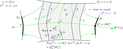
Figure 8: Dynamical thickening $(N,\theta)=(N^{s}_{x},\theta^{s}_{x})$ of ascending disk $W^{s}_{\varepsilon}(x)$

However, given the foliation in Theorem 5.1 of $N_{x}^{s}$ in terms of graphs, it is then a natural idea to turn this foliation into a dynamical foliation in the sense that each leaf will be endowed with its own flow. The natural candidate for these flows is our given flow $\varphi_{t}$ on the ascending disk $W^{s}_{\varepsilon}(x)=N^{s}_{x}\cap W^{s}(x)$ transported to any leaf via conjugation by the corresponding graph map; see Figures 8 and 9. This way the set $N_{x}^{s}$ turns into a disjoint union of copies of the dynamical system $(W^{s}_{\varepsilon}(x),\varphi)$. So one could call this procedure a dynamical thickening of the stable manifold; see [Web] for an application to a classical theorem.

Proof of Theorem 5.4.

Throughout we work in the local model provided by Definition 1.1. In particular, we will use these notation conventions in our construction of a strong deformation retraction $\theta$ of $N$ onto its part $D$ in the unstable manifold. As pointed out above on the stable manifold the forward flow $\{\phi_{t}\}_{t\in[0,\infty]}$ itself does the job. Indeed $\phi_{\infty}$ pushes the whole leaf $N(0)$, that is the ascending disk $W^{s}_{\varepsilon}$ by Theorem 5.1, into the origin – which lies in the unstable manifold. Since $\phi_{t}$ restricted to the origin is the identity, the origin is a strong deformation retract of $N(0)$. If the Morse index $k$ is zero, then $N=N(0)$ and we are done; similarly for $k=n$. Assume from now on $1\leq k\leq n-1$. The main idea is to use the graph maps ${\mathcal{G}}^{\infty}$ and $G^{T}_{\alpha}$ provided by Theorems 3.7 and 1.2, respectively, and their left inverse $\pi_{+}$ to extend the good retraction properties of $\phi_{t}$ on the ascending disk $N(0)$ to all the other leaves $N(\alpha^{T})$ provided by Theorem 5.1.

Definition 5.6 (Induced semi-flow – Dynamical thickening).

By Theorem 5.1 each $z\in N=N^{{\varepsilon},\tau}$ lies on a leaf $N(\alpha^{T})$ for some $T\geq\tau$ and some $\alpha$ in the ascending disk $S^{u}_{\varepsilon}$ and where $\alpha^{T}:=\phi_{-T}\alpha$. Then the continuous map $\theta:[0,\infty]\times N\to X$ defined by

$$\theta_{t}z:={\mathcal{G}}_{\alpha}^{T}\circ\pi_{+}\circ\phi_{t}\circ{\mathcal{G}}^{\infty}\circ\pi_{+}(z)={\mathcal{G}}_{\alpha}^{T}\circ\phi_{t}\circ\pi_{+}(z),$$ (68)

is called the induced semi-flow on $N$; see Figure 9. It is of class $C^{r}$ away from the stable manifold. Here (68) simplifies as ${\mathcal{G}}^{\infty}=(0,id)$ and $\pi_{+}|_{E^{+}}={{\mathchoice{\rm 1\mskip-4.0mul}{\rm 1\mskip-4.0mul}{\rm 1\mskip-4.5mul}{\rm 1\mskip-5.0mul}}}$.

Figure 9: Leaf preserving semi-flow $\theta_{t}$

Observe that while $\theta$ apriori only takes values in the image $F\supset N$ of the graph maps, it does preserve the leaves of $F$; see Corollary 5.3. Now continuity on $[0,\infty)\times N$ follows from continuity of the maps involved. Given $z\in N(\alpha^{T})$, set $z_{+}:=\pi_{+}z$. Since $z_{+}$ lies in the stable manifold by construction of our ”flat” coordinates, we obtain that $z_{+}(t):=\phi_{t}z_{+}\to 0$, as $t\to\infty$. So firstly the limit

$$\theta_{\infty}z:=\lim_{t\to\infty}\theta_{t}z={\mathcal{G}}^{T}_{\alpha}\lim_{t\to\infty}z_{+}(t)={\mathcal{G}}^{T}_{\alpha}(0)=\alpha^{T}$$

exists and lies in the unstable manifold indeed. Here we used continuity of ${\mathcal{G}}^{T}_{\alpha}$ and the final identity holds by Theorem 1.2. Secondly $\theta_{t}z\to\theta_{\infty}z$, as $t\to\infty$. This shows, firstly, that the map

$$\theta_{\infty}:N\to D,\qquad D=\phi_{-\tau}W^{u}_{\varepsilon}\cong\{0\}\cup\left([\tau,\infty)\times S^{u}_{\varepsilon}\right),$$ (69)

is a retraction and, secondly, that the map $\theta$ extends continuously to $[0,\infty]\times N$. The fact that the origin is a fixed point of $\pi_{+}$ and $\phi_{t}$ implies that

$$\theta_{t}\alpha^{T}={\mathcal{G}}^{T}_{\alpha}\circ\phi_{t}\circ\pi_{+}(0)={\mathcal{G}}^{T}_{\alpha}(0)=\alpha^{T}.$$

Hence $\theta_{t}|_{D}=id_{D}$, for every $t\in[0,\infty]$. It remains to show that $\theta_{t}$ actually preserves $N$. It suffices to show that $\theta_{t}$ preserves each leaf of the foliation

$$N=N(0)\cup\bigcup_{\begin{subarray}{c}T\geq\tau\\ \alpha\in S^{u}_{\varepsilon}\end{subarray}}N(\alpha^{T}).$$

In contrast to the infinite dimensional case [Web14b] a simple compactness argument will do. Note that any leaf, other than $N(0)=W^{s}_{\varepsilon}$, is of the form

$$N(\alpha^{T})={\mathcal{G}}^{T}_{\alpha}(B^{+})\cap\{f\leq c+{\varepsilon}\},\qquad{\partial}N(\alpha^{T})={\mathcal{G}}^{T}_{\alpha}(B^{+})\cap\{f=c+{\varepsilon}\},$$

whereas $N(0)={\mathcal{G}}^{\infty}(B^{+})\cap\{f\leq c+{\varepsilon}\}=W^{s}_{\varepsilon}$ and ${\partial}N(0)=S^{s}_{\varepsilon}$. Now since the boundary of $N(\alpha^{T})$ lies in a level set of $f$ and $\theta_{s}$ preserves the graph of ${\mathcal{G}}^{T}_{\alpha}$ we only need to show that there is a constant $-\mu<0$ such that

$$\left.\frac{d}{dt}\right|_{t=0}f(\theta_{t}z)\leq-\mu<0,\qquad\forall z\in{\partial}N(\alpha^{T}),\quad\forall\alpha^{T}\in D.$$ (70)

This means that the $\theta$ flow is inward pointing along the boundary of each leaf and then we are done. But (70) holds true for some constant, call it $-2\mu$, along the (compact) boundary $S^{s}_{\varepsilon}$ of the leaf $N(0)$, just because $\theta_{t}=\phi_{t}$ on $N(0)$ and $f$ strictly decreases along its downward gradient flow – unless there is a critical point which it isn’t on $S^{s}_{\varepsilon}$. Compactness of the leaf space $D$ and of the boundary of each leaf, together with continuity of the maps whose composition is $\frac{d}{dt}\theta_{t}$, then implies that (70) holds true for all nearby leaves. To restrict to nearby leaves just fix ${\varepsilon}>0$ sufficiently small and $\tau>1$ sufficiently large. ∎

Global foliation

To extend the foliation of the neighborhood $N_{x}^{s}$ of $x$ all along the stable manifold $W^{s}(x)$, that is in the backward time direction, according to Convention 1.5, that is without using the backward flow, is an interesting open problem – even more so in heat flow situations such as [Web14b].

References

- [AL93] R. P. Agarwal and V. Lakshmikantham. Uniqueness and nonuniqueness criteria for ordinary differential equations, volume 6 of Series in Real Analysis. World Scientific Publishing Co., Inc., River Edge, NJ, 1993.
- [BFK11] Dan Burghelea, Leonid Friedlander, and Thomas Kappeler. On the space of trajectories of a generic vector field. ArXiv e-prints, 01 2011.
- [BH04] Augustin Banyaga and David Hurtubise. Lectures on Morse homology, volume 29 of Kluwer Texts in the Mathematical Sciences. Kluwer Academic Publishers Group, Dordrecht, 2004.
- [Bot88] Raoul Bott. Morse theory indomitable. Inst. Hautes Études Sci. Publ. Math., 68:99–114, 1988.
- [CH82] Shui Nee Chow and Jack K. Hale. Methods of bifurcation theory, volume 251 of Grundlehren der Mathematischen Wissenschaften [Fundamental Principles of Mathematical Science]. Springer-Verlag, New York-Berlin, 1982.
- [Had01] J. Hadamard. Sur l’itération et les solutions asymptotiques des équations différentielles. Bull. Soc. Math. Fr., 29:224–228, 1901.
- [Hen81] Daniel Henry. Geometric theory of semilinear parabolic equations, volume 840 of Lecture Notes in Mathematics. Springer-Verlag, Berlin, 1981.
- [Hir76] Morris W. Hirsch. Differential topology. Springer-Verlag, New York-Heidelberg, 1976. Graduate Texts in Mathematics, No. 33.
- [Jos11] Jürgen Jost. Riemannian geometry and geometric analysis. Universitext. Springer, Heidelberg, sixth edition, 2011.
- [Law74] H. Blaine Lawson, Jr. Foliations. Bull. Amer. Math. Soc., 80:369–418, 1974.
- [Nic11] Liviu Nicolaescu. An invitation to Morse theory. Universitext. Springer, New York, second edition, 2011.
- [Pal67] Jacob Palis, Jr. On Morse-Smale diffeomorphisms. PhD thesis, UC Berkeley, 1967.
- [Pal69] Jacob Palis, Jr. On Morse-Smale dynamical systems. Topology, 8:385–404, 1969.
- [PdM82] Jacob Palis, Jr. and Welington de Melo. Geometric theory of dynamical systems. Springer-Verlag, New York, 1982. An introduction, Translated from the Portuguese by A. K. Manning.
- [Per28] O. Perron. Über Stabilität und asymptotisches Verhalten der Integrale von Differentialgleichungssystemen. Math. Z., 29:129–160, 1928.
- [Pes04] Yakov B. Pesin. Lectures on partial hyperbolicity and stable ergodicity. Zurich Lectures in Advanced Mathematics. European Mathematical Society (EMS), Zürich, 2004.
- [Qin11] Lizhen Qin. An application of topological equivalence to Morse theory. ArXiv e-prints, February 2011.
- [Sal90] Dietmar Salamon. Morse theory, the Conley index and Floer homology. Bull. London Math. Soc., 22(2):113–140, 1990.
- [Shu87] Michael Shub. Global stability of dynamical systems. Springer-Verlag, New York, 1987. With the collaboration of Albert Fathi and Rémi Langevin, Translated from the French by Joseph Christy.
- [SW06] Dietmar Salamon and Joa Weber. Floer homology and the heat flow. Geom. Funct. Anal., 16(5):1050–1138, 2006.
- [Tes12] Gerald Teschl. Ordinary differential equations and dynamical systems, volume 140 of Graduate Studies in Mathematics. Online edition, authorized by American Mathematical Society, Providence, RI, 2012.
- [Web] Joa Weber. Classical Morse theory revisited I – Backward -Lemma and homotopy type. arXiv 1410.0995, to appear in Topol. Methods Nonlinear Anal.
- [Web06] Joa Weber. The Morse-Witten complex via dynamical systems. Expo. Math., 24(2):127–159, 2006.
- [Web13] Joa Weber. Morse homology for the heat flow. Math. Z., 275(1-2):1–54, 2013.
- [Web14a] Joa Weber. A backward -lemma for the forward heat flow. Math. Ann., 359(3-4):929–967, 2014.
- [Web14b] Joa Weber. Stable foliations and semi-flow Morse homology. arXiv 1408.3842, submitted, 2014.
- [Zeh10] Eduard Zehnder. Lectures on dynamical systems. EMS Textbooks in Mathematics. European Mathematical Society (EMS), Zürich, 2010.