Evidence for Rapid Variability in the Optical Light Curve
of the Type Ia SN 2014J^,

We present results of high-cadence monitoring of the optical light curve of the nearby, Type Ia SN 2014J in M82 using the 2.3m Aristarchos telescope. $B$ and $V-$band photometry on days 15–18 after t${}_{max}(B)$, obtained with a cadence of 2 min per band, reveals evidence for rapid variability at the 0.02–0.05 mag level on timescales of 15–60 min on all four nights, taking the red noise estimation at face value. The decline slope was measured to be steeper in the $B-$band than in $V-$band, and to steadily decrease in both bands from 0.15 mag day^-1 (night 1) to 0.04 mag day^-1 (night 4) in $V$ and from 0.19 mag day^-1 (night 1) to 0.06 mag day^-1 (night 4) in $B$, corresponding to the onset of the secondary maximum. We propose that rapid variability could be due to one or a combination of the following scenarios: the clumpiness of the ejecta, their interaction with circumstellar material, the asymmetry of the explosion, or the mechanism causing the secondary maximum in the near-infrared light curve. We encourage the community to undertake high-cadence monitoring of future, nearby and bright supernovae to investigate the intraday behavior of their light curves.

1 Introduction

Nearby supernovae offer the opportunity to explore the short-timescale and low-amplitude variability properties of their light curves. Even though several nearby, bright supernovae (SNe) have been discovered recently (e.g. the Type Ia SN 2011fe and SN 2013aa, the Type IIP SN 2013ej; Nugent et al. 2011; Waagen 2013; Richmond 2014, respectively), no high-cadence variability search has been undertaken so far to explore variability on timescales of minutes or hours. Typical photometric monitoring of SNe consists of a single observation per night or every few nights in several filters, therefore, the intraday behavior of the light curves of SNe remains uncharted territory.

To rectify the situation, we performed high-cadence photometry of the nearby Type Ia supernova (SN Ia) SN 2014J (see e.g. Foley et al. 2014, and references therein), which was discovered in the galaxy M82 in January 2014 (Fossey et al. 2014). Reaching $V_{max}=10.61\pm 0.05$ mag (Foley et al. 2014), it was ideally suited for a variability search, which we conducted in February 2014 with the 2.3m Aristarchos telescope. Just before the submission of this work, Siverd et al. (2015) reported relatively high-cadence photometry of SN 2014J with the 4.2cm Kilodegree Extremely Little Telescope North (KELT-N), thereby placing a $4.5\%$ (3$\sigma$) upper limit on short timescale variations. This paper reports the results of our monitoring survey: the observations and data reduction are presented in Secion 2, the analysis in Section 3, the results in Section 4, and the discussion and conclusions in Section 5.

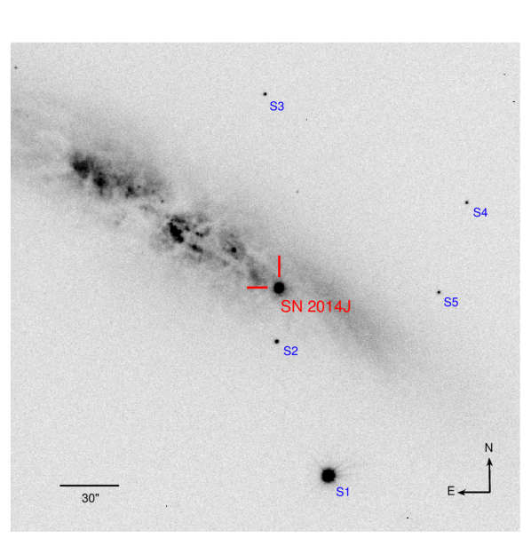
Figure 1: $V-$band image of SN 2014J in M82, obtained on 2014 February 16 with the Aristarchos telescope. The positions of the 5 comparison stars (S1–S5) used in the analysis are labelled.

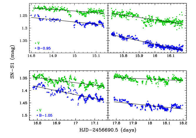
Figure 2: Calibrated $V-$band (circles) and $B-$band (triangles) differential light curves of SN 2014J, compared with Star 1, as a function of the time in days measured since t${}_{max}(B)=2456690.5$ (JD; Foley et al. 2014). Each panel corresponds to one night of observations. The $B-$band curves are offset by 0.95 mag in the upper panels and 1.05 mag in the lower panels for clarity. The black lines represent least-square fits to the photometry.

2 Observations and Data Reduction

SN 2014J was monitored for variability with the LN CCD camera on the 2.3m Aristarchos telescope for 4 consecutive nights: 2014 February 16–19 (nights 1–4 or N1–4), corresponding to days 14.8–18.2 after t${}_{max}(B)=2456690.5\pm 0.2$ (JD; Foley et al. 2014). The 1024$\times$1024 SITeAB back-illuminated CCD has pixels that are 24 $\mu$m in size, which map to $0.28\arcsec$ pixel^-1 on the focal plane, making each image $4.8\arcmin$ on the side. Figure 1 provides a finder chart, labelling the position of the SN and the comparison stars (S1–S5) used in the analysis below.

SN 2014J was observed for about 8 hrs per night to obtain differential photometry. Sequences of alternating $V-$band and $B-$band images were obtained with 5 sec and 20 sec exposure times, respectively, yielding 400–500 images per band each night and a cadence of 2 min per band. Small gaps in the data are mainly due to recentering performed in between typical sequences of 100 images, as the absence of guiding caused the target to drift during the sequences.

Initial reduction of the images was performed using standard routines in the IRAF ccdproc package (i.e. bias level subtraction, flat field division). The images were aligned with the IRAF imalign task, while the seeing was calculated using the IRAF task psfmeasure. The statistical mode values for the seeing in the $V-$band images each night were 1.2$\arcsec$​, 1.4$\arcsec$​, 1.2$\arcsec$​, 1.2$\arcsec$​, respectively, and 1.2$\arcsec$​, 1.6$\arcsec$​, 1.05$\arcsec$​, 1.25$\arcsec$​ in the $B-$band. Typical $\sigma$ values were 0.55$\arcsec$ for N2 and $0.2-0.3\arcsec$ for the other nights. Note, on N1/N3, the S/N of the maximum pixel value of S1 in $B$ (190/185) exceeded the mean S/N of the $B-$flat (176/172).

3 Analysis

Aperture photometry was extracted from the supernova and the 5 brightest comparison stars available in the field, using a 5 pixel or 1.4$\arcsec$ radius with the IRAF apphot package and a 5 pixel wide sky annulus 15 pixels from the source. Typical photometric errors are 1 mmag for the SN and S1, 0.01 mag for S2, and 0.01–0.02 mag for S3–S5.

The instrumental magnitudes for the SN and S1 were transformed to the standard system by computing zeropoint offsets and color terms, using $B$ and $V$ magnitudes for SN 2014J on N1 from Foley et al. (2014) and for S1 from the APASS Catalogue. The resulting transformation equations are:

$$V=v-1.320+0.056\cdot(B-V)$$ (1)

$$B=b-2.609+0.005\cdot(B-V)$$ (2)

where $b$ and $v$ are the instrumental magnitudes.

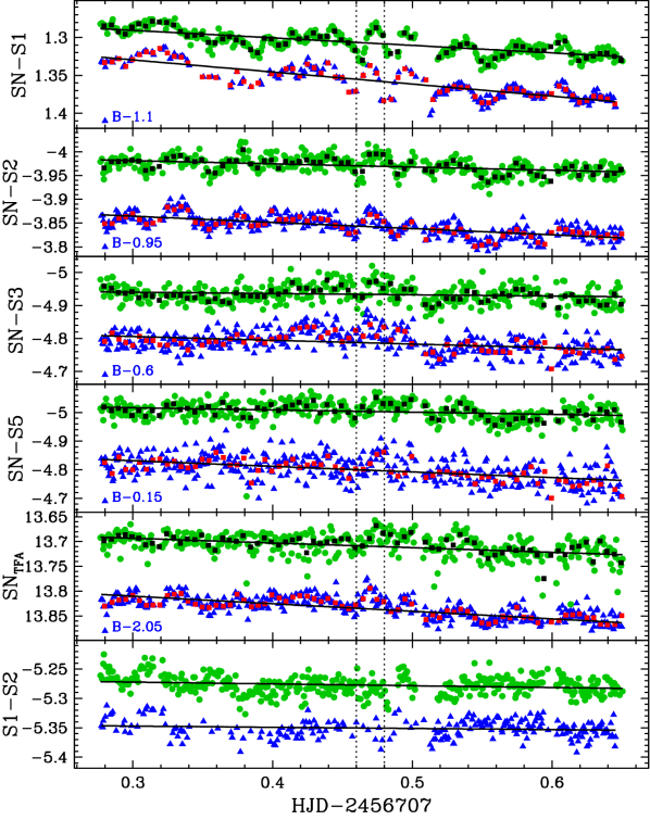
Figure 3: Instrumental $B-$band (blue triangles) and $V-$band (green circles) light curves of SN 2014J obtained on N3. The first four panels show the differential light curves of the SN with respect to S1–S3 and S5, respectively, followed by a panel showing the reconstructed light curves using the trend fitting algorithm (TFA) and the differential curve S1–S2. Solid lines correspond to least-square fits to the data, while black and red squares correspond to the binned $V$ and $B-$band light curve, respectively, using a bin size of 0.005 days. The $B-$band curves are offset for clarity by the amount indicated in each panel. Dotted lines indicate regions of significant variability.

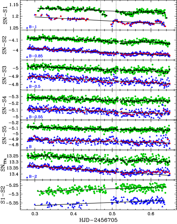
Figure 4: Same as Figure 3, but for N1. On this night all 5 comparison stars were available, therefore the first five panels show the differential light curves with respect to S1–S5, respectively, followed by a panel showing the reconstructed light curves using the trend fitting algorithm and the differential curve S1–S2.

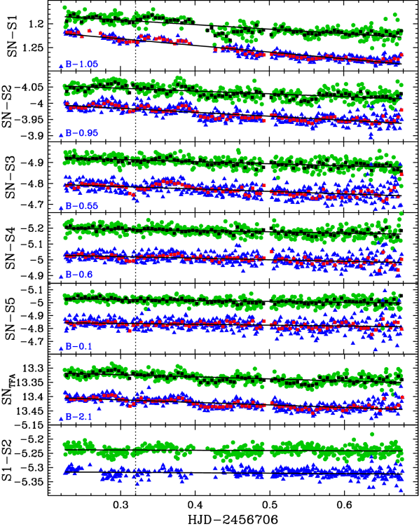
Figure 5: Same as Figure 4, but for N2.

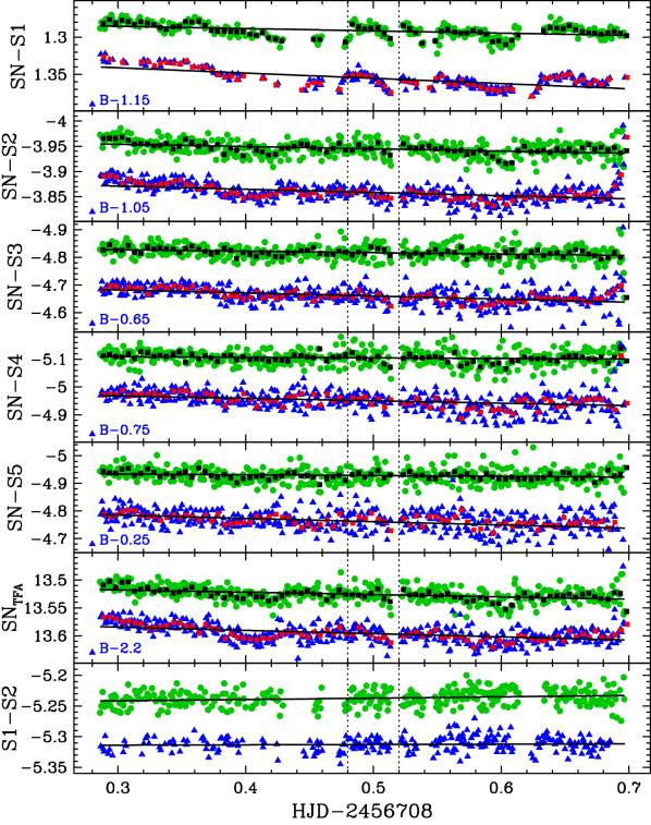
Figure 6: Same as Figure 4, but for N4.

Differential light curves were created by taking the difference between the instrumental magnitude of the supernova and each of the 5 comparison stars. S1 yields the smallest scatter, with an error in each point of 1.4 mmag. However, due to its brightness, it was saturated or exceeded the non-linearity limit of the CCD ($\sim 45000$ ADU) in the best seeing $B-$band images, creating gaps in the differential curves with respect to S1. Furthermore, the absence of guiding caused S1 to intercept a bad column, creating spikes in the light curves in both bands, which were selected visually and removed. Figure 2 presents the differential, calibrated, light curves with respect to S1, which show the expected decline of the SN and onset of the secondary maximum discussed below.

Figures 3–6 show the differential light curves with respect to all comparison stars available each night. We used a detrending algorithm to reconstruct the light curves, rule out intrinsic variability in S1 (as no variability information for S1 is available in the literature), and correct for systematic effects. We applied the Trend Filtering Algorithm (TFA; Kovács et al. 2005), as implemented in the VARTOOLS package (Hartman et al. 2008), using S2–S5 to reconstruct the light curves of the SN and S1. Due to the fact that S2–S5 are fainter, this method introduced noise at the level of $0.01-0.02$ mags to the light curves of the brighter stars, however, we found that the variability signal remains, although it is still affected by systematics. The two lower panels of Figures 3–6 present the detrended light curves and the differential curve S1–S2, respectively. The latter illustrates systematics present in the photometry, which are discussed in the next Section. Features that are present in all light curves (more clearly illustrated in the binned curves) and that correspond to a featureless S1–S2 curve provide evidence for rapid variability in the SN.

We next performed a test using artificial stars to assess the variability signal seen in the differential light curves. We inserted artificial stars to each of the $V-$band images taken on N3, which displays the largest variability, using the appropriate PSF derived for each image with the daophot package in IRAF. We inserted 3 stars at the magnitude of the SN along the disk of the galaxy at locations with both smoother and more complex galaxy background, 3 stars at the magnitude of S2 at the same distance from the galaxy disk, and 3 stars at the magnitude and distance of S1. We then performed aperture photometry, as described above, and constructed differential light curves. These were found to be dominated by Poisson noise and not to show any patterns resembling the varibility signal. In particular, the standard deviation ($\sigma$) of the points for the ’artificial’ SN in all 3 positions tested were $4.5-4.8$ mmag, while we found $\sigma=1.6$ mmag for SN$-$S1, $\sigma=0.0115$ mag for SN$-$S2 and $\sigma=0.012$ mag for S1$-$S2. The artificial star test thus provides additional support for the variability signal originating in the SN.

4 Results

The densely sampled differential light curves shown in Figures 2–6 provide a measure of the intranight decline rate of SN 2014J. Table 1 presents the decline rates measured each night in $V$ and $B$ based on least-square fits to the differential and detrended light curves shown in Figures 3–6. The error bars represent the root-mean-square (rms) error of the points to the fit. Note, the slopes inferred for SN–S1 are identical for the calibrated and instrumental light curves. All values are in agreement within errors, except for those derived using SN–S1 on N1, due to the larger gaps in the photometry on that night. Adopting the values derived from SN–S2, SN 2014J declines with a rate $\alpha$ of $0.15\pm 0.01$, $0.09\pm 0.01$, $0.07\pm 0.02$, $0.04\pm 0.01$ mag day^-1 in the $V-$band and $0.19\pm 0.01$, $0.12\pm 0.01$, $0.13\pm 0.02$, $0.06\pm 0.02$ mag day^-1 in the $B-$band, on N1–4, respectively. We therefore find the $B-$band to fade at a faster rate than the $V-$band, as expected, and the slope in each filter to vary from night to night. The decrease in the slope, observed in both bands, corresponds to the onset of the secondary maximum in the near-IR light curve (Kasen 2006; Jack et al. 2015), which is also seen in the light curves of SN 2014J presented by Foley et al. (2014), Amanullah et al. (2014), Marion et al. (2015), Kawabata et al. (2014), and Ashall et al. (2014).

Table 1: Decline rates $\alpha$ (mag day^-1) and values of $\sigma_{w}$, $\sigma_{r}$, $\sigma_{N}$ (mag) based on SN–S1 of the $V$ and $B-$band light curves of SN 2014J.

Night	Filter	$\alpha_{SN-S1}$	$\alpha_{SN-S2}$	$\alpha_{SN-S3}$	$\alpha_{SN-S4}$	$\alpha_{SN-S5}$	$\alpha_{SN_{TFA}}$	$\sigma_{w}$	$\sigma_{r}$	$\sigma_{N}$
1	$V$	$0.06\pm 0.01$	$0.15\pm 0.01$	$0.17\pm 0.02$	$0.15\pm 0.03$	$0.16\pm 0.02$	$0.14\pm 0.02$	0.0086	0.0045	0.0048
2	$V$	$0.09\pm 0.01$	$0.09\pm 0.01$	$0.10\pm 0.02$	$0.08\pm 0.03$	$0.07\pm 0.03$	$0.07\pm 0.01$	0.0107	0.0050	0.0053
3	$V$	$0.10\pm 0.01$	$0.07\pm 0.02$	$0.04\pm 0.03$	…	$0.08\pm 0.03$	$0.09\pm 0.04$	0.0177	0.0052	0.0061
4	$V$	$0.03\pm 0.01$	$0.04\pm 0.01$	$0.05\pm 0.02$	$0.02\pm 0.03$	$0.03\pm 0.02$	$0.04\pm 0.01$	0.0131	0.0046	0.0052
1	$B$	$0.09\pm 0.01$	$0.19\pm 0.01$	$0.24\pm 0.03$	$0.21\pm 0.03$	$0.17\pm 0.05$	$0.22\pm 0.05$	0.0104	0.0025	0.0031
2	$B$	$0.14\pm 0.01$	$0.12\pm 0.01$	$0.12\pm 0.03$	$0.10\pm 0.03$	$0.07\pm 0.04$	$0.09\pm 0.01$	0.0074	0.0033	0.0036
3	$B$	$0.16\pm 0.01$	$0.13\pm 0.02$	$0.11\pm 0.03$	…	$0.20\pm 0.04$	$0.15\pm 0.03$	0.0186	0.0036	0.0050
4	$B$	$0.07\pm 0.01$	$0.06\pm 0.02$	$0.11\pm 0.03$	$0.09\pm 0.04$	$0.12\pm 0.04$	$0.06\pm 0.01$	0.0128	0.0059	0.0063

More importantly, we report evidence for rapid variability in both the $V$ and $B-$band light curves of SN 2014J. We find that the level of variability varies from night to night and is best traced by the SN–S1 curve, due to the accuracy in the photometric measurements achieved for these bright stars. N3 and N4 exhibit the largest activity with sinusoidal-like variations of amplitude up to 0.05 mag, while variability on other nights is typically at the 0.02–0.03 mag level. A Fourier analysis of the SN-S1 curve did not yield a significant periodicity.

While the precision of our measurements, based on the 1$\sigma$ error bars resulting from the aperture photometry, is at the 1.4 mmag level for SN–S1 (and at the 0.6 mmag level for the binned curve), we must account for correlated sources of error (red noise) to quantify the significance of the variability detection. Sources of correlated error include the changing airmass, drifting of the stars across the CCD and other instrumental parameters. We follow the procedure outlined by Pont et al. (2006), which estimates the amount of correlated noise by calculating the dispersion $\sigma_{N}$ from the binned residuals (after subtracting a best fit model, in our case the decline rate) as a function of $N$ points and finds the values for the white ($\sigma_{w}$) and red ($\sigma_{r}$) noise that best fit the equation:

$$\sigma_{N}^{2}=\frac{\sigma_{w}^{2}}{N}+\sigma_{r}^{2}.$$ (3)

The estimated values of $\sigma_{w}$, $\sigma_{r}$ and $\sigma_{N}$ for each night and filter are shown in the last 3 columns of Table 1, using the SN–S1 data and $N=30$ ($\sim 1$ hour), which was selected to represent the longest timescale of the detected variability. Note, that the values computed with $N=10,\,20,\,40$ were very similar. If rapid variability is present, then the $\sigma_{N}$ values are overestimates, as all points of the light curves were used for the calculation. Given the derived $\sigma_{N}$ values (3–6 mmag), we find the 0.02-0.05 mag variations to be statistically significant. At face value, the 0.05 mag variation in N3 (at HJD=2456707.46–2456707.48) has a $8.2\sigma$ significance in $V$ and $10\sigma$ in $B$, and the 0.04 mag variation in N4 (at HJD=2456708.48$-$2456708.52) is a $7.7\sigma$ detection in $V$, and a $6.3\sigma$ detection in $B$. In N2, the 0.02 mag variation at HJD=2456706.32 is significant at the $3.8\sigma$ level in $V$ and $5.6\sigma$ in $B$, while in N1, the 0.03 mag variation (at HJD=2456705.47–2456705.51) is at the $6.2\sigma$ ($V$) and $9.7\sigma$ ($B$) level. The timescale of sinusoidal-like variations ranges from 15–60 min. On N3, the $B-$band is found to precede the $V-$band by $\sim 10$ min. The $B-V$ color gradually increases within each night, displaying an rms scatter of about 0.01 mag.

Table 2: Calibrated differential photometry of SN 2014J compared to S1 in the $V$ and $B-$bands.

HJD–2450000	Filter	SN–S1	$\sigma_{SN-S1}$
6705.30817	$V$	1.231	0.001
6705.31330	$V$	1.224	0.001
6705.31679	$V$	1.212	0.001
6705.31766	$V$	1.220	0.001
6705.31853	$V$	1.219	0.001

5 Discussion and Conclusions

The high-cadence, high-precision photometry obtained with the 2.3m Aristarchos telescope was crucial in providing evidence for rapid variability in the optical light curve of SN 2014J. A cadence of 30 min, such as that of the Kepler Mission, would not have been sufficient to detect the sinusoidal-like variations nor any variability pattern seen with the 2 min cadence of our observations. At face value, our photometric precision of 3–6 mmag (based on the estimation of red noise) or 2 mmag (based on artificial star tests on N3) for SN–S1 allowed for statistically significant detections of variability at the level of 0.02–0.05 mag on all nights, peaking on N3, implying that the phenomenon is common or perhaps even ubiquitous in SNe, unless it is produced by a mechanism related exclusively to the onset of the secondary maximum.

Theoretical models of SN light curves (e.g. Kasen et al. 2006; Sim et al. 2013; Fink et al. 2014) do not make predictions on such short time scales and therefore cannot be compared with the photometry presented here. We propose one or a combination of the following scenarios for the origin of the variability: (i) clumping of the ejecta, possibly caused by structures of intermediate mass elements in the outer layers (Hole et al. 2010), (ii) interaction of the ejecta with circumstellar material, inferred by Foley et al. (2014), (iii) asymmetry of the ejecta, as the explosion is not expected to be spherically symmetric (as inferred from spectropolarimetry, e.g. see review by Wang & Wheeler 2008), (iv) the onset of the secondary maximum, which corresponds to a sudden decrease in the flux mean opacity due to the transition from doubly to singly ionized iron group elements (see e.g. Pinto & Eastman 2000).

Using the photospheric velocity $\sim$2 weeks after maximum ($-10,600$ km s^-1; estimated from Fig. 15 of Foley et al. 2014), we estimate the SN to have a radius of 104 AU on day 17. The 0.02–0.05 mag variability corresponds to a fractional change of $\sim$2–5% in magnitude and flux, respectively, or a $\sim$1–2.5% fractional change in radius assuming constant luminosity and that the variation is due to a change of radius, i.e. 1–2.6 AU. The observed fluctuation, however, is an average variation of flux over the projected surface of the young remnant; the 1–2.6 AU radius change gives an estimate of the surface area fluctuating. Siverd et al. (2015) reported relatively high-cadence photometry of SN 2014J with the 4.2cm Kilodegree Extremely Little Telescope North (KELT-N), thereby placing a $4.5\%$ (3$\sigma$) upper limit on short timescale variations. The evidence for variability at the level of $2-5\%$ presented in this work is therefore consistent with the results of the measurement with KELT-N.

In conclusion, we strongly encourage the community to undertake high-cadence and high-precision monitoring campaigns of future, nearby and bright supernovae to confirm the presence of rapid variability, determine whether it occurs in both SNe Ia and II light curves, and differentiate between the scenarios for its origin. If variability is due to asphericity in the explosion, it will provide evidence for distinguishing the nature of SNe Ia progenitors (see Livio & Pringle 2011). Furthermore, light curve variability, if shown to be ubiquitous, is likely to contribute to the scatter in the mean magnitude of SN Ia calibrators, which remains one of the largest factors in the uncertainty of the Hubble constant (e.g. Riess et al. 2011). In any case, we expect rapid variability to provide a new window into the physics of supernovae.